Pollen clustering strategies using a newly developed single-particle fluorescence spectrometer

Abstract

Pollen is routinely monitored and forecasted with respect to public health and allergies, but monitoring networks generally utilize a manual process of collection, analysis, and modeling that leads to poor sampling density and high measurement cost. Here, we discuss application of a single-particle fluorescence sensor recently developed for the purpose of real-time detection and recognition of pollen and spores. The sensor operates by collecting fluorescence emission spectra from many individual pollen grains sampled onto a microscope slide for each of four excitation wavelengths (280, 350, 405, and 450 nm) associated with pollen fluorophores. The sensor also records major and minor diameters of each particle. Approximately 25–30 particles for each of eight commercially purchased pollen species were interrogated. Data were analyzed using four classification methods: hierarchical agglomerative and k-means clustering (unsupervised) and random forest and gradient boosting algorithms (supervised). The purpose of the manuscript is to show development of a computational strategy to analyze spectral input data of this kind in order to support further efforts to automate sensor data collection and analysis. Both unsupervised methods showed insufficient accuracy for separating pollen species (76% k-means, 9% HAC) whereas supervised methods performed similarly well (94–95%). The random forest algorithm was then utilized to further optimize operational parameters, based on its higher computational speed. Analyzing the relative importance of each optical source for sensor performance highlighted ways that may be useful to lower sensor cost with minimal reduction to analysis quality. The results provide a framework for the application of this and similar sensors to ambient pollen detection and classification.

Copyright © 2020 American Association for Aerosol Research

1. Introduction

Pollen grains are microgametophytes of seed-bearing plants that transfer genetic material for the purpose of reproduction and can be transported, e.g., by wind, water, insects, or flying animals (Conner et al. 1997). Airborne pollen, lofted into the air from species of plants that utilize wind for pollination (anemophilous), is the primary driver of allergic rhinitis that seasonally inflicts suffering on many millions of sensitized individuals around the world. It was recently estimated, for example, that costs related to pollen allergies had increased 73% from 2000 to 2005 alone, for a total economic impact of $11.2 billion (Songnuan 2013; Blaiss 2010). Further, the season of anemophilous pollen dispersal is growing both in temporal length and geographic area due to climate change (Richter et al. 2013), and so the global need to understand and mitigate influence from airborne pollen allergies continues to grow.

Many countries or continental regions operate national networks of pollen monitors for the purpose of public health information. In continental Europe, for example, a well-developed network of sites (>525) collect data about relative levels of key allergenic pollen and fungal spore species on a daily basis, whereas in the United States a smaller network of ∼150 stations is operated (Buters et al. 2018). An interactive pollen measurement global map assembled by the Center for Allergies and Environment in Munich, Germany shows high density of pollen measurement in most of Europe, the Eastern United States, and Japan, additional points around China and Australia, and then at best sparsely scattered measurements across the rest of the world (Buters et al. 2018). In almost all cases pollen collection is performed by impacting airborne particulate matter onto sticky collection surfaces (Frenz 1999), and analysis is performed manually by trained palynologists who analyze collected material by visual microscopy (Erdtman 1952). This process is costly due to the requirement of using technicians trained in the specialized biological identification process, provides data at relatively low time resolution (min. 2+ hr), and leads to poor spatial resolution of sampling sites. For example, only ca. 20 monitoring sites are operated in the vast geographic region of the western United States, and many states have no sites at all (American Academy of Allergy Asthma & Immunology 2019). Pollen counts at locations between measurement sites are interpolated, and thus the quality of prediction at the local level varies significantly. Local and regional topological effects also influence pollen measurement and prediction accuracy (Tseng and Kawashima 2019). Data from pollen monitoring stations are combined with meteorological conditions as input parameters for predictive models. The result is to forecast, e.g., the beginning date of pollination season and the relative concentration of key allergenic pollen classes as a function of geography (Pauling et al. 2012; Stach et al. 2008; Galán et al. 2001). These forecasts are frequently then transmitted to the public via news organizations and smartphone applications.

As a result of the challenges of relying on manual identification processes, significant effort has gone into finding automated solutions to replace or supplement existing detection strategies (e.g., Huffman et al. 2019; Wu et al. 2018; Kawashima et al. 2017; Tello-Mijares and Flores 2016; Oteros et al. 2015; Kiselev, Bonacina, and Wolf 2013; Dell’Anna and 2010; Allen et al. 2008; Ranzato et al. 2007; Chen et al. 2006). Efforts to automate pollen analysis continue to face a variety of technical challenges (Šantl-Temkiv et al. 2019), and so at present only a few areas of the world have experimented with deploying prototypes of automated techniques. The allergenic pollen burden of many regions of Japan is heavily dominated by a single pollen species (Japanese cedar), and so a single-particle light-scattering instrument (KH-3000; Yamatronics, Japan) was developed largely to quantify this pollen type (Kawashima et al. 2007, 2017) in networks around the country (Miki et al. 2019; Kawashima et al. 2017). The KP-1000 (Kowa Company, Ltd.; Tokyo, Japan) also focuses on the selective detection of Japanese cedar, but applies principles of flow cytometry to measure the ratio of blue to red fluorescence and scattering intensity (Mitsumoto et al. 2010). The BAA500 (Hund-Wetzlar; Wetzlar, Germany) was developed to mimic the operational process of collection and microscopy analysis, and is being used in small numbers in a pollen monitoring network in southern Germany (Oteros et al. 2015). Many examples of ultra-violet laser-induced fluorescence (UV-LIF) instruments have been utilized to selectively detect biological fluorophores in atmospheric particulate matter and have been applied not only for pollen detection, but for rapid detection and classification of a wider range of biological aerosol types including bacteria and fungal spores (Huffman et al. 2019; Fennelly et al. 2017; Pöhlker, Huffman, and Pöschl 2012, Pöhlker et al. 2013; Després et al. 2012; Pan et al. 2011; Hill, Mayo, and Chang 2009). The Wideband Integrated Bioaerosol Sensor (WIBS, Droplet Measurement Technologies; Longmont, Colorado) uses two excitation sources (280 nm and 370 nm) to selectively target biofluorophores, capturing fluorescence signals with coarsely binned resolution of two channels per emission spectrum (Savage et al. 2017; Hernandez et al. 2016; Gabey et al. 2010; Kaye et al. 2005). The WIBS has been applied for pollen detection, but with only limited success (Calvo et al. 2018; Ruske et al. 2018; Savage and Huffman 2018; Savage et al. 2017; Perring et al. 2015; O’Connor et al. 2014; Kiselev, Bonacina, and Wolf 2013; Healy et al. 2012; Healy et al. 2014). The Rapid-E (Plair SA; Geneva, Switzerland) acquires fluorescence spectra in 32 channels after excitation by a 400 nm laser and also records fluorescence lifetime and time-resolved light scattering signal in order to more finely differentiate between pollen species (Kiselev, Bonacina, and Wolf 2011, 2013). The Rapid-E has been applied to ambient pollen monitoring in several studies, and shows the ability to discriminate between certain groups of pollen types with ∼90% accuracy (Šaulienė et al. 2019; Crouzy et al. 2016). The Poleno instrument (Swisens AG; Horw, Switzerland) acquires fluorescence spectra as well as time-resolved scattering and holographic images. The instrument was recently shown capable of identifying ten pollen species in ambient air when utilized with convolutional neural networks (Sauvageat et al. 2019). While these few examples of instrumentation able to identify or differentiate broad classes of pollen are under investigation for application for monitoring networks, their purchase cost is high, e.g., fifty to hundreds of thousands of dollars per unit. As a result, the need exists to dramatically reduce the purchase cost of pollen sensors capable of recognizing key pollen species in real-time.

A variety of multivariate analysis algorithms have been applied to the differentiation of spectral data from UV-LIF and other bioaerosol sensors (Huang et al. 2011; Pinnick et al. 2004). Algorithms can be divided into supervised or unsupervised classification techniques, where supervised techniques require prior input of data to train clusters, whereas this is not required for unsupervised techniques (Mohri, Rostamizadeh, and Talwalkar 2018). Unsupervised methods can thus be attractive to analyze particles from ambient observations, because no prior input is needed and so properties of test data do not bias results. For example, k-means clustering (unsupervised) was first applied to atmospheric aerosol data at least as early as 2004 (Erdmann et al. 2005), and has also been applied more recently, including with respect to particulate matter investigated using aerosol time-of-flight mass spectrometry and sun photometry (Elangasinghe et al. 2014; Rebotier and Prather 2007; Knobelspiesse et al. 2004). Unsupervised hierarchical agglomerative clustering (HAC) has also been frequently applied to study UV-LIF bioaerosol data, e.g., applied to WIBS data (Forde et al. 2019; Savage and Huffman 2018; Crawford et al. 2015; Robinson et al. 2013), and to fluorescence spectra from instrumentation that acquires LIF spectra at higher resolution than the WIBS (Könemann et al. 2019; Zhu, Liu, and Wu 2015; Pan et al. 2003).

Supervised clustering techniques can be effective analysis tools, especially when data is labeled (i.e. the identity of an observation is known). Ensemble methods, a subset of supervised methods that combine multiple learning algorithms in succession, can generally provide higher classification accuracy than unsupervised methods (Rokach 2010). The random forest (RF) classification technique is an ensemble algorithm that has previously been shown effective in differentiating bioaerosols (Ruske et al. 2017). The RF technique utilizes many parallel decision trees, each of which performs classifications via a series of decision nodes, by random bootstrap sampling of input variables. Tree decisions are then averaged to match an observation to the best matching input cluster. The RF technique has been shown to produce results with intermediate-quality separation accuracy (>74% for laboratory generated aerosols), but without requiring high computing power (Ruske et al. 2017). Gradient boosting (GB), another ensemble method, similarly creates small decision trees, with the exception that all variables are initially weighted equally and examined (Friedman 2001). The developed trees are then analyzed for variables that lead to misclassifications, and variables are re-weighted in order to circumvent misclassifications (Friedman 2001).

Within the last few years, the development of small and relatively inexpensive instrumentation for pollen detection has become more popular (Huffman et al. 2019). In most of these cases, the physical principles of detection are based on light-scattering, pattern recognition, or holography, using advanced analysis computing to differentiate pollen types using field-portable instrumentation. One such prototype sensor generates diffraction holograms associated with individual particles, and deep learning techniques are then utilized to process and subsequently classify, or label, the measured particles from the hologram (Lee, Yaglidere, and Ozcan 2011). The sensor was shown to successfully separate a laboratory-generated mixture that included three species of pollen (Bermuda grass, oak, and ragweed), two fungal spore types, and common dust, with a classification accuracy of 94% (Wu et al. 2018). Another recently available commercial sensor is the Pollen Sense™ (Pollen Sense, Salt Lake City, Utah), which is a portable and relatively low cost (∼$6,000) sensor that utilizes a combination of visual microscopy and image analysis techniques to identify pollen types as well as other large particles (http://pollensense.com).

Building upon a long history of pollen research using UV-LIF techniques and adding the goal of small sensor deployment, we previously developed an inexpensive sensor with intended application toward autonomous collection and identification of airborne pollen and fungal spores (Swanson and Huffman 2018; Huffman, Swanson, and Huffman 2016; Huffman and Huffman 2019). The level of differentiation required between pollen types will depend on specific applications or needs (Šantl-Temkiv et al. 2019). In some cases separation and identification of many individual species may be desirable, whereas in other cases it may be necessary to quantify only a few allergenic species out of a bulk of pollen types (analogous to the detection of Japanese cedar pollen, i.e. Kawashima et al. 2007, 2017). Previously published work (i.e. Swanson and Huffman 2018) utilized only a small fraction of the acquired spectral data for analysis and so particle differentiation capabilities were limited. To more fully investigate the capabilities of the sensor with respect to pollen classification, in this study we first present improvements made to the sensor and to the image-processing procedure in order to utilize higher quality fluorescence spectra. Using this updated process, data was collected from 25–30 particles for each of eight different pollen species. At present operation, spectral data are collected manually and relatively slowly from small numbers of pollen particles, though parallel work is on-going to improve analysis throughput for increased speed and particle detection statistics. Two unsupervised clustering techniques (k-means and HAC) and two supervised classification techniques (GB and RF) were compared with respect to their ability to differentiate individual pollen grains between different species. Both unsupervised techniques showed clustering results insufficient for further application, and so only RF and GB algorithms were further refined to optimize pollen separation. The primary purpose of this article is to compare and discuss several commonly used computational strategies applied to analysis of single particle spectral data from a small test set of pollen types in order to support development of the sensor and related instruments. Further work is intended to apply results of the computational strategy to larger sets of pollen data. The clustering applications discussed here utilizing spectral data from this instrument show how optimizing the clustering process can improve particle differentiation with respect to the specific sensor and also have broad application to a growing number of techniques that utilize pollen data collected from other UV-LIF instruments.

2. Instrument and classification methods

2.1. Single-Particle fluorescence sensor

2.1.1. Sensor operation

Spectral data was collected here using the sensor and methods previously described (Swanson and Huffman 2018; Huffman, Swanson, and Huffman 2016), however a summary of the sensor operation is provided here for clarity. See also Figure 1 in the online supplementary information (SI) for a schematic diagram of the instrument. Particles are collected manually on a standard glass microscope slide prior to measurement and placed onto the microscope stage. Four excitation sources are used in sequence to illuminate particles: 280 nm LED (0.33 mW, ball lens; QPhotonics, Ann Arbor, Michigan), 350 nm LED (5.0 mW, flat window and focusing lens tube; QPhotonics), 405 nm laser diode (50 mW; Power Technology, Little Rock, Arkansas), and 450 nm laser diode (4.5 mW; Thorlabs, Newton, New Jersey). A 632.8 nm Helium-Neon laser (Meredith Sensors HNS-LL-1; Peoria, Arizona) is utilized for a two-point wavelength calibration of each image. Light reflected or emitted from each particle is collected and magnified through two microscope lenses, passed through an optical filter and diffraction grating (300 grooves mm⁻¹; Thor Labs), and collected by a CCD camera (Lumenera 2-1 R; Ottawa, Ontario Canada). In this way, fluorescence spectra from pollen grains or other fluorescent particles appear as swaths of light originating from each individual particle. Each light source is directed at the same spot on the microscope slide to simultaneously illuminate many particles present in a single image viewing area of approximately 1.0 x 1.0 mm. Figure S2 shows an example image where many swaths (fluorescence spectra) can be seen simultaneously illuminated. The process allows for collection of particle size (major axis, minor axis, and aspect ratio) and emission spectra (400–700 nm) at each wavelength of excitation, all for each individual particle. A total of five images are collected for each particle. Four images correspond to the four excitation wavelengths used to extract emission spectra, and a final image is used for wavelength calibration. By measuring the distance (in camera pixels) between the dispersion between the 403.5 nm (blue) and 632.8 nm (red) laser lines, the emission spectra can be calibrated from pixels to wavelength (nm).

Figure 1. Particle sizing methods. (a) Example of fluorescence swath image used in previous method to measure particle size. Vertical red lines represent region in which light intensity was averaged in horizontal dimension. (b) Transect of light intensity from (a) and Gaussian fit. FWHM represents particle size measurement (26.5 µm). (c) Blue ellipse shows scattering image of an individual particle under red laser illumination. Particle size from (c): major and minor axes (38 and 36 µm) and Y and X dimensions (35 and 34 µm). Full images for (a) and (c) shown in Figure S3.

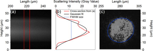
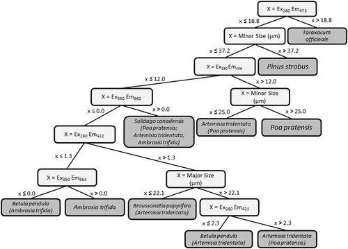
Figure 2. Single conditional tree (#243) from a 500-tree RF classification of the entire pollen data set. Tree shows the decisions involved in classification of all 8 species. Highest impact variables are listed in light gray, output nodes in dark gray. Main pollen species node stated in output node, with any misclassified species listed in parenthesis.

2.1.2. Particle sizing procedure

The particle sizing method as previously described utilized the width of the fluorescence swath measured by the sensor (Figures 1a,b and S3) as a proxy for particle diameter (Swanson and Huffman 2018). The profile across the swath of light is extracted (red curve, Figure 1b), and a Gaussian distribution is fit to the profile (black curve, Figure 1b). The full width at half the maximum peak height (FWHM) is then taken as particle size. This method provides accurate sizing for spherical, homogeneous particles such as polystyrene spheres used for sizing calibration, as was shown previously (Swanson and Huffman 2018). The FWHM method can lead to sizing errors for particles with non-spherical morphology or inhomogeneous mixing of fluorophores, however. The swath of light diffraction through the grating is approximately the same height in the vertical dimension as the particle, but only with respect to the orientation of the particle on the stage. Oblong particles (i.e. aspect ratios higher than 1:1) can have any orientation, and so monodisperse particle of oblong shape exhibit a wide distribution of particle sizes. Additionally, particles that exhibit inhomogeneous composition or that contain areas with weak fluorescence (i.e. pollen grains with air pockets or lower fluorophore density) can show variations in fluorescence profile across the CCD image (e.g., bimodal distribution in Figure 1b). Thus, the profile quality can vary also as a function of material composition, and calculated size will not be accurate.

To reduce sizing uncertainties from the effects mentioned above, an updated technique was developed to directly measure and record particle size and shape using the image of the particle. Raw calibration images are collected using simultaneous illumination by red and blue lasers, with the grating in place to disperse red and blue scattering points from one another. Particles are detected in calibration images automatically using Igor Pro analysis software (Wavemetrics; Lake Oswego, Oregon), searching the image at locations matching the diffraction angle from the red laser. A numerical threshold (T1), generally between 25 and 100 intensity units per pixel, is applied to the images to convert light intensity values to binary. The T1 value is assessed for 1–2 particles per experiment by visually comparing with the original calibration image to ensure the size of the binary mask qualitatively matches the tested particle. The number of counted pixels within each particle ellipse are counted, and particles below a chosen threshold (T2) corresponding to approximately 10 μm in diameter are filtered out to limit detection of small particles and scattering artifacts. For each detected particle, the major and minor diameters are recorded using properties of the measured ellipses (Figure 1c).

2.1.3. Spectral calibration

Spectral calibration was performed using methods reported previously (Swanson and Huffman 2018), except that here fluorescence intensity was normalized by the y-dimension of particle size to correct for differences. Previous particle size measurements had been performed by measuring the width of the fluorescent swath, so for comparison with that method the magnitude of the vertical component of each particle (ellipse after T1 and T2 applied) was extracted and used for normalization. For data presented here, excitation exposure time was manually modified as a function of particle size, composition, and excitation source. Larger particles, on average, were subjected to shorter exposure times due the corresponding increase in emission intensity with size. Each emission spectrum was normalized by the exposure time (in milliseconds) associated with the emission image. Light-power density from each source was treated as previously described by normalizing observed emission intensity by the estimated light power density at the location of excitation (Swanson and Huffman 2018).

Spectra utilized for clustering trials discussed in Sections 3.3 and 3.4 were filtered to remove noise in the tails of the spectra when intensity values were less than approximately 0.1 arbitrary units. This noise filtration restricts the emission spectral range to 440–620 nm following 350 nm excitation, 440–650 nm following 405 nm excitation, and 450–670 nm following 450 nm excitation. Emission spectra following 280 nm excitation were not affected (range 400–560 nm). Further detail regarding the noise filtering process is discussed in SI section S1.

2.2. Pollen samples

Eight pollen species were chosen to represent a wide variation of plant species for investigation. Pollen were purchased from Allergon AB (Ängelholm, Sweden): Poa pratensis (Kentucky bluegrass; 011608102); from Sigma-Aldrich (Munich, Germany): Artemisia tridentata (big sagebrush; P9520); from Polysciences (Warrington, PA, USA): Broussonetia papyrifera (article mulberry; 07670); and from Bonapol (České Budějovice, Czech Republic): Ambrosia trifida (giant ragweed; 294-01-1-10), Betula pendula (silver birch; 134-04-1-13), Pinus strobus (eastern white pine; 225-02-1-15), Solidago Canadensis (Canadian goldenrod; 262-05-1-12) and Taraxacum officinale (common dandelion; 241-01-1-07). All pollen samples were deposited onto a pre-cleaned microscope slide by shaking a small amount of pollen out of a plastic bag or by impacting using an aerosol collector and pump.

2.3. Clustering methods

Classification algorithms group observations (particle characteristics that represent a cluster) based on the variables associated with each observation (Percy and Everitt 2006). Four techniques were chosen for study here to compare both accuracy and efficiency of analysis with respect to data collected from the sensor: k-means, HAC, random forest, and gradient boosting.

An individual particle is represented in each algorithm as a series of 1,063 variables: major and minor particle size axes, size aspect ratio, and emission spectra for each excitation wavelength. Emission spectra were input with a range of 400–700 nm at 1 nm resolution, with exception of the 280 nm excitation where a range of 400–560 nm was used to avoid 2^nd order scattering effects. Emission spectra for the initial comparisons of k-means and HAC were scaled by the z-score method (Crawford et al. 2015). HAC, k-means, and RF all required ∼3 s to compute a solution for 204 particles with 1,067 variables for each particle, whereas GB required 57 s.

Directly comparing the results of the unsupervised methods to the supervised methods can be misleading, because of the manner in which the general classes of algorithms operate. The two unsupervised methods produce results channeled into the number of clusters determined by the human operator, but without utilizing any supervisory signal (i.e. average spectral parameters that describe an individual pollen species). In contrast, the two supervised methods build a training model by fitting individual particles into clusters that most closely match the supervisory signal associated with a given pollen species. As a result, supervised techniques will almost always produce clusters more accurately separated than by unsupervised techniques, and directly comparing accuracy of results across the two general classes has little meaning. Here we investigated the capability of two unsupervised techniques to separate individual pollen grains as a means of evaluating whether these could be candidates for future analysis. Unsupervised techniques provide weaker guides to particle differentiation, but allow particles of unknown or unique origin to be classified into unique clusters (Mohri, Rostamizadeh, and Talwalkar 2018). In contrast, supervised techniques provide higher accuracy as long as input data (supervisory signals) accurately represent the particle types in a given sampling experiment. In cases where unique particles are observed, however, these will be forced into a cluster whose supervisory signal is closest, even if incorrect. Thus, classification accuracy using supervised signals is only as good as the breadth and quality of the input data supplied (e.g., Huffman et al. 2019; Ruske et al. 2018).

Supervised techniques can also suffer from overfitting (also called overtraining), which means that the statistical model developed by the algorithm too narrowly defines the properties of a given cluster (Dietterich 1995). This can happen when the model defines a particle as a member of a given class only if its properties exactly match one of the existing members, without, e.g., averaging or interpolating the properties. This results in exclusion of any particles from a test set unless they are identical to particles in the train set, and so the model loses effectiveness.

2.3.1. k-means clustering

The k-means clustering algorithm utilizes an iterative process of randomly choosing data observations (k) as cluster centroids (Hartigan and Wong 2006). The observations are then partitioned based on the cluster centroid into a Voronoi partition, and new centroids are calculated based on these groupings. The algorithm continues this process until it converges to a local optimum and the centroid values no longer change. The k-means clustering algorithm was previously explored briefly using data from the sensor (Swanson and Huffman 2018) using 4 pollen species and reduced input data (height and position of emission spectral peak maximum). This process showed the ability to separate broadly between pollen species with wide taxonomic differences as a proof-of-concept, however the use of simplified data does not facilitate differentiation of pollen based on subtle features in the emission spectra.

Cluster analysis using the k-means algorithm was performed here as a semi-unsupervised process, in contrast to the method applied previously (Swanson and Huffman 2018), where the technique was applied in an unsupervised manner. This means the cluster centroids were not pre-defined here, and only cluster number (k = 8) was prescribed to the algorithm. The k-means algorithm was also previously shown to produce relatively high misclassification of ambient bioparticles detected by a WIBS due to the limited nature of the unsupervised method used within this algorithm (Ruske et al. 2017), but exhibited relatively high accuracy using data obtained from the sensor discussed here (Swanson and Huffman 2018). When allowed to iterate until optimal clusters are created, the k-means algorithm produces clusters with similar group size (Percy and Everitt 2006). This does not present problems for the data presented here, but may introduce errors when unknown numbers of pollen species are involved, e.g., in ambient samples (Geburek et al. 2012). The k-means clustering algorithm is available as a built-in statistical package for R (RStudio Inc., Boston, MA).

2.3.2. Hierarchical agglomerative clustering

The hierarchical agglomerative clustering algorithm initially uses the number of clusters matched to the number of measured particles, and groups data by Euclidian similarity until a single cluster remains. The user is then required to choose the appropriate number of clusters based either on a priori knowledge of the number of particle types or by using HAC-specific tools such as the Calinski-Harabasz Index that examines inter- and intra-class distance ratios (Liu et al. 2010). Allowing the algorithm to determine the optimal cluster number can be powerful, because previously unknown properties can be revealed (Robinson et al. 2013). HAC analysis has been applied to single-particle LIF data with relative success (Pan et al. 2012; Pinnick et al. 2004). Labeled and unlabeled data can both be examined by these unsupervised techniques by removing data labels to treat all data as unknown. The HAC output can be visualized using a dendrogram, which shows distances between observations in a representative tree diagram and which will report particle grouping from the top down. The dendrogram can be chopped at the desired number of clusters (e.g., n = 8) for the final classification solution. Several linkage methods exist for the HAC algorithm, including single, average, weighted, complete, and Ward’s (Crawford et al. 2015). The ward.D2 method was used in this study, similar to a previous study in which pre-labeled data was clustered utilizing HAC (Savage and Huffman 2018). HAC is available in the fastcluster package, an open source tool for R.

2.3.3. Random Forest algorithm

Random forest classification is a supervised ensemble algorithm that utilizes decision trees to group observations based on bootstrap sampling of the data (Breiman 2001). Decision trees classify observations by making individual node decisions to separate observations but can suffer overfitting by developing a model that memorizes the data. In this case, an individual decision tree may produce accurate results for the training data, but less accurate results for the subsequent data being tested (Dietterich 1995). RF classification algorithms use many conditional decision trees that are developed in parallel, utilizing random variations of the variable inputs (Hothorn et al. 2004; Breiman 2001). The RF method allows for development of both representative and overfitted trees, though to a much lesser degree of overfitting compared to GB. Using a large number of trees for analysis allows many of the trees to be developed simultaneously, the majority of which should represent the data accurately. Changes in decision tree population (forest) can affect classifications and utilizing the optimal number of variables compared at each decision node implies inherent tradeoffs between developing trees that examine the variables properly and that memorize the data.

Random forests have been employed for bioaerosol analysis and showed similar performance to other supervised techniques such as GB and neural networks, but with lower computational burden (Ruske et al. 2017). Random forests have also been used, e.g., for genetic mapping, which requires use of a large number of variables from the sample data (Bureau et al. 2003). RF classification was performed here using the open-source ‘party’ package within R. The cforest tool (conditional RF algorithm available in the ‘party’ package) uses unbiased processes in the decision making. Unlike the base implementation of random forest within R, cforest trees are initially developed, then conditional inference trees are fitted to the originally developed bootstrap trees, and the averaged observation weights from the trees are reported rather than simple average values from the bootstrap trees (Hothorn et al. 2015). These two differences result in predictive models that are more accurate, but more computationally expensive. For initial testing, the number of trees used here was held at 500, and the number of variables was left at the package default of five.

An individual tree for the RF model can be plotted in order to visualize the decision-making process within the algorithm. This was shown for the entire data set in Figure 2 as an example, in which the 243^rd tree is represented from a 500-tree forest. This tree classified the 204 particles through separations at nine distinct decision nodes. For the first decision node, the tree displays the most important variable of 50 chosen randomly from 1063 input variables: emission intensity at 473 nm following excitation at 280 nm. Particles with emission intensity >18.8 at this wavelength were classified into cluster 8, ascribed as T. officinale. This delineation was effective, because no other species contained particles with emission intensity > 18.8. For example, see relative differences in pollen species with respect to emission spectra following excitation at 280 nm (Section 3.1). Each subsequent branch of the tree shown in Figure 2 separates observations based on other variables until final clusters are formed.

The RF algorithm, as initially operated, provided high classification accuracy, however improvements can be made by manipulating input parameters that affect development of the model. Increasing in the number of trees from 1 to 2000 provides higher accuracy, but the relative improvement diminishes as the model converges to optimal accuracy at ∼500 trees (Figure S4). Variable number examined per node can also be changed from a default value (‘mtry’ = 5). Increasing variables examined per node can ultimately allow development of identical (overfitted) trees, thus limiting the advantage a RF has over other techniques. To avoid this issue, mtry was left at 5. A 500-tree forest was used for the initial testing, and a forest of 1000 trees was used for Sections 3.3 and following.

2.3.4. Gradient boosting algorithm

Gradient boosting is a supervised ensemble classifier algorithm that uses smaller, weaker decision trees than the RF technique (Friedman 2001). The term “weaker trees” implies that they are developed with a single decision node to separate a fraction of the data per each weak tree. These weaker trees are used in an iterative fashion, as opposed to being developed simultaneously as in RF, where the overall model is re-trained to reduce mean squared error over the series of weak decision trees. Instead of randomly selecting variables, all variables are weighted equally and each iteration re-weights variables based on an exponential loss function. Variables are re-weighted based on misclassification performance in each decision tree, and the algorithm iterates repeatedly over a given number of trees. The algorithm process allows for a number of sequential decision trees to be made into a model that can accurately separate sections of data for each individual decision tree.

GB algorithms have shown relatively high accuracy with respect to sorting bioaerosol classes, though at higher computational cost than the RF algorithm (Ruske et al. 2017). Overfitting the data can occur frequently, so cross-validation can be performed automatically within the model through data sub-sampling (Friedman 2001). Sub-sampling allows the data to be split into k number of groups, which are then used to take k-1 groups to develop a training mode used to test on the remaining group (James et al. 2013). The test-set error from sub-sampling is used to determine optimal tree iteration, which is the ideal position in the model to predict new data. GB was performed using a multinomial distribution; cross-validation folds of 10, and 500 trees, and is available from the ‘gbm’ package for R.

When improving the classification accuracy for GB, the risk of overfitting is present, though this can be mitigated with tools from the gbm package. Cross-validation can be used to develop an exponential loss curve that analyzes the difference in error associated with the training and testing sets (Figure S5). Other gbm parameters were investigated, including shrinkage, interaction.depth, and n.minobsinnode. The effects each of these played on the data set were minimal, and default parameters led to accurate predictions. A model with 10-fold cross-validation was used in all circumstances, and the ideal iteration was used to predict data for Section 3.3.

2.4. Performance and validation of algorithms

2.4.1. Particle misclassifications and total error

Classification results are shown in confusion matrices (e.g., see Section 3.2), which visually describe the accuracy of classifications with respect to input category and output cluster. Particle misclassifications are described in terms of precision (false-positive) and recall (false-negative). Precision describes the ratio of particles incorrectly classified to a cluster (vertical misclassifications), to the number of particles correctly classified to the cluster. Recall describes the ratio of particles incorrectly classified from a cluster (horizontal misclassifications), to the number of correctly classified particles. A value of 0.0 for precision or recall variables describes misclassification, whereas a value of 1.0 describes correct classification. The precision and recall variables are used to calculate the mean F value for a species, e.g., averaged over a calculated cluster using the following equation (Buckland and Gey 1994): $$F\mathrm{}=\mathrm{}\frac{\left(2\mathrm{}x\mathrm{}\mathit{False}\mathrm{}\mathit{Positive}\mathrm{}x\mathrm{}\mathit{False}\mathrm{}\mathit{Negative}\right)}{(\mathit{False}\mathrm{}\mathit{Positive}\mathrm{}+\mathrm{}\mathit{False}\mathrm{}\mathit{Negative})\mathrm{}}.$$

The F value thus allows representation of the misclassification vector of a cluster as a single variable and relates cluster accuracy.

2.4.2. Training and testing sets for supervised algorithms

To investigate the ability of both RF and GB to classify data that was not part of the original model, these two algorithms were separately examined with five individual training and testing trials. For each of these trials, the order of data was randomized, then the first 75% of the data was selected and used to create the training model, and the remaining 25% of the randomized data was predicted to the training models.

2.4.3. Variable importance

Ensemble algorithms offer two specific sub-routines that were used to analyze spectral data. The ‘predict’ (cforest random forest) and ‘gbm.predict’ (gbm gradient boosting) functions allow for both testing of training data, as well as predicting where new observations will be assigned. The new predictions can provide responses (particle assignment) or probabilities (percentage of similarity of an observation to any cluster) for an individual observation. The ‘variable importance’ function utilizes information from decision trees present in the algorithm to report the variables integral in correct classifications. Importance for a variable is reported as mean decreased Gini¹ (MDG), describing how the available data would be further misclassified by removing that single variable (Han, Guo, and Yu 2017; Strobl et al. 2007). MDG values and size variables were examined individually for each curve.

2.4.4. Reduction of number of optical sources

Computational experiments were performed in which combinations of input variables (e.g., emission spectra associated with individual excitation sources) were removed in order to examine their relative importance for pollen differentiation. This test is analogous to physically operating the sensor without certain optical sources and helps indicate which sources are the least important to overall pollen classification and thus candidates for physical removal from the instrument. Sixteen individual trials were developed, all tested on an identical randomized data set. Reduction in data collection represents a tradeoff between increased observational collection and lowering the overall cost and time requirements in the analysis. These trials involved a cross-validation set similar to Section 3.3, which used 75% of the data to develop the training model and 25% of the data to test the model accuracy.

3. Classification results and discussion

3.1. Size and spectral characteristics of pollen

Fluorescence spectral characteristics of bulk pollen powder have been comprehensively analyzed, frequently presented as excitation emission matrices (EEMs) for individual pollen species (Pöhlker et al. 2013; Hill, Mayo, and Chang 2009; Wlodarski et al. 2006; Satterwhite 1990). Using four excitation wavelengths, the instrument discussed here can broadly probe fluorophores in pollen as a sort of simplified EEM yet acquired on a single-particle basis with relatively inexpensive instrumentation. Based on spectral trends and general molecular composition assignments summarized by Pöhlker et al. (2013), the assessment of spectra analyzed here were grouped into eight spectral regions according to approximate location of spectral peaks: (I) λ_Ex 280 nm, λ_Em 450 nm, e.g., phenolics; (II) λ_Ex 350 nm, λ_Em 450 nm, e.g., phenolics; (III) λ_Ex 405 nm, λ_Em 450 nm, e.g., phenolics; (IV) λ_Ex 350 nm, λ_Em 500–520 nm, e.g., carotenoids; (V) λ_Ex 405 nm, λ_Em 500–520 nm, e.g., carotenoids; (VI) λ_Ex 450 nm, λ_Em 520–550 nm, e.g., carotenoids; (VII) λ_Ex 405 nm, λ_Em 675 nm, e.g., chlorophyll a; and (VIII) λ_Ex 450 nm, λ_Em 675 nm, e.g., chlorophyll a. See also Figure S6 for a summary of these regions mapped onto an EEM compiled from many pollen species.

Particle size and spectral information from 20–31 individual particles were collected for each of the 8 pollen species studied. By analyzing data averaged for individual species, patterns appear that aid discrimination and grouping (Figures 3 and S7). Emission spectra from the 280, 405, and 450 nm excitation sources each exhibit a single, broad peak with a tail sloping to longer wavelengths, corresponding to fluorophore modes I, V, and VI, respectively. Emission spectra following excitation at 405 nm are weaker than for those following excitation at 450 nm for all species except T. officinale (Figure 3H). This is explained by the fact that the 405 nm excitation crossed at a minimum between fluorophore excitation spectra peaking at ∼350 nm and ∼450 nm (Figure S6). As a result, emission spectra following 405 nm excitation are dominated by the tail of the excitation peak at 450 nm (VI) rather than the tail of the excitation peak at 350 nm (IV). For spectra from these three sources, differences are apparent between species primarily due to the height rather than relative shape of emission peaks. Emission spectra from the 405 nm source can be broadly grouped according to peaks with high intensity (T. officinale), medium intensity (A. tridentata, P. pratensis, and S. canadensis), and low intensity (four remaining species). Emission spectra from the 350 nm excitation source, in contrast, show a broad peak at 460–540 nm representing two unresolved peaks. The first peak at ∼470 nm (II) corresponds, e.g., to phenolic compounds and the second at ∼520 nm (IV) corresponds, e.g., to carotenoids (Pöhlker et al. 2013). Previous studies have shown the relative intensity of mode II to be higher than mode IV for most pollen species. Spectra shown here exhibit lower intensity values for mode II, however, likely influenced by the optical filter used (435 nm long-pass filter; GG-435; Edmund Optics; Barrington, NJ) to filter the spectrally broad output from the 350 nm LED. The filter removes approximately 15% of light at 450 nm,² and so the relative peak height of mode II is reduced and the shape of spectra following 350 nm excitation are qualitatively altered. Emission spectra from the 280 nm source shows the largest variations in peak height between species, spanning mean values between 3.8 and 30.6 (arbitrary intensity units), probing mode I related primarily to phenolic compounds. EEMs of pollen and collected from bulk biofluorophores suggest that the 280 nm source should promote fluorescence from proteins and aromatic amino acids (Pöhlker, Huffman, and Pöschl 2012, Pöhlker et al. 2013), peaking approximately at emission wavelength 350 nm. This mode is not visible with the present set-up of the instrument, because the efficiency of the silicon CCD used here for detection drops to near zero as wavelength drops below ∼400 nm. Emission spectra from the 450 nm source exhibit variability, but within a narrower range than for other sources, and the location of peak maxima are nearly identical across all species.

Figure 3. Measured properties of all pollen species analyzed. Major particle size axis (D_maj; black) and aspect ratio (AR; yellow) shown where box limits represent 25^th and 75^th percentiles, whiskers represent 10^th and 90^th percentiles, and center line represents median value. Remaining columns show emission curves following excitation at 280, 350, 405, and 450 nm. Center line of each spectrum represents mean value, gray region represents standard deviation of measurements. Vertical axis range is conserved within a given column to aid comparison.

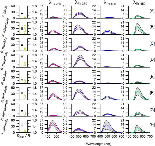
Mean pollen size varied from 20 to 50 μm. Fluorescence intensity emitted from individual particles has long been shown to increase strongly as a function of particle size (e.g., Savage et al. 2017; Sivaprakasam et al. 2011; Hill et al. 2001). Differences in composition between pollen species also play important roles in observed fluorescence intensity, however. For example, P. strobus (Figure 3E) exhibited large mean particle size (52 μm), but weak fluorescence intensity for 280, 405, and 450 nm excitation sources. The mean aspect ratio values of pollen species varied from 1.0 (A. trifida) to 1.6 (A. tridentata), with most species presenting mean values between 1.1 and 1.3.

3.2. Comparison of clustering techniques

3.2.1. Comparison of unsupervised techniques

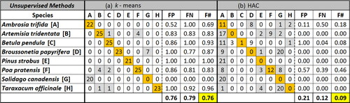
The average accuracy of the k-means algorithm was relatively poor, F value 0.76, and the HAC algorithm showed very poor accuracy, F value 0.09 (Figure 4). This suggests that Euclidian distance between data points (HAC) may not sufficiently separate data in this case. The unsupervised methods consider all variables simultaneously by combining variables, in contrast to supervised methods that randomly sample subsets of the input data. The unsupervised process may result in variables that carry added weight if overlapped between species. Observations with large differences (e.g., a weakly fluorescent particle from one species and a highly fluorescent particle from another) may skew initially developed cluster centroids, making further groupings less accurate by increasing misclassification. As a result of the poor classification results in both cases, it was determined that these techniques would not be sufficient for further analysis.

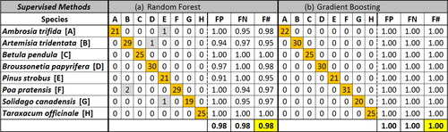
Figure 4. Clustering accuracy (F) comparison utilizing (a) k-means and (b) hierarchical agglomerative clustering algorithms using the entire pollen data set (204 particles). On the left of the dotted lines is a confusion matrix, in which correctly classified particles are highlighted in orange and misclassified particles in gray. On the right side, FP (false positive) represents the number of particles misclassified to that cluster in the vertical dimension, FN (false negative) represents the number misclassified from that cluster in the horizontal dimension, and F represents the harmonic mean of these misclassifications for the cluster. Bottom rows represent mean of all eight species.

3.2.2. Comparison of supervised classifiers

The models developed by the two supervised techniques (RF; F 0.96 and GB; F 1.00) significantly outperformed the two unsupervised techniques, as expected and as summarized in Figure 5. The original training model produced by the GB algorithm classified the data to an average F of 1.00, though this metric can be somewhat misleading because the training data can overfit the data by developing trees that perfectly fit the training data. As a result, the F value of the training dataset can overestimate the true accuracy of the GB model, and the test dataset (discussed below) more accurately represents the separation ability of the model. The RF algorithm has internal checks that reduce its tendency to overfit and so the average accuracy of the training set is almost always lower than for the GB algorithm. The RF algorithm correctly labeled particles in the training set with F of 0.98, corresponding to 2% error or 5 particles misclassified out of 204. In this case one particle from each of three pollen species was misclassified, and two additional P. pratensis particles were misclassified to the A. tridentata cluster. The spectra from these two species are relatively similar (Figure 3A,F), and so misclassification here is reasonable. Because both supervised techniques exhibited relatively high classification accuracy, they were each investigated in more detail.

Figure 5. Clustering accuracy (F) comparison utilizing (a) Random Forest classification and (b) Gradient Boosting classification using the entire pollen data set (204 particles). Figure format analogous to Figure 4.

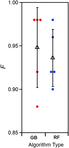
Though the RF and GB algorithms performed well, the developed models may be overfit. Prediction of new, labeled data (e.g., subsets of the data) to the model can thus be important to assess model performance. For both RF and GB, a series of five cross-validation trials were performed with the data sets, where 75% of the randomized data was used to create a training set and the remaining 25% was used as a test set. For most of the trials, RF and GB algorithms performed with similar overall accuracy. Averaged over the five trials, F was 94.8 ± 4.6 for GB and 93.6 ± 3.3 for RF (Figure 6). GB shows higher F than for RF during training, but the mean results are similar following testing. These results imply that GB can overfit the training data despite built-in cross-validation and that RF training sets are more representative classification scenarios. Given the similar results between RF and GB, the similarities between training and testing accuracies exhibited by RF, and the lower computational expense (17x faster), further investigation was limited to the RF algorithm.

Figure 6. Accuracy of GB and RF algorithms summarized after five randomized trials using the 8-species data set. Average accuracy shown as triangle marker. Vertical line shows standard deviation (0.05 for GB, 0.03 for RF). Colored markers show results from individual trials. Identical randomized sets and numerical seeds were used between both algorithms.

3.3. Random Forest variable importance

The relative importance of each portion of each spectrum (770 individual variables accumulated over four emission spectra analyzed at 1 nm resolution) can be determined from the developed RF model as MDG plotted as a function of input variable. Figure 7 thus indicates how each emission curve feature can influence the RF algorithm results. This analysis suggests that the relative importance of the emission spectrum following 280 nm excitation closely follows the pattern of the spectrum itself (Figure 7a). The same is true for the spectrum following 450 nm excitation (Figure 7d), but with overall lower MDG value. The shape of the variable importance curves for the remaining two spectra (Figure 7b,c) present flatter relationships, in some cases with increasing MDG at tails of the spectrum. The shapes of these curves may imply RF model development misled by noise unfiltered by this method, but also suggests that minor features of the spectra may be important for classification, even if not clearly visible in emission spectra averaged from many individual particles. Variable importance measured before data was noise-filtered (as discussed in Section 2.1) is shown in SI Figures S8 and S9. Particle size variables were input as three independent variables (major and minor axes and aspect ratio of particle size). The MDG values summed for these three size variables (input as 3 of 773 variables after noise filtration) totaled only 1% of the total model MDG for the RF model, whereas integrated values for emission curves correspond to 31%, 46%, 18%, and 4% for 280, 350, 405, and 450 nm excitation sources, respectively.

Figure 7. Comparison of variable importance for emission spectra following each excitation wavelength for the RF algorithm. Black traces show MDG value. Colored traces show average fluorescence spectra for Ambrosia trifida (N = 30) shown here as an example (no vertical axis values shown).

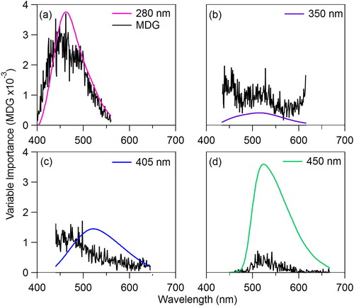
Figure 8. Variable importance (MDG) represented as a fraction of total importance. Wavelength of excitation (λ_Ex) represents sum of emission variables associated with each optical source. Bars sum to 100%. Particle size aspect ratio removed for visual clarity (showed 0% importance).

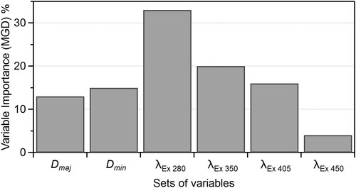
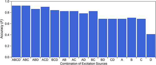
Figure 9. Accuracy of the RF algorithm following fifteen combinations of input variables. Excitation sources represented here as (A) 280 nm, (B) 350 nm, (C), 405 nm_, and (D) 450 nm. All trials consist of a subset of 25% of the particle spectral data predicted to training models from 75% of the data.

Pollen analyses are frequently conducted using particle size and shape analysis, even without any additional information such as spectra (e.g., Weber 2010; Bragg 1969; Jones and Newell 1948). We postulated that developing a model that relies only 1% on physical dimensions of the particles would weaken the classification power of the technique. To counteract the under-representation of particle size within the model, each of the three particle size variables was weighted more heavily in order to increase their influence on the model. By inputting each of three size variables as 33 identical columns of data, the total fraction of input size variables was increased to 99/869 = 11.4%. The weighting factor was chosen arbitrarily so the observed MDG values of the major and minor diameter variables were on the same order of magnitude as the MDG values for emission spectra (e.g., Figure 8). Weighting particle size increased F by a factor of 2.4. Further testing could be conducted on how best to optimize the weighting, but the value utilized was sufficient for the RF model to utilize a mix of particle size and fluorescence information for classification. In this sense, the effect of the scale of weighting used here is less important than its relative effect of arbitrarily increasing particle size importance.

The increased importance of particle size after weighting is shown in Figure S9. Using the weighted particle size inputs, Figure 8 shows that emission spectra following 280 nm excitation exhibit the highest total importance (32% of total MDG), emission spectra following 450 nm excitation are the least important (3%), and the other two emission spectra and particle axes parameters each represent relatively similar influence (15–22%). It is important to note that the values shown in Figure 8 are integrated over full curves in Figure 7 and thus show identical overall trends.

3.4. Instrument simplification

In order to further investigate the relative importance of each of the excitation sources, the mean model accuracy (F) was calculated after removing different combinations of input variables, each associated with a given excitation source. The purpose of this analysis was to investigate the relative loss of sensor functionality if developed with fewer optical excitation sources, thus producing a less expensive and simpler instrument. All combinations of sources were analyzed (16 in total), corresponding to the use of all four sources and the removal of one, two, or three sources. For each of these cases, particle size variables were not input to the model to compare the changes in model accuracy as it applies to spectral data. The results of the analysis are shown for the test set in Figure 9 (results for GB in Figure S10). To simplify discussion, nomenclature here is used such that the 280, 350, 405, and 450 nm sources are labeled as source A, B, C, and D, respectively. For the case using all four excitation sources (case ABCD), the relative accuracy of the model (0.93 training, 0.92 test) was higher than in all cases where at least one source was removed. The test set accuracy for each of four cases where a single source was remove ranged from 0.84 (BCD) to 0.92 (ABC), for the six cases involving two excitation sources from 0.68 (CD) to 0.82 (BC), and for the four cases involving only one source from 0.41 (D) to 0.70 (B). Interestingly, case B showed higher accuracy in both training and trial sets than case BD, implying that the additional input data from the 450 nm source may be confusing model development.

The highest accuracy results from the test set were provided when using all four optical sources (F 0.92), which is not surprising. The comparable accuracy of the ABC (450 nm source removed; F 0.92) and ACD (350 nm source removed; F 0.91) cases suggests here, however, that the relative additional value of either the 350 nm or 450 nm source is marginal toward pollen differentiation. By further simplifying the instrument to use only two sources, the accuracy diminishes somewhat, but all combinations of the 280 nm source (A) plus another source provide relative equal accuracy (0.79–0.82). Interestingly, the BC case (350 and 405 nm sources) provided nearly identical accuracy (0.82) to the cases involving the 280 nm source, whereas the remaining two cases (BD and CD) were substantially lower in accuracy. In cases utilizing only one optical source, the relative accuracy diminished still further, but cases involving the 280, 350, and 405 nm sources were nearly identical, whereas the 450 nm source provided clearly the lowest accuracy results.

The relatively poor performance of the 450 nm source, observed in analyses associated with Figures 7–9 is striking, especially given the ubiquity of emission mode VI in most previously analyzed pollen species (Figure S6). We originally considered that a reason for the lack of importance to this source was influenced by relatively consistent concentrations of fluorophores (e.g., carotenoid compounds) comprising this mode. Figure 3 suggests this is not the case, however, with mean peak emission intensity following 450 nm excitation varying from 2 to 15 arbitrary intensity units. As discussed, the 405 nm source promotes fluorescence from the tails of excitation spectra peaking at ∼450 nm (mode III; phenolics) and ∼520 nm (mode V; carotenoids), and thus are expected to be comprised of emission from both sets of fluorophores. The peak height of emission spectra following 405 nm excitation are lower than spectra following 450 nm excitation for seven of the eight pollen species analyzed here, consistent with the spectra that would be expected if the 405 nm spectra were dominated by mode V (peak emission 520 nm) over mode III (peak emission 450 nm). The relatively low importance of the 450 nm source compared to either the 350 nm or 405 nm sources, however, suggests that the 405 nm excitation gains enough information from mode III to reduce the relative additional value of the 450 nm source.

4. Conclusions

Pollen monitoring and forecasting is relatively expensive and time-consuming due to its manual nature. This leads to poor spatial coverage of measurements sites, further leading to models with relatively poor spatial accuracy. We previously presented the development of a single-particle fluorescence spectrometer designed primarily toward inexpensive, portable, and autonomous differentiation of allergenic pollen and fungal spores. The analysis discussed here shows the application of four types of computational classification to differentiate between properties of individual particles from eight species of commercially acquired pollen. Two commonly used unsupervised clustering methods (k-means and HAC) were investigated, but both methods produced insufficient ability to cluster the pollen species utilized here. We conclude that the GB and RF models provide nearly identical, high accuracy with respect to the pollen species interrogated and that the RF model better optimized cost-benefit with respect to separation accuracy and computational cost. Utilization of these two supervised classifiers requires seeding with supervisory signals from previously identified particles to create suitable models. Measurements of more laboratory or ambient samples will thus require an expansion of both species type and number of particles per species to develop more comprehensive RF models before application to ambient pollen data.

Fluorescence spectra of pollen and other biological aerosol particle types are relatively broad by physical nature and show relatively similar spectral properties between species, thus it has long been suggested that single-particle differentiation between species would be impossible or challenged by high uncertainty (Huffman et al. 2019; Hill et al. 1999). The results here, however, show high levels of separation accuracy using particle size data and well-resolved emission spectra acquired from four excitation sources. In these cases, relatively subtle differences in emission intensity associated with many different chemical compounds present in the pollen are likely why separation can be so effective here. This stands in analogy to other methods that separate, e.g., species of bacteria based on differences in relative proportion of individual lipid molecule concentrations (e.g., Madonna, Voorhees, and Hadfield 2001). For this reason, separation here is improved by the acquisition of relatively high resolution spectra and is thus improved over single-particle techniques that acquire fluorescence emission data in only 1–3 emission channels or with fewer excitation sources.

The analysis of input variables shown here suggests that the 280 nm excitation source is individually the most important of excitation sources utilized (Figures 7 and 8), but that its importance is somewhat diminished when comparing results after removing other individual optical sources from the analysis. It is clear that developing an instrument with all four excitation sources can provide high classification accuracy. Altering the design to utilize three or less source may be an attractive solution, however, to reduce cost and complexity. Of the six two-source cases, three cases (AB, AC, BC) performed approximately equally well. Two of those utilized the 280 nm source, which is not surprising given its overall importance (Figure 8). More surprising was that two of these three cases utilized the 405 nm source, which performed with lower overall integrated importance (Figure 8). In cases where only a single optical source was utilized, the 280, 350, and 405 nm sources performed with similar mean accuracy. From a practical perspective, it is advantageous to choose sources that minimize cost and maximize longevity (e.g., robust, high cumulative operation time) and that provide enough output power density that promote emission spectra sufficiently intense to allow short image integration times. In this context, the 280 nm source is comparatively expensive and provides the weakest output power (0.33 mW compared to 4.5–50 mW for other sources). The weak output power leads to longer exposure times (∼3 min) for images of particle sets compared to the other three sources (3–50 s). For these reasons, a combination of the 350 nm and 405 nm sources (BC) may be ideal for a small detection platform, because demonstrated mean accuracy is high, and both cost and practical convenience are advantageous. In comparison, the addition of the 450 nm source to the 350 and 405 nm sources (BCD) adds only a 2% improvement on the classification, which may not result in sufficient accuracy gain relative to the additional material cost.

The results shown are important not only toward the future development and application of the instrument discussed specifically here, but more broadly to emerging classes of instrumentation that acquire complex data (spectral or otherwise) with many variables toward the purpose of single-bioparticle differentiation. In particular, the analysis of the importance of individual input parameters within a spectrum, integrated groups of variables, and the relative differences in model accuracy after removing instrument components can provide context for development and testing of emerging particle spectrometers. The results shown here will need to be applied to larger datasets, comprising both more pollen species and more particle numbers, in order to more fully test the adequacy of the sensor to pollen identification. The primary purpose here, however, was to provide a computational strategy that can later be utilized in more detail. The application of a much larger set of pollen species was beyond the scope of experimental capabilities at this stage.

The primary goal of the single-particle fluorescence spectrometer discussed here is for the detection of pollen and fungal or mold spore species in approximately real-time, so as to contribute to the areas of missing data and to improve spatial accuracy in forecasting models, e.g., for allergen-containing particles. In this context, the scientific application of the measurement may require species-level identification of all airborne pollen in some cases. In other cases, however, the selective detection of only a few highly allergenic pollen species that dominate the public health response may provide sufficient measurement outcomes. Separation based on different taxonomic groupings may also be advantageous. The expectations with respect to specific applications can thus be modified, and these different scenarios will need to be investigated more fully in subsequent investigations with the sensor as development continues. Toward that end, lowering detection and analysis requirements by collecting lower resolution spectra may be sufficient for adequate prediction. Future analysis will thus investigate the tradeoffs by either collecting spectra at lower resolution or by parameterizing spectra into fewer input variables (e.g., as averaged intensity in the eight fluorophore modes discussed here). For now, however, the computational requirements of the RF model are sufficiently low that it is not expected to be a limiting factor in the particle analysis, and preliminary work suggests that the subtle nuances in the high-resolution spectra as collected contribute positively to accurate pollen differentiation.

Acknowledgments

The authors acknowledge Prof. Emeritus Donald R. Huffman, University of Arizona, for discussions and technical support and Dr. Cathy Durso, University of Denver, for insight on classification and statistical analysis.

Additional information

Funding

Financial support from the University of Denver through a PROF grant, the Phillipson Graduate Fellowship (BES), and the College of Natural Sciences and Mathematics (JAH) is acknowledged.

Notes

1 Term introduced by statistician Corrado Gini.

2 https://www.edmundoptics.com/document/download/352852

References

- Allen, G. P., R. M. Hodgson, S. R. Marsland, and J. R. Flenley. 2008. Machine vision for automated optical recognition and classification of pollen grains or other singulated microscopic objects. 15th International Conference on Mechatronics and Machine Vision in Practice, M2VIP’08, New York, 221–226. doi: 10.1109/MMVIP.2008.4749537.
- American Academy of Allergy Asthma & Immunology. 2019. National Allergy Bureau Pollen Counts. Accessed August 1, 2019. https://www.aaaai.org/global/nab-pollen-counts?ipb=1.
- Blaiss, M. 2010. Allergic rhinitis: Direct and indirect costs. Allergy and Asthma Proceedings, OceanSide Publications.31.3329 doi: 10.2500/aap.2010.
- Bragg, L. H. 1969. Pollen size variation in selected grass taxa. Ecology 50 (1):124–7. doi: 10.2307/1934670.
- Breiman, L. 2001. Random forests. Mach. Learn. 45 (1):5–32. doi: 10.1023/A:1010933404324.
- Buckland, M., and F. Gey. 1994. The relationship between Recall and Precision. J. Am. Soc. Inf. Sci. 45 (1):12–9. doi: 10.1002/(SICI)1097-4571(199401)45:1 < 12::AID-ASI2 > 3.0.CO;2-L.
- Bureau, A., J. Dupuis, B. Hayward, K. Falls, and P. Van Eerdewegh. 2003. Mapping complex traits using random forests. BMC Genet. 4 (Suppl 1):S64. doi: 10.1186/1471-2156-4-S1-S64.
- Buters, J., C. Antunes, A. Galveias, K. Bergmann, M. Thibaudon, C. Galán, C. Schmidt-Weber, and J. Oteros. 2018. Pollen and spore monitoring in the world. Clin. Transl. Allergy 8 (1):9.doi: 10.1186/s13601-018-0197-8.
- Calvo, A., D. Baumgardner, A. Castro, D. Fernández-González, A. Vega-Maray, R. Valencia-Barrera, F. Oduber, C. Blanco-Alegre, and R. Faile. 2018. Daily behavior of urban Fluorescing Aerosol Particles in northwest Spain. Atmos. Environ. 184: 262–77. doi: 10.1016/j.atmosenv.2018.04.027.
- Chen, C., E. A. Hendriks, R. P. W. Duin, J. H. C. Reiber, P. S. Hiemstra, L. A. De Weger, and B. C. Stoel. 2006. Feasibility study on automated recognition of allergenic pollen: Grass, birch and mugwort. Aerobiologia (Bologna) 22 (4):275–84. doi: 10.1007/s10453-006-9040-0.
- Conner, J. K., M. Proctor, P. Yeo, and A. Lack. 1997. The natural history of pollination. Ecology 78 (1):327–239. doi: 10.2307/2266004.
- Crawford, I., S. Ruske, D. Topping, and M. Gallagher. 2015. Evaluation of hierarchical agglomerative cluster analysis methods for discrimination of primary biological aerosol. Atmos. Meas. Tech. 8 (11):4979–91. doi: 10.5194/amt-8-4979-2015.
- Crouzy, B., M. Stella, T. Konzelmann, B. Calpini, and B. Clot. 2016. All-optical automatic pollen identification: Towards an operational system. Atmos. Environ. 140:202–12. doi: 10.1016/j.atmosenv.2016.05.062.
- Dell’Anna, R. (2010). A critical presentation of innovative techniques for automated pollen identification in aerobiological monitoring networks. In Pollen: Structure, types, and effects, ed. B. J. Kaiser, 273–88. Hauppauge, NY: Nova Science Publishers.
- Després, V., Huffman, J. A., Burrows, S., Hoose, C., Safatov, A., Buryak, G., Fröhlich-Nowoisky, J., Elbert, W., Andreae, M., Pöschl, U., and Jaenicke, R. (2012). Primary biological aerosol particles in the atmosphere: a review. Chem. Phys. Meteorol. 64 (1):15598. doi: 10.3402/tellusb.v64i0.15598.
- Dietterich, T. 1995. Overfitting and undercomputing in machine learning. ACM Comput. Surv. 27 (3):326–7. doi: 10.1145/212094.212114.
- Elangasinghe, M. A., N. Singhal, K. N. Dirks, J. A. Salmond, and S. Samarasinghe. 2014. Complex time series analysis of PM10 and PM2.5 for a coastal site using artificial neural network modelling and k-means clustering. Atmos. Environ. 94:106–116. doi: 10.1016/j.atmosenv.2014.04.051.
- Erdmann, N., A. Dell'Acqua, P. Cavalli, C. Grüning, N. Omenetto, J. P. Putaud, F. Raes, and R. V. Dingenen. 2005. Instrument characterization and first application of the single particle analysis and sizing system (SPASS) for atmospheric aerosols. Aerosol Sci. Technol. 39 (5):377–93. doi: 10.1080/027868290935696.
- Erdtman, G. 1952. Pollen morphology and plant taxonomy, GFF. Abingdon: Brill Archive.
- Fennelly, M. J., G. Sewell, M. B. Prentice, D. J. O’Connor, and J. R. Sodeau. 2017. Review: The use of real-time fluorescence instrumentation to monitor ambient primary biological aerosol particles (PBAP). Atmosphere (Basel) 9 (1):1. doi: 10.3390/atmos9010001.
- Forde, E., M. Gallagher, V. Foot, R. Sarda-Esteve, I. Crawford, P. Kaye, W. Stanley, and D. Topping. 2019. Characterisation and source identification of biofluorescent aerosol emissions over winter and summer periods in the United Kingdom. Atmos. Chem. Phys. 19 (3):1665–84. doi: 10.5194/acp-19-1665-2019.
- Frenz, D. A. 1999. Comparing pollen and spore counts collected with the Rotorod Sampler and Burkard spore trap. Ann. Allergy, Asthma Immunol. 83 (5):341–9. doi: 10.1016/S1081-1206(10)62828-1.
- Friedman, J. H. 2001. Greedy function approximation: A gradient boosting machine. Ann. Stat. 29 (5):1189–232. doi: 10.1214/aos/1013203451.
- Gabey, A. M., M. W. Gallagher, J. Whitehead, J. R. Dorsey, P. H. Kaye, and W. R. Stanley. 2010. Measurements and comparison of primary biological aerosol above and below a tropical forest canopy using a dual channel fluorescence spectrometer. Atmos. Chem. Phys. 10 (10):4453–66. doi: 10.5194/acp-10-4453-2010.
- Galán, C., H. García-Mozo, P. Cariñanos, P. Alcázar, and E. Domínguez-Vilches. 2001. The role of temperature in the onset of the Olea europaea L. pollen season in southwestern Spain. Int. J. Biometeorol. 45 (1):8–12. doi: 10.1007/s004840000081.
- Geburek, T., K. Hiess, R. Litschauer, and N. Milasowszky. 2012. Temporal pollen pattern in temperate trees: Expedience or fate? Oikos 121 (10):1603–12. doi: 10.1111/j.1600-0706.2011.20140.x.
- Han, H., X. Guo, and H. Yu. 2017. Variable selection using Mean Decrease Accuracy and Mean Decrease Gini based on Random Forest. Proceedings of the IEEE International Conference on Software Engineering and Service Sciences, IESS, Beijing, 219–224. doi: 10.1109/ICSESS.2016.7883053.
- Hartigan, J. A., and M. A. Wong. 2006. Algorithm AS 136: A K-means clustering algorithm. Appl. Stat. 28 (1):100–8. doi: 10.2307/2346830.
- Healy, D. A., J. A. Huffman, D. J. O'Connor, C. Pöhlker, U. Pöschl, J. R. Sodeau. 2014. Ambient measurements of biological aerosol particles near Killarney, Ireland: A comparison between real-time fluorescence and microscopy techniques. Atmos. Chem. Phys. 14:8055–8069. doi: 10.5194/acp-14-8055-2014.
- Healy, D. A., D. J. O'Connor, A. M. Burke, and J. R. Sodeau. 2012. A laboratory assessment of the Waveband Integrated Bioaerosol Sensor (WIBS-4) using individual samples of pollen and fungal spore material. Atmos. Environ. 60:534. doi: 10.1016/j.atmosenv.2012.06.052.
- Hernandez, M., Perring, A., McCabe, K., Kok, G., Granger, G., and Baumgardner, D. (2016). Chamber catalogues of optical and fluorescent signatures distinguish bioaerosol classes. Atmos. Meas. Tech. 9(7):3283. doi: 10.5194/amt-9-3283-2016.
- Hill, S. C., M. W. Mayo, and R. K. Chang. 2009. Fluorescence of bacteria, pollens, and naturally occurring airborne particles: Excitation/emission spectra. Army Res. Lab. Appl. Phys. (No. ARL-TR-4722): 62.
- Hill, S. C., R. G. Pinnick, S. Niles, N. F. Fell, Y.-L. Pan, J. Bottiger, B. V. Bronk, S. Holler, and R. K. Chang. 2001. Fluorescence from airborne microparticles: dependence on size, concentration of fluorophores, and illumination intensity: erratum. Appl. Opt. 40 (18):3005–3013. doi: 10.1364/AO.40.003005.
- Hill, S., R. Pinnick, S. Niles, and Y. Pan. 1999. Real‐time measurement of fluorescence spectra from single airborne biological particles. F. Anal. 3:221–239. doi: 10.1002/(SICI)1520-6521(1999)3:4/5 < 221::AID-FACT2 > 3.0.CO;2-7.
- Hothorn, T., B. Lausen, A. Benner, and M. Radespiel-Tröger. 2004. Bagging survival trees. Stat. Med. 23 (1):77–91. doi: 10.1002/sim.1593.
- Hothorn, T., A. Zeileis, E. Cheng, and S. Ong. 2015. partykit: A modular toolkit for recursive partytioning in R. J. Mach. Learn. Res. 16 (1):3905–3909.
- Huang, H. C., Y.-L. Pan, S. C. Hill, and R. G. Pinnick. 2011. Fluorescence-based classification with selective collection and identification of individual airborne bioaerosol particles. In Optical Processes in Microparticles and Nanostructures: A Festschrift Dedicated to Richard Kounai Chang on His Retirement from Yale University, , ed. A. Serpengüzel and A. W. Poon, 153–67. Singapore: World Scientific. doi: 10.1142/9789814295789_0009.
- Huffman, J., A. Perring, N. Savage, B. Clot, B. Crouzy, F. Tummon, O. Shoshanim, B. Damit, J. Schneider, V. Sivaprakasam, et al. 2019. Real-time sensing of bioaerosols: Review and current perspectives. Aerosol Sci. Technol. 1–56. doi: 10.1080/02786826.2019.1664724.
- Huffman, D., B. Swanson, and J. A. Huffman. 2016. A wavelength-dispersive instrument for characterizing fluorescence and scattering spectra of individual aerosol particles on a substrate. Atmos. Meas. Tech. 9 (8):3987–3998. 2016. doi: 10.5194/amt-9-3987-2016.
- Huffman, D. R., and Huffman. J. A. 2019. A wavelength dispersive microscope spectrofluorometer for characterizing multiple particles simultaneously. University of Denver. US Patent US20160320306A1. filed January 8, 2014, and issued December 13, 2018
- James, G., D. Witten, T. Hastie, and R. Tibshirani. 2013. An introduction to statistical learning. New York: springer. doi: 10.1007/978-1-4614-7138-7.
- Jones, M. D., and L. C. Newell. 1948. Size, variability, and identification of grass pollen. J. Am. Soc. Agron. 40:136–143. doi: 10.2134/agronj1948.00021962004000020004x.
- Kawashima, S., B. Clot, T. Fujita, Y. Takahashi, and K. Nakamura. 2007. An algorithm and a device for counting airborne pollen automatically using laser optics. Atmos. Environ. 41 (36):7987–7993. doi: 10.1016/j.atmosenv.2007.09.019.
- Kawashima, S., M. Thibaudon, S. Matsuda, T. Fujita, N. Lemonis, B. Clot, and G. Oliver. 2017. Automated pollen monitoring system using laser optics for observing seasonal changes in the concentration of total airborne pollen. Aerobiologia (Bologna) 33 (3):351–362. doi: 10.1007/s10453-017-9474-6.
- Kaye, P., W. R. Stanley, E. Hirst, E. V. Foot, K. L. Baxter, and S. J. Barrington. 2005. Single particle multichannel bio-aerosol fluorescence sensor. Opt. Express 13 (10):3583–3593. doi: 10.1364/OPEX.13.003583.
- Kiselev, D., L. Bonacina, and J. P. Wolf. 2011. Individual bioaerosol particle discrimination by multi-photon excited fluorescence. Opt. Express 19 (24):24516–24521. doi: 10.1364/OE.19.024516.
- Kiselev, D., L. Bonacina, and J. P. Wolf. 2013. A flash-lamp based device for fluorescence detection and identification of individual pollen grains. Rev. Sci. Instrum. 84 (3):033302. doi: 10.1063/1.4793792.
- Knobelspiesse, K. D., C. Pietras, G. S. Fargion, M. Wang, R. Frouin, M. A. Miller, A. Subramaniam, and W. M. Balch. 2004. Maritime aerosol optical thickness measured by handheld sun photometers. Remote Sens. Environ. 93:87–106. doi: 10.1016/j.rse.2004.06.018.
- Könemann, T., F. Ditas, D. Walter, J. Brooks, E. Rodriguez-Caballero, M. Charlotte, M. D. Dewald, F. Drewnick, A. Edtbauer, F. Fachinger, et al. 2019. Online analysis of single aerosol particle fluorescence spectra during the AQABA research cruise around the Arabian Peninsula. Atmos. Chem. Phys. In Preparation.
- Lee, M., O. Yaglidere, and A. Ozcan. 2011. Field-portable reflection and transmission microscopy based on lensless holography. Biomed. Opt. Express 2 (9):2721–2730. doi: 10.1364/BOE.2.002721.
- Liu, Y., Z. Li, H. Xiong, X. Gao, and J. Wu. 2010. Understanding of internal clustering validation measures. Proceedings - IEEE International Conference on Data Mining, ICDM, Sydney, Australia, 911–16. doi: 10.1109/ICDM.2010.35.
- Madonna, A. J., K. J. Voorhees, and T. L. Hadfield. 2001. Rapid detection of taxonomically important fatty acid methyl ester and steroid biomarkers using in situ thermal hydrolysis/methylation mass spectrometry (THM-MS): implications for bioaerosol detection. J. Anal. Appl. Pyrolysis 61 (1-2):65–89. doi: 10.1016/S0165-2370(01)00136-X.
- Miki, K., S. Kawashima, B. Clot, and K. Nakamura. 2019. Comparative efficiency of airborne pollen concentration evaluation in two pollen sampler designs related to impaction and changes in internal wind speed. Atmos. Environ. 203:18–27. doi: 10.1016/j.atmosenv.2019.01.039.
- Mitsumoto, K., K. Yabusaki, K. Kobayashi, and H. Aoyagi. 2010. Development of a novel real-time pollen-sorting counter using species-specific pollen autofluorescence. Aerobiologia (Bologna) 26 (2):99–111. doi: 10.1007/s10453-009-9147-1.
- Mohri, M., A. Rostamizadeh, and A. Talwalkar. 2018. Foundations of machine learning.. Cambridge, MA: MIT press.
- O’Connor, D., D. Healy, S. Hellebust, J. Buters, and J. Sodeau. 2014. Using the WIBS-4 (Waveband Integrated Bioaerosol Sensor) technique for the on-line detection of pollen grains. Aerosol Sci. Technol. 48 (4):341–349. doi: 10.1080/02786826.2013.872768.
- Oteros, J., G. Pusch, I. Weichenmeier, U. Heimann, R. Möller, S. Röseler, C. Traidl-Hoffmann, C. Schmidt-Weber, and J. Buters. 2015. Automatic and online pollen monitoring. Int. Arch. Allergy Immunol. 167 (3):158–166. doi: 10.1159/000436968.
- Pan, Y. L., J. Hartings, R. G. Pinnick, S. C. Hill, J. Halverson, and R. K. Chang. 2003. Single-particle fluorescence spectrometer for ambient aerosols. Aerosol Sci. Technol. 37 (8):628–639. doi: 10.1080/02786820300904.
- Pan, Y. L., S. C. Hill, R. G. Pinnick, J. M. House, R. C. Flagan, and R. K. Chang. 2011. Dual-excitation-wavelength fluorescence spectra and elastic scattering for differentiation of single airborne pollen and fungal particles. Atmos. Environ. 45 (8):1555–1563. doi: 10.1016/j.atmosenv.2010.12.042.
- Pan, Y. L., H. Huang, and R. K. Chang. 2012. Clustered and integrated fluorescence spectra from single atmospheric aerosol particles excited by a 263- and 351-nm laser at New Haven, CT, and Adelphi, MD. J. Quant. Spectrosc. Radiat. Transf. 113 (17):2213–2221. doi: 10.1016/j.jqsrt.2012.07.028.
- Pauling, A., Contributors to the European Aeroallergen Network (EAN), Rotach, M. Gehrig, R. Clot, B. Jäger, S. Cerny, M. Schmidt, R. Bortenschlager, S. Brosch, et al. 2012. A method to derive vegetation distribution maps for pollen dispersion models using birch as an example. Int. J. Biometeorol. 56 (5):949–958. doi: 10.1007/s00484-011-0505-7.
- Percy, D. F., and B. S. Everitt. 2006. Cluster analysis. 3rd ed. J. Oper. Res. Soc. 34:845–846. doi: 10.2307/2584293.
- Perring, A., J. Schwarz, D. Baumgardner, M. Hernandez, D. Spracklen, C. Heald, R. Gao, G. Kok, G. McMeeking, J. McQuaid, et al. 2015. Airborne observations of regional variation in fluorescent aerosol across the United States. J. Geophys. Res. Atmos. 120 (3):1153–1170. doi: 10.1002/2014JD022495.
- Pinnick, R. G., S. C. Hill, Y. L. Pan, and R. K. Chang. 2004. Fluorescence spectra of atmospheric aerosol at Adelphi, Maryland, USA: Measurement and classification of single particles containing organic carbon. Atmos. Environ. 38 (11):1657–1672. doi: 10.1016/j.atmosenv.2003.11.017.
- Pöhlker, C., J. A. Huffman, J.-D. Förster, and U. Pöschl. 2013. Autofluorescence of atmospheric bioaerosols: Spectral fingerprints and taxonomic trends of pollen. Atmos. Meas. Tech. 6 (12):3369–3392. doi: 10.5194/amt-6-3369-2013.
- Pöhlker, C., J. A. Huffman, and U. Pöschl. 2012. Autofluorescence of atmospheric bioaerosols - Fluorescent biomolecules and potential interferences. Atmos. Meas. Tech. 5 (1):37–71. doi: 10.5194/amt-5-37-2012.
- Ranzato, M., P. E. Taylor, J. M. House, R. C. Flagan, Y. LeCun, and P. Perona. 2007. Automatic recognition of biological particles in microscopic images. Pattern Recognit. Lett. 28 (1):31–39. doi: 10.1016/j.patrec.2006.06.010.
- Rebotier, T. P., and K. A. Prather. 2007. Aerosol time-of-flight mass spectrometry data analysis: A benchmark of clustering algorithms. Anal. Chim. Acta doi: 10.1016/j.aca.2006.12.009.
- Richter, R., U. Berger, S. Dullinger, F. Essl, M. Leitner, M. Smith, and G. Vogl. 2013. Spread of invasive ragweed: Climate change, management and how to reduce allergy costs. J. Appl. Ecol. 50 (6):1422–1430. doi: 10.1111/1365-2664.12156.
- Robinson, N., J. Allan, J. Huffman, P. Kaye, V. Foot, and M. Gallagher. 2013. Cluster analysis of WIBS single-particle bioaerosol data. Atmos. Meas. Tech. 6 (2):337–347. doi: 10.5194/amt-6-337-2013.
- Rokach, L. 2010. Ensemble-based classifiers. Artif. Intell. Rev. 33 (1-2):1–39. doi: 10.1007/s10462-009-9124-7.
- Ruske, S., D. Topping, V. Foot, P. Kaye, W. Stanley, I. Crawford, A. Morse, and M. Gallagher. 2017. Evaluation of machine learning algorithms for classification of primary biological aerosol using a new UV-LIF spectrometer. Atmos. Meas. Tech. 10 (2):695–708. doi: 10.5194/amt-10-695-2017.
- Ruske, S., D. O. Topping, V. E. Foot, A. P. Morse, and M. W. Gallagher. 2018. Machine learning for improved data analysis of biological aerosol using the WIBS. Atmos. Meas. Tech. 11 (11):6203–6230. doi: 10.5194/amt-11-6203-2018.
- Šantl-Temkiv, T., F. Carotenuto, B. Sikoparija, T. Maki, P. Amato, M. Yao, P. DeMott, T. Hill, C. Morrism, C. Pöhlker, et al. 2019. Bioaerosol field measurements: Challenges and perspectives in outdoor studies. Aerosol Sci. Technol. 1–27. doi: 10.1080/02786826.2019.1676395.
- Satterwhite, M. B. 1990. Spectral luminescence of plant pollen. 10th Annual International Symposium on Geoscience and Remote Sensing, College Park, MD, 1945–48. doi: 10.1109/igarss.1990.688906.
- Šaulienė, I., L. Šukienė, G. Daunys, G. Valiulis, L. Vaitkevičius, P. Matavulj, S. Brdar, M. Panic, B. Sikoparija, B. Clot, et al. 2019. Automatic pollen recognition with the Rapid-E particle counter: the first-level procedure, experience and next steps. Atmos. Meas. Tech. Discuss 2:1–33. doi: 10.5194/amt-2018-432.
- Sauvageat, E., Y. Zeder, K. Auderset, B. Calpini, B. Clot, B. Crouzy, T. Konzelmann, G. Lieberherr, F. Tummon, and K. Vasilatou. 2019. Real-time pollen monitoring using digital holography. Preprint. doi: 10.5194/amt-2019-427.
- Savage, N., and J. A. Huffman. 2018. Evaluation of a hierarchical agglomerative clustering method applied to WIBS laboratory data for improved discrimination of biological particles by comparing data preparation techniques. Atmos. Meas. Tech. 11 (8):4929–4942. doi: 10.5194/amt-10-4279-2017.
- Savage, N., C. Krentz, T. Könemann, T. Han, G. Mainelis, C. Pöhlker, and J. A. Huffman. 2017. Systematic characterization and fluorescence threshold strategies for the wideband integrated bioaerosol sensor (WIBS) using size-resolved biological and interfering particles. Atmos. Meas. Tech. 10 (11):4279–4302. doi: 10.5194/amt-10-4279-2017.
- Sivaprakasam, V., H. Lin, A. L. Huston, and J. D. Eversole. 2011. Spectral characterization of biological aerosol particles using two-wavelength excited laser- induced fluorescence and elastic scattering measurements. Opt. Express 19 (7):6191–6208. doi: 10.1364/OE.19.006191.
- Songnuan, W. 2013. Wind-pollination and the roles of pollen allergenic proteins. Asian Pacific J. Allergy Immunol. 31 (4):261. doi: 10.12932/AP0287.31.4.2013.
- Stach, A., M. Smith, J. C. Prieto Baena, and J. Emberlin. 2008. Long-term and short-term forecast models for Poaceae (grass) pollen in Poznań, Poland, constructed using regression analysis. Environ. Exp. Bot. 62 (3):323–332. doi: 10.1016/j.envexpbot.2007.10.005.
- Strobl, C., A.-L. Boulesteix, A. Zeileis, and T. Hothorn. 2007. Bias in random forest variable importance measures: illustrations, sources and a solution. BMC Bioinform. 8 (1):25. doi: 10.1186/1471-2105-8-25.
- Swanson, B., and J. A. Huffman. 2018. Development and characterization of an inexpensive single-particle fluorescence spectrometer for bioaerosol monitoring. Opt. Express 26 (3):3646–3660. doi: 10.1364/OE.26.003646.
- Tello-Mijares, S., and F. Flores. 2016. A novel method for the separation of overlapping pollen species for automated detection and classification. Comput. Math. Methods Med. 2016:1–12. doi: 10.1155/2016/5689346.
- Tseng, Y.-T., and S. Kawashima. 2019. Applying a pollen forecast algorithm to the Swiss Alps clarifies the influence of topography on spatial representativeness of airborne pollen data. Atmos. Environ. 212:153–162. doi: 10.1016/j.atmosenv.2019.05.052.
- Weber, R. W. 2010. Pollen identification. Ann. Allergy, Asthma Immunol. 80 (2):141–148. doi: 10.1016/S1081-1206(10)62947-X.
- Wlodarski, M., M. Kaliszewski, M. Kwasny, K. Kopczynski, Z. Zawadzki, Z. Mierczyk, J. Mlynczak, E. Trafny, and M. Szpakowska. 2006. Fluorescence excitation-emission matrices of selected biological materials. Optically Based Biological and Chemical Detection for Defence III, Stockholm, Sweden, 639806. doi: 10.1117/12.687872.
- Wu, Y., A. Calis, Y. Luo, C. Chen, M. Lutton, Y. Rivenson, X. Lin, H. C. Koydemir, Y. Zhang, H. Wang, et al. 2018. Label-free bioaerosol sensing using mobile microscopy and deep learning. ACS Photonics 5 (11):4617–4627. doi: 10.1021/acsphotonics.8b01109.
- Zhu, W., Q. Liu, and Y. Wu. 2015. Aerosol absorption measurement at SWIR with water vapor interference using a differential photoacoustic spectrometer. Opt. Express 23 (18):23108–23116. doi: 10.1364/OE.23.023108.