Numerical simulation of aerosol dynamics in an impinging jet with microdroplet coalescence

Abstract

Droplet laden jet plays important roles in cutting-edge technologies including spray cooling, aerosol jet printing, pollution control, and cascade impactors. In this work, a numerical simulation scheme for jet flow is proposed. The turbulence is calculated based on the $\overline{v^2}$-f model and the droplets are described by the discrete phase model. The droplet-droplet collisions are calculated by a mesh-independent collision model. The results are compared with an experiment in which concentric dual-ring deposition patterns were observed on the impinging plate. The effects of the droplet volume fraction are investigated. Criteria for the necessity of two-way coupling as well as coalescence calculation are provided. This work provides a practical tool for aerosol impinging research and design.

Copyright © 2020 American Association for Aerosol Research

EDITOR:

• Yannis Drossinos

Introduction

Impinging jets have received considerable attention in many industrial applications, including heat transfer, manufacturing, pollution control and jet printing. Numerous studies focused on the heat transfer process of droplet impingement (Jambunathan et al. 1992; Zuckerman and Lior 2006) and performance of aerosol impactors which have been widely used in environmental studies and industrial processes (Arffman, Marjamäki, and Keskinen 2011; Chen et al. 2016; Marple et al. 2014; Mottaghi, Abbasalizadeh, and Ahmady-Birgani 2019). However, accurate understanding and modeling of the jet and impingement processes are still challenging. For example, the cascade impactors have a significant error when the aerosol mass concentration is large enough such that the agglomeration/coalescence among the particles/droplets cannot be neglected (Blomquist, Strom, and Stromquist 1984). Similar problems exist in aerosol jet printing which can achieve a resolution as fine as 10 µm (Tait et al. 2015; Feng and Renn 2019). The challenge is to control the droplet motion to obtain the well-defined edges which need an accurate prediction of deposit positions (Feng 2018; Jones et al. 2010; Mette et al. 2007).

Droplet impingement and deposition have been extensively studied for droplets larger than 20 µm (Andreassi, Ubertini, and Allocca 2007; Mundo, Sommerfeld, and Tropea 1995). For droplets/particles of smaller than 20 µm, many researchers have studied the impaction behavior with circular jets for its application in aerosol particle size classification with the cascade impactors (Andersen 1966; Marple et al. 1986). The experimental results are quite limited due to the difficulties in size control and in-situ observation. Liu et al. (2010) observed the deposition of micron liquid droplets in impinging jet and observed a dual-ring deposition pattern experimentally. Zhao et al. (2012) found the ink droplets formed two peaks in the printed line. The mechanisms of the dual-ring deposition pattern were explained based on velocity field and skin fraction field by Liu et al. (2010). The deposition pattern was affected by collisions and coalescences among droplets, which was difficult to directly observe in the experiment (Liu et al. 2010). Mottaghi, Abbasalizadeh, and Ahmady-Birgani (2019) investigated the particle deposition pattern of a multi-nozzle impactor experimentally and numerically and found the sphericity, diameter, and shape of the particle have strong effects on the deposition. Recently, Feng and Renn (2019) provided an overview pointing out suitable droplet diameter range and jet Reynolds number window for aerosol jet printing, calling for an accurate numerical simulation scheme.

Simulation is an alternative approach which avoids in-situ experimental difficulties. For the flow field calculation, direct numerical simulation (DNS), large eddy simulation (LES) and Reynolds-averaged Navier-Stokes (RANS) models have been employed for impinging flows (Jaramillo et al. 2012; Satake and Kunugi 1998; Mottaghi, Abbasalizadeh, and Ahmady-Birgani 2019). Feng (2017) studied the micro-particle deposition patterns from a circular jet. The effects of taper angle of the nozzle and jet-to-plate distance were evaluated. His studies focused on the laminar flow and the study did not consider the inter-particle collision. Jaramillo et al. (2012) applied DNS and RANS models to calculate the temperature and flow fields of a turbulent plane impinging jet at Re = 20000. DNS was compared to the explicit algebraic Reynolds stress models and linear and non-linear eddy viscosity models in conjunction with k-ε and k-ω platforms. Results showed that these RANS models successfully predicted the local Nusselt number at the stagnation region but failed to capture the downstream local Nusselt number profile. DNS and LES are expensive in computational cost, rarely applicable for industrial applications especially in high Reynolds number cases (Tian and Ahmadi 2007). RANS remains popular for industrial applications with the solution variables in the instantaneous Navier-Stokes equations being decomposed into the ensemble-averaged or time-averaged and fluctuating components. Among RANS, Behnia et al. (1999) showed that the $\overline{v^2}$-f model is suitable in flow field calculation for impinging jets.

The droplets/particles could also have an influence on the carrying gas flow field, therefore two-way coupling may be necessary. For particles of around 100 µm diameter, Elghobashi (1994) recommended that one-way coupling is enough when the particle volume fraction is smaller than 10⁻⁶, and two-way coupling method is necessary when the fraction is larger than 10⁻⁶. However, the criteria for aerosol particles with diameters less than 5 µm is still an open question.

Collisions may occur among the droplets/particles and induce coalescence/agglomeration. Lagrangian discrete phase model has been employed for the dilute case (Tian and Ahmadi 2007). A stochastic approach for droplet collisions with a probability-based algorithm was proposed by O’Rourke (1981), which has been widely used in industry. However, this method is time-consuming and manifests mesh dependency because collisions are supposed to happen in the same cell (Li et al. 2006; Schmidt and Rutland 2000). Zhang, Mi, and Wang (2012) developed a mesh-independent model considering the collisions in different cells to solve the defect. For turbulence-induced agglomeration, fictitious collision partners were used by Oesterle and Petitjean (1993) and Anh Ho and Sommerfeld (2002). Xu, Shen, and Wang (2015) proposed a turbulence agglomeration model based on the mesh-independent model proposed by Zhang, Mi, and Wang (2012), which searched for real collision pairs with turbulent collision kernels to get the collision frequencies.

This work reproduces the dual-ring deposition pattern in the droplet-laden impingement jet numerically, and then proposes criteria for the necessity of two-way coupling and collision modeling in the simulation of impinging jet. The modeling together with the criteria provides a practical tool for the analysis of various aerosol applications like spay cooling, aerosol cascade impactor, and jet printing.

Model description

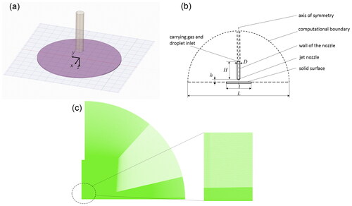
The simulation system is set according to the experiment by Liu et al. (2010) in which a single turbulent impinging aerosol jet was studied and a dual-ring deposition pattern was observed. As Figure 1a shows, the jet flow is set vertically downwards and it impinges orthogonally onto a flat plate. The carrying gas and the aerosol droplets enter through the inlet and mix in the pipe. The Reynolds number is 19300 based on the inlet mean velocity, v_in, and diameter of the nozzle, D.

Figure 1. Simulation schematic of the impinging jet with micron and submicron droplets: (a) 3D sketch; (b) scale and boundary conditions; (c) mesh setup.

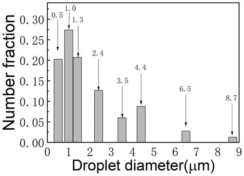
The material of droplet is set as olive oil with density ρ = 920 kg/m³, surface tension σ = 3.2 × 10⁻² N/m, viscosity µ = 8.1 × 10⁻² Ns/m², and environment temperature T is 298 K. The size distribution of the inject droplets is shown in Figure 2. In the simulation, the disk diameters, d_disk, in the experiments have been converted into the spherical diameter, d_d, according to the relationship d_d = d_disk/2.3 proposed by Mundo, Sommerfeld, and Tropea (1995). In the experiment of Liu et al. (2010), the numbers of droplets were counted in 40 groups, shown in Figure S4 in the online supplementary information (SI). To simplify the calculation, these 40 groups are combined into 8 big groups. And the average diameter (Sauter mean diameter, SMD) in each group is set as the typical size. The SMD of the inject droplet is 4.85 µm. The number concentration of the droplets at the exit c₁ was 1.94 × 1013/m³ and the volume fraction was 1.02 × 10⁻⁵ in the experiment (Liu et al. 2010). To analyze the influence of the droplet concentration, five different volume fractions are studied. From low to high they are α_V0.1 = 0.1α_V1, α_V1 = 1.02 × 10⁻⁵ which is identical to the experiment, α_V2 = 2α_V1, α_V4 = 4α_V1, and α_V8 = 8α_V1.

Figure 2. Size distribution of the injected micro and nano droplets. The average diameter (Sauter mean diameter) of the droplets is 4.85 µm.

A two-dimensional axisymmetric geometry is set up as the computational domain. The axis of the symmetry is shown in Figure 1b. The inlet is set as a velocity inlet and the inlet velocity, v_in, is 30 m/s. The outer boundaries of the simulation domain are set as pressure outlet for the continuous phase and escape condition for the discrete phase. For droplet-wall interaction, the plate is set as a trap condition, which means no rebound for droplets. Mundo, Sommerfeld, and Tropea (1995) showed that the critical velocity for rebounding is more than 30 m/s for droplets with diameters smaller than 10 µm. The Weber number in this research $We= {\rho }_d{d}_d{\overline{u_d}}^2/\sigma$ is less than 125, researchers (Šikalo, Tropea, and Ganić 2005; Wang et al. 2016; Wierzba 1990; Zhang et al. 2014) have suggested that there was no splashing or rebound for this small We. The no-slip boundary condition is imposed for the fluid on the walls.

Computational schemes

As depicted in Figure 1c, a 2D non-uniform mesh with 202,507 quadrilateral cells with a higher resolution near the solid boundaries is used. The mesh independence has been validated by refining the mesh by 1.2 times in both axial and radial directions. The differences between 2D and 3D meshes have been assessed in the SI. 2D simulation is time-saving but the random fluctuations existing in the circumferential direction may not be captured in the 3D system. Commercial software ANSYS Fluent in double precision is applied for the simulation. The turbulence is calculated by $\overline{v^2}$-f model. Droplet trajectory analysis is conducted using the discrete phase model (DPM) and the collisions among droplets are calculated using user-defined function (Tian and Ahmadi 2007; Zhang, Mi, and Wang 2012). The spatial discretization of the gradient is Least squares cell-based scheme. The spatial discretization methods of turbulent kinetic energy, turbulent dissipation rate, velocity variance scales, and elliptic relaxation function are the third order Monotone Upstream-Centered Schemes for Conservation Laws. The first grid point is at y⁺ ≈ 1.

For the continuous phase, the incompressible Navier-Stokes equations are solved to get the flow structures. Equations (1)(1) $$\frac{\partial \rho }{\partial t}+\frac{\partial }{\partial x_i}\left(\rho \overline{u_i}\right)=0$$(1) and (2)(2) $$\frac{\partial }{\partial t}\left(\rho \overline{u_i}\right)+\frac{\partial }{\partial x_i}\left(\rho \overline{u_i}\overline{u_j}\right)=-\frac{\partial p}{\partial x_i}+\frac{\partial }{\partial x_j}\left[\mu \left(\frac{\partial \overline{{\mathrm{u}}_i}}{\partial x_j}+\frac{\partial \overline{u_j}}{\partial x_i}-\frac{2}{3}{\delta }_{ij}\frac{\partial \overline{u_i}}{\partial x_i}\right)\right]+\frac{\partial }{\partial x_j}(-\rho \overline{u{\mathrm{\prime }}_{i}u{\mathrm{\prime }}_j})$$(2) are the Cartesian tensor form of RANS equations, in which the velocities and other variables are represented as the time-averaged values: (1) $$\frac{\partial \rho }{\partial t}+\frac{\partial }{\partial x_i}\left(\rho \overline{u_i}\right)=0$$(1) (2) $$\frac{\partial }{\partial t}\left(\rho \overline{u_i}\right)+\frac{\partial }{\partial x_i}\left(\rho \overline{u_i}\overline{u_j}\right)=-\frac{\partial p}{\partial x_i}+\frac{\partial }{\partial x_j}\left[\mu \left(\frac{\partial \overline{{\mathrm{u}}_i}}{\partial x_j}+\frac{\partial \overline{u_j}}{\partial x_i}-\frac{2}{3}{\delta }_{ij}\frac{\partial \overline{u_i}}{\partial x_i}\right)\right]+\frac{\partial }{\partial x_j}(-\rho \overline{u{\mathrm{\prime }}_{i}u{\mathrm{\prime }}_j})$$(2) where ρ is the density of the fluid, t time, µ the dynamic viscosity, and $\overline{u}$ the velocity of fluid. Subscript i stands for the component of x direction, j for the component of y direction. δ_ij is the Kronecker delta, which means that if i = j, δ_ij= 1, if i ≠ j, δ_ij = 0.

In Equation (2)(2) $$\frac{\partial }{\partial t}\left(\rho \overline{u_i}\right)+\frac{\partial }{\partial x_i}\left(\rho \overline{u_i}\overline{u_j}\right)=-\frac{\partial p}{\partial x_i}+\frac{\partial }{\partial x_j}\left[\mu \left(\frac{\partial \overline{{\mathrm{u}}_i}}{\partial x_j}+\frac{\partial \overline{u_j}}{\partial x_i}-\frac{2}{3}{\delta }_{ij}\frac{\partial \overline{u_i}}{\partial x_i}\right)\right]+\frac{\partial }{\partial x_j}(-\rho \overline{u{\mathrm{\prime }}_{i}u{\mathrm{\prime }}_j})$$(2) , the Reynolds stresses $-\rho \overline{u{\prime }_{i}u{\prime }_j}$ can be expressed by different turbulent models. The standard k-ε, RNG k-ε, realizable k-ε, $\overline{v^2}$-f model and Reynolds Stress Model (RSM) have been applied in the industry application (Angioletti, Nino, and Ruocco 2005; Behnia, Parneix, and Durbin 1998; Durbin 1993; Durbin 2018; Jaramillo et al. 2012; Wu, Xu, and Wang 2018). The standard k-ε is widely used in engineering since it needs low computational cost to predict the turbulence flow structure. However, it assumes that the turbulent viscosity is an isotropic scalar quantity which may not be suitable in near wall region (Ghadimi, Yousefifard, and Nowruzi 2017). The standard or modified k-ε models have been validated for flows parallel to the wall but not for jet impingement on a solid plate. Craft, Graham, and Launder (1993) showed that the k-ε model is not suitable for heat transfer prediction in a non-confined impinging jet. The RSM abandons the isotropic eddy-viscosity hypothesis to overcome standard k-ε model’s defect but the computational cost is higher than the standard k-ε model and $\overline{v^2}$-f model.

In this work, the turbulence is calculated based on the $\overline{v^2}$-f model. The $\overline{v^2}$-f model is a four-equation model based on transport equations for the turbulence kinetic energy (k), its dissipation rate (ε), a velocity variance scale ($\overline{v^2}$), and elliptic relaxation function (f). The transport equations are: (3) $$\frac{\partial }{\partial t}\left(\rho k\right)+\frac{\partial }{\partial x_i}\left(\rho k\overline{u_i}\right)=P-\rho \epsilon +\frac{\partial }{\partial x_j}\left[\left(\mu +\frac{{\mu }_t}{{\sigma }_k}\right)\frac{\partial k}{\partial x_j}\right]+S_k$$(3) (4) $$\frac{\partial }{\partial t}\left(\rho \epsilon \right)+\frac{\partial }{\partial x_i}\left(\rho \epsilon \overline{u_i}\right)=\frac{C{\mathrm{\prime }}_{\epsilon 1}P-C_{\epsilon 2}\rho \epsilon }{T}+\frac{\partial }{\partial x_j}\left[\left(\mu +\frac{{\mu }_t}{{\sigma }_{\epsilon }}\right)\frac{\partial \epsilon }{\partial x_j}\right]+S_{\epsilon }$$(4) (5) $$\frac{\partial }{\partial t}\left(\rho \overline{v^2}\right)+\frac{\partial }{\partial x_i}\left(\rho \overline{v^2}\overline{u_i}\right)=\rho kf-6\rho \overline{v^2}\frac{\epsilon }{k}+\frac{\partial }{\partial x_j}\left[\left(\mu +\frac{{\mu }_t}{{\sigma }_k}\right)\frac{\partial \epsilon }{\partial x_j}\right]+S_{\overline{v^2}}$$(5) (6) $$f-L^2\frac{{\partial }^{2}f}{\partial x_j^2}=(C_1-1)\frac{2/3-\overline{v^2}/k}{T}+C_1\frac{P}{\rho k}+\frac{5\overline{v^2}/k}{T}+S_f$$(6) where $P=2{\mu }_t{S}^2,$$S^2={\mathrm{S}}_{\text{ij}}{S}_{\text{ij}},$$S_{\text{ij}}=\frac{1}{2}\left(\frac{\partial \overline{u_i}}{\partial x_j}+\frac{\partial \overline{u_j}}{\partial x_i}\right),$ and the turbulent time scale T are defined by (7) $$T=\min \left[\max \left[\frac{k}{\epsilon },6\sqrt{\frac{\nu }{\epsilon }}\right],\frac{\alpha }{\sqrt{3}}\frac{k}{\overline{v^2}{C}_{\mu }\sqrt{2S^2}}\right]$$(7) (8) $$L=C_L\mathrm{\hspace{0.17em}max}\left[\min \left[\frac{k^{3/2}}{\epsilon },\frac{1}{\sqrt{3}}\frac{k^{3/2}}{\overline{v^2}{C}_{\mu }\sqrt{2S^2}}\right],C_{\eta }{\left(\frac{{\nu }^3}{\epsilon }\right)}^{1/4}\right]$$(8)

In the above equations, $\alpha$ = 0.6, C₁ = 1.4, C₂ = 0.3, $C_{\epsilon 1}$ = 1.4, $C_{\epsilon 2}$= 1.9,$C_{\eta }$= 70,$C_{\mu }$= 2.2,$C_L$= 0.23, ${\sigma }_k$= 1,${\sigma }_{\epsilon }$= 1.3, $C{\mathrm{\prime }}_{\epsilon 1}=C_{\epsilon 1}\left(1+0.045\sqrt{k/\overline{v^2}}\right),$ $S_k,$ $S_{\epsilon },$ $S_{\overline{v^2}}$ and $S_f$ are source terms and $\nu$ is the kinematic viscosity. The $\overline{v^2}$-f model takes the near-wall turbulence anisotropy into consideration. It is a simplification of the full Second Moment Closure (SMC) model, avoiding computational stability problems in the full SMC model by solving the mean flow with an eddy viscosity. The essential feature of the $\overline{v^2}$-f model is that velocity scale $\overline{v^2}$ instead of k is applied to evaluate the turbulent viscosity. $\overline{v^2}$ is proportional to k far from solid walls, while in the near-wall region, it becomes the velocity fluctuation normal to the wall. k fails to represent the damping of turbulent transport close to the wall while normal velocity fluctuations can provide the right result. More details are outlined by Behnia et al. (1999).

Droplets are treated as the discrete phase. The rotation of droplets is neglected. The trajectories are calculated in a Lagrangian reference frame by integrating the forces on the droplets: (9) $$\frac{d\overrightarrow{u_d}}{dt}=F_D\left(\overrightarrow{u}-\overrightarrow{u_d}\right)+\frac{\overrightarrow{g}({\rho }_d-\rho )}{{\rho }_d}+\overrightarrow{F}$$(9) where $\overrightarrow{u_d}$ is the velocity of droplet, $\overrightarrow{u}$ is the velocity of fluid, $\overrightarrow{g}$ is the gravity, ρ_d is the density of the droplet, ρ is the density of the fluid, and t is the time. $F_D\left(\overrightarrow{u}-\overrightarrow{u_d}\right)$ is the drag force (force/unit droplet mass).

For droplets smaller than 2 µm, Stokes-Cunningham drag law has been shown to be valid (Ounis, Ahmadi, and McLaughlin 1991). F_D can be expressed as: (10) $$F=\frac{18\mu }{{\rho }_d{d}_d^2{C}_c}$$(10) where µ is the dynamic viscosity of the fluid, d_d the droplet diameter. C_c is the Cunningham correction factor to Stokes drag law and can be computed from (11) $$C=1+\frac{2\lambda }{d_d}(1.257+0.4e^{-(1.1d_d/2\lambda )})$$(11) where λ is the molecular mean free path.

For droplet bigger than 2 µm, (12) $$F=\frac{3\mu C_{D}R{e}_d}{4{\rho }_d{d}_d^2}$$(12)

Re_d is the relative Reynolds number based on the diameter of the droplets and the relative velocity between the fluid and the droplet. C_D=a₁+ a₂/Re_d+ a₃/Re_d², where a₁, a₂, a₃ are constants that apply to droplets over several ranges of Re_d given by Morsi and Alexander (1972) and the reader can refer to the SI. $\overrightarrow{F}$ is an additional acceleration force. Ounis, Ahmadi, and McLaughlin (1991) showed that for micro-droplets, Brownian motion is important, while virtual mass force, Basset history force, Saffman force, and Magnus force could be negligible.

The effect of the instantaneous turbulent velocity fluctuation on the droplet motion is considered by the stochastic tracking model. When calculating the trajectories of the droplets, the velocity of fluid is $\overrightarrow{u}=\overrightarrow{\overline{u}}+\overrightarrow{u}\mathrm{\prime },$ where $\overrightarrow{\overline{u}}$ is the mean fluid phase velocity and the $\overrightarrow{u}\mathrm{\prime }$ is the instantaneous fluid velocity. $\overrightarrow{u}\mathrm{\prime }$ is calculated by discrete random walking (DRW) model (Gosman and Loannides 1983), which has already been implemented in ANSYS Fluent. In the DRW model, $\overrightarrow{u}\mathrm{\prime }$ is a Gaussian distributed random velocity fluctuation, $\overrightarrow{u}\mathrm{\prime }\left(x,y,z\right)=({\zeta }_x\sqrt{\overline{{\overrightarrow{u}\mathrm{\prime }\left(x\right)}^2}},{\zeta }_y\sqrt{\overline{{\overrightarrow{u}\mathrm{\prime }\left(y\right)}^2}},{\zeta }_z\sqrt{\overline{{\overrightarrow{u}\mathrm{\prime }\left(z\right)}^2}})$ where ${\zeta }_x,$ ${\zeta }_y,$ ${\zeta }_z$ are normally distributed random numbers. In this simulation, the flow field is calculated by $\overline{v^2}$-f model, an anisotropic turbulence model. While calculating the trajectories of the droplets, the isotropy is assumed and $\sqrt{\overline{{\overrightarrow{u}\mathrm{\prime }\left(x\right)}^2}}=\sqrt{\overline{{\overrightarrow{u}\mathrm{\prime }\left(y\right)}^2}}=\sqrt{\overline{{\overrightarrow{u}\mathrm{\prime }\left(z\right)}^2}}=\sqrt{2k/3}.$ Other models like particle cloud model (Litchford and Jeng 1991) are also proposed to consider the turbulence effect, and it is rather complex and should be studied further.

The two-way coupling is implemented by alternately solving the discrete phase and continuous phase equations until the solutions in both phases have stopped changing, which is provided by ANSYS Fluent. In this simulation, only the momentum transfer from droplets to the fluid was considered while the heat and mass transfer were neglected. The momentum transfer was computed by examining the change in momentum of a droplet as it passed through each control volume. The force from the discrete phase to the fluid is computed as (13) $$\overrightarrow{F_{df}}=\sum \overrightarrow{F_d}\dot{m}\mathrm{\Delta }t$$(13) where $\mathrm{\Delta }t$ is time step, $\dot{m}$ is the mass flow rate of the droplets. $\overrightarrow{F_d}$ is (14) $$\overrightarrow{F_d}=\left\{\begin{array}{c}\frac{3\mu C_D{Re}_d}{4{\rho }_d{d}_d^2}\left(\overrightarrow{u_d}-\overrightarrow{u}\right), d_d\ge 2\mathrm{\mu m}\\ \frac{18\mu }{{\rho }_d{d}_d^2{C}_C}\left(\overrightarrow{u_d}-\overrightarrow{u}\right), d_d<2\mathrm{\mu m}\end{array}\right.$$(14)

For droplet collisions, a mesh-independent collision model base on Zhang, Mi, and Wang (2012) is applied. The inter-particle/droplet collision frequency depends on the kinetic theory of the gases is defined by the following equation: (15) $$f=\frac{n\pi (r_1+r_2{)}^2{v}_{\mathit{rel}}}{V_c}=n_d\pi (r_1+r_2{)}^2{v}_{\mathit{rel}}=n_{d}K$$(15) where r₁ and r₂ are the radii of the two droplets that may collide, v_rel is the relative velocity of two particles, n_d = n/V_c is the droplets number density in the respective control volume. K is defined as the collision kernel. According to the kinetic theory, the collision frequency can be calculated by Equation (15)(15) $$f=\frac{n\pi (r_1+r_2{)}^2{v}_{\mathit{rel}}}{V_c}=n_d\pi (r_1+r_2{)}^2{v}_{\mathit{rel}}=n_{d}K$$(15) . However, for the droplets in turbulent flow, v_rel should be modified due to Brownian coagulation and turbulent effect. In the simulation, some developed collision kernels are applied to calculate the collision probability.

In this study, the Knudsen number, Kn, is smaller than 1. In the continuum and near-continuum regime, the Brownian motion-induced collision kernel is given by Otto et al. (1999) (16) $$K_{\mathit{Brownian}}=\frac{2k_{b}T}{3\mu }(\frac{C_c\left(r_1\right)}{r_1}+\frac{C_c\left(r_2\right)}{r_2})(r_1+r_2)$$(16) where k_b is Boltzmann constant and C_c(r) is the Cunningham slip factor in Equation (11)(11) $$C=1+\frac{2\lambda }{d_d}(1.257+0.4e^{-(1.1d_d/2\lambda )})$$(11) . In this simulation, C_c(r) is set as 1 for the mean diameter of the droplet is around 5 µm. For smaller droplets, C_c(r) can be calculated by Equation (11)(11) $$C=1+\frac{2\lambda }{d_d}(1.257+0.4e^{-(1.1d_d/2\lambda )})$$(11) .

Turbulent collision kernels have been studied extensively (Saffman and Turner 1956; Sommerfeld 2001; Wang, Wexler, and Zhou 2000). In this simulation, the turbulent collision kernel is selected according to the droplet Stokes number (Meyer and Deglon 2011; Zhou, Wexler, and Wang 2001). The gravity, turbulent shear, and turbulent acceleration are considered (Wang, Wexler, and Zhou 1998): (17) $$K_{\mathit{turb}}=\sqrt{8\pi }{(r_1+r_2)}^2\left[\frac{1}{15}{\Gamma }^2(r_1+r_2{)}^2+{\left(1-\frac{{\rho }_f}{{\rho }_d}\right)}^2{\left({\tau }_d\left(r_1\right)-{\tau }_d\left(r_2\right)\right)}^2\left(1.3{\left(\eta \Gamma \right)}_{}^2+\frac{\pi }{8}{g}^2\right)\right]$$(17) where $\Gamma$ is the Kolmogorov shear rate, which can be calculate by $\Gamma =\sqrt{\epsilon \rho /\mu }.$ ${\left(\eta \Gamma \right)}_{}^2$ is the turbulent acceleration experienced by droplets much smaller than the Kolmogorov length scale, g is the gravitational acceleration.

The processes of turbulent coagulation and Brownian coagulation can be assumed to be statistically independent (Zaichik and Solov’ev 2002). Therefore, the collision kernel K_all considering the Brownian motion and the turbulent effect is (18) $$K_{\mathit{all}}={\left(K_{\mathit{Browni}\mathrm{a}n}^2+K_{\mathit{turb}}^2\right)}^{1/2}$$(18)

When two droplets collide, the outcome can be coalescence, bounce and fragmentation. O’Rourke (1981) provided a criterial b_crit to determine the collision outcome: (19) $$b_{\mathit{crit}}=(r_1+r_2)\sqrt{\min (1.0,\frac{2.4fr}{We})}$$(19) where fr is defined as fr(r₁/r₂) = (r₁/r₂)³ − 2.4 (r₁/r₂)² + 2.7 (r₁/r₂). And the actual collision parameter b is calculated by (20) $$b=(r_1+r_2)\sqrt{Y}$$(20) where Y is a random number between 0 and 1. If b <b_crit, a coalescence happens. Otherwise, a bounce happens.

Zhang, Mi, and Wang (2012) showed that when the number of droplet parcels in a cell, ψ, is greater than 10, the error due to mesh dependence is small enough. In the mesh-independent model, a physically reliable volume V_pr is applied instead of the mesh cell volume V_c. A sphere with the volume equal to V_pr is generated and the parcel position is set as its center. The droplets distribute uniformly in the sphere and thus the search of collisions is conducted in the sphere. V_pr could be obtained as V_pr = n/c_pr, where n is the droplet number in the parcel. c_pr is the local droplet number density and could be calculated by the current cell and the neighbor cells. (21) $$c_{pr}={\sum }_{\mathit{loc}}n/{\sum }_{\mathit{loc}}{V}_c$$(21) where loc is the local cells within a distance of l. In this study, l is the distance satisfying ψ = 10 and other details can refer to Zhang, Mi, and Wang (2012).

Results

Jet flow field

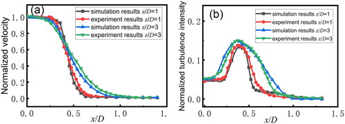
The performance of $\overline{v^2}$-f model on flow field calculation is evaluated by comparing simulation results with the experimental results by Liu et al. (2010). The diameter of the jet nozzle is 9.5 mm and the jet exit velocity is 30 m/s. Figure 3a shows the mean velocity profiles normalized by the local maximum velocity and Figure 3b shows the turbulence intensity normalized by the central exit velocity. The definition for the turbulence intensity, I, is $I=u^{\prime }/\overline{u}.$ As for calculation, $I=\sqrt{2/3k}/\overline{u}$ is used in this study. x is the distance to the centerline in radial direction and z is the distance to the nozzle in streamwise direction and D is the diameter of the nozzle. The comparison shows the fair performance of $\overline{v^2}$-f model in the flow field calculation.

Figure 3. Normalized velocity profiles and turbulence intensity in simulation compared with the experiment: (a) normalized velocity profile at z/D = 1 and z/D = 3; (b) normalized turbulence intensity at z/D = 1 and z/D = 3. z is the distance to the nozzle in streamwise direction and x is the distance to the centerline in radial direction.

Impinging deposition

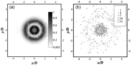
The dual-ring pattern found in the experiment is shown in Figure 4a, adapted from Liu et al. (2010). Droplets tend to deposit onto these two ring-like regions. The gray level in the figure stands for the liquid thickness normalized by the maximum thickness. To compare with the 3D experiment visually, the 2D result is extended to a 3D pattern by rearranging the position of the deposited droplets randomly. In the rearrangement, the distance from the droplet to the center is unchanged. Our simulation well reproduces the pattern as shown in Figure 4b where the circle size stands for the deposited droplet size.

Figure 4. Dual-ring deposition patterns in experiment and simulation: (a) experimental result where the gray level stands for the normalized thickness of the deposited liquid; (b) simulation result in two-way coupling method with coalescence being considered. The number for the different sized circles is the droplet diameter value in micron.

Researchers (Fénot, Trinh, and Dorignac 2019; Jambunathan et al. 1992; Li et al. 2016; Zhou et al. 2016) have reported the two-peak distribution of local heat transfer efficiency in the jet impingement process and proposed two different causes for the two peaks respectively. The rapid velocity change was proposed to be responsible for the first peak near the stagnation point and the turbulence was proposed to be responsible for the second peak. Similarly, in this work, the velocity change and the turbulence intensity are responsible for the formation of the dual-ring deposition. As shown in Figure 5a and b, near the stagnation point where x/D < 0.8, the velocity changes rapidly with the inertia making micro-droplets fly out of the flow and impact onto the plate to form the first ring. The droplets size distributions are shown in Figure S5 in the SI. As shown in Figure 5(c), the turbulence intensity reaches the peak in the regime of x/D from 1.9 to 2.2 which corresponds to the location of the second ring. The greatest turbulence fluctuation gives best chance for the droplets to hit the wall.

Figure 5. Simulation results: (a) velocity profile in part of the computational region; (b) velocity vector in part of the computational region; (c) normalized turbulent intensity in a straight line near the plate, the distance between the line and the plate is 0.5 mm; (d) turbulence intensity distribution. The turbulence intensity near the wall is lower than the turbulence intensity away from the wall in the region near the outer ring.

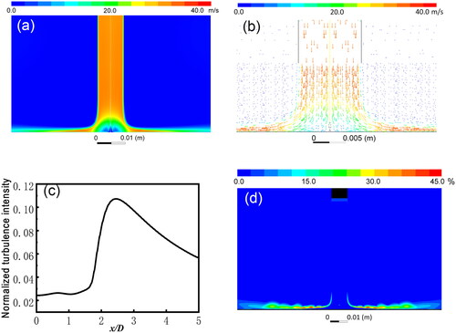
Turbophoresis is a possible reason for the second deposition peak. In the region near the second deposition peak, the turbulence intensity near the wall is lower than the turbulence intensity away from the wall, as the Figure 5d shows. Micro-droplets could drift from regions high turbulence intensity to regions with lower turbulence near the wall according to the turbophoresis theory. Caporaloni et al. (1975) proposed the turbophoresis theory and then Reeks (1983) reexamined later to explain the existence of the net discrete phase flux toward the wall. Marchioli and Soldati (2002) stated that in the case of ejection, particles are concentrated under the low-speed streaks and accumulate in the near-wall region with lower turbulence intensity. In the current simulation, the turbophoresis effect is calculated by the discrete random walk model.

Discussion

Necessity of two-way coupling

Two-way coupling considers the influence of the discrete phase on the flow field, which is more accurate but needs more computational resources. Different choices have been made in the literature. Anh Ho and Sommerfeld (2002) simulated the agglomeration in homogeneous isotropic turbulence with only one-way coupling. Elghobashi (1994) recommended two-way coupling when the discrete phase volume fraction, α_V, is greater than 10⁻⁶. Here we compare one-way and two-way results under different α_V, with coalescence being always considered. In the particle-laden flow simulation, two-way coupling method with inter-particle collision being considered is also referred to as four-way coupling (Elghobashi 1994).

The relative thickness is the subject to compare. In the simulation, the plate is divided into N concentric annuli. And m_i is the mass of droplets deposited on the annulus. As shown in Figure 6, the relative thickness τ at x/D = a is defined as τ_a = m_ai/m_total, where m_total is the total mass of droplets deposited on the plate and m_a is the total mass of droplets deposited on the annulus with diameter of aD. The average deviation $\Delta$ is defined to evaluate the difference between two pattern results (Bevington and Robinson 2003): (22) $$\Delta ={\left[\frac{1}{N}{\sum }_{i=1}^N({\tau }_i-{\tau }_{0i}{)}^2\right]}^{\frac{1}{2}}$$(22) where N is the number of the sample points, τ_i is the relative thickness at the sample point i and τ_0i is the relative thickness at the sample point i in two-way coupling method. In this study, $\Delta$ = 1% is set as the significance criterion for the average deviation.

Figure 6. Relative thickness distributions under different droplets volume fractions: (a) α_V = α_V0.1; (b) α_V = α_V1 = 10⁻⁵; (c) α_V = α_V2; (d) α_V = α_V4; (e) α_V = α_V8. The modeling choice of the one or two-way coupling with or without coalescence calculation are compared.

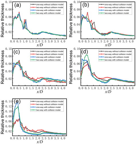
As shown in Figure 6, when the droplets volume fraction is small as α_V = α_V0.1, the patterns are almost the same, corresponding to $\Delta$ compared to two-way coupling with particle collision small as 0.36%. $\Delta$ is 0.32% and 0.34% for α_V1 and α_V2. $\Delta$ increases to 0.83% when α_V = α_V4, 0.5%. And for α_V8, $\Delta$ is 0.89% < 1%, suggesting that for the volume fraction smaller than 8 × 10⁻⁵, there is no need for two-way coupling method.

Necessity of coalescence calculation

As shown in Figure 6, we set the results using four-way coupling method as the accurate and evaluate the deviation when switching off the coalescence, i.e., collision. As illustrated, $\Delta$ is 0.25% when α_V = α_V0.1, indicating the coalescence model is not necessary. Then with greater fraction, $\Delta$ = 0.49%, when α_V = α_V2. And for α_V4 and α_V8, $\Delta$ are 0.96% and 1.78%. Therefore, α_V4 = 4.08 × 10⁻⁵ ≈ 4.0 × 10⁻⁵ can be treated as the criterion for the necessity of coalescence model. The results are consistent with the recommendation by Elghobashi (1994) that the critical volume fraction for micron particles coalescence varied from 10⁻⁵ to 10⁻³ and closer to 10⁻⁵ for smaller particles.

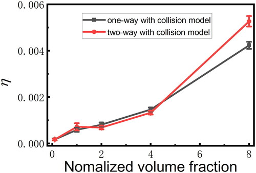
The coalescence does play an important role in the aerosol impingement by increasing the droplet size and reducing droplet number. The Sauter mean diameters (SMDs) of the deposited droplets are shown in Figure 7. Strömgren et al. (2012) found that the turbulence decreases with the increase of the particle volume fraction in two-way coupling method and the decrease of the turbulence can reduce the deposition of small droplets. The increase of SMD without coalescence in two-way coupling method can be explained by the decrease of small droplet ratio on the plate. The SMDs with coalescence are bigger than those without coalescence, and the difference is more significant with greater droplets volume fraction. The results agree qualitatively with the simulation results by Anh Ho and Sommerfeld (2002) that for monodisperse particles with the diameter of 5 µm, the collision frequency increased by around 7 times when α_V increased from 10⁻⁶ to 10⁻⁵. The collision ratio η is defined as: (23) $$\eta =\frac{n_c}{n_{\mathit{total}}}$$(23) where n_c is the number of particles that participate in collision and n_total is the total number of particles in the computational region within one time step. In the simulation, n_c and n_total are recorded in every time step. Figure 8 shows the average collision ratio η over 100 time steps during steady state. When the droplet volume fraction is as small as α_V0.1, collisions are rare. From α_V2 to α_V4, the collision ratio increases almost 2 times.

Figure 7. Results of the Sauter mean diameters of the deposited droplets under different simulation settings. The deposited droplets are bigger with the coalescence calculation.

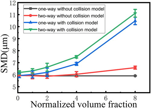
Figure 8. Simulated collision ratio with different droplet volume fractions.

As suggested above, the volume fraction of 8 × 10⁻⁵ can be the criterion for two-way coupling, while 4.0 × 10⁻⁵ can be the criterion for the necessity of coalescence calculation. Therefore, the collision and coalescences among the microdroplets could have more significant effect on the deposition pattern than the change of the flow field due to the dragging effect of the microdroplets. Note here the criterion is based on the result of deposition pattern rather than the flow field. The coalescences among the microdroplets change the size and number of the droplets and thus have direct impact on the deposition.

Conclusions

This work proposes a simulation scheme which considers the coalescence among the droplets and two-way coupling between the continuous and discrete phases. The simulation reproduces the concentric dual-ring deposition pattern observed in experiments of Liu et al. (2010). The inner ring is due to the inertia impact on the plate, and the outer ring is due to the droplet diffusion driven by the local turbulence intensity peak and turbophoresis. The necessity of coalescence calculation as well as two-way coupling is then analyzed. When the droplets volume fraction is less than 1 × 10⁻⁵, one-way coupling method without coalescence is accurate enough. When the droplets volume fraction exceeds 4 × 10⁻⁵, the coalescence would bring more than 1% difference in the deposition pattern. The influence of two-way coupling increases with the increase of discrete phase volume fraction and the influence is less than 1% for volume fraction smaller than 8 × 10⁻⁵ in the impinging jet.

Nomenclature
b, bcrit	=	collision parameter, critical collision parameter
Cc	=	Cunningham slip correction factor
c	=	number concentration of droplet
cpr	=	local droplet number density
D	=	inlet diameter of nozzle channel
dd	=	droplet diameter
f	=	elliptic relaxation function
H	=	height of the inject pipe
h	=	height of the jet nozzle above the solid plate
K	=	collision kernel
k	=	turbulent kinetic energy
kb	=	Boltzmann constant
L	=	length of the simulation region
l	=	length (diameter) of the solid plate
r1, r2	=	radius of droplets
Re	=	Reynolds number
T	=	temperature
t	=	time
$\overrightarrow{u}$	=	velocity of fluid
${\overrightarrow{u}}_d$	=	velocity of droplet
Vc, Vpr	=	mesh cell volume, physically reliable volume
vin	=	inlet jet velocity
$\overline{v^2}$	=	velocity variance scale
We	=	Weber number, $We= {\rho }_d{d}_d{\overline{u_d}}^2/\sigma$
x	=	the distance to the centerline in radial direction

Greek symbols
y+	=	non-dimensional distance in wall units
Y	=	random number between 0 and 1
z	=	the distance to the nozzle in streamwise direction
αV	=	volume fraction
ρ	=	fluid density
ρd	=	droplet density
δij	=	Kronecker delta
$\Delta$	=	statistical difference in different models
η	=	collision ratio
λ	=	molecular mean free path
µ	=	dynamic viscosity of the fluid
σ	=	surface tension of the droplet
ψ	=	number of droplet parcels in a cell

Subscripts
d	=	droplet
i	=	component of x coordinate
j	=	component of y coordinate

Additional information

Funding

This work was supported by National Key R&D Program of China, No. 2016YFB0600605 and National Natural Science Foundation of China, No. 51976001.

References

- Andersen, A. A. 1966. A sampler for respiratory health hazard assessment. Am. Ind. Hyg. Assoc. J. 27 (2):160–65. doi:https://doi.org/10.1080/00028896609342810.
- Andreassi, L., S. Ubertini, and L. Allocca. 2007. Experimental and numerical analysis of high pressure diesel spray–wall interaction. Int. J. Multiphase Flow 33 (7):742–65. doi:https://doi.org/10.1016/j.ijmultiphaseflow.2007.01.003.
- Angioletti, M., E. Nino, and G. Ruocco. 2005. CFD turbulent modelling of jet impingement and its validation by particle image velocimetry and mass transfer measurements. Int. J. Therm. Sci. 44 (4):349–56. doi:https://doi.org/10.1016/j.ijthermalsci.2004.11.010.
- Anh Ho, C., and M. Sommerfeld. 2002. Modelling of micro-particle agglomeration in turbulent flows. Chem. Eng. Sci. 57 (15):3073–84. doi:https://doi.org/10.1016/S0009-2509(02)00172-0.
- Arffman, A., M. Marjamäki, and J. Keskinen. 2011. Simulation of low pressure impactor collection efficiency curves. J. Aerosol Sci. 42 (5):329–40. doi:https://doi.org/10.1016/j.jaerosci.2011.02.006.
- Behnia, M., S. Parneix, and P. A. Durbin. 1998. Prediction of heat transfer in an axisymmetric turbulent jet impinging on a flat plate. Int. J. Heat Mass Transfer 41 (12):1845–55. doi:https://doi.org/10.1016/S0017-9310(97)00254-8.
- Behnia, M., S. Parneix, Y. Shabany, and P. A. Durbin. 1999. Numerical study of turbulent heat transfer in confined and unconfined impinging jets. Int. J. Heat Fluid Flow 20 (1):1–9. doi:https://doi.org/10.1016/S0142-727X(98)10040-1.
- Bevington, P. R., and D. K. Robinson. 2003. Data reduction and error analysis for the physical sciences. 3rd ed. New York: McGraw-Hill.
- Blomquist, G., G. Strom, and L. H. Stromquist. 1984. Sampling of high concentrations of airborne fungi. Scand. J. Work. Environ. Health 10 (2):109–13. doi:https://doi.org/10.5271/sjweh.2357.
- Caporaloni, M., F. Tampieri, F. Trombetti, and O. Vittori. 1975. Transfer of Particles in Nonisotropic Air Turbulence. J. Atmos. Sci. 32 (3):565–8. doi:https://doi.org/10.1175/1520-0469(1975)032<0565:TOPINA>2.0.CO;2.
- Chen, M., F. J. Romay, L. Li, A. Naqwi, and V. A. Marple. 2016. A novel quartz crystal cascade impactor for real-time aerosol mass distribution measurement. Aerosol Sci. Technol. 50 (9):971–83. doi:https://doi.org/10.1080/02786826.2016.1213790.
- Craft, T. J., L. J. W. Graham, and B. E. Launder. 1993. Impinging jet studies for turbulence model assessment—II. An examination of the performance of four turbulence models. Int. J. Heat Mass Transfer 36 (10):2685–97. doi:https://doi.org/10.1016/S0017-9310(05)80205-4.
- Durbin, P. A. 1993. A Reynolds stress model for near-wall turbulence. J. Fluid Mech. 249 (1):465–98. doi:https://doi.org/10.1017/S0022112093001259.
- Durbin, P. A. 2018. Some recent developments in turbulence closure modeling. Annu. Rev. Fluid Mech. 50 (1):77–103. doi:https://doi.org/10.1146/annurev-fluid-122316-045020.
- Elghobashi, S. 1994. On predicting particle-laden turbulent flows. Appl. Sci. Res. 52 (4):309–29. doi:https://doi.org/10.1007/BF00936835.
- Feng, J. Q. 2017. A computational study of particle deposition patterns from a circular laminar jet. J. Appl. Fluid Mech. 10 (4):1001–12. doi:https://doi.org/10.18869/acadpub.jafm.73.241.27233.
- Feng, J. Q. 2018. Mist flow visualization for round jets in Aerosol Jet® printing. Aerosol Sci. Technol. 51 (3):1–8. doi:https://doi.org/10.1080/02786826.2018.1532566.
- Feng, J. Q., and M. J. Renn. 2019. Aerosol Jet® direct-write for microscale additive manufacturing. J. Micro Nano Manuf. 7 (1):011004. doi:https://doi.org/10.1115/1.4043595.
- Fénot, M., X. T. Trinh, and E. Dorignac. 2019. Flow and heat transfer of a compressible impinging jet. Int. J. Therm. Sci. 136:357–69. doi:https://doi.org/10.1016/j.ijthermalsci.2018.10.035.
- Ghadimi, P., M. Yousefifard, and H. Nowruzi. 2017. Particle and gas flow modeling of wall-impinging diesel spray under ultra-high fuel injection pressures. J. Appl. Fluid Mech. 10 (5):1283–91. doi:https://doi.org/10.18869/acadpub.jafm.73.242.27259.
- Gosman, A. D., and E. Loannides. 1983. Aspects of computer simulation of liquid-fueled combustors. Energy. J. 7 (6):482–90. doi:https://doi.org/10.2514/3.62687.
- Jambunathan, K., E. Lai, M. A. Moss, and B. L. Button. 1992. A review of heat transfer data for single circular jet impingement. Int. J. Heat Fluid Flow 13 (2):106–15. doi:https://doi.org/10.1016/0142-727X(92)90017-4.
- Jaramillo, J. E., F. X. Trias, A. Gorobets, C. D. Prez-Segarra, and A. Oliva. 2012. DNS and RANS modelling of a turbulent plane impinging jet. Int. J. Heat Mass Transfer 55 (4):789–801. doi:https://doi.org/10.1016/j.ijheatmasstransfer.2011.10.031.
- Jones, C. S., X. Lu, M. Renn, M. Stroder, and W.-S. Shih. 2010. Aerosol-jet-printed, high-speed, flexible thin-film transistor made using single-walled carbon nanotube solution. Microelectron. Eng. 87 (3):434–7. doi:https://doi.org/10.1016/j.mee.2009.05.034.
- Li, Q., T-m Cai, G-q He, and C-b Hu. 2006. Droplet collision and coalescence model. Appl. Math. Mech. 27 (1):67–73.
- Li, W., J. Ren, J. Hongde, and P. Ligrani. 2016. Assessment of six turbulence models for modeling and predicting narrow passage flows, part 1: Impingement jets. Numer. Heat Transf. Part A Appl. 69 (2):109–27. doi:https://doi.org/10.1080/10407782.2015.1069665.
- Litchford, R. J., and S.-M. Jeng. 1991. Efficient statistical transport model for turbulent particle dispersion in sprays. AIAA J. 29 (9):1443–51. doi:https://doi.org/10.2514/3.59965.
- Liu, T., J. Nink, P. Merati, T. Tian, Y. Li, and T. Shieh. 2010. Deposition of micron liquid droplets on wall in impinging turbulent air jet. Exp. Fluids 48 (6):1037–57. doi:https://doi.org/10.1007/s00348-009-0790-7.
- Marchioli, C., and A. Soldati. 2002. Mechanisms for particle transfer and segregation in a turbulent boundary layer. J. Fluid Mech. 468:283–315. doi:https://doi.org/10.1017/S0022112002001738.
- Marple, V., B. Olson, F. Romay, G. Hudak, S. M. Geerts, and D. Lundgren. 2014. Second generation micro-orifice uniform deposit impactor, 120 MOUDI-II: Design, evaluation, and application to long-term ambient sampling. Aerosol Sci. Technol. 48 (4):427–33. doi:https://doi.org/10.1080/02786826.2014.884274.
- Marple, V., K. Rubow, G. Ananth, and H. J. Fissan. 1986. Micro-orifice uniform deposit impactor. J. Aerosol Sci. 17 (3):489–94. doi:https://doi.org/10.1016/0021-8502(86)90141-2.
- Mette, A., P. L. Richter, M. Hörteis, and S. W. Glunz. 2007. Metal aerosol jet printing for solar cell metallization. Prog. Photovolt Res. Appl. 15 (7):621–7. doi:https://doi.org/10.1002/pip.759.
- Meyer, C. J., and D. A. Deglon. 2011. Particle collision modeling—A review. Miner. Eng. 24 (8):719–30. doi:https://doi.org/10.1016/j.mineng.2011.03.015.
- Morsi, S. A., and A. J. Alexander. 1972. An investigation of particle trajectories in two-phase flow systems. J. Fluid Mech. 55 (02):193–208. doi:https://doi.org/10.1017/S0022112072001806.
- Mottaghi, P., M. Abbasalizadeh, and H. Ahmady-Birgani. 2019. Depositional arrangement of non-spherical atmospheric particles on impaction plate of a multi-nozzle impactor. Aerosol Sci. Technol. 53 (12):1381–92.
- Mundo, C., M. Sommerfeld, and C. Tropea. 1995. Droplet-wall collisions: Experimental studies of the deformation and breakup process. Int. J. Multiphase Flow 21 (2):151–73. doi:https://doi.org/10.1016/0301-9322(94)00069-V.
- O’Rourke, P. J. 1981. Collective Drop Effects on Vaporizing Liquid Sprays. Princeton, NJ: Princeton University.
- Oesterle, B., and A. Petitjean. 1993. Simulation of particle-to-particle interactions in gas solid flows. Int. J. Multiphase Flow 19 (1):199–211. doi:https://doi.org/10.1016/0301-9322(93)90033-Q.
- Otto, E., H. Fissan, S. H. Park, and K. W. Lee. 1999. The log-normal size distribution theory of brownian aerosol coagulation for the entire particle size range: Part II—Analytical solution using Dahneke’s coagulation kernel. J. Aerosol Sci. 30 (1):17–34. doi:https://doi.org/10.1016/S0021-8502(98)00038-X.
- Ounis, H., G. Ahmadi, and J. B. McLaughlin. 1991. Brownian diffusion of submicrometer particles in the viscous sublayer. J. Colloid Interface Sci. 143 (1):266–77. doi:https://doi.org/10.1016/0021-9797(91)90458-K.
- Reeks, M. W. 1983. The transport of discrete particles in inhomogeneous turbulence. J. Aerosol Sci. 14 (6):729–39. doi:https://doi.org/10.1016/0021-8502(83)90055-1.
- Saffman, P. G., and J. S. Turner. 1956. On the collision of drops in turbulent clouds. J. Fluid Mech. 1 (01):16–30. doi:https://doi.org/10.1017/S0022112056000020.
- Satake, S. i., and T. Kunugi. 1998. Direct numerical simulation of an impinging jet into parallel disks. Int. J. Num. Meth. HFF. 8 (7):768–80. doi:https://doi.org/10.1108/09615539810232871.
- Schmidt, D. P., and C. J. Rutland. 2000. A new droplet collision algorithm. Comput. Phys. 164 (1):62–80. doi:https://doi.org/10.1006/jcph.2000.6568.
- Šikalo, Š., C. Tropea, and E. N. Ganić. 2005. Impact of droplets onto inclined surfaces. J. Colloid Interface Sci. 286 (2):661–9. doi:https://doi.org/10.1016/j.jcis.2005.01.050.
- Sommerfeld, M. 2001. Validation of a stochastic Lagrangian modelling approach for inter-particle collisions in homogeneous isotropic turbulence. Int. J. Multiphase Flow 27 (10):1829–58. doi:https://doi.org/10.1016/S0301-9322(01)00035-0.
- Strömgren, T., G. Brethouwer, G. Amberg, and A. V. Johansson. 2012. Modelling of turbulent gas-particle flows with focus on two-way coupling effects on turbophoresis. Powder Technol. 224:36–45. doi:https://doi.org/10.1016/j.powtec.2012.02.017.
- Tait, J. G., E. Witkowska, M. Hirade, T.-H. Ke, P. E. Malinowski, S. Steudel, C. Adachi, and P. Heremans. 2015. Uniform Aerosol Jet printed polymer lines with 30µm width for 140ppi resolution RGB organic light emitting diodes. Org. Electron. 22:40–3. doi:https://doi.org/10.1016/j.orgel.2015.03.034.
- Tian, L., and G. Ahmadi. 2007. Particle deposition in turbulent duct flows—Comparisons of different model predictions. J. Aerosol Sci. 38 (4):377–97. doi:https://doi.org/10.1016/j.jaerosci.2006.12.003.
- Wang, C., S. Chang, M. Leng, H. Wu, and B. Yang. 2016. A two-dimensional splashing model for investigating impingement characteristics of supercooled large droplets. Int. J. Multiphase Flow 80:131–49. doi:https://doi.org/10.1016/j.ijmultiphaseflow.2015.12.005.
- Wang, L.-P., A. S. Wexler, and Y. Zhou. 1998. Statistical mechanical descriptions of turbulent coagulation. Phys. Fluids 10 (10):2647–51.
- Wang, L.-P., A. S. Wexler, and Y. Zhou. 2000. Statistical mechanical description and modelling of turbulent collision of inertial particles. J. Fluid Mech. 415:117–53. doi:https://doi.org/10.1017/S0022112000008661.
- Wierzba, A. 1990. Deformation and breakup of liquid drops in a gas stream at nearly critical Weber numbers. Exp. Fluids 9 (1-2):59–64. doi:https://doi.org/10.1007/BF00575336.
- Wu, J., J. Xu, and H. Wang. 2018. Numerical simulation of micron and submicron droplets in jet impinging. Adv. Mech. Eng. 10 (10):168781401880531. doi:https://doi.org/10.1177/1687814018805319.
- Xu, J., H. Shen, and H. Wang. 2015. An industry-scale modeling for the turbulence agglomeration of fine particles. Adv. Mech. Eng. 7 (11):168781401561767. doi:https://doi.org/10.1177/1687814015617670.
- Zaichik, L. I., and A. L. Solov’ev. 2002. Collision and coagulation nuclei under conditions of brownian and turbulent motion of aerosol particles. High Temp. 40 (3):422–7.
- Zhang, J., J. Mi, and H. Wang. 2012. A new mesh-independent model for droplet/particle collision. Aerosol Sci. Technol. 46 (6):622–30. doi:https://doi.org/10.1080/02786826.2011.649809.
- Zhang, Z., P. X. Jiang, X. L. Ouyang, J. N. Chen, and D. M. Christopher. 2014. Experimental investigation of spray cooling on smooth and micro-structured surfaces. Int. J. Heat Mass Transfer 76:366–75. doi:https://doi.org/10.1016/j.ijheatmasstransfer.2014.04.010.
- Zhao, D., T. Liu, J. G. Park, M. Zhang, J.-M. Chen, and B. Wang. 2012. Conductivity enhancement of aerosol-jet printed electronics by using silver nanoparticles ink with carbon nanotubes. Microelectron. Eng 96:71–5. doi:https://doi.org/10.1016/j.mee.2012.03.004.
- Zhou, T., D. Xu, J. Chen, C. Cao, and T. Ye. 2016. Numerical analysis of turbulent round jet impingement heat transfer at high temperature difference. Appl. Therm. Eng. 100:55–61. doi:https://doi.org/10.1016/j.applthermaleng.2016.02.006.
- Zhou, Y., A. S. Wexler, and L.-P. Wang. 2001. Modelling turbulent collision of bidisperse inertial particles. J. Fluid Mech. 433:77–104. doi:https://doi.org/10.1017/S0022112000003372.
- Zuckerman, N., and N. Lior. 2006. Jet impingement heat transfer: Physics, correlations, and numerical modeling. Advances in heat transfer 39:565–631. doi:https://doi.org/10.1016/S0065-2717(06)39006-5.