Distribution and penetration efficiency of cylindrical nanoparticles in turbulent flows through a curved tube

Abstract

Distribution and penetration efficiency of cylindrical nanoparticles with length of 160 nm and aspect ratio between 2 and 16 are studied numerically in turbulent flows through a curved tube in the range of Reynolds number from 4500 to 43,000, Stokes number from 0.002 to 0.026, Dean number from 1428 to 2884. The distributions of particle number concentration and particle orientation on the cross-section at different axial positions and outlet are given and analyzed. The effect of various parameters on the penetration efficiency is discussed. The results showed that the extent of non-uniformity of the distribution of particle number concentration increases with increasing Stokes number, Dean number, Reynolds number and particle aspect ratio. More particles align with their major axis near to the flow direction with the increase of the Stokes number and particle aspect ratio, than with the decrease of the Dean number and Reynolds number. The penetration efficiency increases as the Dean number, Reynolds number and particle aspect ratio decrease. However, the penetration efficiency is not a monotonic function of the Stokes number. The penetration efficiency increases and decreases with the increasing Stokes number when St < 0.02 and St > 0.02, respectively. Finally, the relationship between the penetration efficiency and related synthetic parameters is established based on the numerical data.

Copyright © 2020 American Association for Aerosol Research

EDITOR:

• Yannis Drossinos

1. Introduction

Conveying of aerosol particles by flowing air through tubes under turbulent flow conditions is very common in a wide range of practical applications such as air ventilation systems, pneumatic conveyers, human respiratory system and so on. In the conveying process, aerosol particle deposition in tubes may block flow, cause malfunction and reduce system efficiency, or affect people’s health. This shows that the research on conveying and deposition of aerosol particles in tubes is significant for engineering applications. In the past years, there have been many related researches addressing the conveying and deposition of aerosol particles in straight tubes (e.g., Anand et al. 1992; Shapiro and Goldenberg 1993; Muyshondt, Anand, and McFarland 1996; Armand et al. 1998; Lin, Zhang, and Zhang 2006; Phares and Sharma 2006; Lin, Qian et al. 2009; Lin et al. 2014; Matsusaka 2015). However, curved tubes are frequently used in practical applications. The fluid in curved tubes experiences a centrifugal force which results in secondary flow and transports particles toward the walls, greatly changing particle distribution and deposition downstream of the tube. Therefore, it is important to explore the particle distribution, deposition and penetration efficiency in the turbulent flows through a curved tube. There have been many researches on this issue. However, many investigations were focused on the microsized or larger particles (e.g., Tsai and Pui 1990; Peters and Leith 2004; Quek, Wang, and Ray 2005; Sun et al. 2013).

Actually nanosized aerosol particles are very common in the application. The effects of flow property and tube curvature on the motion, distribution and deposition of nanosized particles are different from those of microsized or larger particles. Pui, Romay-Novas, and Liu (1987) studied experimentally the penetration efficiency of particles with diameters of 0.1 μm ≤ d_p ≤ 10 μm and Reynolds numbers of 100 < Re < 10,000, and showed that the penetration efficiency did not depend on either the curvature or the Reynolds number. Balásházy, Martonen, and Hofmann (1990) studied the inertial impaction and gravitational deposition of aerosols, and found that the deposition efficiency was not strongly affected by secondary flow in airway cross-sections for the case of inhalation. Lee and Giesekej (1994) showed that, for aerosols with diameter of 0.035–1.3 μm and Reynolds numbers of 1800–15,600, the previous theories alone did not predict satisfactorily the deposition rates in the regime closer to minimum deposition when both inertial deposition and Brownian diffusional mechanisms operated simultaneously. Sato, Chen, and Pui (2003) found that the deposition efficiency of particles was enhanced with the increase of the Stokes number and Dean number, and with the decrease of the curvature ratio. Wang, Flagan, and Seinfeld (2002) found that the increase in the diffusion losses of particle with diameter of 5–15 nm due to bends was sensitive to both the bends orientations and the lengths of straight tubing between them when Reynolds number is low. Yook and Pui (2006) found that the penetration efficiency of particle with diameter of 3–50 nm increased with the increase of particle size and Dean number in the range of De = 21–1779, while the effect of curvature ratio on the penetration efficiency seemed to be negligible when De > 200. Lin, Lin et al. (2009) showed that the nanoparticle distributions were mostly determined by the axial velocity when the Schmidt number is small, while the secondary flow would dominate the nanoparticle distribution when the Schmidt number is many orders of magnitude larger than 1. Particle deposition became uniform with increasing Dean number. Wilson et al. (2011) showed that increased Reynolds number did not greatly change the trend of deposition fraction with a certain Stokes number range. However, a significant increase in deposition was observed for 0.1 ≤ St ≤ 0.4. An increase in Reynolds number from 10,250 to 30,750 resulted in a factor of 2.6 increase in deposition fraction from 0.14 to 0.36 at St = 0.15. Ghaffarpasand et al. (2012) found that the penetration efficiency of particle with diameter of 3–17 nm increased with the increase of the curvature ratios in the range of De = 1426–2885, while was insensitive to the Reynolds number. Lin et al. (2015) showed that the effect of Dean number on the penetration efficiency of particles with diameter of 8–550 nm was dependent on the Schmidt number. There existed a critical Dean number beyond which the penetration efficiency turned from increment to decrement, and this critical value was dependent on the Schmidt number. The penetration efficiencies are higher in the case of higher Dean number than that of lower one.

As aforementioned, the studies have been focused on the spherical particles. However, the conveying of non-spherical particles, e.g., cylindrical or ellipsoidal particles is also very common. The migration of non-spherical aerosol particles in the flow is quite complicated because particle rotation and its orientation are strongly coupled with the translation motion. However, there is a lack of study on the transport, distribution and penetration efficiency of non-spherical particles in turbulent flows through a curved tube. Such case can be found in the actual situation, e.g., airway bifurcations in human respiratory system. Cylindrical particle is one of the most common particles among the non-spherical particles. Therefore, in the present study, the equations of mean momentum, turbulent kinetic energy and dissipation rate, and fluctuating velocity of fluid are solved first, and then the equations of cylindrical particle motion and orientation are solved to obtain the distributions of particle number concentration and particle orientation on the cross-section for different parameters. Finally, the penetration efficiency is calculated and the relationship between it and related synthetic parameters is built up based on the numerical data.

2. Flow field and coordinate systems

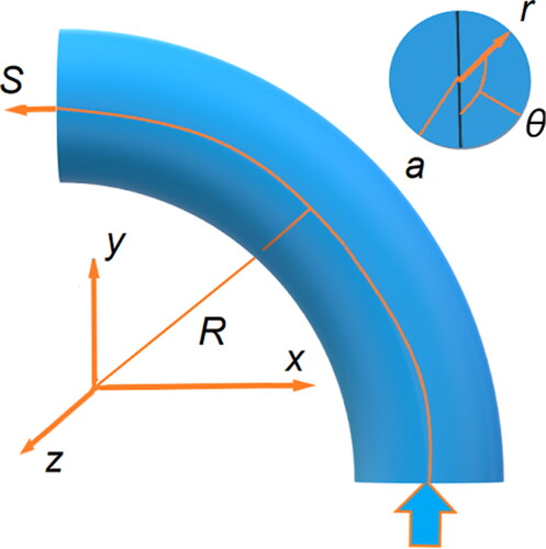
Cylindrical particulate flow through a curved tube and the coordinate system are shown in Figure 1 where centerline S of the tube is located in the x–y plane, and r and θ are the polar coordinates defined in the cross-section. u, v and w are the velocity components in the directions of r, θ and S, respectively. a and R are the tube inner radius and curved radius, respectively.

Figure 1. Cylindrical particulate flow through a curved tube.

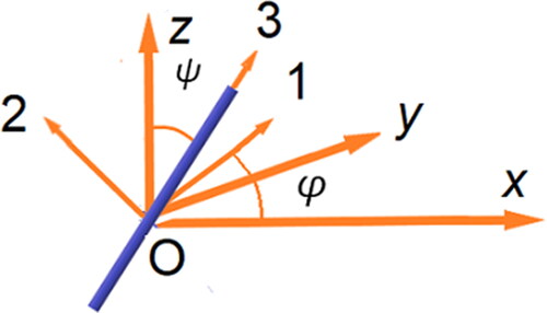
Orientation of a cylindrical particle in the fixed coordinate system-xyz can be determined by φ and ψ as shown in Figure 2 where the coordinate system-123 is fixed in the particle, direction 3 is along the particle long axis, 1 is the direction of projection of particle long axis on the x–y plane, 2 is the direction perpendicular to the 1–3 plane, φ is the angle between the projection of particle on the x–y plane and the x-axis. The transform matrix from coordinate system-xyz to coordinate system-123 is: (1) $$A={\left|\begin{array}{ccc}\text{cos}\psi \text{cos}\phi & \text{cos}\psi \text{sin}\phi & -\text{sin}\psi \\ -\text{sin}\phi & \text{cos}\phi & 0\\ \text{sin}\psi \text{cos}\phi & \text{sin}\psi \text{sin}\phi & \text{cos}\psi \end{array}\right|}^T=\left|\begin{array}{c}{a}_{11}\mathrm{ }{a}_{12}\mathrm{ }{a}_{13}\\ a_{21}\mathrm{ }{a}_{22}\mathrm{ }{a}_{23}\\ a_{31}\mathrm{ }{a}_{32}\mathrm{ }{a}_{33}\end{array}\right|,$$(1) and the unit vector p along the principal axis of the particle is (2) $$\mathit{p}={\left[\begin{array}{ccc}{a}_{31}& a_{32}& a_{33}\end{array}\right]}^T.$$(2)

Figure 2. Two coordinate systems.

Due to a possible singularity in the inversion of the transformation matrix the quaternions (ε₁, ε₂, ε₃, η) are used (3) $$A=\left|\begin{array}{ccc}1-2\left({\epsilon }_2^2+{\epsilon }_3^2\right)& 2\left({\epsilon }_1{\epsilon }_2+{\epsilon }_3\eta \right)& 2\left({\epsilon }_1{\epsilon }_3-{\epsilon }_2\eta \right)\\ 2\left({\epsilon }_1{\epsilon }_2-{\epsilon }_3\eta \right)& 1-2\left({\epsilon }_3^2+{\epsilon }_1^2\right)& 2\left({\epsilon }_2{\epsilon }_3+{\epsilon }_1\eta \right)\\ 2\left({\epsilon }_1{\epsilon }_3+{\epsilon }_2\eta \right)& 2\left({\epsilon }_2{\epsilon }_3-{\epsilon }_1\eta \right)& 1-2\left({\epsilon }_1^2+{\epsilon }_2^2\right)\end{array}\right|.$$(3)

The quaternions are related to the Euler angles as (4) $$\left|\begin{array}{c}{\epsilon }_1\\ {\epsilon }_2\\ {\epsilon }_3\end{array}\right|=\frac{1}{4\eta }|\begin{array}{c}{a}_{23}-a_{32}\\ a_{31}-a_{13}\\ a_{12}-a_{21}\end{array}|=\frac{1}{4\eta }|\begin{array}{c}-\text{sin}\psi \text{sin}\phi \\ \text{sin}\psi \left(\text{cos}\phi +1\right)\\ \text{sin}\phi \left(\text{cos}\psi +1\right)\end{array}|,\mathrm{ }\eta =\sqrt{1+a_{11}+a_{22}+a_{33}},$$(4) (5) $${\epsilon }_1=\sqrt{\frac{1+a_{11}}{2}},\mathrm{ }{\epsilon }_2=\frac{a_{12}}{2{\epsilon }_1},\mathrm{ }{\epsilon }_3=\frac{a_{23}}{2{\epsilon }_2},\mathrm{ }\text{when}\mathrm{ }\eta \mathrm{ }=\mathrm{ }0.$$(5)

The particle angular velocity can be represented in the particle frame as (6) $$\left|\begin{array}{c}\frac{d\eta }{dt}\\ \frac{d{\epsilon }_1}{dt}\\ \frac{d{\epsilon }_2}{dt}\\ \frac{d{\epsilon }_3}{dt}\end{array}\right|=\frac{1}{2}|\begin{array}{c}-{\epsilon }_1{\omega }_1-{\epsilon }_2{\omega }_2-{\epsilon }_3{\omega }_3\\ \eta {\omega }_1-{\epsilon }_3{\omega }_2+{\epsilon }_2{\omega }_3\\ {\epsilon }_3{\omega }_1+\eta {\omega }_2-{\epsilon }_1{\omega }_3\\ -{\epsilon }_2{\omega }_1+{\epsilon }_1{\omega }_2+\eta {\omega }_3\end{array}|,\mathrm{ }$$(6) where ω₁, ω₂ and ω₃ are the three components of angular velocity in the particle frame.

3. Governing equations

3.1. Cylindrical particle

The particles in the present study are rigid cylindrical particles. According to the general assumptions, the flow around a particle is the Stokes flow of a Newtonian fluid, and the effect of particles on the suspending fluid is negligible.

3.1.1. Slender-body theory

The motion of cylindrical particle is modeled based on the slender-body theory (Batchelor 1970), i.e., the disturbance motion induced by the cylindrical particle is approximately the same as that induced by a line distribution of Stokeslets. A Stokeslet is a singularity in the Stokes flow and represents the effect of a force applied to the fluid at a point. In the slender-body theory, the cylinder is divided into several segments and the force exerted on a segment is represented by a point force. Although the force acting on a point is isotropic, the force acting on the whole cylinder is non-isotropic.

Based on the solution of the Stokes equation, the induced velocity of a point force exerted on the fluid is given by (7) $$V\left(x\right)=\mathit{F}\cdot \frac{G\left(x\right)}{8\pi \mu },{\mathit{G}}_{ij}=\frac{1}{r}{\delta }_{ij}+\frac{1}{r^3}{x}_i{x}_j,$$(7) where F is the force exerted on a cylindrical particle; G is a Green tensor. Integrating along the particle and simplifying the expression with the slender body approximation, the induced velocity can be obtained (Mackaplow and Shaqfeh 1998) as (8) $$\mathit{u}({\mathit{x}}_{\mathrm{c}}+ls\mathit{p})-[{\mathit{v}}_{\mathrm{p}}+(\mathit{\omega }\times ls\mathit{p}\left)\right]=-2\left(\ln 2\beta +\ln \frac{\sqrt{1-s^2}}{b\left(s\right)}\right)(\mathit{\delta }+\mathit{pp})\cdot \mathit{f}\left(s\right)-(\mathit{\delta }-3\mathit{p}\mathit{p})\cdot \mathit{f}\left(s\right)-(\mathit{\delta }+\mathit{pp})\cdot \int \frac{\mathit{f}\left(s\right)-\mathit{f}\left(s^{\mathrm{\prime }}\right)}{\left|s-s^{\mathrm{\prime }}\right|}d{s}^{\mathrm{\prime }},$$(8) where u is the instantaneous velocity of the fluid; x_c is the coordinate of the particle mass center; v_p and ω are the particle velocity and angular velocity, respectively; p and l are the unit orientation vector and length of the particle, respectively; s is the dimensionless coordinate along the particle axis with –1 ≤ s ≤ 1; β is the particle aspect ratio; b(s) is the shape factor of the cross-section at$s$ (b(s) = 1 for cylindrical particle); δ is the unit matrix; f(s) is the force exerted on the particle by fluid and is an unknown variable. The terms on the left-hand side of Equation (8)(8) $$\mathit{u}({\mathit{x}}_{\mathrm{c}}+ls\mathit{p})-[{\mathit{v}}_{\mathrm{p}}+(\mathit{\omega }\times ls\mathit{p}\left)\right]=-2\left(\ln 2\beta +\ln \frac{\sqrt{1-s^2}}{b\left(s\right)}\right)(\mathit{\delta }+\mathit{pp})\cdot \mathit{f}\left(s\right)-(\mathit{\delta }-3\mathit{p}\mathit{p})\cdot \mathit{f}\left(s\right)-(\mathit{\delta }+\mathit{pp})\cdot \int \frac{\mathit{f}\left(s\right)-\mathit{f}\left(s^{\mathrm{\prime }}\right)}{\left|s-s^{\mathrm{\prime }}\right|}d{s}^{\mathrm{\prime }},$$(8) are the velocity difference between the particle and the fluid at a point. The particle is first divided into M segments according to the Gauss integral point, and then f(s) is transformed to f(s_i) on each segment, finally the integration of the right-hand side of Equation (8)(8) $$\mathit{u}({\mathit{x}}_{\mathrm{c}}+ls\mathit{p})-[{\mathit{v}}_{\mathrm{p}}+(\mathit{\omega }\times ls\mathit{p}\left)\right]=-2\left(\ln 2\beta +\ln \frac{\sqrt{1-s^2}}{b\left(s\right)}\right)(\mathit{\delta }+\mathit{pp})\cdot \mathit{f}\left(s\right)-(\mathit{\delta }-3\mathit{p}\mathit{p})\cdot \mathit{f}\left(s\right)-(\mathit{\delta }+\mathit{pp})\cdot \int \frac{\mathit{f}\left(s\right)-\mathit{f}\left(s^{\mathrm{\prime }}\right)}{\left|s-s^{\mathrm{\prime }}\right|}d{s}^{\mathrm{\prime }},$$(8) is transformed to a linear summation of a series of f(s_i). Thus, Equation (8)(8) $$\mathit{u}({\mathit{x}}_{\mathrm{c}}+ls\mathit{p})-[{\mathit{v}}_{\mathrm{p}}+(\mathit{\omega }\times ls\mathit{p}\left)\right]=-2\left(\ln 2\beta +\ln \frac{\sqrt{1-s^2}}{b\left(s\right)}\right)(\mathit{\delta }+\mathit{pp})\cdot \mathit{f}\left(s\right)-(\mathit{\delta }-3\mathit{p}\mathit{p})\cdot \mathit{f}\left(s\right)-(\mathit{\delta }+\mathit{pp})\cdot \int \frac{\mathit{f}\left(s\right)-\mathit{f}\left(s^{\mathrm{\prime }}\right)}{\left|s-s^{\mathrm{\prime }}\right|}d{s}^{\mathrm{\prime }},$$(8) is transformed into 3M linear equations: (9) $$\mathit{u}({\mathit{x}}_{\mathrm{c}}+l{s}_i\mathit{p})-[{\mathit{v}}_{\mathrm{p}}+(\mathit{\omega }\times l{s}_i\mathit{p}\left)\right]=-\left[2\right(\ln 2\beta +\ln \sqrt{1-s_i^2}\left)\right(\mathit{\delta }+\mathit{pp})+(\mathit{\delta }-3\mathit{p}\mathit{p}\left)\right]\cdot \mathit{f}\left(s_i\right)+{\sum }_{\begin{array}{c}m=1\\ m\ne i\end{array}}^M\frac{l_m}{\left|s_i-s_m\right|}(\mathit{\delta }+\mathit{pp})\cdot \mathit{f}\left(s_i\right)-{\sum }_{\begin{array}{c}m=1\\ m\ne i\end{array}}^M{k}_{im}=\frac{l_m}{\left|s_i-s_m\right|}(\mathit{\delta }+\mathit{pp})\cdot \mathit{f}\left(s_m\right)\hspace{1em}(i=1,2,\dots ,M),$$(9) where l_m is the mth segment of the particle. f(s_i) is obtained by solving Equation (9)(9) $$\mathit{u}({\mathit{x}}_{\mathrm{c}}+l{s}_i\mathit{p})-[{\mathit{v}}_{\mathrm{p}}+(\mathit{\omega }\times l{s}_i\mathit{p}\left)\right]=-\left[2\right(\ln 2\beta +\ln \sqrt{1-s_i^2}\left)\right(\mathit{\delta }+\mathit{pp})+(\mathit{\delta }-3\mathit{p}\mathit{p}\left)\right]\cdot \mathit{f}\left(s_i\right)+{\sum }_{\begin{array}{c}m=1\\ m\ne i\end{array}}^M\frac{l_m}{\left|s_i-s_m\right|}(\mathit{\delta }+\mathit{pp})\cdot \mathit{f}\left(s_i\right)-{\sum }_{\begin{array}{c}m=1\\ m\ne i\end{array}}^M{k}_{im}=\frac{l_m}{\left|s_i-s_m\right|}(\mathit{\delta }+\mathit{pp})\cdot \mathit{f}\left(s_m\right)\hspace{1em}(i=1,2,\dots ,M),$$(9) , then the total force and toque exerted on the cylindrical particle by the fluid are obtained through solving following equation using numerical integration: (10) $$F=8\pi \mu l{\int }_{-1}^{1}f\left(s\right)ds, L=8\pi \mu l^2{\int }_{-1}^{1}sp\times f\left(s\right)ds.$$(10)

3.1.2. Equations of particle motion

The motion equations of a cylindrical particle under the effect of drag force, centrifugal force and random force are (based on the Stokes–Einstein dispersion) (Michaelides 2015) given by (11) $$m\frac{d{v}_{\mathrm{p}}}{dt}=\frac{F}{C_c}+m\frac{v_{\mathrm{p}S}^2}{(R+r)}+{\mathit{R}}_{\mathrm{b}}\sqrt{\frac{6\pi d_{\mathrm{pe}}{k}_{B}T\mu }{\mathrm{\Delta }t}},$$(11) (12) $$J_1\frac{d{\omega }_1}{dt}+\left(J_3-J_2\right){\omega }_2{\omega }_3=\frac{L_1}{C_{\mathrm{c}}},\mathrm{ }{J}_2\frac{d{\omega }_2}{dt}+\left(J_1-J_3\right){\omega }_3{\omega }_1=\frac{L_2}{C_{\mathrm{c}}},\mathrm{ }{J}_3\frac{d{\omega }_3}{dt}+\left(J_2-J_1\right){\omega }_1{\omega }_2=\frac{L_3}{C_{\mathrm{c}}}$$(12) (13) $$C_{\mathrm{c}}=1+2.257\left(\frac{2\lambda }{d_{\mathrm{pe}}}\right)+0.4\left(\frac{2\lambda }{d_{\mathrm{pe}}}\right)\exp (\frac{\mathrm{–}0.55d_{\mathrm{pe}}}{\lambda }),$$(13) where m is the particle mass; R_b is a random vector of Gaussian random components with zero mean and unit variance; d_pe is the volume-equivalent diameter of cylindrical particle; k_B is the Boltzmann constant; T is the temperature; μ is the dynamic viscosity of fluid; Δt is the time interval of action of the random force; J_i is the moment of inertia of particle; L_i is the component of torque; ω_i is the component of particle angular velocity; subscript 1, 2 and 3 represents three components in the coordinate system-123; C_c is the Cunningham slip correction factor; λ is the mean free path of the gas molecules. The Cunningham slip correction represents a correction to Stokes’ drag and the friction between particles and fluids due to the breakdown of the continuum assumption for very small particles. In Equation (11)(11) $$m\frac{d{v}_{\mathrm{p}}}{dt}=\frac{F}{C_c}+m\frac{v_{\mathrm{p}S}^2}{(R+r)}+{\mathit{R}}_{\mathrm{b}}\sqrt{\frac{6\pi d_{\mathrm{pe}}{k}_{B}T\mu }{\mathrm{\Delta }t}},$$(11) , the translational motion of particles is caused by the Stokes’ drag. In Equation (12)(12) $$J_1\frac{d{\omega }_1}{dt}+\left(J_3-J_2\right){\omega }_2{\omega }_3=\frac{L_1}{C_{\mathrm{c}}},\mathrm{ }{J}_2\frac{d{\omega }_2}{dt}+\left(J_1-J_3\right){\omega }_3{\omega }_1=\frac{L_2}{C_{\mathrm{c}}},\mathrm{ }{J}_3\frac{d{\omega }_3}{dt}+\left(J_2-J_1\right){\omega }_1{\omega }_2=\frac{L_3}{C_{\mathrm{c}}}$$(12) , the Cunningham slip correction for particle rotation should be different from that for particle translational motion. Here, before finding a suitable C_c for particle rotation, we assume that the particle rotation is caused by the toque which equals to Stokes’ drag multiplying an arm of force. Therefore, the Cunningham slip correction is used in Equations (11)(11) $$m\frac{d{v}_{\mathrm{p}}}{dt}=\frac{F}{C_c}+m\frac{v_{\mathrm{p}S}^2}{(R+r)}+{\mathit{R}}_{\mathrm{b}}\sqrt{\frac{6\pi d_{\mathrm{pe}}{k}_{B}T\mu }{\mathrm{\Delta }t}},$$(11) and (12)(12) $$J_1\frac{d{\omega }_1}{dt}+\left(J_3-J_2\right){\omega }_2{\omega }_3=\frac{L_1}{C_{\mathrm{c}}},\mathrm{ }{J}_2\frac{d{\omega }_2}{dt}+\left(J_1-J_3\right){\omega }_3{\omega }_1=\frac{L_2}{C_{\mathrm{c}}},\mathrm{ }{J}_3\frac{d{\omega }_3}{dt}+\left(J_2-J_1\right){\omega }_1{\omega }_2=\frac{L_3}{C_{\mathrm{c}}}$$(12) . The Cunningham slip correction factor is not included in the random force in Equation (11)(11) $$m\frac{d{v}_{\mathrm{p}}}{dt}=\frac{F}{C_c}+m\frac{v_{\mathrm{p}S}^2}{(R+r)}+{\mathit{R}}_{\mathrm{b}}\sqrt{\frac{6\pi d_{\mathrm{pe}}{k}_{B}T\mu }{\mathrm{\Delta }t}},$$(11) , it should be included if the Kn number is relatively large and the ratio of random force to the drag force is not so small. Equation (13)(13) $$C_{\mathrm{c}}=1+2.257\left(\frac{2\lambda }{d_{\mathrm{pe}}}\right)+0.4\left(\frac{2\lambda }{d_{\mathrm{pe}}}\right)\exp (\frac{\mathrm{–}0.55d_{\mathrm{pe}}}{\lambda }),$$(13) is usually used for a sphere, occasionally used for non-spherical particles. For the latter, the volume-equivalent diameter is used to replace the particle diameter for a sphere (Sturm 2015). In the present study, the volume-equivalent diameter of the largest cylinder is less than 25 nm which falls within the range that Cunningham slip correction can be used.

Equation (14)(14) $$\left|\begin{array}{c}{L}_1\\ L_2\\ L_3\end{array}\right|=|\begin{array}{c}{a}_{11}\mathrm{ }{a}_{12}\mathrm{ }{a}_{13}\\ a_{21}\mathrm{ }{a}_{22}\mathrm{ }{a}_{23}\\ a_{31}\mathrm{ }{a}_{32}\mathrm{ }{a}_{33}\end{array}||\begin{array}{c}{T}_x\\ T_y\\ T_z\end{array}|.$$(14) is used to transform the torque in Equation (12)(12) $$J_1\frac{d{\omega }_1}{dt}+\left(J_3-J_2\right){\omega }_2{\omega }_3=\frac{L_1}{C_{\mathrm{c}}},\mathrm{ }{J}_2\frac{d{\omega }_2}{dt}+\left(J_1-J_3\right){\omega }_3{\omega }_1=\frac{L_2}{C_{\mathrm{c}}},\mathrm{ }{J}_3\frac{d{\omega }_3}{dt}+\left(J_2-J_1\right){\omega }_1{\omega }_2=\frac{L_3}{C_{\mathrm{c}}}$$(12) from the coordinate system-123 to the coordinate system-rθS: (14) $$\left|\begin{array}{c}{L}_1\\ L_2\\ L_3\end{array}\right|=|\begin{array}{c}{a}_{11}\mathrm{ }{a}_{12}\mathrm{ }{a}_{13}\\ a_{21}\mathrm{ }{a}_{22}\mathrm{ }{a}_{23}\\ a_{31}\mathrm{ }{a}_{32}\mathrm{ }{a}_{33}\end{array}||\begin{array}{c}{T}_x\\ T_y\\ T_z\end{array}|.$$(14)

3.1.3. Orientation distribution function of particles

Orientation distribution function of a cylindrical particle Ψ is governed by the Fokker–Planck equation (Leal and Hinch 1971) (15) $$\frac{\partial \mathrm{\Psi }}{\partial t}=-\nabla \cdot \left(\mathit{\omega }\mathrm{\Psi }\right)+\nabla \cdot (D\nabla \mathrm{\Psi }),$$(15) (16) $$D=\frac{k_{B}T}{R_{\mathrm{r}}},R_{\mathrm{r}}=\frac{8\pi \rho \nu l^3}{3\ln (\frac{4l}{d_{\mathrm{pe}}})},$$(16) where ω is the particle angular velocity; D is the rotational diffusion coefficient; R_r is the resistance coefficient of particle rotation (Chen and Jiang 1999); d_pe is the volume-equivalent diameter, l is the particle length; ρ and ν are the fluid density and kinematic viscosity, respectively. The first term on the right-hand side of Equation (15)(15) $$\frac{\partial \mathrm{\Psi }}{\partial t}=-\nabla \cdot \left(\mathit{\omega }\mathrm{\Psi }\right)+\nabla \cdot (D\nabla \mathrm{\Psi }),$$(15) represents the effect of fluid drag force, and the second term is the effect of random force. In Equations (15)(15) $$\frac{\partial \mathrm{\Psi }}{\partial t}=-\nabla \cdot \left(\mathit{\omega }\mathrm{\Psi }\right)+\nabla \cdot (D\nabla \mathrm{\Psi }),$$(15) and (16)(16) $$D=\frac{k_{B}T}{R_{\mathrm{r}}},R_{\mathrm{r}}=\frac{8\pi \rho \nu l^3}{3\ln (\frac{4l}{d_{\mathrm{pe}}})},$$(16) , the shape is accounted for according to ω and R_r. The value of ω is obtained by solving Equation (12)(12) $$J_1\frac{d{\omega }_1}{dt}+\left(J_3-J_2\right){\omega }_2{\omega }_3=\frac{L_1}{C_{\mathrm{c}}},\mathrm{ }{J}_2\frac{d{\omega }_2}{dt}+\left(J_1-J_3\right){\omega }_3{\omega }_1=\frac{L_2}{C_{\mathrm{c}}},\mathrm{ }{J}_3\frac{d{\omega }_3}{dt}+\left(J_2-J_1\right){\omega }_1{\omega }_2=\frac{L_3}{C_{\mathrm{c}}}$$(12) which contains the shape information, while R_r is directly related to particle diameter d_pe and length l as shown in Equation (16)(16) $$D=\frac{k_{B}T}{R_{\mathrm{r}}},R_{\mathrm{r}}=\frac{8\pi \rho \nu l^3}{3\ln (\frac{4l}{d_{\mathrm{pe}}})},$$(16) . The orientation is accounted for based on the orientation distribution function Ψ which is used to describe the probability of the particle orientation falling in a certain angle range.

3.1.4. Collision model

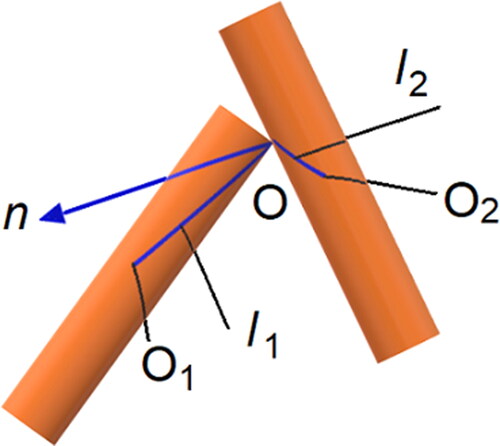
Particles would collide with each other and with the walls when they flow through a curved tube. Particles collision would affect the particle translation and rotation, which has an effect on the particle distribution and penetration efficiency. The collision of two cylindrical particles is assumed instantaneous and non-perfect elastic as shown in Figure 3 where the contact point and its normal direction n are determined by the relative position of two particles. In this article, cylindrical particle is modeled based on the slender-body theory in which a particle is divided into M segments. Each segment is considered as a sampled particle and participates in the judgment of collision between particles. In the process of integrating Equations (11)–(13), the variable time step is Δt = (u –${\mathit{v}}_p^i$)/$a_p^i,$ where u – ${\mathit{v}}_p^i$ is the velocity difference between fluid and particle, and $a_p^i$ is the acceleration of particle at time step i. At next time step i + 1, if the distance between the centroid of segment i of particle 1 and centroid of segment j of particle 2 is in ${\mathit{v}}_p^i$ the range of (d_p – d_p/10) to (d_p + d_p/10), it is determined that the two cylindrical particles will collide with each other. If the distance is less than (d_p – d_p/10), the original time step is reduced by half and recalculated. The collision point O is assumed to be at the midpoint of the line connecting the centroids of segment i and segment j. As shown in Figure 3, l₁ and l₂ are the vectors from centroids O₁ and O₂ of two particles to the contact point O, respectively, we define the normal direction n = l₁ + l₂. After collision, each particle attains an impulse I along the normal direction. The translational and angular velocities of two particles after collision depend on the impulse and are given as (17) $$I\mathit{n}+m_1{{\mathit{v}}_{\mathrm{p}}}_1=m_1{\mathit{v}}_{\mathrm{p}1}^{,},-I\mathit{n}+m_2{{\mathit{v}}_{\mathrm{p}}}_2=m_2{\mathit{v}}_{\mathrm{p}2}^{,},$$(17) where m and v_p are the mass and velocity of particle, respectively; subscript 1 and 2 is used to distinguish two particles, superscript “′” means after collision. Based on the law of collision, we have (18) $$e=-\frac{v_{\mathrm{p}2\mathrm{o}}^{,}-v_{\mathrm{p}1\mathrm{o}}^{,}}{v_{\mathrm{p}2\mathrm{o}}-v_{\mathrm{p}1\mathrm{o}}},$$(18) in which e is the restitution coefficient; v_p1o and v_p2o are the velocity components of two particles along the normal direction at contact point before collision. The torque exerted on the two particles is In × l₁ and –In × l₂, respectively. Then the rotation equation of particles is (19) $$I\mathit{n}\times {\mathit{l}}_1+J_1{\omega }_1=J_1{\omega }_1^{,},-I\mathit{n}\times l_2+J_2{\omega }_2=J_2{\omega }_2^{,},$$(19) then the impulse I can be written as: (20) $$I=\frac{m_1\left(1\mathrm{ }+\mathrm{ }e\right)\left(v_{\mathrm{p}2\mathrm{o}}-v_{\mathrm{p}1\mathrm{o}}\right)}{1\mathrm{ }+\mathrm{ }{m}_1/m_2\mathrm{ }+\mathrm{ }{m}_1\mathrm{ }\times \mathrm{ }{\left|\mathit{n} \times \mathrm{ }{\mathit{l}}_1\right|}^2/J_1+{ m}_1\mathrm{ }\times \mathrm{ }{\left|\mathit{n} \times \mathrm{ }{\mathit{l}}_2\right|}^2/J_2}.$$(20)

Figure 3. Schematic of collision of two cylindrical particles.

When particle 1 collides with the walls, the particle 2 can be regarded as wall and m₂ and v_p2 are taken as infinity and zero, respectively.

3.2. Flow field

For solving Equations (9)–(16), we should first obtain instantaneous velocity of fluid u which consists of mean velocity U and fluctuating velocity u′.

3.2.1. Coordinate transformation

As shown in Figure 1, the relationships of rectangular coordinate system with toroidal coordinate system are as follows: (21) $$x=\left(R-r\text{cos}\theta \right)\text{cos}\frac{S}{R},\mathrm{ }y=\left(R-r\text{cos}\theta \right)\text{sin}\frac{S}{R},\mathrm{ }z=r\text{sin}\theta .$$(21)

The orthonormal bases (e_r, e_θ, e_S) can be expressed with the rectangular Cartesian bases (i, j, k): (22) $${\mathit{e}}_r=-\mathit{i}\text{cos}\theta \text{cos}\frac{S}{R}-\mathit{j}\text{cos}\theta \text{sin}\frac{S}{R}+\mathit{k}\text{sin}\theta ,\mathrm{ }{\mathit{e}}_{\theta }=\mathit{i}\text{sin}\theta \text{cos}\frac{S}{R}+\mathit{j}\text{sin}\theta \text{sin}\frac{S}{R}+\mathit{k}\text{cos}\theta ,{\mathit{e}}_s=-\mathit{i}\text{sin}\frac{S}{R}+\mathit{j}\text{cos}\frac{S}{R}.$$(22)

3.2.2. Mean continuity and momentum equations

Mean velocity U is obtained by solving the mean continuity and momentum equations. The flow is assumed to be incompressible and fully developed turbulent flow, and corresponding governing equations are as follows: (23) $$\frac{\partial U_i}{\partial x_i}=0,$$(23) (24) $$U_j\frac{\partial U_i}{\partial x_j}=-\frac{1}{\rho }\frac{\partial P}{\partial x_i}+\nu \frac{{\partial }^2{U}_i}{{\partial }^2{x}_j}-\frac{\partial \overline{u_i^{\mathrm{\prime }}{u}_j^{\mathrm{\prime }}}}{\partial x_j},$$(24)

where U_i is the mean velocity and composed of three components U_r, U_θ and U_S; P is the mean pressure; ρ and ν are the fluid density and kinematic viscosity, respectively; $\overline{u_i^{\mathrm{\prime }}{u}_j^{\mathrm{\prime }}}$ is the Reynolds stress. Defining the mean axial velocity as (25) $${U_{\mathrm{S}}}_{\mathrm{c}}=\frac{B{a}^2}{4\mu },$$(25)

where $B=-\frac{\partial P}{\partial S};$ μ is the dynamic viscosity of fluid; a is the tube radius. We define the dimensionless pressure p, curvature κ, Reynolds number and Dean number as shown in Equation (26)(26) $$p=\frac{aP}{\mu U_{\mathrm{Sc}}},\mathrm{ }\kappa =\frac{a}{R},\mathrm{ }\mathrm{Re}=\frac{2U_{\mathrm{Sc}}a}{\nu },\mathrm{ }\text{De}=\mathrm{Re}\sqrt{\kappa },$$(26) , and non-dimensionalize Equation (24)(24) $$U_j\frac{\partial U_i}{\partial x_j}=-\frac{1}{\rho }\frac{\partial P}{\partial x_i}+\nu \frac{{\partial }^2{U}_i}{{\partial }^2{x}_j}-\frac{\partial \overline{u_i^{\mathrm{\prime }}{u}_j^{\mathrm{\prime }}}}{\partial x_j},$$(24) with a and U_Sc as shown in Equation (27)(27) $$\mathrm{Re}(U_j\frac{\partial U_i}{\partial x_j}+\frac{\partial \overline{u_i^{\mathrm{\prime }}{u}_j^{\mathrm{\prime }}}}{\partial x_j})=-\frac{\partial p}{\partial x_i}+\frac{{\partial }^2{U}_i}{{\partial }^2{x}_j}.$$(27) (26) $$p=\frac{aP}{\mu U_{\mathrm{Sc}}},\mathrm{ }\kappa =\frac{a}{R},\mathrm{ }\mathrm{Re}=\frac{2U_{\mathrm{Sc}}a}{\nu },\mathrm{ }\text{De}=\mathrm{Re}\sqrt{\kappa },$$(26) (27) $$\mathrm{Re}(U_j\frac{\partial U_i}{\partial x_j}+\frac{\partial \overline{u_i^{\mathrm{\prime }}{u}_j^{\mathrm{\prime }}}}{\partial x_j})=-\frac{\partial p}{\partial x_i}+\frac{{\partial }^2{U}_i}{{\partial }^2{x}_j}.$$(27)

3.2.3. Equations of Reynolds stress

The Reynolds stress in Equation (24)(24) $$U_j\frac{\partial U_i}{\partial x_j}=-\frac{1}{\rho }\frac{\partial P}{\partial x_i}+\nu \frac{{\partial }^2{U}_i}{{\partial }^2{x}_j}-\frac{\partial \overline{u_i^{\mathrm{\prime }}{u}_j^{\mathrm{\prime }}}}{\partial x_j},$$(24) is given by (28) $$\rho \frac{\partial \overline{u_i^{\mathrm{\prime }}{u}_j^{\mathrm{\prime }}}}{\partial t}+\rho U_k\frac{\partial \overline{u_i^{\mathrm{\prime }}{u}_j^{\mathrm{\prime }}}}{\partial x_k}=-\frac{\partial }{(\partial x_k)}(\rho \overline{u_i^{\mathrm{\prime }}{u}_j^{\mathrm{\prime }}{u}_k^{\mathrm{\prime }}}+{\delta }_{jk}\overline{u_i^{\mathrm{\prime }}{p}^{\mathrm{\prime }}}+{\delta }_{ik}\overline{u_j^{\mathrm{\prime }}{p}^{\mathrm{\prime }}}-\mu \frac{\partial \overline{u_i^{\mathrm{\prime }}{u}_j^{\mathrm{\prime }}}}{\partial x_k})－\rho (\overline{{\mathit{u}}_i^{\mathrm{\prime }}{\mathit{u}}_k^{\mathrm{\prime }}}\frac{\partial {\mathit{U}}_j}{\partial {\mathit{x}}_k}+\overline{{\mathit{u}}_j^{\mathrm{\prime }}{\mathit{u}}_k^{\mathrm{\prime }}}\frac{\partial {\mathit{U}}_i}{\partial {\mathit{x}}_k})-2\mu \overline{\frac{\partial {\mathit{u}}_i^{\mathrm{\prime }}}{\partial {\mathit{x}}_k}\frac{\partial {\mathit{u}}_j^{\mathrm{\prime }}}{\partial {\mathit{x}}_k}}+\overline{{\mathit{p}}^{\mathrm{\prime }}(\frac{\partial {\mathit{u}}_i^{\mathrm{\prime }}}{\partial {\mathit{x}}_j}+\frac{\partial {\mathit{u}}_j^{\mathrm{\prime }}}{\partial {\mathit{x}}_i})},$$(28) where p′ is the fluctuating pressure. The turbulent diffusion in the first term on the right-side hand of Equation (28)(28) $$\rho \frac{\partial \overline{u_i^{\mathrm{\prime }}{u}_j^{\mathrm{\prime }}}}{\partial t}+\rho U_k\frac{\partial \overline{u_i^{\mathrm{\prime }}{u}_j^{\mathrm{\prime }}}}{\partial x_k}=-\frac{\partial }{(\partial x_k)}(\rho \overline{u_i^{\mathrm{\prime }}{u}_j^{\mathrm{\prime }}{u}_k^{\mathrm{\prime }}}+{\delta }_{jk}\overline{u_i^{\mathrm{\prime }}{p}^{\mathrm{\prime }}}+{\delta }_{ik}\overline{u_j^{\mathrm{\prime }}{p}^{\mathrm{\prime }}}-\mu \frac{\partial \overline{u_i^{\mathrm{\prime }}{u}_j^{\mathrm{\prime }}}}{\partial x_k})－\rho (\overline{{\mathit{u}}_i^{\mathrm{\prime }}{\mathit{u}}_k^{\mathrm{\prime }}}\frac{\partial {\mathit{U}}_j}{\partial {\mathit{x}}_k}+\overline{{\mathit{u}}_j^{\mathrm{\prime }}{\mathit{u}}_k^{\mathrm{\prime }}}\frac{\partial {\mathit{U}}_i}{\partial {\mathit{x}}_k})-2\mu \overline{\frac{\partial {\mathit{u}}_i^{\mathrm{\prime }}}{\partial {\mathit{x}}_k}\frac{\partial {\mathit{u}}_j^{\mathrm{\prime }}}{\partial {\mathit{x}}_k}}+\overline{{\mathit{p}}^{\mathrm{\prime }}(\frac{\partial {\mathit{u}}_i^{\mathrm{\prime }}}{\partial {\mathit{x}}_j}+\frac{\partial {\mathit{u}}_j^{\mathrm{\prime }}}{\partial {\mathit{x}}_i})},$$(28) can be modified as (Lien and Leschziner 1994) (29) $$\rho \overline{{\mathrm{u}}_{\mathrm{i}}^{\mathrm{\prime }}{\mathrm{u}}_{\mathrm{j}}^{\mathrm{\prime }}{\mathrm{u}}_{\mathrm{k}}^{\mathrm{\prime }}}+{\delta }_{\mathrm{j}\mathrm{k}}\overline{{\mathrm{u}}_{\mathrm{i}}^{\mathrm{\prime }}{\mathrm{p}}^{\mathrm{\prime }}}+{\delta }_{\mathrm{i}\mathrm{k}}\overline{{\mathrm{u}}_{\mathrm{j}}^{\mathrm{\prime }}{\mathrm{p}}^{\mathrm{\prime }}}=\frac{{\mu }_{\mathrm{t}}}{{\sigma }_{\mathrm{k}1}}\frac{\partial \overline{{\mathrm{u}}_{\mathrm{i}}^{\mathrm{\prime }}{\mathrm{u}}_{\mathrm{j}}^{\mathrm{\prime }}}}{\partial {\mathrm{x}}_{\mathrm{k}}},$$(29)

where σ_k1= 0.82, μ_t = ρC_μk²/ε (C_μ = 0.09,$k=\overline{u_i^{\prime }{u}_i^{\prime }}/2$ is the turbulent kinetic energy, ε is the turbulent dissipation rate. The diffusion term in the third term on the right-side hand of Equation (28)(28) $$\rho \frac{\partial \overline{u_i^{\mathrm{\prime }}{u}_j^{\mathrm{\prime }}}}{\partial t}+\rho U_k\frac{\partial \overline{u_i^{\mathrm{\prime }}{u}_j^{\mathrm{\prime }}}}{\partial x_k}=-\frac{\partial }{(\partial x_k)}(\rho \overline{u_i^{\mathrm{\prime }}{u}_j^{\mathrm{\prime }}{u}_k^{\mathrm{\prime }}}+{\delta }_{jk}\overline{u_i^{\mathrm{\prime }}{p}^{\mathrm{\prime }}}+{\delta }_{ik}\overline{u_j^{\mathrm{\prime }}{p}^{\mathrm{\prime }}}-\mu \frac{\partial \overline{u_i^{\mathrm{\prime }}{u}_j^{\mathrm{\prime }}}}{\partial x_k})－\rho (\overline{{\mathit{u}}_i^{\mathrm{\prime }}{\mathit{u}}_k^{\mathrm{\prime }}}\frac{\partial {\mathit{U}}_j}{\partial {\mathit{x}}_k}+\overline{{\mathit{u}}_j^{\mathrm{\prime }}{\mathit{u}}_k^{\mathrm{\prime }}}\frac{\partial {\mathit{U}}_i}{\partial {\mathit{x}}_k})-2\mu \overline{\frac{\partial {\mathit{u}}_i^{\mathrm{\prime }}}{\partial {\mathit{x}}_k}\frac{\partial {\mathit{u}}_j^{\mathrm{\prime }}}{\partial {\mathit{x}}_k}}+\overline{{\mathit{p}}^{\mathrm{\prime }}(\frac{\partial {\mathit{u}}_i^{\mathrm{\prime }}}{\partial {\mathit{x}}_j}+\frac{\partial {\mathit{u}}_j^{\mathrm{\prime }}}{\partial {\mathit{x}}_i})},$$(28) is given as (30) $$2\mu \overline{\frac{\partial u_i^{\mathrm{\prime }}}{\partial x_k}\frac{\partial u_j^{\mathrm{\prime }}}{\partial x_k}}=\frac{2}{3}{\delta }_{ij}\rho \epsilon .$$(30)

The pressure–strain term in the last term on the right-side hand of Equation (28)(28) $$\rho \frac{\partial \overline{u_i^{\mathrm{\prime }}{u}_j^{\mathrm{\prime }}}}{\partial t}+\rho U_k\frac{\partial \overline{u_i^{\mathrm{\prime }}{u}_j^{\mathrm{\prime }}}}{\partial x_k}=-\frac{\partial }{(\partial x_k)}(\rho \overline{u_i^{\mathrm{\prime }}{u}_j^{\mathrm{\prime }}{u}_k^{\mathrm{\prime }}}+{\delta }_{jk}\overline{u_i^{\mathrm{\prime }}{p}^{\mathrm{\prime }}}+{\delta }_{ik}\overline{u_j^{\mathrm{\prime }}{p}^{\mathrm{\prime }}}-\mu \frac{\partial \overline{u_i^{\mathrm{\prime }}{u}_j^{\mathrm{\prime }}}}{\partial x_k})－\rho (\overline{{\mathit{u}}_i^{\mathrm{\prime }}{\mathit{u}}_k^{\mathrm{\prime }}}\frac{\partial {\mathit{U}}_j}{\partial {\mathit{x}}_k}+\overline{{\mathit{u}}_j^{\mathrm{\prime }}{\mathit{u}}_k^{\mathrm{\prime }}}\frac{\partial {\mathit{U}}_i}{\partial {\mathit{x}}_k})-2\mu \overline{\frac{\partial {\mathit{u}}_i^{\mathrm{\prime }}}{\partial {\mathit{x}}_k}\frac{\partial {\mathit{u}}_j^{\mathrm{\prime }}}{\partial {\mathit{x}}_k}}+\overline{{\mathit{p}}^{\mathrm{\prime }}(\frac{\partial {\mathit{u}}_i^{\mathrm{\prime }}}{\partial {\mathit{x}}_j}+\frac{\partial {\mathit{u}}_j^{\mathrm{\prime }}}{\partial {\mathit{x}}_i})},$$(28) consists of the slow pressure–strain, rapid pressure–strain and wall reflection term (Launder 1989a,b) (31) $$\overline{p^{\mathrm{\prime }}(\frac{\partial u_i^{\mathrm{\prime }}}{\partial x_j}+\frac{\partial u_j^{\mathrm{\prime }}}{\partial x_i})}=-C_1\rho \frac{\epsilon }{k}[\overline{u_i^{\mathrm{\prime }}{u}_j^{\mathrm{\prime }}}-\frac{2}{3}{\delta }_{ij}k]-C_2\left[\right(P_{ij}-C_{ij})-\frac{2}{3}{\delta }_{ij}(P_k-C_k\left)\right]-C_1^{\mathrm{\prime }}\frac{\epsilon }{k}(\overline{u_k^{\mathrm{\prime }}{u}_m^{\mathrm{\prime }}}{n}_k{n}_m{\delta }_{ij}-\frac{3}{2}\overline{u_i^{\mathrm{\prime }}{u}_k^{\mathrm{\prime }}}{n}_j{n}_k-\frac{3}{2}\overline{u_j^{\mathrm{\prime }}{u}_k^{\mathrm{\prime }}}{n}_i{n}_k)\frac{k^{\frac{3}{2}}}{C_l\epsilon d}+C_2^{\mathrm{\prime }}({\phi }_{km,2}{n}_k{n}_m{\delta }_{ij}-\frac{3}{2}{\phi }_{ik,2}{n}_j{n}_k-\frac{3}{2}{\phi }_{j\mathrm{k},2}{n}_i{n}_k)\frac{k^{\frac{3}{2}}}{C_l\epsilon d},$$(31) where C₁ = 1.8, C₂ = 0.60, $C_1^{\prime }$ = 0.5, $C_2^{\prime }$ = 0.3, C_l = $C_{\mu }^{3/4}$/0.04187; n_k is the component vertical to the wall; d is the distance from the wall; C_ij, C_k, P_ij, P_k and ϕ_km,2 are as follows: (32) $$C_{ij}=\rho U_k\frac{\partial \overline{u_i^{\mathrm{\prime }}{u}_j^{\mathrm{\prime }}}}{\partial x_k},\mathrm{ }{C}_k=\rho U_k\frac{\partial \overline{u_i^{\mathrm{\prime }}{u}_i^{\mathrm{\prime }}}}{\partial x_k},\mathrm{ }{P}_{ij}=-\rho \left(\overline{u_i^{\mathrm{\prime }}{u}_k^{\mathrm{\prime }}}\frac{\partial U_j}{\partial x_k}+\overline{u_j^{\mathrm{\prime }}{u}_k^{\mathrm{\prime }}}\frac{\partial U_i}{\partial x_k}\right),\mathrm{ }{P}_k=-\rho \overline{u_i^{\mathrm{\prime }}{u}_l^{\mathrm{\prime }}}\frac{\partial U_i}{\partial x_l},\mathrm{ }{\varphi }_{km,2}=-C_2\left[\right(P_{km}-C_{km})-\frac{2}{3}{\delta }_{km}(P_k-C_k\left)\right].$$(32)

The modified equations of k and ε included in the above equations are (33) $$\rho \frac{\partial k}{\partial t}+\rho U_j\frac{\partial k}{\partial x_j}=-\rho \overline{u_i^{\mathrm{\prime }}{u}_j^{\mathrm{\prime }}}\frac{\partial U_i}{\partial x_j}-\rho \epsilon +\frac{\partial }{\partial x_j}\left[\right(\mu +\frac{{\mu }_t}{{\sigma }_{k2}}\left)\frac{\partial k}{\partial x_j}\right],$$(33) (34) $$\rho \frac{\partial \epsilon }{\partial t}+\rho U_j\frac{\partial \epsilon }{\partial x_j}=\frac{\partial }{\partial x_j}\left[\right(\mu +\frac{{\mu }_t}{{\sigma }_{\epsilon }}\left)\frac{\partial \epsilon }{\partial x_j}\right]+C_{\epsilon 1}{P}_k\frac{\epsilon }{k}-C_{\epsilon 2}\rho \frac{{\epsilon }^2}{k},$$(34) where C_ε1 = 1.44, C_ε2 = 1.92, σ_k2 = 1.0, σ_ε = 1.3.

3.2.4. Fluctuating fluid velocity

The turbulent diffusion is reflected by the fluctuating fluid velocity u′. A turbulent flow can be represented in the Fourier modes, the expression of one point velocity correlation and the scalar energy spectrum. The dynamical interactions between different modes and the kinematic process of advection of the vorticity field can be simulated by the velocity field in a homogeneous isotropic turbulence. Kolmogorov’s hypothesis of local isotropic turbulence states the small-scale turbulent motions are statistically isotopic. The fluid fluctuating velocity u′ is related to the small-scale turbulent motions. Therefore, the homogeneous isotropic turbulence model is chosen to obtain the fluid fluctuating velocity. However, it should be pointed out that the turbulence in the boundary layer near the wall is highly anisotropic, and particle deposition is highly affected by the anisotropic feature. Therefore, such anisotropic effect on the fluid fluctuating velocity is worthy of further study in the future. In order to obtain the fluid fluctuating velocity u′, we represent u′ with a Fourier series using the kinetic simulation sweeping model as (Wang and Stock 1994; Fung et al. 1992) follows: (35) $$\mathit{u}\mathrm{\prime }\left(x,t\right)=\sum _{n=1}^N{\mathit{\xi }}^{\left(n\right)}\times \frac{{\mathit{k}}^{\left(n\right)}}{\left|{\mathit{k}}^{\left(n\right)}\right|}\text{sin}\left({\mathit{k}}^{\left(n\right)}x+{\omega }^{\left(n\right)}t\right)+{\mathit{\zeta }}^{\left(n\right)}\times \frac{{\mathit{k}}^{\left(n\right)}}{\left|{\mathit{k}}^{\left(n\right)}\right|}\text{cos}\left({\mathit{k}}^{\left(n\right)}x+{\omega }^{\left(n\right)}t\right),$$(35)

where ξ⁽ⁿ⁾ and ζ⁽ⁿ⁾ are the random vectors obeying the Gaussian distribution with the mean value of zero and standard deviation of $(\frac{\overline{u_i^{\mathrm{\prime }}{u}_i^{\mathrm{\prime }}}}{2N{)}^{1/2}};$ N is a constant (N = 100 here); frequency ω⁽ⁿ⁾ is a Gaussian random number with the standard deviation being the root-mean-square of u′; the wave number vector k⁽ⁿ⁾ is an isotropic random vector on the surface of unit sphere. ω⁽ⁿ⁾ and the distribution functions of radius k⁽ⁿ⁾ are determined by: (36) $$E\left(k\right)=\frac{3u_0^2}{2\pi }\frac{k^4}{k_0^5{\left[1+\frac{k^2}{\left(4k_0^2\right)}\right]}^4},D\left(\tau \right)=\hspace{0.17em}\text{cos}\hspace{0.17em}({\omega }_0\tau )\exp (-{\omega }_0\tau ),$$(36) where E(k) is the Karman–Pao energy spectrum of turbulence; D(τ) is the second-order correlation function. Then ω⁽ⁿ⁾ and k⁽ⁿ⁾ obey the Cauchy distribution: (37) $$P_{1i}\left(k_i\right)=\frac{1}{\pi k_0\left[1+\frac{k_i^2}{k_0^2}\right]},P_2\left(\omega \right)=\frac{1}{\pi {\omega }_0\left[1+\frac{{\omega }^2}{{\omega }_0^2}\right]}.$$(37)

The turbulent flow can be determined by $\overline{u_i^{\mathrm{\prime }}{u}_i^{\mathrm{\prime }}},$ ω₀ and k₀ based on Equation (37)(37) $$P_{1i}\left(k_i\right)=\frac{1}{\pi k_0\left[1+\frac{k_i^2}{k_0^2}\right]},P_2\left(\omega \right)=\frac{1}{\pi {\omega }_0\left[1+\frac{{\omega }^2}{{\omega }_0^2}\right]}.$$(37) . For the Karman–Pao spectrum, k₀ = 1/L_f and ω₀ = 0.5/T_mE with L_f and T_mE being the Lagrangian integral length and Eulerian integral time scale, respectively (Dong et al. 2003): (38) $$L_{\mathrm{f}}=\frac{0.16k^{\frac{3}{2}}}{\epsilon },T_{\mathrm{mE}}=\frac{k}{\epsilon }.$$(38)

4. Numerical simulation

4.1. Main steps of simulation

(1) Solve Equations (23)(23) $$\frac{\partial U_i}{\partial x_i}=0,$$(23) and (34)(34) $$\rho \frac{\partial \epsilon }{\partial t}+\rho U_j\frac{\partial \epsilon }{\partial x_j}=\frac{\partial }{\partial x_j}\left[\right(\mu +\frac{{\mu }_t}{{\sigma }_{\epsilon }}\left)\frac{\partial \epsilon }{\partial x_j}\right]+C_{\epsilon 1}{P}_k\frac{\epsilon }{k}-C_{\epsilon 2}\rho \frac{{\epsilon }^2}{k},$$(34) to obtain U_i, k and ε.

(2) Solve Equations (35)–(38) to obtain u′.

(3) Initialize particle position, orientation, velocity and angular velocity.

(4) Calculate η and ε using Equations (3)(3) $$A=\left|\begin{array}{ccc}1-2\left({\epsilon }_2^2+{\epsilon }_3^2\right)& 2\left({\epsilon }_1{\epsilon }_2+{\epsilon }_3\eta \right)& 2\left({\epsilon }_1{\epsilon }_3-{\epsilon }_2\eta \right)\\ 2\left({\epsilon }_1{\epsilon }_2-{\epsilon }_3\eta \right)& 1-2\left({\epsilon }_3^2+{\epsilon }_1^2\right)& 2\left({\epsilon }_2{\epsilon }_3+{\epsilon }_1\eta \right)\\ 2\left({\epsilon }_1{\epsilon }_3+{\epsilon }_2\eta \right)& 2\left({\epsilon }_2{\epsilon }_3-{\epsilon }_1\eta \right)& 1-2\left({\epsilon }_1^2+{\epsilon }_2^2\right)\end{array}\right|.$$(3) and (4)(4) $$\left|\begin{array}{c}{\epsilon }_1\\ {\epsilon }_2\\ {\epsilon }_3\end{array}\right|=\frac{1}{4\eta }|\begin{array}{c}{a}_{23}-a_{32}\\ a_{31}-a_{13}\\ a_{12}-a_{21}\end{array}|=\frac{1}{4\eta }|\begin{array}{c}-\text{sin}\psi \text{sin}\phi \\ \text{sin}\psi \left(\text{cos}\phi +1\right)\\ \text{sin}\phi \left(\text{cos}\psi +1\right)\end{array}|,\mathrm{ }\eta =\sqrt{1+a_{11}+a_{22}+a_{33}},$$(4) .

(5) Calculate transform matrix A using Equation (5)(5) $${\epsilon }_1=\sqrt{\frac{1+a_{11}}{2}},\mathrm{ }{\epsilon }_2=\frac{a_{12}}{2{\epsilon }_1},\mathrm{ }{\epsilon }_3=\frac{a_{23}}{2{\epsilon }_2},\mathrm{ }\text{when}\mathrm{ }\eta \mathrm{ }=\mathrm{ }0.$$(5) .

(6) Calculate F and L using Equations (9)(9) $$\mathit{u}({\mathit{x}}_{\mathrm{c}}+l{s}_i\mathit{p})-[{\mathit{v}}_{\mathrm{p}}+(\mathit{\omega }\times l{s}_i\mathit{p}\left)\right]=-\left[2\right(\ln 2\beta +\ln \sqrt{1-s_i^2}\left)\right(\mathit{\delta }+\mathit{pp})+(\mathit{\delta }-3\mathit{p}\mathit{p}\left)\right]\cdot \mathit{f}\left(s_i\right)+{\sum }_{\begin{array}{c}m=1\\ m\ne i\end{array}}^M\frac{l_m}{\left|s_i-s_m\right|}(\mathit{\delta }+\mathit{pp})\cdot \mathit{f}\left(s_i\right)-{\sum }_{\begin{array}{c}m=1\\ m\ne i\end{array}}^M{k}_{im}=\frac{l_m}{\left|s_i-s_m\right|}(\mathit{\delta }+\mathit{pp})\cdot \mathit{f}\left(s_m\right)\hspace{1em}(i=1,2,\dots ,M),$$(9) and (10)(10) $$F=8\pi \mu l{\int }_{-1}^{1}f\left(s\right)ds, L=8\pi \mu l^2{\int }_{-1}^{1}sp\times f\left(s\right)ds.$$(10) .

(7) Transform L from the coordinate system-xyz to -123 using Equation (14)(14) $$\left|\begin{array}{c}{L}_1\\ L_2\\ L_3\end{array}\right|=|\begin{array}{c}{a}_{11}\mathrm{ }{a}_{12}\mathrm{ }{a}_{13}\\ a_{21}\mathrm{ }{a}_{22}\mathrm{ }{a}_{23}\\ a_{31}\mathrm{ }{a}_{32}\mathrm{ }{a}_{33}\end{array}||\begin{array}{c}{T}_x\\ T_y\\ T_z\end{array}|.$$(14) .

(8) Calculate particle position and orientation at next time step using Equations (6)(6) $$\left|\begin{array}{c}\frac{d\eta }{dt}\\ \frac{d{\epsilon }_1}{dt}\\ \frac{d{\epsilon }_2}{dt}\\ \frac{d{\epsilon }_3}{dt}\end{array}\right|=\frac{1}{2}|\begin{array}{c}-{\epsilon }_1{\omega }_1-{\epsilon }_2{\omega }_2-{\epsilon }_3{\omega }_3\\ \eta {\omega }_1-{\epsilon }_3{\omega }_2+{\epsilon }_2{\omega }_3\\ {\epsilon }_3{\omega }_1+\eta {\omega }_2-{\epsilon }_1{\omega }_3\\ -{\epsilon }_2{\omega }_1+{\epsilon }_1{\omega }_2+\eta {\omega }_3\end{array}|,\mathrm{ }$$(6) , (11)–(13) and (15)–(16).

(9) Return to step (4(4) $$\left|\begin{array}{c}{\epsilon }_1\\ {\epsilon }_2\\ {\epsilon }_3\end{array}\right|=\frac{1}{4\eta }|\begin{array}{c}{a}_{23}-a_{32}\\ a_{31}-a_{13}\\ a_{12}-a_{21}\end{array}|=\frac{1}{4\eta }|\begin{array}{c}-\text{sin}\psi \text{sin}\phi \\ \text{sin}\psi \left(\text{cos}\phi +1\right)\\ \text{sin}\phi \left(\text{cos}\psi +1\right)\end{array}|,\mathrm{ }\eta =\sqrt{1+a_{11}+a_{22}+a_{33}},$$(4) ) until the particles move out of the tube or deposit on the walls.

(10) Calculate the penetration efficiency of particles Pe = N_out/N_in, where N_out and N_in are the particle number at outlet and at the entrance of the tube, respectively.

4.2. Numerical method and parameters

A finite volume method is used in the solver to solve Equations (15)–(16) and (23)–(34). The SIMPLE scheme is employed to deal with the term of velocity–pressure coupling, and the convection term is discretized with the power-law scheme which is a piece-wise approximation to the exact solution of a one-dimensional convection–diffusion type of equation, and always leads to physically realistic solution. A staggered mesh system is used in the simulation. The pressure, axial velocity U_S are located at the centroids of the control volumes, whereas the velocity components U_r and U_θ over the cross-section are located at the boundary. The no-slip condition is used on the walls. The standard wall function is used and the distance of the first cell centroid from a wall is laid at y⁺ = 30. Equation (6)(6) $$\left|\begin{array}{c}\frac{d\eta }{dt}\\ \frac{d{\epsilon }_1}{dt}\\ \frac{d{\epsilon }_2}{dt}\\ \frac{d{\epsilon }_3}{dt}\end{array}\right|=\frac{1}{2}|\begin{array}{c}-{\epsilon }_1{\omega }_1-{\epsilon }_2{\omega }_2-{\epsilon }_3{\omega }_3\\ \eta {\omega }_1-{\epsilon }_3{\omega }_2+{\epsilon }_2{\omega }_3\\ {\epsilon }_3{\omega }_1+\eta {\omega }_2-{\epsilon }_1{\omega }_3\\ -{\epsilon }_2{\omega }_1+{\epsilon }_1{\omega }_2+\eta {\omega }_3\end{array}|,\mathrm{ }$$(6) is calculated using the trapezoid formula to obtain the particle displacement and the derivatives of Euler parameters. Equations (11)–(13) is integrated using the explicit Euler formula to get the particle velocity and angular velocity at next time step. The particle velocity at time step i + 1 is obtained after Δt is calculated. Parameters used in the computation are: ρ = 1.205 kg/m³, μ = 1.808 × 10^–5Pa s, T = 293 K, k_B = 1.38 × 10^–23J/K, λ = 6.9 × 10^–8 m, e = 0.37. About 20,000 cylindrical particles with isotropic orientation angle are initially distributed homogenously on the cross-section at the entrance.

Definitions of Reynolds number, Dean number and curvature κ are shown in Equation (26(26) $$p=\frac{aP}{\mu U_{\mathrm{Sc}}},\mathrm{ }\kappa =\frac{a}{R},\mathrm{ }\mathrm{Re}=\frac{2U_{\mathrm{Sc}}a}{\nu },\mathrm{ }\text{De}=\mathrm{Re}\sqrt{\kappa },$$(26) ), and the Stokes number is defined as the ratio of particle respond time to characteristic time of the flow: (39) $$\mathrm{St}=\frac{{\rho }_{\mathrm{p}}{u}_{\tau }^2{d_{\mathrm{p}}}^2{C}_{\mathrm{c}}}{18\rho {\nu }^2},\mathrm{ }{u}_{\tau }=\sqrt{\frac{0.04}{{\mathrm{Re}}^{1/4}}}{U}_{\mathrm{Sc}},$$(39) where ρ_p is the particle density; u_τ is the friction velocity; C_c is the Cunningham slip correction factor as shown in Equation (13)(13) $$C_{\mathrm{c}}=1+2.257\left(\frac{2\lambda }{d_{\mathrm{pe}}}\right)+0.4\left(\frac{2\lambda }{d_{\mathrm{pe}}}\right)\exp (\frac{\mathrm{–}0.55d_{\mathrm{pe}}}{\lambda }),$$(13) .

4.3. Mesh independence test and validation

The number of grid cells is 128(r) × 128(θ) × 256(S) grid points. A uniform grid was employed in the θ and S directions, while grids are clustered close to the wall in the r direction. A grid independence test is performed by changing grid points from 96 to 160 in the r and θ directions, 224 to 288 in the S direction, respectively. A convergence criterion is specified with all the normalized residual errors for each physical quantity being less than 10^–4.

In order to validate the model and numerical method, we compare the present numerical results of mean axial velocity and root-mean-square (RMS) value of fluctuating axial velocity with the experimental results (Webster and Humphrey 1993) along the tube midplane (white line) at the outlet as shown in Figure 4. The experiment was carried out in a tube of 40 tube diameters in length and of inner diameter 3.81 ± 0.05 cm using the laser Doppler velocimeter. The numerical results are qualitatively consistent with the experimental ones.

Figure 4. Distribution of mean axial velocity (a) and RMS value of fluctuating axial velocity (b) along the tube midplane (white line) (Re = 10,500, De = 2460).

5. Results and discussion

The computations are performed for a 90° curved tube with the centerline length of L_b = πR/2.

5.1. Distribution of particles at different axial positions

5.1.1. Number concentration

Contours of relative particle number concentration on the cross-section at different axial positions are shown in Figure 5 where the depth of color represents the value of the particle number concentration, and the darkest color corresponds to the maximum concentration. The uniform distribution of number concentration at the entrance turns to be non-uniform along the flow direction because particle motion is controlled by the drag force, centrifugal force and random force as shown in Equation (11)(11) $$m\frac{d{v}_{\mathrm{p}}}{dt}=\frac{F}{C_c}+m\frac{v_{\mathrm{p}S}^2}{(R+r)}+{\mathit{R}}_{\mathrm{b}}\sqrt{\frac{6\pi d_{\mathrm{pe}}{k}_{B}T\mu }{\mathrm{\Delta }t}},$$(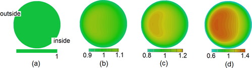11) . The non-uniformity increases with the increase of the axial distance. The distribution of particle number concentration is symmetric about the tube midplane, but asymmetrically in the left and right part because of the effect of the inertia and the secondary flow. More particles accumulate in the region closer to the outside of the tube. The maximum of particle number concentration is located in the region where the fluid mean axial velocity is large and the RMS value of fluctuating axial velocity is small as shown in Figure 4. Generally, the random force results in a uniform distribution of the particle number concentration, so the non-uniform distribution of particle number concentration is caused by the drag force and the centrifugal force.

Figure 5. Distribution of relative particle number concentration on the cross-section at different axial positions (Re = 10,500, St = 0.014, De = 1862, β = 8). (a) S/L_b =0, (b) S/L_b =1/3, (c) S/L_b =2/3, and (d) S/L_b = 1.

5.1.2. Orientation angle

Figure 6 shows the distributions of mean orientation of particles on the cross-section at different axial positions. In the figure ϕ is an angle between the particle major axis and the local streamline, and is obtained by averaging the orientation angles on the cross-section at a fixed axial position. The localized flow velocity vector can be calculated with the values of three components of localized flow velocity, and orientation vector of particle can be obtained by solving Equation (15)(15) $$\frac{\partial \mathrm{\Psi }}{\partial t}=-\nabla \cdot \left(\mathit{\omega }\mathrm{\Psi }\right)+\nabla \cdot (D\nabla \mathrm{\Psi }),$$(15) of orientation distribution function. We can see that the mean orientation angles change from isotropic distribution at the entrance to non-isotropic distribution along the flow direction. The particles gradually align with their major axis near to the flow direction. As shown in Equations (12)–(16), the particle orientation is controlled by the torque exerted on the particle by the fluid and the Brownian diffusion. The latter makes the distribution of particle orientation become more isotropic, so alignment of particles near to the flow direction results from the torque which consists of two parts, one making particle rotate around the vorticity axis, and another causing particle spin around and align with the flow direction.

Figure 6. Distributions of mean orientation of particles on the cross-section at different axial positions. (Re = 10,500, St = 0.014, De = 1862, β = 8).

5.2. Distribution of particles at outlet

5.2.1. Number concentration

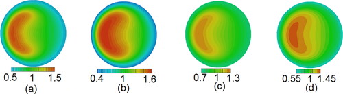
Figure 7 shows the contours of relative particle number concentration on the cross-section at outlet for different Stokes number, Dean number, Reynolds number and particle aspect ratio. Comparing the cases with different Stokes number between Figure 7a and Figure 5d, it can be seen that the non-uniformity increases with increasing Stokes number. As we know, the Stokes number is directly proportional to the particle inertia. It is easier for the particles with larger Stokes number to accumulate in the region closer to the outside of the tube because of larger inertial centrifugal force. The difference in the particle number concentration for different Dean number can be observed by comparing Figure 7b and Figure 5d. Larger Dean number corresponds to a larger curvature κ when the Reynolds number is fixed as shown in Equation (26)(26) $$p=\frac{aP}{\mu U_{\mathrm{Sc}}},\mathrm{ }\kappa =\frac{a}{R},\mathrm{ }\mathrm{Re}=\frac{2U_{\mathrm{Sc}}a}{\nu },\mathrm{ }\text{De}=\mathrm{Re}\sqrt{\kappa },$$(26) . Larger curvature means a larger inertial centrifugal force when particles pass through a curved tube, so that the non-uniformity increases with the increase of the Dean number. The comparison of particle number concentration for different Reynolds number is shown in Figure 7c and Figure 5d where we can see that the non-uniformity increases with increasing Reynolds number. A stronger secondary flow would appear in the flow with larger Reynolds number, which drives the particles to move to the near-wall region. Figure 7d and Figure 5d show the comparison of particle number concentration for different particle aspect ratio. The particles with larger aspect ratio experience a larger inertial centrifugal force and smaller random force, so the distribution of particle number concentration is more uniform for the particles with larger aspect ratio.

Figure 7. Distribution of relative particle number concentration on the cross-section at outlet. (a) St = 0.020, De = 1862, Re = 10,500, β = 8, (b) St = 0.014, De = 2460, Re = 10,500, β = 8, (c) St = 0.014, De = 1862, Re = 4500, β = 8, and (d) St = 0.014, De = 1862, Re = 10,500, β = 4.

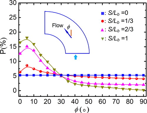
5.2.2. Orientation angle

Effects of Stokes number and Dean number on the distributions of mean orientation of particles on the cross-section at outlet are shown in Figures 8 and 9, respectively. In Figure 8, the phenomenon that particles align with their major axis near to the flow direction is more obvious with increasing Stokes number. The reason can be analyzed as follows. Particle orientation is controlled by the fluid drag force and Brownian random force as shown in Equations (15)(15) $$\frac{\partial \mathrm{\Psi }}{\partial t}=-\nabla \cdot \left(\mathit{\omega }\mathrm{\Psi }\right)+\nabla \cdot (D\nabla \mathrm{\Psi }),$$(15) and (16)(16) $$D=\frac{k_{B}T}{R_{\mathrm{r}}},R_{\mathrm{r}}=\frac{8\pi \rho \nu l^3}{3\ln (\frac{4l}{d_{\mathrm{pe}}})},$$(16) . The Brownian random force makes particles orient more isotropically, weakening the preferred orientation, while the effect of the Brownian random force is relatively weak for the particles with larger Stokes number.

Figure 8. Distribution of particle orientation for different St (Re = 10,500, De = 1862, β = 8).

Figure 9. Distribution of particle orientation for different De (Re = 10,500, St = 0.014, β = 8).

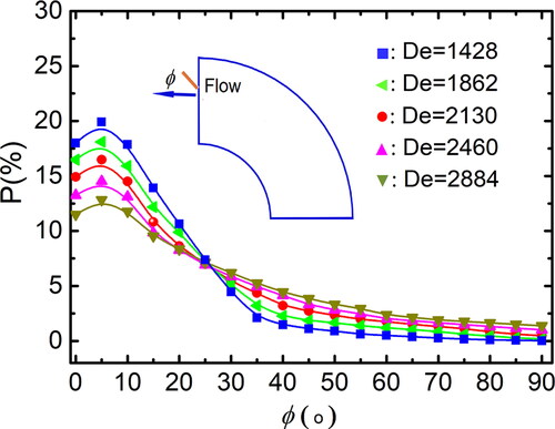
In Figure 9, fewer particles align with their major axis near to the flow direction with increasing Dean number. As we know, the strength of the induced secondary flow in the curved tube increases with the increase of curvature which is directly proportional to the Dean number as shown in Equation (26)(26) $$p=\frac{aP}{\mu U_{\mathrm{Sc}}},\mathrm{ }\kappa =\frac{a}{R},\mathrm{ }\mathrm{Re}=\frac{2U_{\mathrm{Sc}}a}{\nu },\mathrm{ }\text{De}=\mathrm{Re}\sqrt{\kappa },$$(26) , while the force exerted on the particles by the secondary flow prevents the particle major axis from aligning near to the flow direction.

Distributions of mean orientation of particles on the cross-section at outlet for different Reynolds number and particle aspect ratio are shown in Figures 10 and 11, respectively. As shown in Equations (9)–(11), the torque exerted on the particle is resulted from the difference between the particle velocity and fluid instantaneous velocity which consists of mean velocity U and fluctuating velocity u′. The mean velocity as well as its induced shear rate causes the particles to rotate and orient toward a flow-related direction, while random fluctuating velocity causes the particles to rotate and orient isotropically. The Reynolds number is the most important parameter to characterize turbulent flow. The larger the Reynolds number is, the smaller the scale of minimum vortex is, the wider the distribution of energy spectrum contained in the vortices of different scales is, and the stronger the effect of random fluctuating velocity is. So the phenomenon that particles align near to the flow direction is less obvious. On the other hand, a stronger secondary flow would appear in the flow when the Reynolds number is larger, which also prevents the particle major axis from aligning near to the flow direction.

Figure 10. Distribution of particle orientation for different Re (De = 1862, St = 0.014, β = 8).

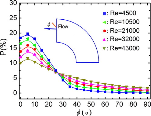
Figure 11. Distribution of particle orientation for different aspect ratio (Re = 10,500, De = 1862, St = 0.014).

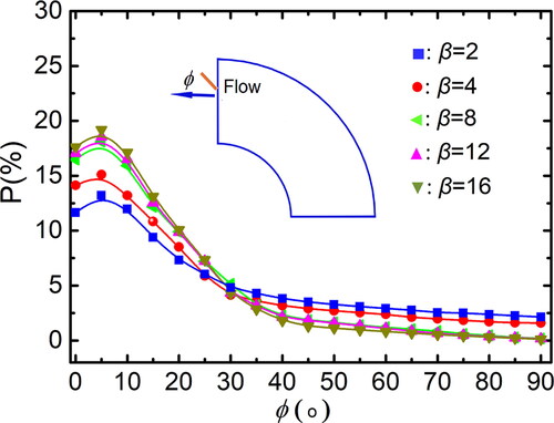
In Figure 11, more particles tend to align with their major axis near to the flow direction with increasing particle aspect ratio. The torque exerted on the particle is related to vertical scale, i.e., large and small scale vortices respond to the mean velocity U and fluctuating velocity u′, respectively. The particles with small aspect ratio are affected greatly by the random fluctuating velocity u′ which corresponds to the small scale vortices, so the preferential orientation toward the flow direction is less obvious. In addition, the difference in the distributions of mean orientation of particles between the cases with different aspect ratio is small for large aspect ratio, which is consistent with the conclusion (Krushkal and Gallily 1988) that the orientation distribution is not sensitive to the aspect ratio for the particles with aspect ratio larger than 5.

5.3. Penetration efficiency

Penetration efficiency is directly related to the particle deposition. Here a cylindrical particle is modeled based on the slender-body theory in which a particle is divided into N segments. Each segment is considered as a sampled particle and participates in the judgment of collision with the walls. If the distance between the centroid of a particle segment and wall is less than d_p/2, it is determined that the particles collide with the wall. Particle which strikes a wall will deposit to it at low collision velocity because the kinetic energy of a particle is not large enough to escape the attractive forces at the wall. In the simulation, the particle is considered to be deposited to the wall when the component of particle velocity perpendicular to the wall after collision is less than or equal to zero. The number of particle deposition is dependent on the particle trajectory which is controlled by the various forces, torques and particle aspect ratio as shown in Equations (11)–(13). The secondary flow enhances the transport of particles toward the walls and reduces the penetration efficiency.

5.3.1. Effect of stokes number and particle aspect ratio

The penetration efficiency for different Stokes number and particle aspect ratio are shown in Figure 12 where the experimental results of spherical particles (Ghaffarpasand et al. 2012) are also given. The experiment was performed in a tube of 4.8 mm inner diameter, and tungsten oxide (WOx) particles with diameters from 3 to 17 nm were measured. For comparison, we calculate the penetration efficiency of cylindrical particles with aspect ratio β = 1 as reference. It can be seen that the penetration efficiency of cylindrical particles with β = 1 is lower than that of spherical particles, which indicates that the effect of particle shape on the penetration efficiency is obvious even for the particles whose shape is close to a sphere. In Figure 12, the penetration efficiency is not a monotonic function of the Stokes number. When the value of St is the lowest (St = 0.002), the effect of random force far exceeds that of the inertial force, the particles in the near-wall region are easier to reach the walls by the random force, resulting in the lowest penetration efficiency. As the Stokes number increases to 0.02, the effect of random force gradually weakens, and particles in the near-wall region are less likely to reach the wall, resulting in the increase of penetration efficiency. Yook and Pui (2006) also found that the penetration efficiency of spherical particle with diameter of 3–50 nm increased with the increase of particle size. When the Stokes number further increases (St > 0.02), the effect of inertial force exceeds that of random force, more particles move toward and reach the wall, resulting in the reduction of penetration efficiency, which is consistent with the conclusion for spherical particles given by Sato, Chen, and Pui (2003).

Figure 12. Penetration efficiency as a function of Stokes number and aspect ratio (Dean = 1862, Re = 10,500).

In addition, the penetration efficiency is affected by the particles’ shape, i.e., aspect ratio. In Figure 12, the penetration efficiency decreases with increasing particle aspect ratio. On the one hand, the particles with larger aspect ratio experience a larger inertial centrifugal force and are easier to accumulate in the region closer to the outside of the tube, which provides the condition required for more particle deposition. On the other hand, the rotation of particles with larger aspect ratio makes it easier for particles to reach and deposit on the walls. The above results are consistent with the conclusion for the case in straight tube, i.e., high deposition efficiency corresponded to the spherical particles and even higher deposition efficiency for the stiff fibers (Podgórski, Gradoń, and Grzybowski 1995).

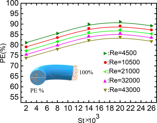
5.3.2. Effect of Dean number and Reynolds number

Figures 13 and 14 show the penetration efficiency as a function of Dean number and Reynolds number. It can be seen that the penetration efficiency decreases with increasing Dean number and Reynolds number, which is consistent with the case of spherical particles (Sato, Chen, and Pui 2003). The particles are easier to be carried toward to the walls by stronger secondary flow for the cases with larger Reynolds number and Dean number, which is different with the case for the spherical particles with large scale (0.1 μm ≤ d_p ≤ 10 μm), i.e., the penetration efficiency did not depend on either the curvature or the Reynolds number (Pui, Romay-Novas, and Liu 1987), and also different with the case with considering the inertial impaction and gravitational deposition of spherical particles, i.e., the penetration efficiency was not strongly affected by secondary flow (Balásházy, Martonen, and Hofmann 1990). The variation of penetration efficiency with Reynolds number is different from that for spherical particles with larger Stokes number. Wilson et al. (2011) showed that increasing the Reynolds number did not significantly alter the trend of penetration efficiency when St > 0.4, while resulted in a noticeable decrease in penetration efficiency for 0.1 ≤ St ≤ 0.4. For example, an increase in Reynolds number from 10,250 to 30,750 resulted in a factor of 2.6 increase in deposition fraction from 0.14 to 0.36 at St = 0.15.

Figure 13. Penetration efficiency as a function of St and De (β = 8, Re = 10,500).

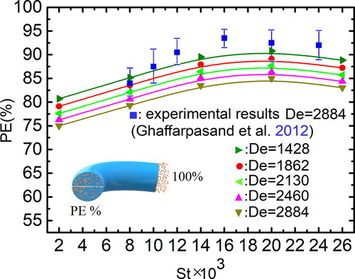
Figure 14. Penetration efficiency as a function of St and Re (β = 8, Dean = 1862).

5.3.3. Relationship of penetration efficiency and related parameters

It is necessary to build a relationship between the penetration efficiency and related parameters in order to effectively characterize the penetration efficiency. As shown in Figures 12–14, the penetration efficiency is inversely proportional to the particle aspect ratio β, Reynolds number Re, Dean Number De and Stokes number St (when St > 0.02), whereas directly proportional to the Stokes number St (when St < 0.02). So we combine β, Re, De and St into a dimensionless synthetic parameter: $$\eta =\frac{\text{St}}{\beta \text{ReDe}}\times 10^{11},\mathrm{ }\text{St}\le 0.02$$ (40) $$\eta =\frac{1}{\beta \text{ReDeSt}}\times 10^8,\mathrm{ }\text{St}\mathrm{>}0.02.$$(40)

Based on the above numerical data and expression (40(40) $$\eta =\frac{1}{\beta \text{ReDeSt}}\times 10^8,\mathrm{ }\text{St}\mathrm{>}0.02.$$(40) ), we can establish following formula of penetration efficiency PE: $$\text{PE}=77.63991+3.97688\hspace{0.17em}\text{ln}\hspace{0.17em}(\eta +0.05953),\mathrm{ }\text{St}\le 0.02$$ (41) $$\text{PE}=76.2707\mathrm{ }+\mathrm{ }3.4078\mathrm{ }\hspace{0.17em}\text{ln}\hspace{0.17em}(\eta \mathrm{–}\mathrm{ }0.0196),\mathrm{ }\text{St}\mathrm{>}0.02..$$(41)

Figure 15 shows the penetration efficiency as a function of related synthetic parameter.

Figure 15. Penetration efficiency as a function of related synthetic parameter. (a) St ≤ 0.02; (b) St > 0.02.

6. Conclusions

Distribution and penetration efficiency of cylindrical nanoparticles with length of 160 nm and aspect ratio between 2 and 16 are studied numerically in turbulent flows through a curved tube in the range of Reynolds number from 4500 to 43,000, Stokes number from 0.002 to 0.026, Dean number from 1428 to 2884. The equations of mean momentum, turbulent kinetic energy and dissipation rate, and fluctuating velocity of fluid are solved first, and then the equations of particle motion and the Fokker–Planck equations are solved to obtain the evolution and distribution of particle number concentration and particle orientation on the cross-section at different axial positions and at outlet. Based on the particle trajectories, the penetration efficiencies of particles through the curved tube are calculated. Some numerical results are compared with related experimental results. The effects of various parameters on the distributions of particle number concentration and particle orientation as well as the penetration efficiency are discussed. The research is beneficial for reducing blocking, avoiding malfunction and enhancing system efficiency. The main conclusions are summarized as follows:

The extent of non-uniformity of the distribution of particle number concentration increases with increasing Stokes number, Dean number, Reynolds number and particle aspect ratio. More particles align with their major axis near to the flow direction with the increase of the Stokes number and particle aspect ratio, than with the decrease of the Dean number and Reynolds number. The penetration efficiency increases as the Dean number, Reynolds number and particle aspect ratio decrease. However, the penetration efficiency is not a monotonic function of the Stokes number. The penetration efficiency increases and decrease with increasing Stokes number when St < 0.02 and St > 0.02, respectively. Finally, the relationship between the penetration efficiency and related synthetic parameters is established based on the numerical data.

The distribution and penetration efficiency of cylindrical nanoparticles in turbulent flows through a curved tube is a more complicated issue, and some assumptions have been made in the present study. Therefore, it is necessary to carry out related experimental research in the future.

Additional information

Funding

We would like to acknowledge the funding from National Natural Science Foundation of China (91852102).

References

- Anand, N. K., A. R. McFarland, K. D. Kihm, and F. S. Wong. 1992. Optimization of aerosol penetration through transport lines. Aerosol Sci. Technol. 16 (2):105–12. doi:10.1080/02786829208959541.
- Armand, P., D. Boulaud, M. Pourprix, and J. Vendel. 1998. Two-fluid modeling of aerosol transport in laminar and turbulent flows. J. Aerosol Sci. 29 (8):961–83. doi:10.1016/S0021-8502(98)00006-8.
- Balásházy, I., T. B. Martonen, and W. Hofmann. 1990. Inertial impaction and gravitational deposition of aerosols in curved tubes and airway bifurcations. Aerosol Sci. Technol. 13 (3):308–21. doi:10.1080/02786829008959447.
- Batchelor, G. K. 1970. Slender-body theory for particles of arbitrary cross-section in Stokes flow. J. Fluid Mech. 44 (3):419–40. doi:10.1017/S002211207000191X.
- Chen, S. B., and L. Jiang. 1999. Orientation distribution in a dilute suspension of fibers subject to simple shear flow. Phys. Fluid 11 (10):2878–90. doi:10.1063/1.870146.
- Dong, S., X. Feng, M. Salcudean, and I. Gartshore. 2003. Concentration of pulp fibers in 3D turbulent channel flow. Int. J. Multiphase Flow 29 (1):1–21. doi:10.1016/S0301-9322(02)00128-3.
- Fung, J. C. H., J. C. R. Hunt, N. A. Malik, and R. J. Perkins. 1992. Kinematic simulation of homogeneous turbulence by unsteady random Flourier modes. J. Fluid Mech. 236:281–318. doi:10.1017/S0022112092001423.
- Ghaffarpasand, O., F. Drewnick, F. Hosseiniebalam, S. Gallavardin, J. Fachinger, S. Hassanzadeh, and S. Borrmann. 2012. Penetration efficiency of nanometer-sized aerosol particles in tubes under turbulent flow conditions. J. Aerosol Sci. 50:11–25. doi:10.1016/j.jaerosci.2012.03.002.
- Krushkal, E. M., and I. Gallily. 1988. On the orientation distribution function of non-spherical aerosol particles in a general shear flow-ii. the turbulent case. J. Aerosol Sci. 19 (2):197–211. 8502(88)90223-6. doi:10.1016/0021-.
- Launder, B. E. 1989a. Second-moment closure and its use in modeling turbulent industrial flows. Int. J. Numer. Methods Fluids 9 (8):963–85. doi:10.1002/fld.1650090806.
- Launder, B. E. 1989b. Second-moment closure: Present and future? Int. J. Heat Fluid Flow 10 (4):282–300. doi:10.1016/0142-727X(89)90017-9.
- Leal, L. G., and E. J. Hinch. 1971. Effect of weak Brownian rotations on particles in shear flow. J. Fluid Mech. 46 (4):685–703. doi:10.1017/S0022112071000788.
- Lee, K. W., and J. A. Gieseke. 1994. Deposition of particles in turbulent flow pipes. J. Aerosol Sci. 25 (4):699–704. doi:10.1016/0021-8502(94)90011-6.
- Lien, F. S., and M. A. Leschziner. 1994. Assessment of turbulent-transport models including non-linear RNG eddy-viscosity formulation and second-moment closure. Comput. Fluids 23 (8):983–1004. doi:10.1016/0045-7930(94)90001-9.
- Lin, J. Z., L. J. Qian, H. B. Xiong, and T. L. Chan. 2009. Effects of operating conditions on droplet deposition onto surface of atomization impinging spray. Surf. Coat. Technol. 203 (12):1733–40. doi:10.1016/j.surfcoat.2009.01.009.
- Lin, J. Z., L. X. Zhang, and W. F. Zhang. 2006. Rheological behavior of fiber suspensions in a turbulent channel flow. J. Colloid Interface Sci. 296 (2):721–8. doi:10.1016/j.jcis.2005.09.038.
- Lin, J. Z., P. F. Lin, and H. J. Chen. 2009. Research on the transport and deposition of nanoparticles in a rotating curved pipe. Phys. Fluids 21 (12):122001. doi:10.1063/1.3264110.
- Lin, J. Z., Z. Q. Yin, F. J. Gan, and M. Z. Yu. 2014. Penetration efficiency and distribution of aerosol particles in turbulent pipe flow undergoing coagulation and breakage. Int. J. Multiphase Flow 61:28–36. doi:10.1016/j.ijmultiphaseflow.2013.12.001.
- Lin, J. Z., Z. Q. Yin, P. F. Lin, M. Z. Yu, and X. K. Ku. 2015. Distribution and penetration efficiency of nanoparticles between 8–550 nm in pipe bends under laminar and turbulent flow conditions. Int. J. Heat Mass Transf. 85:61–70. doi:10.1016/j.ijheatmasstransfer.2015.01.033.
- Mackaplow, M. B., and E. S. G. Shaqfeh. 1998. A numerical study of the sedimentation of fiber suspension. J. Fluid Mech. 376:149–82. doi:10.1017/S0022112098002663.
- Matsusaka, S. 2015. High-resolution analysis of particle deposition and resuspension in turbulent channel flow. Aerosol Sci. Technol. 49 (9):739–46. doi:10.1080/02786826.2015.1066752.
- Michaelides, E. E. 2015. Brownian movement and thermophoresis of nanoparticles in liquids. Int. J. Heat Mass Transf. 81:179–87. doi:10.1016/j.ijheatmasstransfer.2014.10.019.
- Muyshondt, A., N. K. Anand, and A. R. McFarland. 1996. Turbulent deposition of aerosol particles in large transport tubes. Aerosol Sci. Technol. 24 (2):107–16. doi:10.1080/02786829608965356.
- Peters, T. M., and D. Leith. 2004. Particle deposition in industrial duct bends. Ann. Occup. Hyg. 48:483–90. doi:10.1093/annhyg/meh031.
- Phares, D. J., and G. Sharma. 2006. A DNS Study of aerosol deposition in a turbulent square duct flow. Aerosol Sci. Technol. 40 (11):1016–24. doi:10.1080/02786820600919416.
- Podgórski, A., L. Gradoń, and P. Grzybowski. 1995. Theoretical-study on deposition of flexible and stiff fibrous aerosol-particles on a cylindrical collector. Chem. Eng. J. 58 (2):109–21. doi:10.1016/0923-0467(95)02975-3.
- Pui, D. Y. H., F. Romay-Novas, and B. Y. H. Liu. 1987. Experimental study of particle deposition in bends of circular cross section. Aerosol Sci. Technol. 7 (3):301–15. doi:10.1080/02786828708959166.
- Quek, T. Y., C. H. Wang, and M. B. Ray. 2005. Dilute gas-solid flows in horizontal and vertical bends. Ind. Eng. Chem. Res. 44 (7):2301–15. doi:10.1021/ie040123i.
- Sato, S., D. R. Chen, and D. Y. H. Pui. 2003. Particle transport at low pressure: Deposition in bends of a circular cross-section. Aerosol Sci. Technol. 37 (10):770–9. doi:10.1080/02786820300911.
- Shapiro, M., and M. Goldenberg. 1993. Deposition of glass-fiber particles from turbulent air-flow in a tube. J. Aerosol Sci 24 (1):65–87. doi:10.1016/0021-8502(93)90085-N.
- Sturm, R. 2015. A computer model for the simulation of nanoparticle deposition in the alveolar structures of the human lungs. Ann. Transl. Med. 3 (19):281. doi:10.3978/j.issn.2305-5839.2015.11.01.
- Sun, K., L. Lu, H. Jiang, and H. H. Jin. 2013. Experimental study of solid particle deposition in 90 degrees ventilated bends of rectangular cross section with turbulent flow. Aerosol Sci. Technol. 47 (2):115–24. doi:10.1080/02786826.2012.731094.
- Tsai, C. J., and D. Y. H. Pui. 1990. Numerical study of particle deposition in bends of a circular cross-section- laminar flow regime. Aerosol Sci. Technol. 12 (4):813–31. doi:10.1080/02786829008959395.
- Wang, J., R. C. Flagan, and J. H. Seinfeld. 2002. Diffusional losses in particle sampling systems containing bends and elbows. J. Aerosol Sci. 33 (6):843–57. doi:10.1016/S0021-8502(02)00042-3.
- Wang, L. P., and D. E. Stock. 1994. Numerical simulation of heavy particle dispersion-scale ration and flow decay considerations. J. Fluids. Eng. Trans. ASME 114 (1):100–6. doi:10.1115/1.2909983.
- Webster, D. R., and J. A. C. Humphrey. 1993. Experimental observations of flow instability in a helical coil. ASME J. Fluids Eng. 115 (3):436–43. doi:10.1115/1.2910157.
- Wilson, S. R., Y. A. Liu, E. A. Matida, and M. R. Johnson. 2011. Aerosol deposition measurements as a function of Reynolds number for turbulent flow in a ninety-degree pipe bend. Aerosol Sci. Technol. 45 (3):364–75. doi:10.1080/02786826.2010.538092.
- Yook, S. J., and D. Y. H. Pui. 2006. Experimental study of nanoparticle penetration efficiency through coils of circular cross-sections. Aerosol Sci. Technol. 40 (6):456–62. doi:10.1080/02786820600660895.