Droplet and particle methods to investigate turbulent particle laden jets

Abstract

The SARS-CoV-2 pandemic has heightened the interest in particle-laden turbulent jets generated by breathing, talking, coughing and sneezing, and how these can contribute to disease transmission. We present quantitative measurement methods for such flows, while exploring and offering improvements for common shortcomings. We generate jets consisting of either liquid droplets or solid particles in an isothermal, quiescent and electrically isopotential experimental chamber that was constructed to control the effects of ambient forcing on jet behavior. For liquid droplets, we find promise in surface deposition analysis based on fluorescent tracer use. For particles, we explore the performance of commercially available adhesive sampling strips and develop conductive grounded carbon tape based sampling strips. We explore ways in which the smallest of thermal gradients or electrostatic charge issues can affect particle dispersion, and suggest practical methods to address these issues. The developed methods are applied to study the simultaneous deposition of $\approx$ 25, 50 and 200 μm solid particles from a particle laden turbulent jet with a mean velocity of 33.2 m/s. The deposition location as a function of particle size was compared to results from a simple numerical RANS model, and illustrates ways in which imprecise initial or boundary conditions can lead to a notable deviation from experimental results. The differences in deposition pattern seen in experimental and numerical results despite a carefully controlled environment and characterized particle ejection indicate the need for a more stringent numerical model validation, especially when studying fate and transport of mid-range (neither purely aerosol or ballistic) sized particles.

EDITOR:

• Jing Wang

1. Introduction

A major vector of coronavirus is thought to be respiratory droplets that are expelled when coughing, speaking, and breathing (e.g., Bahl et al. 2020). To reduce person-to-person exposures, we are seeing businesses, schools, and other building owners implement safety measures that could minimize the risk of exposure to the coronavirus. Approaches to testing the efficacy of the mitigation measures are often empirical and range widely in their thoroughness. These shortcomings serve to highlight the importance of understanding respiratory aerosol transport from first principles.

Numerous measurements have addressed the question of droplet and aerosol transport in practical environments. The articles published in recent months present a wide spectrum of qualitative and quantitative data, for which several reviews exist (e.g., Jayaweera et al. 2020; Kohanski, Lo, and Waring 2020; Bahl et al. 2020; Chu et al. 2020). Of particular interest is the transport of respiratory aerosols in medical facilities, using, e.g., benign bacteriophages (Sze To et al. 2008), liquid droplets (Wan et al. 2007; Qian and Li 2010; Lindsley et al. 2012), or the SARS–COV2 virus itself (e.g., Nissen et al. 2020). Additional papers on practical environments include the movement of aerosols in an airline cabin (Zhang, Chen, et al. 2009), laboratory (Liu et al. 2020), furnished office–type space (Richmond-Bryant et al. 2006) or multi–zone indoor spaces (Miller and Nazaroff 2001).

Measurements in practical environments cannot provide all of the boundary conditions needed to validate numerical models. Thus some measurements have used controlled environmental chambers to study aerosol motion. These can include the influence of common sources of convection such as thermal plumes, ventilation, or air conditioning (Zhang and Chen 2006; Murakami 1992; Liu and Novoselac 2014; Lai and Wong 2010; Chao and Wan 2006; Jurelionis et al. 2015; Jin et al. 2009; Bolster and Linden 2009; Seepana and Lai 2012). These can also focus on the fundamental case of respiratory jets with nominally no background flow (Wei and Li 2017; Zhu, Kato, and Yang 2006; Bourouiba, Dehandschoewercker, and Bush 2014; Bourouiba 2016; Lee et al. 2019). The work discussed here is of the latter type, focusing on jets with no background flow.

Though there is still much more to learn, many researchers have pursued measurements in nominally quiescent environments in recent years. Droplet production and transport from a sneeze was investigated in Bourouiba (2016) and Bourouiba, Dehandschoewercker, and Bush (2014). Comparing sneeze flows to measured fallout and deposition from a particle–laden multi–phase puff in a water tank, they created a theoretical model to predict droplet transport distance. Also using a water tank, Wei and Li (2017) show the importance of how the temporal variation in flowrate impacts the transport patterns in a simulated cough. The approach of using water tanks and applying similitude to translate the results to air is a practical way to simplify some of the challenges of working with real aerosols (discussed below). Still, there are limits to what can be achieved with similitude, given that particles are typically O(1)–O(10) times denser than water while particles and droplets are typically O(1000) times denser than air. Therefore there is a need to directly measure aerosol transport in air.

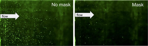
A major challenge in directly measuring respiratory aerosols is managing their broad size distribution. Optical measurements must correct for the nonlinear effects of scattering, which becomes challenging when the optical path between emitter and receiver is complex. For example, laser–sheet imaging (shown from our laboratory in Figure 1) produces results that are biased toward large particles in a manner that is very difficult to correct. This bias is important for the work of Zhu, Kato, and Yang (2006), who used particle image velocimetry (PIV) to measure cough–ejected particles using three healthy male subjects. Bourouiba, Dehandschoewercker, and Bush (2014) note the size–selectivity of optical methods in their quote, “more droplets and mist were observed with naked eye than the camera.” In our experiments (discussed below) there were also biases in the optical methods found within some optical particle counters (OPCs). These biases may affect the work of Zhang et al. (2009) which measures the dispersal of nanoparticle aggregates using multiple optical particle counters within a room. Some measurement methods that manage the difficulties of particle or droplet size distribution are discussed later in this article.

Figure 1. Light–sheet imaging of respiratory jets from a speaking person with and without a surgical mask (field of view 50 cm wide). The axis and direction of the jet are indicated by the arrow and are opposite to those of the laser light sheet. The imaging misses many of the smaller droplets in a way that is greatly affected by laser quality, image–capture settings, optical components and their alignment.

Quantified background flows contribute greatly to the value of idealized experiments. Discussion of these flows varies from qualitative to quantitative. On the qualitative side, Jones and Nicas (2009) described the background thermal convection visible when using fluorescein–dyed liquid droplets to measure deposition patterns in a nominally quiescent room. Sajo, Zhu, and Courtney (2002) extended this conclusion by discussing how deviations between the measured and modeled deposition of 0.01–15 μm solid particles on adhesive collector foils may have been caused by thermal gradients or electrostatic effects. Lee et al. (2019) quantify the background flow inside their study space using the metric of air changes per hour (ACH) and report ACH = 0.0037–0.0056 for their measurement of respiratory aerosols in a cleanroom.

The particle size range considered by previous researchers leaves some gaps to be filled. Respiratory aerosols are known to span the range of $<1\hspace{0.5em}\mu m$ to $<100\hspace{0.5em}\mu m$ (Tang et al. 2021). However, Jones and Nicas (2014) notes the lack of room–scale validation–quality experiments with particles larger than 1 micron. This is of particular concern because the 1–100 micron range includes a changeover from tracer behavior to motion dominated by particle momentum and gravitational settling (Hinds 1999). This size range is also especially important when considering liquid droplets: as reported in Wang, Wu, and Wan (2020) mid–range ($\approx 50\mu m$) droplets are especially sensitive to the rate of evaporation. Furthermore, mid range sized droplets are poorly covered by the popular discrete random walk (DRW) models (Wei and Li 2015).

Having reviewed these previous works, we conclude that more attention is needed in several areas: (1) decreasing the effect of boundary conditions on particle and droplet deposition measurements; (2) measuring the transport of particles and droplets from 1–100 μm; and (3) sampling particles and droplets in a manner that captures the size distribution accurately. We address these three issues herein and present some timely data on droplet and particle transport by a turbulent jet in an environment with carefully controlled boundary conditions. We achieve this using a variety of techniques (high–speed imaging and charge–neutral deposition sampling) and discuss others that we ruled out along the way. The methods laid out in this work address key challenges in producing steady, uniform, and accurately measured boundary conditions in particle and droplet transport experiments.

The article is organized as follows: Section 2 provides a brief review of the relevant physical phenomena. Section 3 discusses the laboratory facility we constructed for controlling boundary conditions. Section 4 discusses methods for droplet measurement and Section 5 discusses methods for particle measurement. Section 6 presents data for a canonical turbulent jet loaded with particles in a carefully controlled environment. Section 7 compares this data with results from a widely implemented CFD model. Raw experimental data suitable for CFD validation is included in the Appendix.

2. Background

Droplets and particles can be considered as different categories based on their composition or their surface slip behavior. While some works refer to both generically as ‘particles,’ in this work a clear distinction is made. We use the term ‘particle’ to describe those objects that begin their journey from the jet as a solid. We use the term ‘droplet’ to describe objects that are initially fluid, although it is important to note that the liquid can evaporate and effectively transform the droplet into solid particles composed of non–evaporative material.

Droplets and particles can also be categorized based on their dynamics, e.g., by their Stokes number or the continuum from ‘aerosol’ to ‘ballistic’ behavior. An aerosol quickly loses its initial momentum, settles slowly through the local flow over minutes (or hours), and is generally a faithful flow tracer. A ballistic particle or droplet maintains its initial momentum long enough to significantly cross streamlines, and thus mostly follows its own trajectory. We can use projectile motion equations to estimate time for a ballistic particle to reach ground $t_{\mathit{fall}}\approx \sqrt{(2h/g)},$ where h is the initial height and g the acceleration due to gravity. Thus a ballistic particle starting at a human nose 165 cm high will settle to the floor in $\approx 0.6$ sec. Herein we consider particles that are in between the extremes of ballistic and aerosol dynamics. These ‘mid–range’ droplets and particles have diameters 1–100 μm. Their trajectory is a strong function of both their initial momentum and the local flow field.

In the ‘mid–range,’ there is not a completely closed equation for momentum conservation on a particle or droplet approximated as a single point mass. Terms related to finite–size and unsteady effects are discussed in Guazzelli and Morris (2011). A greatly simplified version, keeping only the first–order terms in added mass, drag, buoyancy, and electrophoresis is: (1) $$(m+\frac{1}{2}{m}_f)\ddot{\mathbf{x}}=\frac{1}{2}{\rho }_f{C}_d\left(\pi \frac{d^2}{4}\right)\left|\right|{\dot{\mathbf{x}}}_f-\dot{\mathbf{x}}\left|\right|({\dot{\mathbf{x}}}_f-\dot{\mathbf{x}})+(m-m_f)\mathbf{g}+q\mathbf{E}(\mathbf{x})$$(1) where m is particle mass, m_f is the mass of displaced fluid, $\ddot{\mathbf{x}}$ is the particle acceleration, $\dot{\mathbf{x}}$ is the particle velocity, ${\dot{\mathbf{x}}}_f$ is the fluid velocity, C_d is the Reynolds–number–dependent drag coefficient, d is the particle diameter, g is the gravitational acceleration, q is the charge of the particle, and E the electric field experienced by the particle. This equation is the starting point for many numerical simulations of particle–laden turbulent jets (e.g., Zohdi 2020). Clever modifications are needed to extend the point–mass formulation to one that includes effects such as evaporation, condensation, (dis)aggregation, and reaction. These extended models enable practical engineering solutions, and thus deserve careful validation. Data useful for such validation is the focus of the work presented below.

The presence of particles or droplets in a flow can radically change the flow dynamics, notably the turbulence. One classification scheme names this effect “two–way coupling,” in contrast to the “one–way coupling” regime in which the fluid flow is not significantly modified by the presence of suspended material. The particle–laden jet can be in either regime depending on the concentration and properties of particles or droplets. Particle–laden jets have been studied in many contexts, from internal combustion to environmental processes (e.g., Bordoloi et al. 2020).

From these studies, we know that the droplet– or particle–laden jet is affected by ambient temperature gradients (e.g., Jones and Nicas 2009), radiative forcing (e.g., Stan et al. 2016), relative humidity, contaminants, pressure waves, and of course forced and natural convection. The ‘near–field’ motion is dominated by the jet orifice, mass flowrate, and momentum flowrate. The ‘far–field’ motion is more strongly influenced by instabilities and turbulence in the jet, as well as the ambient features listed above. The next section describes our attempt to control ambient conditions well enough to achieve repeatable deposition measurements.

3. Laboratory facility

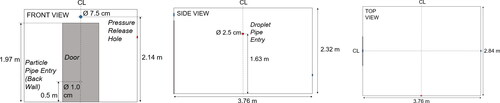
The Cal Covid Cube, C³, was set up to evaluate experimental methods and provide data suitable for validating numerical models. The C³ is a parallelepiped room that is 232 cm tall, 376 cm long, and 284 cm wide on the inside. A diagram of the C³ is included in Figure 2. The three main features of the C³ are as follows:

Figure 2. Inside dimensions of C³ including pipe entry and pressure release holes. During particle release the droplet pipe entry hole was closed and vice versa. During all experiments the door was closed.

• Isothermal. The C³ has 10.5–13 cm of thermal insulation surrounding it on all sides, built using the methods from walk–in freezers. The C³ is located in the middle of a building at least 5 m away from all building walls, with no direct sunlight exposure. All building air supplies within 3 m of the C³ are disabled; when these supplies were not blocked, a temperature gradient $(\approx {0.4}^{°}C)$ developed across the interior of the C³ and led to a detectable convective flow inside the C³. The ceiling is also insulated, with both foam and a 21–cm air gap between the interior and exterior surfaces. The insulated floor rests on a concrete floor. An empty sub–basement is beneath the floor, helping shield the floor from daily variation in temperature. Temperature uniformity was checked with an Extech 42542 infrared (IR) thermometer (nominal uncertainty $\pm 2^{°}C$) and two Hobo MX2302A data loggers (nominal uncertainty $\pm {0.2}^{°}C$). Before each measurement of a particle–laden jet, we confirmed that temperatures were isothermal within the uncertainty of these thermometers.

• Quiescent. The isothermal conditions discussed above keep the thermal convection in the C³ to a minimum. Flows driven by external pressure gradients are also non-detectable (and presumed negligible) because there are only two access holes connecting the exterior and interior of the C³. The first access hole supplies the jet via a pipe of inner diameter 9.78 ± 0.02 mm) tightly fitted through the hole. The second hole (diameter 75 mm) is to release pressure from the C³ as the jet delivers air. It is located directly across from the jet orifice, but higher up the wall (see Figure 2). That is, the pressure release hole is at a height of 213.5 cm while the jet is at a height of 50.2 ± 0.2 cm. Quiescence was verified with both hot wire measurements and with the particle–deposition measurements described at length below. In these, free–falling particles $O(30 \mu m)$ showed the same deposition pattern with no observable drift in many repeated observations.

• Isopotential. Accumulated charge on the C³ can significantly change the deposition pattern of particles and drops, as discussed further below. To prevent this, the outer and inner surfaces of the C³, including all parts of the door, are finished with conductive material (conductive aluminum and stainless steel) and connected to each other with copper tape. The door, interior shell, and exterior shell were tied to building ground. Inspection for electrical path resistance revealed no measurable resistance within the accuracy of the Fluke 87V multi-meter. Electric fields were surveyed with Simco–Ion FMX–003 electrostatic field meter and found to be negligible within precision of instrument (±0.1 kV).

Other design elements include an all–matte–black interior to support imaging and also a location on the ground floor to limit vibrations.

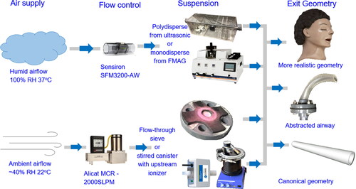
Figure 3 shows the system designed to repeatably release both solid particles and droplets in a jet. The air in the jet can be set humid or dry, and the jet exit can be canonical (fully developed with a circular cross–section) or a geometry based on the human airway. We call this system the “Repeatable Respirator Rig” (R³).

Figure 3. Schematic of the Repeatable Respirator Rig, R³. Note that the particle trap is shown uncovered in this figure.

Repeatability was our goal, even though cough and sneeze flows are unique to the individual (see Yang et al. 2007) with variable velocities and droplet densities. We simplify the release by considering different layers of complexity that take us from a canonical turbulent jet toward a true cough or sneeze. To do this we consider the following three jet orifices, in order of increasing complexity (Figure 4):

Figure 4. Snapshot of particle ejection from (a) straight pipe, (b) smooth ${90}^{°}$ curved pipe, (c) intubation trainer doll, with realistic airways and mouth/tongue structure.

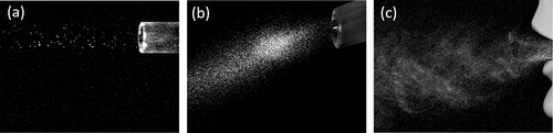
1. Straight round pipe with sufficient length to reach fully developed flow.

2. Smooth ${90}^{°}$ curved pipe, with a changing radius along the length of the pipe.

3. Intubation trainer doll, with realistic airways and mouth/tongue structure.

Jet exit conditions are measured differently for droplets and particles. For the latter, particle tracking velocimetry (PTV) was used and is presented in Section 6. For droplets, a phase Doppler interferometer on a 3–axis traverse was used and data from this will be included in a subsequent publication.

4. Droplet measurements

The free exchange of mass across the air-liquid interface introduces significant complexity in the study of droplets. Droplets can grow or shrink as a result, and this occurs at timescales short enough that initial conditions alone are likely insufficient to predict droplet transport. In other words, the boundary conditions are of key importance. This is true for both the air– and liquid–phases. In both phases, the rate of cross–interface exchange is set by temperature, solutes, and flow patterns. A notable example is the presence of salt in water droplets. Saltwater droplets can reach an equilibrium size under the same conditions for which pure water droplets evaporate entirely.

The humidity and temperature of the co-flowing air affect the size of droplets via evaporation or condensation. The temperature of the co-flowing air also can add to the buoyancy difference between the droplet–laden jet and the ambient air into which it flows. Even if the co-flowing air begins at the same temperature and humidity as the ambient air, it can become cooled if droplets are evaporating.

To prevent premature changes in droplet size, we designed a system to provide co-flowing air at nearly 100% relative humidity (RH). We chose to heat the co-flow to 37${}^{°}$ C to match the typical temperature of human respiratory exhalations. To achieve this, we pull air over a reservoir of water heated to 40${}^{°}$ C. The reservoir is the famous “Einstein flume” in which Hans Albert Einstein measured fluvial sediment transport (Einstein and Shen 1964). After traveling along the flume for 16.9 m, the RH and temperature were measured and the air injected with droplets. Humidifying in this way is preferable to adding droplets intended to evaporate, because it ensures that the only droplets are those that we intend to study.

Liquid droplets were generated using either (i) an ultrasonic transducer in a constant–depth water bath generating polydisperse droplets or (ii) a flow–focusing aerosol generator producing nominally monodisperse droplets (TSI model 1520). In both cases the droplets are made by mechanical means from water with a controlled amount of fluorescent dye (Sigma-Aldrich Fluorescein sodium salt F6377).

The humid droplet–laden flow was fed to a pipe, and at the exit of the pipe a phase Doppler interferometer measures droplet size and velocity. In this study, a straight pipe with $2.38\pm 0.005$ cm diameter and $117\pm 1$ cm length (L/D = 49) was utilized to simplify the initial condition (i.e., to have a nominally fully developed pipe flow at the exit). A subsequent publication incorporates additional launch methods as well as the discussion on plume buoyancy effects.

Deposition of droplets on the floor was quantified by collecting drops in plastic weigh boats on a horizontal grid. The C³ door was not opened until 30 min after the experiment to ensure that droplets >$3.6 \mu m$ had settled. A standard amount of water, in this case 3 mL, is added to each weigh boat to collect the deposited dye. The concentration of dye in this water is measured using a fluorometer (Turner instruments 10 AU) with a minimum detection limit of 0.01 ppb. It uses a 510–700 nm emission filter and a narrowband 491 nm excitation filter designed specifically for detecting fluorescein. A calibration was conducted with an average error of 3% for a given measurement over a range of 0.05 ppb to 240 ppb Fluorescein.

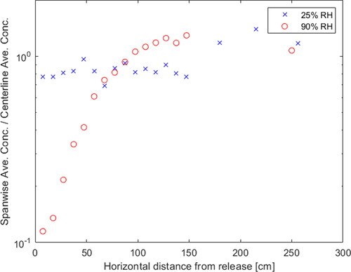
While a companion article is being prepared with full results, we report here the difference between identical droplet–laden jets entering ambient air with 90% vs. 25% relative humidity. As seen in Figure 5, in the low–humidity environment droplets spread much more evenly throughout the room. This is likely due to faster evaporation in a drier environment, leading to smaller droplets. The higher residence time of these droplets allows for more even dispersal by convection from the flow set up in the C³ by the droplet-laden jet. The effects of humidity on droplet size are explored further in Yang and Marr (2011).

Figure 5. Initial experiments of droplet deposition measured by the fluorescein method. Ambient air is at T = 22${}^{°}$C and 90% relative humidity. The source of the jet was located at a height of 163 ± 1 cm, and measurements were made on the floor of the C³. Plotted concentrations are normalized by the average concentration along the centerline of droplet ejection.

5. Methods for (and problems with) particles

Using solid particles (e.g., plastic microbeads) removes the effect of evaporation that makes droplet studies difficult. It is also possible to use different colored particles, corresponding to tightly controlled sizes, to track size effects. Herein we use Cospheric fluorescent polyethylene microspheres.

5.1. Particle launch

For data presented here, particles are released at steady state in fully–developed pipe flow, from an $L/D=88$ straight pipe with circular cross–section. This provides a simpler case for numerical model validation than the releases that are more relevant to respiratory aerosols, e.g., unsteady emissions from models that approach the complexity of human anatomy (see Figure 3). Data from more complex cases are presented in a companion article.

The particle–laden pipe–flow sets the initial conditions for the jet (Picano, Sardina, and Casciola 2009). We work in the regime for which (a) gravitational settling within the pipe is negligible and (b) the number density of particles is small enough that flow can be assumed one–way coupled. Uniform particle distribution across the pipe at exit was confirmed with high–speed video of particles. These videos also confirmed that there was no saltation or rolling of particles along the bottom of the pipe. To reach this flow regime, we use a flow rate of 149.6 ± 2.4 slpm so that the average velocity is 33.2 ± 0.6 m/s in a pipe with diameter 9.78 ± 0.02 mm. Thus, the pipe–flow Reynolds number was $\approx 21,500.$

Particle releases that are near–instantaneous were achieved using a custom “particle trap” in which the starting–jet flow moves vertically through a mesh on which particles are suspended, picking them up and pushing them out of the pipe. Steady–state particle releases were achieved using the LaVision GMBH “Particle Blaster” which is a stirred canister in which the particles are kept suspended by the flow–through–induced circulation in the cavity. A magnetic stir bar is also available to agitate the contents of the cavity, but was not used because it shattered some of the particles.

Measurements of particle transport will be disrupted if the particles aggregate or gather charge. We prevent aggregation by using particles large enough that the attraction due to surfactants or by Van der Waals Forces has minor effects. To eliminate particle tribocharging, two in-line air ionizers (Simco-Ion 4210 u) are placed in series prior to air injection into the particle blaster, the ceramic inside of the particle blaster was lined with copper, tubing from blaster to pipe was minimized and grounded metallic tubing was used where possible.

The lack of aggregation was confirmed at the jet exit by high–speed imaging (without the charge–neutralizing ionizer) and in the sample strips discussed in the next section (both with and without charge neutralization). The lack of particle charging was confirmed by examining particle deflection on sampling strips charged to $\approx 7$ kV, discussed further below.

5.2. Particle collection

Our methods focused on quantifying surface deposition. In–air sampling by optical particle sensors (OPS’s) was also tested, but there were several challenges that led us to focus on deposition instead. Typical optical particle counters (OPCs) are designed for small particles. The OPS designed to measure particle of the size we used (22–212 μm) could not robustly separate and size the well–characterized particles used in our tests. This is likely due to the high concentrations of background particles (many devices are designed for use in clean–rooms). Upgrading these devices to utilize more of the color spectra would help, as is done in devices which identify particulate matter that comes from combustion.

Passive collection (deposition) has been done on glass, foil, silicon “witness wafers,” and adhesive “coupons” or “strips.” Active collection pulls air through a filter that is later washed to collect the particles; this method can amplify the signal by increasing the “footprint” of the sample. We chose to use passive collection and developed two methods that unite the benefits of foil and adhesive sampling. Adhesive sampling allows users to move and store the samples without risk of disturbing the particles, but care must be taken to ensure the strip does not retain a static charge. Foil sampling allows the surface to be charge–neutralized. The two methods are: (1) grounded aluminum–backed carbon sampling strips, (2) non–conductive adhesive sampling strips (TriTech vinyl backed print lifters) treated with an ionizer. Strips are set out on the ground in a grid below the jet outlet. A surface concentration is calculated for each strip by optical imaging.

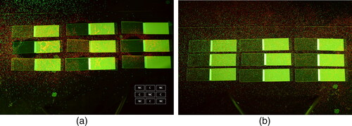
Static charge effects can manifest through particle–particle or particle–surface interaction, both of which affect particle deposition patterns. The effect of neutralizing sampling strips with an ionizer is seen in Figure 7. The process of peeling off the cover to expose adhesive charges the sampling strips, and this repels particles as seen in subplot (a). Neutralized strips do not repel particles, as seen in subplot (b). The non–conductive sampling strips were ionized by placing them underneath a Simco–Ion 5225 AeroBar until the static charge (measured with Simco–Ion FMX–003 electrostatic fieldmeter) on the strip was between $[-0.2kV,+0.2kV].$ This was an empirical limit for charge below which there was no noticeable difference in deposition between the sampling strip and the charge–neutralized floor. The conductive adhesive strips (carbon tape with aluminum backing) were grounded to the isopotential C³ floor and walls.

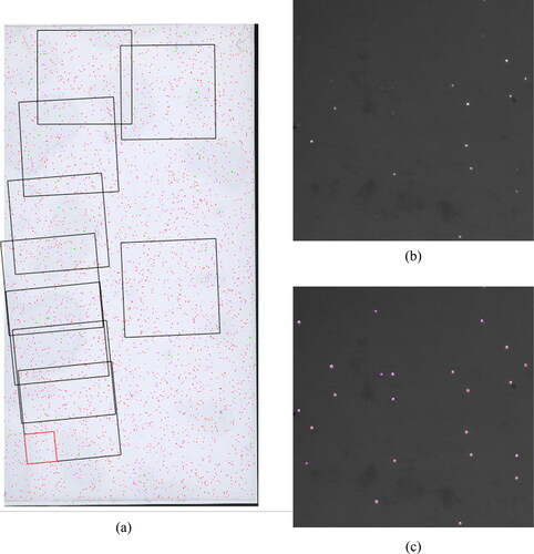
To image the particles on a sample strip we tried research–grade slide–scanning microscopes, scientific digital cameras with macro–lenses, teaching–grade USB microscopes, and finally found the best balance of speed and quality with a commercial flat–bed scanner. We pushed the detection limit of this method by working at 6400 dot–per–inch scans and post–processing using the Hough transform to identify particles in the target size range. Accuracy of particle counts was improved with layered checks using color intensity and particle shape for the rejection of crushed/broken particles, dust/debris, and other foreign bodies. With these efforts, we were able to measure particles of 20 μm and larger.

To verify accuracy of the particle–counting code, a comparison of 22–27 μm particle counts from the scanned image was made to images taken with Zeiss AxioZoom microscope with 7.0x objective and mCherry bandpass filter, for which results are seen in Figure 6. Over the imaged area of the sample strip (48.0% of total, when accounting for overlap in microscope images), there are 1080 matched red particles, 18 unmatched red particles, and 18 false positives. This amounts to a matching rate of 98.4% and a false positive rate of 1.6%. Violet particles were matched based on position but since the microscope images were monochrome a separate count of missed violet particles was not possible. Notably this error is significantly below the variation in particle count seen from test to test (a full listing of the test–to–test variation across locations and particle sizes is provided in Table 4). A research team with extensive microscopy resources could likely extend our method to smaller particles. However, this would also require interventions in particle aggregation such as delivering particles from a fluidized bed.

Figure 6. (a) Locations of microscope images superimposed on particle scan with identified particles. Red highlighted section indicates location of (b) microscope image of strip with red bandpass filter applied. (c) Particle counting comparison where red circle indicates match of 22–27 μm particle and violet circle indicates match of 45–53 μm particle.

5.3. Analyzing charge effects

It should be noted that had the particles not been fluorescent and large enough to be imaged with a wide field of view (encompassing the sampling strips), charge effects would not have been readily observable. To determine if electrophoresis can be neglected in the more general case, the force resulting from an external electric field on a charged particle could be compared to the force of gravity or drag force. (2) $$F_{\mathit{electrophoresis}}=q_{\mathit{particle}}E$$(2) (3) $$F_{\mathit{drag}}=\frac{1}{2}{\rho }_f{C}_d\left(\pi \frac{d^2}{4}\right)\left|\right|{\dot{\mathbf{x}}}_f-\dot{\mathbf{x}}\left|\right|({\dot{\mathbf{x}}}_f-\dot{\mathbf{x}})$$(3) (4) $$F_{\mathit{gravity}}=(m-m_f)\mathbf{g}$$(4)

When $F_{\mathit{electrophoresis}}\ll F_{\mathit{gravity},\mathit{drag}}$ we assume the former is negligible. However, no common criteria appears to be evoked in most cases when assuming this negligible.

To estimate the charge on particles due to tribocharging, the work of Taghavivand et al. (2021) can offer a starting point. Discussion by Matsuyama (2018) on the theoretical maximum charge a given particle can acquire, as a function of material properties and particle size, may be another practical way to evaluate the potential importance of charge effects.

Even without evaluating particle charge one can make scaling arguments on the effect of charge interventions. For example, a reduction in sampling strip charge from $\approx 7$ kV to 0.2 kV is expected to reduce the magnitude of the electric field, $E=\frac{dV}{dx},$ by a factor of $\approx 35.$ This reduction is expected to reduce the size of ‘halos’ (see Figure 7) on the sampling strips into which no particles were deposited from 1.1x the strip width to 0.03x the strip width, or to be practically negligible.

Figure 7. (a) Comparison of particle deposition on alternating charged (C) and neutralized (NC) strips with no effort to eliminate particle tribocharging. (b) Deposition on the same pattern of strips with particle tribocharging eliminated upstream of the jet.

Charge can of course also affect particle-particle interaction, in particular if one has dense particle laden flows. Elghobashi (1994) (with recently proposed updates Elgobashi 2006) offers an approximate criteria for when the flow could be considered one-way coupled due to turbulence considerations. In this dilute regime, particle to fluid and particle-particle interactions can be neglected. In the present work the average particle volume fraction in the jet is well below $1\times {10}^{-6},$ the limit below which particle-particle interaction is assumed negligible. However, during initial particle ejection (in which particle density is higher) the interventions to reduce particle tribocharging provide additional rationale for neglecting particle-particle charge effects despite uncertainty in the local instantaneous volume fraction.

6. Particle–laden jet results

For experiments in the isothermal, quiescent environment, we have the following inlet and boundary condition data: (1) Velocity at jet orifice obtained via high–speed video; (2) Temperature for all four walls, ceiling, and floor; (3) Air temperature and RH at two corners of the C³ interior. Having set these conditions, we measure particle deposition at 35 sites on the floor, using three different particle sizes simultaneously. As discussed above, the jet and sampling strips have been charge–neutralized to remove biases in sampling. The jet discussed herein is from the steady–state flow through a fully–developed circular pipe; other jets (see Figure 3) are discussed in a companion article.

In this set of experiments, a flow rate of 149.6 ± 2.4 slpm flows through a pipe with diameter 9.78 ± 0.02 mm (L/D = 88) for 30 s, producing a steady-state jet with an average velocity of 33.2 ± 0.6 m/s. The flow rate reached 90% of the maximum flow rate in 0.6 s. Analyzing high speed video footage of the first 9.44 s of flow from the pipe, we saw that 90.4% of 180–212 μm particles were ejected after steady–state flow is reached. Thus we conclude that over 90% of the total particle mass was released at steady–state.

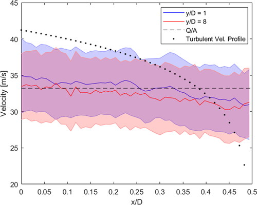
Given the significant development length for the turbulent jet, the fluid was expected to be ejected in a top–hat velocity profile with nominal velocity of $V=V_{\mathit{ave}}=\frac{Q}{A}.$ To confirm that particles were ejected at this same velocity, PTV with volume illumination was used to determine the velocity of 180–212 μm particles as they exit the pipe. Results are shown in Figure 8, confirming that despite the large particle size they were ejected essentially at the cross–sectional–average fluid velocity. The plotted data range in the y-direction is determined by the range of particles present in the flow. The average particle velocity across the cross section of the pipe was found in the range $0\le x/D\le 1$ to be 33.3 ± 4.6 m/s, for which the mean compares well to the average fluid velocity of $Q/A=33.2\pm 0.6$ m/s. Particles in this range were ejected at an angle of $-0.4\pm 1.5$ degrees, or nearly horizontal. From the particle velocities seen in Figure 8, it is clear that the largest particles maintain the bulk of their initial momentum $8x/D$ downstream, demonstrating the ballistic nature of these particles. Smaller particles are expected to even more faithfully follow the flow, and were assumed to be ejected very close to the average gas velocity.

Figure 8. Radial profiles of time-averaged streamwise velocity of 180–212 μm particles obtained using PTV. Standard deviation of particle velocities is given by shaded region.

The vertical height of the pipe was 50.2 cm ± 0.2 cm, similar to the height of a sitting person’s head above a desk or table surface. Ten tests were conducted, for which particle data for each test is summarized in Table 1. Wall temperature data is summarized in Table A1. Average temperature and relative humidity measurements during each test are summarized in Table A2, and show that within the uncertainty of the measurements no temperature or humidity gradients existed in the test chamber while the experiment was being conducted. The configuration of sampling strips used in each of the tests is given in Figure 9.

Figure 9. Placement of sampling strips for continuous jet experiments.

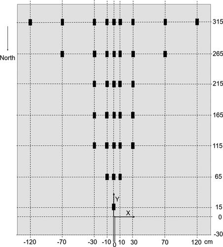
Table 1. Standard particle load per experiment.

Color	Size(μm)	Mass of Particle Load (mg)	Calculated number of Particles (#)
Green	180-212	25 ± 1	6.3$\times {10}^3$
Violet	45-53	25 ± 1	4.1$\times {10}^5$
Red	22-27	25 ± 1	3.7$\times {10}^6$

Deposition results are seen in Figures 10 and 11. The raw particle counts $r_{j,i}$ on strip j in test number i are normalized by the average centerline particle density, $\overline{C}$ (average density across all strips at location x = 0). This normalized data $n_{j,i}=r_{j,i}/\overline{C}$ more clearly indicates the relative particle deposition as a function of distance relative to the release point.

Figure 10. Centerline particle concentrations with standard deviation due to test–to–test variation indicated by error bars.

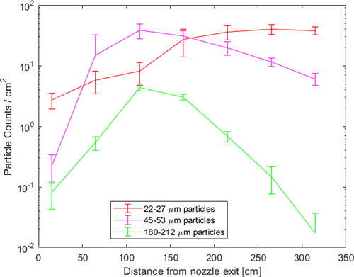
Figure 11. Average particle deposition results from ten repeat steady-state jet experiments for (a) 180–212 μm particles, (b) 22–27 μm particles, and (c) 45–53 μm particles.

The mean particle counts for each location are given in Table A3, as well as the standard deviation and relative error. The relative error is an indication of the range in which we expect the true mean to fall, and is computed using the sample standard deviation for each strip location, S_j, as follows: (5) $$\text{Relative}\mathrm{ }\text{Error}(\%)=100\left[t_{0.05,\nu }\frac{S_j}{m_{j,10}\sqrt{n}}\right]$$(5) where n = 10 is the number of samples and $t_{0.05,\nu }$ is read directly from a t-table for $\nu =n-1=9$ degrees of freedom. In this case a level of significance of 0.05 is used, corresponding to a 95% confidence interval. For strips with a mean of over 5 particles/strip the average relative uncertainty for 22–27 μm particles is 16.4%, 45–53 μm particles is 27.6%, and for 180–212 μm particles is 16.9%.

7. Illustrative comparison to CFD results

Calibration of numerical models is a motivating goal of our measurements. The previous section presents high–quality laboratory measurements of mid–size particle deposition in a quiescent, unobstructed, and carefully–characterized environment. To illustrate the potential of this data set for model calibration, we compare the data from these experiments to a common and widely implemented CFD modeling approach. The comparison is intentionally brief, serving solely to exemplify the utility of the data and highlight inherent challenges in predicting mid–size particle trajectories. We defer further development to future CFD–focused studies.

For the numerical computation of particle deposition patterns, we used the one–way–coupled Euler–Lagrange solver in ANSYS Fluent 2020 R2 to calculate the airflow field and particle trajectories. We developed a 955,000–cell unstructured poly–hexcore mesh to represent the geometry of the C³, leveraging the symmetry of C³ to reduce the size of the computational domain. A Reynolds Normalized Group (RNG) k–ϵ turbulence model with standard wall functions and Fluent–default model constants was used. Millions of individual particle trajectories were calculated in a Lagrangian framework using a discrete particle model (DPM) with high–resolution unsteady particle tracking and a discrete random walk (DRW) model to calculate the turbulent dispersion of particles. Default Fluent settings were used for the DPM length scale and DRW parameters.

Two different initial conditions were used to investigate model sensitivity and the basic jet dynamics. Case 1 begins with a quiescent background, so that the jets mean velocity structure is evolving at the same time that particles are being dispersed. Case 2 begins with the mean flow field produced by a turbulent jet which has been run until it reaches a statistically steady state; the particles are dispersed not by the mean jet but by a turbulent jet calculated from this initial condition. In both cases, the Eulerian field was run transiently with a max time–step of 0.1 s. The jet inlet was set to a constant and uniform velocity of 33.3 m/s for both air and particles throughout the release period (0 < t < 30 s) and both fields were allowed to transiently decay after t = 30 s.

As a comparison data set for the numerical results, contours of concentrations are computed through triangulation–based cubic interpolation of the experimental deposition data. The data is an average of the left– and right–hand side measurements in the deposition plane. During interpolation the experimental data is treated as a point–wise measurement at the center of the strip, but for clarity is shown in Figure 12 as a single concentration across the entire strip area.

Figure 12. Comparison of experimental results with CFD predictions of particle deposition from unsteady turbulent flow using initial flow fields that are quiescent (Case 1) and the mean flow from a steady-state jet (Case 2).

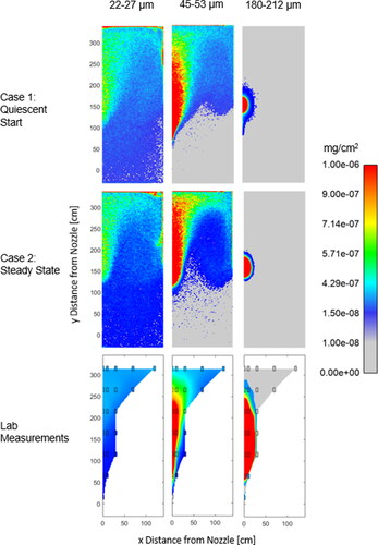
Figure 12 compares CFD predictions with the experimental data. The smallest particles (22–27 μm) spread further in the numerical result than in the laboratory result, and the largest particles (180–212 μm) spread less far in numerical result than in the laboratory result. Such differences require us to consider the good agreement for medium–size particles (45–53 μm) with some skepticism.

Numerical results can help us learn about the dynamics of the system, even if the particle transport is not yet in agreement with laboratory measurements. The transient starting effects, present in Case 1 but absent in Case 2, result in a predicted shift in the location of the peak amount of deposition toward the nozzle. This shift is seen by comparing the 45–53 and 180–212 μm particle profiles for the two cases. In Case 1, 45–53 and 180–212 μm particles are deposited in the region from approximately 50 cm < y < 125 cm near the centerline, which appears to be attributable to the use of a quiescent initial field. The lower velocity of the surrounding fluid imparts less momentum onto the suspended particles, leading to deposition closer to the nozzle as compared to Case 2. Conversely, in Case 2 we see an increase in the number of 45–53 μm, and to a lesser extent 22–27 μm, particles deposited in in the region y > 300 cm. The velocity field in Case 1 does not reach a steady state during the course of the injection (0 < t < 30 s), reaching a peak spatially averaged velocity of 0.095 m/s as compared to the fully developed value of 0.136 m/s across the domain; the fully developed velocity is the initial condition for Case 2 and remains constant during the release. The higher average velocity in Case 2 persists throughout the decay period, which appears to cause a higher portion of both the 22–27 and 45–53 μm particles to behave as aerosols; in turn, this increases the average particle residence time and the circulation of these particles throughout the chamber. The impact on the deposition pattern can be seen in Figure 12 with the increase in particles deposited in the area y < 100 cm far from the center-line.

8. Discussion

The COVID-19 pandemic motivated a number of practical transport studies in a variety of building and environmental airflow configurations. The boundary conditions in practical studies are by definition complex, and the large span of spatial scales (from the particles of interest to the room geometry) ensures that approximations are necessary for the problem to be tractable. The results of the present study highlight the importance of checking the validity of some common assumptions such as how well boundary conditions are defined. We were motivated by the concern that even the most careful treatment of boundary conditions (an already difficult task) may be insufficient for accurately predicting particle transport. We consider our results a promising message for the scientific community, because our data shows repeatability once we exert a level of environmental control that can be incorporated into many measurement setups.

The illustrative CFD comparison provided in Section 7 reinforces the complex issues involved with modeling the deposition of mid–range and ballistic–sized particles. Even when matching the quiescent background (despite the lack of flow obstructions, thermal gradients, particle evaporation, or electrostatic effects), there are clear areas in which more advanced CFD tools are needed to match the observed particle distribution. One is the turbulent transport of particles, in which particle clustering and/or anomalous diffusion (also called pre–Fickian or scale–dependent diffusion) can be important for certain points jet and particle conditions. Another is the interaction of the jet with walls and floors, which can be addressed through advanced CFD treatment of near–wall flows. CFD studies which attempt to model unstable and highly transient jet flows (such as a human cough) or capture effects such as evaporation must take additional care in ensuring that these effects are captured accurately.

The growing application and development of advanced CFD tools ensures that suitable experimental studies are needed for model validation, but as discussed in Section 1 such studies do not yet exist for practical geometries. Model validation experiments should carefully characterize or eliminate thermal gradients, ambient flows and charge effects. Methods for studying particle deposition must be accurate across a wide range of particle sizes, which is challenging with optical methods. The steps needed (e.g., room and sampling strip charge neutralization, and significant thermal insulation) suggests that in many studies that did not explicitly consider such effects and go to great lengths to mitigate them, results should be viewed cautiously with appreciation of the effects that may have affected the data yet not been described. We hope that future studies can build on the methods presented in this article to improve the quality of available validation studies. In the meantime, we hope that experimental studies in simplified geometries (such as the data presented in Section 6) see increased use in numerical model validation, as predicting mid–size particle transport is shown to be highly non–trivial.

9. Summary

Few experiments to date have studied the deposition of mid–range particles, i.e., those at the cross–over between aerosol and ballistic transport properties. To study these, it is essential to work in a quiescent, well–characterized environment, which takes significant work and thus is not always provided in otherwise excellent research. To address this gap in knowledge, methods for studying the deposition of droplets and particles were developed and applied to the creation of a dataset with well–characterized boundary conditions for numerical validation.

For studying the deposition of droplets, we explore and find promise in fluorescence–based sampling. Initial findings indicate that the deposition pattern of liquid droplets is strongly dependent on the ambient humidity; this relationship will be explored in greater depth in subsequent work.

Methods for studying the deposition of mid–range sized solid particles (22–212 μm) were presented in detail, followed by the study of deposition from a steady–state particle–laden turbulent jet with a mean velocity of 33.2 m/s and Re $\approx 21,500.$ The deposition location as a function of particle size was compared to results from a simple numerical RANS model, and found to need more work to bring the model dynamics and laboratory measurements into alignment. This result is not surprising given that the dispersal of particles by the turbulent jet does not follow a trivial scaling. Complexities include pre-Fickian (sometimes called “anomalous”) diffusion, spatial heterogeneity in the fundamental jet structure, and particles crossing fluid streamlines (Wang and Maxey 1993; Balachandar and Eaton 2010). In the course of the study, it also became clear that even modestly imprecise initial or boundary conditions in the model can lead to a notable deviation from laboratory results. This emphasizes that care needs to be taken on the experimental side to produce steady, uniform, and accurately measured boundary conditions.

In the gathering of this particle deposition dataset, we noted the extreme sensitivity in particle deposition patterns to the environment. In particular, we explore ways in which even small thermal gradients or electrostatic charge issues can affect the data. We provide practical methods to resolve these issues, including a new method of particle sampling using charge–neutralized adhesive sampling strips; this is coupled with cost–effective analysis utilizing a commercial flatbed scanner.

Despite working with a dataset from a quiescent, isothermal, and isopotential environment it was nontrivial to match the particle deposition pattern using RANS/DPM simulation of a particle–laden jet. As the COVID-19 pandemic motivates the need for study of droplet transport in increasingly complex environments we hope that this work provides an impetus to carefully examine those assumptions by which these works become tractable.

Acknowledgments

The authors gratefully acknowledge the gift of the Lam Research Corporation, and gifts coordinated through SEMI and provided by Advanced Energy Industries, Applied Materials, ASM, Entegris, JSR, KLA, TEL, and Wonik. Vision Research is thanked for providing a v2640 camera for a week to help quantify the particle velocities. Authors also gratefully acknowledge the valuable discussions with Brett Singer, Thomas Kirchstetter, Chelsea Preble of Lawrence Berkeley National Laboratory regarding droplet transport and COVID, and Keith Hansen on particle sampling and charge neutralization. We also thank Steven Ruzin, Director of the Biological Imaging Facility, for his assistance in obtaining the high–quality fluorescence microscopy images against which our particle counting method could be validated.

Additional information

Funding

We also acknowledge that this work began with the support of the 2020 Seed Fund Award 2020-0000000139 from the Center for Information Technology Research in the Interest of Society (CITRIS) and the Banatao Institute at the University of California. Research was supported by the DOE Office of Science through the National Virtual Biotechnology Laboratory, a consortium of DOE national laboratories focused on response to COVID-19, with funding provided by the Coronavirus CARES Act and the Department of Energy under Contract No. DEAC02-05CH11231.

Appendix A:

Temperature, relative humidity, and average particle deposition data

The wall temperatures are given in Table A1. The interior temperature relative humidity measurements for each test are given in Table A2. The absolute particle concentrations measured at each sampling strip are given in raw number of particle counts in Table A3. This is included to facilitate use of the data set for CFD code validation, which should be done using the local sampled values and not interpolated values of Figure 12. It is advisable to compare to deposition value normalized by the maximum or the center line average (as in Figure 11), as the true number of total particles deposited on the floor is largely unknown. While the number of particles injected to the launch apparatus is well-characterized (see Table 1), particles may be trapped in the ejection apparatus (either pipe or particle blaster), and may deposit in regions that are significantly under-sampled (such as far edges or walls of C³).

Table A1. Wall temperatures prior to test.

Experiment	N wall (${}^{°}$C)	W wall (${}^{°}$C)	S wall (${}^{°}$C)	E wall (${}^{°}$C)	Floor (${}^{°}$C)	Ceiling (${}^{°}$C)
1	23.8	24.0	23.8	23.6	23.0	23.3
2	24.4	24.6	24.6	24.6	24.3	24.6
3	24.8	24.8	24.7	24.8	24.8	24.9
4	24.4	24.6	24.4	24.5	24.4	24.5
5	24.7	24.5	24.5	24.5	24.3	24.4
6	24.3	24.7	24.4	24.4	24.4	24.6
7	24.1	24.2	24.2	24.2	24.1	24.5
8	24.3	24.1	24.4	24.1	23.9	24.2
9	24.0	24.0	24.2	24.0	23.7	24.1
10	23.9	24.4	24.1	24.1	23.6	23.8

Table A2. Interior temperature and relative humidity data during test.

Experiment	NW Temp. (${}^{°}$C)	NW RH (%)	SE Temp. (${}^{°}$C)	SE RH (%)
1	21.5	39.8	21.5	40.1
2	22.2	41.5	22.3	41.3
3	22.8	36.4	22.8	37.2
4	22.4	52.5	22.4	53.5
5	22.5	51.4	22.4	52.8
6	22.3	36.8	22.3	38.0
7	22.3	41.7	22.2	43.1
8	22.1	35.0	22.1	35.8
9	22.1	41.4	22.1	42.5
10	21.9	40.4	21.9	41.4

Table A3. Raw deposition data listing average number of particles per 51.6 cm² strip centered at the given x and y location.

		22–27 μm			45–53 μm			180–212 μm
x [cm]	y [cm]	average counts	std. dev	Relative Error %	average counts	std. dev	Relative Error %	average counts	std. dev	Relative Error %
−120	315	2230	446	11.6	237	48	11.7	0.1	0.3	183.3
−70	265	1484	433	16.9	193	132	39.7	0	0.0
−70	315	2036	449	12.8	257	61	13.7	0	0.0
−30	115	392	125	18.4	16	8	31.2	0.3	0.7	130.4
−30	165	573	139	14.1	30	10	20.5	1.2	1.1	54.8
−30	215	1087	405	21.6	338	226	38.8	2.1	2.0	55.9
−30	265	2037	389	11.1	487	187	22.3	2	1.7	49.3
−30	315	2043	463	13.1	326	107	19.0	0.8	1.0	74.8
−10	65	243	71	16.9	15	6	22.0	3.4	2.1	35.2
−10	115	344	111	18.7	295	396	77.8	96.8	26.0	15.6
−10	165	807	233	16.7	918	314	19.8	83.2	14.9	10.4
−10	215	1745	602	20.0	909	393	25.0	21.7	5.1	13.6
−10	265	1998	360	10.5	556	136	14.2	5	3.3	38.3
−10	315	1949	451	13.4	308	87	16.4	1	1.2	72.3
0	15	141	42	17.1	12	6	28.2	4.2	2.0	27.5
0	65	299	122	23.8	767	904	68.4	27.9	7.0	14.6
0	115	417	169	23.5	1961	541	16.0	227.3	29.8	7.6
0	165	1393	674	28.0	1583	344	12.6	157.3	16.4	6.0
0	215	1875	511	15.8	1023	255	14.4	35.5	6.8	11.1
0	265	2083	364	10.1	596	95	9.3	7.5	3.6	27.6
0	315	1955	286	8.5	313	69	12.8	0.9	1.0	64.1
10	65	276	96	20.1	55	104	110.1	8.9	3.7	24.3
10	115	332	106	18.6	553	445	46.6	129.6	16.8	7.5
10	165	1060	657	35.9	988	200	11.7	87	22.4	14.9
10	215	2046	655	18.6	929	330	20.6	24.8	9.6	22.3
10	265	1973	370	10.9	513	91	10.3	5.4	2.1	22.7
10	315	1851	255	8.0	296	63	12.3	1.2	1.0	49.9
30	115	415	133	18.6	19	9	28.0	0.2	0.6	183.3
30	165	603	187	17.9	129	128	57.6	1.5	1.6	63.8
30	215	1523	846	32.2	522	364	40.4	2.9	2.1	41.6
30	265	1840	409	12.9	405	108	15.4	1.5	1.2	45.5
30	315	1732	144	4.8	254	64	14.7	0.5	0.7	82.0
70	265	1364	291	12.4	137	73	30.7	0	0.0
70	315	1711	341	11.6	223	64	16.5	0	0.0
120	315	1909	352	10.7	215	65	17.6	0	0.0

References

- Bahl, P., C. Doolan, C. De Silva, A. A. Chughtai, L. Bourouiba, and C. R. MacIntyre. 2020. Airborne or droplet precautions for health workers treating COVID-19? Clin. Infect. Dis. 24 (17):1639–41. doi:10.1093/infdis/jiaa189
- Balachandar, S., and J. K. Eaton. 2010. Turbulent dispersed multiphase flow. Ann. Rev. Fluid Mech. 42 (1):111–33. doi:10.1146/annurev.fluid.010908.165243.
- Bolster, D. T., and P. F. Linden. 2009. Particle transport in low-energy ventilation systems. Part 2: Transients and experiments. Indoor Air. 19 (2):130–44. doi:10.1111/j.1600-0668.2008.00569.x.
- Bordoloi, A. D., C. C. K. Lai, L. Clark, G. V. Carrillo, and E. Variano. 2020. Turbulence statistics in a negatively buoyant multiphase plume. J. Fluid Mech. 896:A19. doi:10.1017/jfm.2020.326.
- Bourouiba, L. 2016. A Sneeze. N. Engl. J. Med. 375 (8):e15. doi:10.1056/NEJMicm1501197.
- Bourouiba, L., E. Dehandschoewercker, and J. W. Bush. 2014. Violent expiratory events: On coughing and sneezing. J. Fluid Mech. 745:537–63. doi:10.1017/jfm.2014.88.
- Chao, C. Y., and M. P. Wan. 2006. A study of the dispersion of expiratory aerosols in unidirectional downward and ceiling-return type airows using a multiphase approach. Indoor Air 16 (4):296–312. doi:10.1111/j.1600-0668.2006.00426.x.
- Chu, D. K., E. A. Akl, S. Duda, K. Solo, S. Yaacoub, H. J. Schünemann, D. K. Chu, E. A. Akl, A. El-Harakeh, A. Bognanni, et al. 2020. Physical distancing, face masks, and eye protection to prevent person-to-person transmission of SARS-CoV-2 and COVID-19: A systematic review and meta-analysis. Lancet 395 (10242):1973–87. doi:10.1016/S0140-6736(20)31142-9.
- Einstein, H. A., and H. W. Shen. 1964. A study on meandering in straight alluvial channels. J. Geophys. Res. 69 (24):5239–47. doi:10.1029/JZ069i024p05239.
- Elghobashi, S. 1994. On predicting particle-laden turbulent flows. Appl. Sci. Res. 52 (4):309–29. doi:10.1007/BF00936835.
- Elgobashi, S. 2006. An updated classification map of particle-laden turbulent flows. In IUTAM Symposium on Computational Approaches to Multiphase Flow, 3–10. Springer.
- Guazzelli, E., and J. F. Morris. 2011. A physical introduction to suspension dynamics. Vol. 45. New York: Cambridge University Press.
- Hinds, W. C. 1999. Aerosol technology: Properties, behavior, and measurement of airborne particles. New York: John Wiley & Sons.
- Jayaweera, M., H. Perera, B. Gunawardana, and J. Manatunge. 2020. Transmission of COVID-19 virus by droplets and aerosols: A critical review on the unresolved dichotomy. Environ. Res. 188:109819. doi:10.1016/j.envres.2020.109819.
- Jin, H., Q. Li, L. Chen, J. Fan, and L. Lu. 2009. Experimental analysis of particle concentration heterogeneity in a ventilated scale chamber. Atmos. Environ. 43 (28):4311–8. doi:10.1016/j.atmosenv.2009.06.002.
- Jones, R. M., and M. Nicas. 2014. Experimental evaluation of a Markov multizone model of particulate contaminant transport. Ann. Occup. Hyg. 58 (8):1032–45.
- Jones, R., and M. Nicas. 2009. Experimental determination of supermicrometer particle fate subsequent to a point release within a room under natural and forced mixing. Aerosol Sci. Technol. 43 (9):921–38. doi:10.1080/02786820903036322.
- Jurelionis, A., L. Gagytė, T. Prasauskas, D. Čiužas, E. Krugly, L. Šeduikytė, and D. Martuzevičius. 2015. The impact of the air distribution method in ventilated rooms on the aerosol particle dispersion and removal: The experimental approach. Energy Build. 86:305–13. doi:10.1016/j.enbuild.2014.10.014.
- Kohanski, M. A., L. J. Lo, and M. S. Waring. 2020. Review of indoor aerosol generation, transport, and control in the context of COVID-19. Int. Forum Allergy Rhinol. 10 (10):1173–9. In 10. Wiley Online Library. doi:10.1002/alr.22661.
- Lai, A. C., and S.-L. Wong. 2010. Experimental investigation of exhaled aerosol transport under two ventilation systems. Aerosol Sci. Technol. 44 (6):444–52. doi:10.1080/02786821003733826.
- Lee, J., D. Yoo, S. Ryu, S. Ham, K. Lee, M. Yeo, K. Min, and C. Yoon. 2019. Quantity, size distribution, and characteristics of cough-generated aerosol produced by patients with an upper respiratory tract infection. Aerosol Air Qual. Res. 19 (4):840–53. doi:10.4209/aaqr.2018.01.0031.
- Lindsley, W. G., W. P. King, R. E. Thewlis, J. S. Reynolds, K. Panday, G. Cao, and J. V. Szalajda. 2012. Dispersion and exposure to a cough-generated aerosol in a simulated medical examination room. J. Occup. Environ. Hyg. 9 (12):681–90. doi:10.1080/15459624.2012.725986.
- Liu, S., and A. Novoselac. 2014. Transport of airborne particles from an unobstructed cough jet. Aerosol Sci. Technol. 48 (11):1183–94. doi:10.1080/02786826.2014.968655.
- Liu, Z. W., Zhuang, L. Hu, R. Rong, J. Li, W. Ding, and N. Li. 2020. Experimental and numerical study of potential infection risks from exposure to bioaerosols in one BSL-3 laboratory. Build. Environ. 179:106991. doi:10.1016/j.buildenv.2020.106991.
- Matsuyama, T. 2018. A discussion on maximum charge held by a single particle due to gas discharge limitation. In AIP Conference Proceedings. Vol. 1927, 020001. AIP Publishing LLC.
- Miller, S. L., and W. W. Nazaroff. 2001. Environmental tobacco smoke particles in multizone indoor environments. Atmos. Environ. 35 (12):2053–67. doi:10.1016/S1352-2310(00)00506-9.
- Murakami, S. 1992. Diffusion characteristics of airborne particles with gravitational setting in an convection-dominant indoor flow field. Ashrae Trans. 98 (1):82–97.
- Nissen, K., J. Krambrich, D. Akaberi, T. Hoffman, J. Ling, Å. Lundkvist, L. Svensson, and E. Salaneck. 2020. Long-distance airborne dispersal of SARS-CoV-2 in COVID-19 wards. Sci. Rep. 10 (1):19589. doi:10.1038/s41598-020-76442-2.
- Picano, F., G. Sardina, and C. M. Casciola. 2009. Spatial development of particle-laden turbulent pipe flow. Phys. Fluids 21 (9):093305. doi:10.1063/1.3241992.
- Qian, H., and Y. Li. 2010. Removal of exhaled particles by ventilation and deposition in a multibed airborne infection isolation room. Indoor Air. 20 (4):284–297. doi:10.1111/j.1600-0668.2010.00653.x.
- Richmond-Bryant, J., A. D. Eisner, L. A. Brixey, and R. W. Wiener. 2006. Transport of airborne particles within a room. Indoor Air. 16 (1):48–55. doi:10.1111/j.1600-0668.2005.00398.x.
- Sajo, E., H. Zhu, and J. C. Courtney. 2002. Spatial distribution of indoor aerosol deposition under accidental release conditions. Health Phys. 83 (6):871–883.
- Seepana, S., and A. C. Lai. 2012. Experimental and numerical investigation of interpersonal exposure of sneezing in a full-scale chamber. Aerosol Sci. Technol. 46 (5):485–493. doi:10.1080/02786826.2011.640365.
- Stan, C. A., D. Milathianaki, H. Laksmono, R. G. Sierra, T. A. McQueen, M. Messerschmidt, G. J. Williams, J. E. Koglin, T. J. Lane, M. J. Hayes, et al. 2016. Liquid explosions induced by X-ray laser pulses. Nature Phys. 12 (10):966–972. doi:10.1038/nphys3779.
- Sze To, G. N., M. P. Wan, C. Y. Chao, F. Wei, S. C. Yu, and J. K. Kwan. 2008. A methodology for estimating airborne virus exposures in indoor environments using the spatial distribution of expiratory aerosols and virus viability characteristics. Indoor Air. 18 (5):425–438. doi:10.1111/j.1600-0668.2008.00544.x.
- Taghavivand, M., P. Mehrani, A. Sowinski, and K. Choi. 2021. Electrostatic charging behaviour of polypropylene particles during pulse pneumatic conveying with spiral gas flow pattern. Chem. Eng. Sci. 229:116081. doi:10.1016/j.ces.2020.116081.
- Tang, J. W., W. P. Bahnfleth, P. M. Bluyssen, G. Buonanno, J. L. Jimenez, J. Kurnitski, Y. Li, S. Miller, C. Sekhar, L. Morawska, et al. 2021. Dismantling myths on the airborne transmission of severe acute respiratory syndrome coronavirus-2 (SARS-CoV-2)). J. Hosp. Infect. 110:89–96. doi:10.1016/j.jhin.2020.12.022
- Wan, M. P., C. Yu, H. Chao, Y. D. Ng, G. Nam Sze To, and W. C. Yu. 2007. Dispersion of expiratory droplets in a general hospital ward with ceiling mixing type mechanical ventilation system. Aerosol. Sci. Technol. 41 (3):244–258. doi:10.1080/02786820601146985.
- Wang, L.-P., and M. R. Maxey. 1993. Settling velocity and concentration distribution of heavy particles in homogeneous isotropic turbulence. J. Fluid Mech. 256:27–68. doi:10.1017/S0022112093002708.
- Wang, B., H. Wu, and X.-F. Wan. 2020. Transport and fate of human expiratory droplets-A modeling approach. Phys. Fluids (1994) 32 (8):083307. doi:10.1063/5.0021280.
- Wei, J., and Y. Li. 2015. Enhanced spread of expiratory droplets by turbulence in a cough jet. Build. Environ. 93:86–96. doi:10.1016/j.buildenv.2015.06.018.
- Wei, J., and Y. Li. 2017. Human cough as a two-stage jet and its role in particle transport. PloS One. 12 (1):e0169235. doi:10.1371/journal.pone.0169235.
- Yang, S., G. W. Lee, C.-M. Chen, C.-C. Wu, and K.-P. Yu. 2007. The size and concentration of droplets generated by coughing in human subjects. J. Aerosol. Med. 20 (4):484–494. doi:10.1089/jam.2007.0610.
- Yang, W., and L. C. Marr. 2011. Dynamics of airborne inuenza A viruses indoors and dependence on humidity. PloS One. 6 (6):e21481. doi:10.1371/journal.pone.0021481.
- Zhang, Z., and Q. Chen. 2006. Experimental measurements and numerical simulations of particle transport and distribution in ventilated rooms. Atmos. Environ. 40 (18):3396–3408. doi:10.1016/j.atmosenv.2006.01.014.
- Zhang, Z., X. Chen, S. Mazumdar, T. Zhang, and Q. Chen. 2009. Experimental and numerical investigation of airflow and contaminant transport in an airliner cabin mockup. Build. Environ. 44 (1):85–94. doi:10.1016/j.buildenv.2008.01.012.
- Zhang, N., Z. Zheng, S. Eckels, V. B. Nadella, and X. Sun. 2009. Transient response of particle distribution in a chamber to transient particle injection. Part. Part. Syst. Charact. 26 (4):199–209. doi:10.1002/cncr.29118.
- Zhu, S., S. Kato, and J.-H. Yang. 2006. Study on transport characteristics of saliva droplets produced by coughing in a calm indoor environment. Build. Environ. 41 (12):1691–1702. doi:10.1016/j.buildenv.2005.06.024.
- Zohdi, T. I. 2020. Modeling and simulation of the infection zone from a cough. Comput. Mech. 66 (4):1–1034. doi:10.1007/s00466-020-01875-5.