The performance of an electrical ionizer as a bipolar aerosol charger for charging ultrafine particles

Abstract

We developed an aerosol charger that incorporated commercial ionizers to make the setup simple and easily replicated. The built-in high-voltage source for inducing corona discharge embedded in the developed charger (MHM charger) was modulated with pulses so the production of positive and negative ions could be independently regulated. We have studied several attempts to evaluate the performance of the MHM charger as a bipolar charger for charging ultrafine particles. We found that by adjusting the duty-cycle of the modulated pulses, positive and negative ion production is manageable, and the ion concentration depends on the flow rate of the intake air. We used a mini-cyDMA to measure the mobility distribution of positive and negative ions with an average of 1.09 and 1.67 cm² V⁻¹ s⁻¹, respectively. By utilizing initially charged and neutral particles, we obtained the penetration ratio of both particles: 0.75 and 0.774, respectively. The issue of the MHM charger to generate new particles was also investigated. We found that, on average, the produced new particle concentration was only 5.2 cm⁻³. In this study, we evaluated the performance of the MHM charger to charge particles by measuring the neutral fraction and charging efficiency. The neutral fraction with particle loss correction follows the established model. The intrinsic and extrinsic charging efficiencies at 100 nm were up to 19% and 41%, respectively. We also assessed the application of the MHM charger in the monodisperse particle generator system. The results showed that the MHM charger could be utilized as an alternative aerosol charger.

Copyright © 2021 American Association for Aerosol Research

EDITOR:

• Jason Olfert

1. Introduction

One of the most significant subjects in the aerosol measurement system is the electrical charging of particles by ions (Alonso et al. 1997b). It is understandable since the aerosol charger device is a critical part of the electric-based aerosol measurement system. For instance, when we use a differential mobility analyzer (DMA), particles must be charged before flowing into the DMA system. When the measured aerosol particles are neutral, the charger is used for charging the particles. Meanwhile, when the measured aerosol particles are initially charged, for example, due to direct contact charging (Forsyth, Liu, and Romay 1998), it requires the charger to reduce the multicharged particles. By considering the vital role of the aerosol charger in measurement, it is necessary to investigate the performance of the aerosol charger.

There are several types of aerosol chargers that have been developed based on radio-ionization (Clement and Harrison 1992; Liu, Pui, and Lin 1986; Okuyama, Kitada, and Motouchi 1983), photoionization (Nishida, Boies, and Hochgreb 2018; Hontañón and Kruis 2008; Shimada et al. 2002), or electric field ionization (Qi and Kulkarni 2013; Kwon et al. 2005; Stommel and Riebel 2004; Whitby 1961). A charger employing a radioactive source utilizes radioactive decay to produce ions in the air. Generally, radioactive-based chargers equally generate positive and negative ions (Clement and Harrison 1992). Radioactive source use is usually costly and involves strict regulation (Kimoto et al. 2009; IAEA 2005). In Indonesia, it is restricted by the National Nuclear Energy Agency of Indonesia.¹ Such restriction is also found in other countries, such as Japan (Kimoto et al. 2009). Another type of charger uses X-rays to produce high concentration ions (Shimada et al. 2002), yet it also has the same legal restrictions as the radioactive sources. Since it is difficult to get those chargers, we can use the corona discharge-based charger as an alternative charger. Despite several issues, such as the unbalanced production of ions, generated ozone, and particles produced by sputtering or chemical reactions (Romay, Liu, and Pui 1994), there are ways of improving the corona-based charger performance. For instance, we could develop an electrode with a particular geometry to reduce ozone generation (Kwon et al. 2005), optimize the electrode's length (Osone et al. 2012), or optimize the waveform of high-voltage sources to improve charging efficiency (Manirakiza et al. 2013).

Bipolar ions can be produced using dual corona ionizers, as Adachi, Kousaka, and Okuyama (1985) and Romay, Liu, and Pui (1994) developed. However, according to Qi and Kulkarni (2013), the development of the dual corona ionizer had a complexity that made it hard to use in field-portable, compact instrumentation. Hence, Qi and Kulkarni (2013) made a compact, miniature, and low-cost dual corona bipolar charger (DCBC) applied in portable, hand-held mobility-size spectrometers. However, the development of the instrumentation was rather complex, where the corona is induced by using a constant current so that a closed-loop control system is needed. Moreover, the proportional-integral-derivative controller must be tuned to find the optimum control constant, which may have different values for each set of DCBC systems.

Therefore, we aimed to develop a low-cost bipolar aerosol charger using a dual corona ionizer with a simple circuit arrangement, which can independently adjust positive and negative ion concentration and is suitable for field-portable use. In specific applications, the low-cost corona-based charger would be more beneficial compared with a radioactive-based charger. For instance, to reach the stationary charging state, the use of radioactive sources would require high activity, which is more expensive. Ibarra, Rodríguez-Maroto, and Alonso (2020) found that the stationary charge distribution cannot be achieved on the commercial radioactive-based charger of either low activity or 2 mCi. Moreover, the low-cost corona-based charger could also be applied along with an ion trap and Faraday cup electrometer for low-cost monitoring of airborne particle concentration, as Nishida et al. (2020) developed, or as a charger component in a particle sizer system with an inexpensive and lightweight differential mobility analyzer (Barmpounis et al. 2016).

The developed aerosol charger consists of low-cost commercial electrical ionizers, a high-voltage (HV) driver system, and a cylindrical chamber. A commercial ionizer is expected to provide consistent characteristics, which will be easily replicated without detailed characterization. However, commercial ionizers generally have a fixed built-in HV source. Therefore, to regulate and control ion production, we applied a pulse modulation. The characterizations of the aerosol charger were determined by investigating the ion distribution, ion production on a varied duty-cycle configuration and flow rate, new particle generation, particle penetration, and charging probability. The implementation of the aerosol charger to determine the particle mobility distribution is also discussed.

2. Experimental

2.1. Description of SMAC and MHM charger

A surface-discharge micro-plasma aerosol charger (SMAC) had been developed and investigated by Kwon et al. (2005, 2006). SMAC is a dielectric barrier discharge (DBD) with a surface-discharged (SD) arrangement. Generally, there are two types of DBD arrangements, surface discharged (SD) and volume discharged (VD) (Gibalov and Pietsch 2000). SMAC is composed of a specially designed electrode (serrated electrode) and uses DC pulse to induce the surface discharge. The use of DC pulse to induce corona discharge was also previously studied (Liu and Neiger 2001). The SMAC configuration that we used is shown in Figures 1a and c. Figure 1a shows a stainless-steel chamber equipped with SMACs in the upper lid and bottom lid. One SMAC was supplied with a negative high-voltage (HV) DC pulse. The other one was supplied with a positive HV DC pulse to produce negative and positive ions, respectively, and as a result, we could obtain stable bipolar ions.

Figure 1. (a, b) The structures of SMAC and the MHM charger. (c, d) The schematic diagrams of SMAC and the MHM charger.

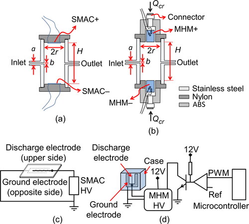
We developed a bipolar aerosol charger (the MHM charger) by incorporating commercially available devices. In this work, electrical ionizer modules fabricated by Murata Manufacturing Co., Ltd., Japan, were used as ion sources. We used the MHM 305-01 model (referred to as MHM–) and the MHM 400-01 model (referred to as MHM+) to produce negative and positive ions, respectively. Considering the MHM datasheet, we chose these two MHM modules because they could effectively generate ions with low ozone levels, less than 0.5 ppm. The MHM + and MHM– were placed opposite each other on the chamber lids, as shown in Figure 1b. The chamber is made of stainless steel, the same as the SMAC chamber; the only difference between these two chambers is their lids. Both the SMAC and MHM charger have an effective chamber volume of 115.6 cm³ (r = 2 cm, H = 9.2 cm, a = 6 mm, and b = 4 mm), and the corresponding residence time is 6.9 s when the aerosol flow rate is 1 L min⁻¹. Figure S4 depicts a photograph of the MHM charger. The MHM module case, as shown in Figure 1d, has a hollow that allows the lid (Figure 1b) to have a clean air inlet line, Q_cr. However, we did not use the clean air inlet in this work (Q_cr = 0). The effect of Q_cr on the performance of the MHM charger will be thoroughly discussed later in other sections.

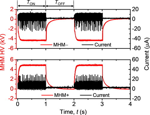
Figure 1d shows the MHM module electrode with a VD arrangement with an air gap. A discharge electrode was placed amid the ground electrode, which adheres to a dielectric substrate. The HV has a peak-to-peak ripple voltage of 276 V and 237 V for MHM + and MHM–, respectively. When the HV is higher than the breakdown voltage, the edge of the discharge electrode generates several micro discharges. The energy released by the micro discharges would dissociate surrounding molecules and therefore produce ions. HV used by MHM modules (referred to as MHM HV) has an input working DC voltage of 12 V. We developed a driver system using a transistor (Model TIP122, Semiconductor Components Industries, LLC., USA), as shown in Figure 1d. To amplify pulse width modulation (PWM) voltage from a microcontroller (Model ATMega328p, Atmel Corp., USA), we utilized an operational amplifier (Model LM393, Semiconductor Components Industries, LLC., USA). Hence, the MHM HV will periodically be in the ON and OFF conditions. The duration of the ON condition (T_ON) and OFF condition (T_OFF) is represented by the duty-cycle (D). By utilizing the embedded system, we could easily change the D parameter through a user interface, (1) $$D_{\pm }=\frac{T_{\mathrm{ON}\pm }}{T_s}\times 100\%,$$(1) where T_s = T_ON + T_OFF. Positive (+) and negative (–) subscripts represent the parameter for both MHM + and MHM–, respectively. According to the datasheet, the T_OFF of MHM HV must be higher than 1 s. For that reason, we set the PWM period (T_s) at 2 s so that the maximum duty-cycle used is up to 50%. Figure 2 depicts the MHM HV output voltage and corona current generated by both MHM + and MHM– modules after being modulated with a duty-cycle of 50%. The output voltage and current were measured using an OWON oscilloscope (Model SDS1102, OWON Technology Inc., Canada). The current was measured by adding a 330 Ω load.

Figure 2. The pulse width modulated voltage signal of MHM + and MHM–.

2.2. Ion mobility and concentration

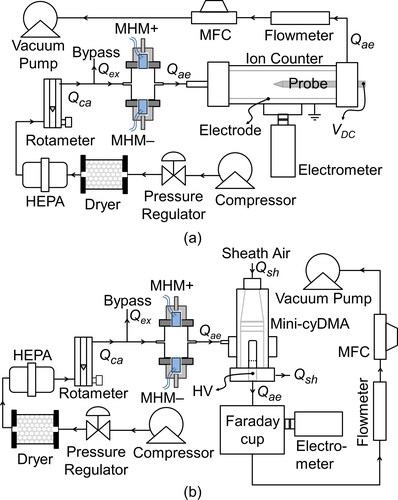
The measurement of ion concentration produced by the MHM charger could be performed by utilizing an ion counter system with the same experimental setup done by Yun, Otani, and Emi (1997) (see Figure 3a). A dry and clean air supply (Q_ca) was obtained by flowing compressed air through a dryer and HEPA filter. Q_ca was controlled by a rotameter and regulated at 3 L min⁻¹. The airflow drawn by the ion counter using a vacuum pump, Q_ae, was controlled by a self-designed mass flow controller (MFC) and monitored by a flowmeter (Model AWM5101VN, Honeywell International, Inc., USA). The residual air, Q_ex = Q_ca – Q_ae, was taken out through a bypass that works to avoid contamination from the surrounding air and to assure that the experiment ran at atmospheric pressure. The probe was supplied with +12 V when we wanted to measure positive ions. Meanwhile, to measured negative ions, the probe was supplied with −12 V. The voltage on the probe produced an electric field so that the measured ions would move toward the electrode, while the residual ions would be pulled toward the probe. The number of ions stuck on the electrode was measured by a supersensitive electrometer with a measurement range of −1 × 10⁴ to 1 × 10⁴ fA and a resolution up to 1 fA. The ion concentration is determined using the following formula (Munir et al. 2013; Yun, Otani, and Emi 1997): (2) $$n_{\pm }=\frac{|I-I_o|}{e{Q}_{ae}},$$(2) where n is either a positive (+) ion or negative (–) ion concentration. I, I_o, and e represent the current measured by the electrometer, reading offset of the electrometer, and electron charge, respectively.

Figure 3. The experimental setups for measuring (a) ion concentration and (b) ion mobility.

The effect of duty-cycle and airflow rate on ion concentrations was also characterized. As for the effect of the duty-cycle, we varied the D_± configuration. To simplify the labeling, we wrote the configuration of D₊ and D_– as P(D₊)N(D_–). For instance, P20N30 means that the MHM + and MHM– were set simultaneously at duty-cycles of D₊ = 20% and D_– = 30%, respectively. We varied the duty-cycle of both MHM + and MHM– with the range of 10% to 50% at Q_ae = 1 L min⁻¹. The airflow rate effect was characterized by varying Q_ae from 0.25 to 1.5 L min⁻¹ at P50N50.

The ion mobility was measured using a miniature cylindrical differential mobility analyzer (mini-cyDMA), designed to measure ion clusters sized less than 3 nm in diameter. The developed mini-cyDMA is the same as the mini-cyDMA Cai et al. (2017) made, which consists of a column of 16.2 mm in length, with an inner and outer radius of 3.5 mm and 10 mm, respectively. The experimental setup to measure ion mobility is shown in Figure 3b. The sheath airflow rate (Q_sh) and aerosol flow rate (Q_ae) were set at 20 L min⁻¹ and 1 L min⁻¹, respectively. The dry and clean air (Q_ca) and drawn aerosol flow system (Q_ae) were supplied the same way as the ion concentration measurement setup. The HV voltage was gradually adjusted with a range of 5 − 64 V at negative- and positive-DC polarization. The separated ions (based on their mobility) were then transferred to a Faraday cup (Intra and Tippayawong 2009) to measure the generated current using an electrometer simultaneously.

2.3. Evaluation of the MHM charger performance

All the evaluations of the MHM charger in this article employed NaCl particles generated from 5 wt% NaCl solution, atomized using jet atomizer (Nebulizer Kit, Model NE-C28, Omron Healthcare Co., Ltd., Japan). The NaCl solution contains 5 parts of the NaCl powder mass (58.44 g mol⁻¹, Millipore Corp., Germany) in 95 parts of the mass of water solvent (Water for Injection, PT. Ikapharmindo Putramas, Indonesia). The monodispersed charged NaCl particles were generated using a monodisperse particle generator (MPG). Figures 4b–d depict the experimental setup, the same as the setup used by Kwon et al. (2006) and Manirakiza et al. (2013). The MPG setup is shown in Figure 4e, where the MPG outlet is downstream of a long differential mobility analyzer (LDMA) with a sheath airflow of 10 L min⁻¹, as Song et al. (2006) used. Compressed dry and clean air flowed into a jet atomizer (Q_neb), and clean dilute air (Q_dil) were set at 1.5 and 5 L min⁻¹, respectively.

Figure 4. The experimental setups for evaluating (a) new particle formation by the chargers, (b) the charged particle penetration ratio of the chargers, (c) the neutral particle penetration of the MHM charger, (d) the charging probability, and (e) the electrical mobility distribution.

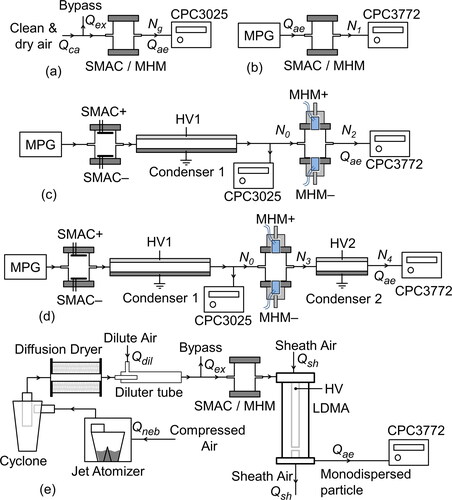
In this work, two condensation particle counters (CPCs) (Model 3025 and 2772, TSI Inc., USA) were used for measuring particle concentration. Before being used, we benchmarked the reading of CPC3025 and CPC3772. The reading value of CPC3025 used in all calculations was corrected with the N_rel factor (see supplementary information [SI], section 1).

Before evaluating the MHM charger, we measured the new generated particle concentration using CPC3025, since the plasma chargers usually have trouble with particle generation due to sputtering, including the surface discharge. The experimental scheme for measuring the number of new generated particles is shown in Figure 4a. In addition, the experimental setups in Figures 4b–d were used to measure particle penetration with a charged-particle source; particle penetration with a neutral-particle source; and total penetration of the MHM charger and Condenser 2, neutral fraction and charging efficiency, respectively. To clarify the evaluation of the associated parameters, we list them in Table 1.

Table 1. Summary of the measured parameters, experimental condition, and calculation used for evaluating the MHM charger.

Setup	The measured parameters	Experimental conditions	Calculation	Equation
Figure 4a	New particle generation	SMAC/MHM charger: ON	Ng
Figure 4b	Charged-particle penetration ratio (rc)	SMAC/MHM charger: ON and OFF	$r_c=\frac{N_1^{\mathrm{ON}}}{N_1^{\mathrm{OFF}}}$	(3)
Figure 4c	Neutral-particle penetration when the MHM charger was in the OFF condition (ηn^OFF)	SMAC: ON Condenser 1: ON MHM charger: OFF	${\eta }_n^{\mathrm{OFF}}=\frac{N_2^{\mathrm{OFF}}}{N_0^n}$	(4)
Figure 4c	Neutral-particle penetration when the MHM charger was in the ON condition (ηn^ON)	SMAC: ON Condenser 1: ON MHM charger: ON	${\eta }_n^{\mathrm{ON}}=\frac{N_2^{\mathrm{ON}}}{N_0^n}$	(5)
Figure 4d	The total neutral-particle penetration of the MHM charger and Condenser 2 when both of them were in the OFF condition (ξn^OFF)	SMAC: ON Condenser 1: ON MHM charger: OFF Condenser 2: OFF	${\xi }_n^{\mathit{OFF}}=\frac{N_4^{\mathrm{OFF}}}{N_0^n}$	(6)
Figure 4d	The total charged-particle penetration of the MHM charger and Condenser 2 when both of them were in the OFF condition (ξc^OFF)	SMAC: OFF Condenser 1: OFF MHM charger: OFF Condenser 2: OFF	${\xi }_c^{\mathit{OFF}}=\frac{N_4^{\mathrm{OFF}}}{N_0^c}$	(7)
Figure 4d	Neutral fraction (f0)	SMAC: ON Condenser 1: ON MHM charger: ON Condenser 2: ON and OFF	$f_0=\frac{N_4^{\mathrm{ON}}}{N_4^{\mathrm{OFF}}}$	(8)
Figure 4d	Intrinsic charging efficiency (ηintr)	SMAC: ON Condenser 1: ON MHM charger: ON Condenser 2: ON	${\eta }_{\mathit{intr}}=\frac{{\eta }_n^{\mathrm{OFF}}{N}_0^n-N_4^{\mathrm{ON}}}{N_0^n}$	(9)
Figure 4d	Extrinsic charging efficiency (ηextr)	SMAC: ON Condenser 1: ON MHM charger: ON Condenser 2: ON and OFF	${\eta }_{\mathit{extr}}=\frac{N_4^{\mathrm{OFF}}-N_4^{\mathrm{ON}}}{N_0^n}$	(10)

The index n and c indicate neutral and charged particles used as the source, respectively. The index ON and OFF indicate that either the charger or condenser was in the ON and OFF condition, respectively. N_g and N_0–4 are particle concentrations specifically at a particular location, as shown in Figure 4. The neutral-particle penetration ratio is the ratio of neutral-particle penetration when the MHM charger was in the ON and OFF condition, r_n = η_n^ON/η_n^OFF. We measure the penetration of the total particles of the MHM charger and Condenser 2 because it will be needed later to calculate the neutral fraction correction.

We set both SMAC and Condenser 1 to OFF and ON, respectively, to obtain neutral and charged particles source, as shown in Figures 4c and d. The MPG outlet, monodispersed charged particle, was delivered to and then neutralized by the SMAC. The remaining charged particles were removed by passing them through Condenser 1, which utilizes HV1 of −5 kV. In this condition, the collection efficiency of Condenser 1 was ∼100% for particles under 250 nm. Meanwhile, Condenser 2 was set to ON to trap charged particles after the particles were recharged by the MHM charger. The collection efficiency of Condenser 2 was ∼100% for particles under 100 nm. Details about the collection efficiency of both Condenser 1 and 2 can be seen in the SI, section 2.

The charging probability (P_c) of the initially neutral particle can be obtained by determining the charged-particle fraction, P_c = 1 – f₀. The presence of particle loss in the MHM charger and Condenser 2 can make an inaccurate calculation from Equation (8). Consequently, we need to apply particle loss correction so the following equation can calculate the neutral fraction without particle loss (f₀'), (11) $$f_0^{\prime }=\frac{N_4^{\mathrm{ON}}}{\frac{{\xi }_n^{\mathrm{OFF}}}{{\xi }_c^{\mathrm{OFF}}{r}_c}{N}_4^{\mathrm{OFF}}+\left(1-\frac{{\xi }_n^{\mathrm{OFF}}}{{\xi }_c^{\mathrm{OFF}}}\right)N_4^{\mathrm{ON}}}.$$(11)

Nonetheless, both the intrinsic and extrinsic charging efficiency expressed by Equations (9)(A2) $$L=\frac{N_0^n-N_2^{ON}}{N_0^n}=1-{\eta }_n^{ON}.$$(A2) and (10(A3) $$L_e=\frac{N_2^{\mathit{OFF}}-N_2^{ON}}{N_2^{\mathit{OFF}}}=\frac{{\eta }_n^{\mathit{OFF}}-{\eta }_n^{ON}}{{\eta }_n^{\mathit{OFF}}}.$$(A3) ) neglect the particle loss due to mechanical deposition (caused by diffusion, impaction, or interception). For the record, researchers have a different definition of extrinsic charging efficiency. For instance, Kruis and Fissan (2001), Kimoto et al. (2010), Li and Chen (2011), and Manirakiza et al. (2013) defined extrinsic charging efficiency based on the upstream of the charger; this was the definition that we then adopted in Equation (10). On the contrary, Kwon, Sakurai, and Seto (2007) and Hernandez-Sierra, Alguacil, and Alonso (2003) defined extrinsic charging efficiency based on the downstream of the charger, which is equal to the charging probability, P_c.

Finally, to assess the performance of the MHM charger implementation, we compared the results of particle mobility measurement with the MHM charger and the SMAC in the same role as the aerosol charger in the MPG system. There are two conditions used in the MHM charger, which are the ON and OFF conditions. The OFF condition was used to observe the initial particle condition compared with the ON condition of the MHM charger. Kwon et al. (2006) also performed this method to compare SMAC with the ²⁴¹Am charger. The particle mobility distribution of the MPG system that utilized an MHM charger was subsequently compared with the one that utilized SMAC.

3. Result and discussion

3.1. Bipolar ion concentration

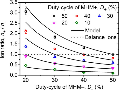
We have studied the effect of the duty-cycle combination and airflow rate on the ion production of the MHM charger. Both the MHM + and MHM– duty-cycles were varied simultaneously with several combinations at Q_ae = 1 L min⁻¹. The purpose of knowing the effect of a duty-cycle is to obtain a duty-cycle set that makes the MHM charger produce balanced ions. Moreover, we could predict the duty-cycle set so that the MHM charger could produce specific ion ratios. Figure 5 depicts the correlation between the duty-cycle and ion ratio. The ion ratio is experimentally defined as the ratio of the positive (n₊) and negative (n_–) ion concentration measured by an ion counter. A similar experimental scheme to measure ion concentration was also conducted by other researchers (Mustika et al. 2021; Kwon et al. 2005; Yun, Otani, and Emi 1997). In comparison, the ion ratio based on the calculation (n_i+/n_i–) is obtained from Equations (12)(12) $$\frac{d{n}_{g\pm }\left(t\right)}{dt}=q\left(t\right)-\alpha n_{g+}\left(t\right)n_{g-}\left(t\right)-\omega \prime n_{g\pm }\left(t\right),$$(12) and (13)(13) $$\frac{d{n}_{i\pm }\left(t^{\prime }\right)}{dt\prime }=-\alpha n_{i+}\left(t^{\prime }\right)n_{i-}\left(t^{\prime }\right),$$(13) .

Figure 5. The ratio of ion concentration in various duty-cycle configurations. The model was calculated using Equations (12)(12) $$\frac{d{n}_{g\pm }\left(t\right)}{dt}=q\left(t\right)-\alpha n_{g+}\left(t\right)n_{g-}\left(t\right)-\omega \prime n_{g\pm }\left(t\right),$$(12) and (13)(13) $$\frac{d{n}_{i\pm }\left(t^{\prime }\right)}{dt\prime }=-\alpha n_{i+}\left(t^{\prime }\right)n_{i-}\left(t^{\prime }\right),$$(13) .

Liu and Pui (1974) used an electrometer probe directly inside the ionizer chamber to obtain the ion production rate. Therefore, based on the measured saturation current, the ion production rate, q, could be determined. However, different from Liu and Pui (1974), we used an ion counter and electrometer to measure the concentration of ions (not the ion production rate) convected by the airflow drawn to the ion counter, while the ion production rate was determined indirectly.

Due to the modulation applied to both MHM ionizers, the ion production rate fluctuated. MHM HV for both MHM + and MHM– actively produced ions for T_ON (q = q₀) and did not produce ions during T_OFF (q = 0). The airflow in the aerosol charger induced ion convection, decreasing ion concentration by the rate of –n_g±/τ_g, where τ_g is the retention time inside the aerosol charger. The value of τ_g was assumed to be equal to V_eff/Q_ae (Adachi et al. 1980), where V_eff is the effective chamber volume. By considering a linear ion loss term (ω_±) due to ion-wall interactions (Franchin et al. 2015) without any aerosol particles, the ion concentration processed inside the chamber (n_g±) is determined through the following equation: (12) $$\frac{d{n}_{g\pm }\left(t\right)}{dt}=q\left(t\right)-\alpha n_{g+}\left(t\right)n_{g-}\left(t\right)-\omega \prime n_{g\pm }\left(t\right),$$(12) with $$q\left(t\right)=\{\begin{array}{c}{q}_0, \frac{t}{T_s}-\mathit{floor}\left(\frac{t}{T_s}\right)\le D_{\pm }\\ 0, \frac{t}{T_s}-\mathit{floor}\left(\frac{t}{T_s}\right)>D_{\pm }.\end{array}$$

Note that 1/τ_g is also a linear term, while assuming ω₊ = ω_– (Franchin et al. 2015), then defining ω' = 1/τ_g + ω_±. Equation (12)(12) $$\frac{d{n}_{g\pm }\left(t\right)}{dt}=q\left(t\right)-\alpha n_{g+}\left(t\right)n_{g-}\left(t\right)-\omega \prime n_{g\pm }\left(t\right),$$(12) needed to be solved first to obtain the ion concentration inside the aerosol charger as a function of time, n_g±(t). After that, the ions moved through convection toward the ion counter. Along the way, the ion concentration decayed due to recombination. By assuming that the collision of ions onto the pipe wall can be ignored (Adachi et al. 1980), the concentration of ions that reached the ion counter (n_i±) can be obtained by (13) $$\frac{d{n}_{i\pm }\left(t^{\prime }\right)}{dt\prime }=-\alpha n_{i+}\left(t^{\prime }\right)n_{i-}\left(t^{\prime }\right),$$(13) with the initial condition from the solution of Equation (12)(12) $$\frac{d{n}_{g\pm }\left(t\right)}{dt}=q\left(t\right)-\alpha n_{g+}\left(t\right)n_{g-}\left(t\right)-\omega \prime n_{g\pm }\left(t\right),$$(12) , n_i±(t' = 0) = n_g±(t). Thus, the ion concentration measured by the ion counter is n_i±(t' = τ_p), where τ_p is the retention time inside the pipeline, assumed to be τ_p = ¼ πb²L/Q_ae, where b and L are the inner diameter of the pipeline (0.4 cm) and the effective length of pipe (7.5 cm), respectively.

Considering the duty-cycle was varied and α, q₀, and ω' are unknown, the Equations (12)(12) $$\frac{d{n}_{g\pm }\left(t\right)}{dt}=q\left(t\right)-\alpha n_{g+}\left(t\right)n_{g-}\left(t\right)-\omega \prime n_{g\pm }\left(t\right),$$(12) and (13)(13) $$\frac{d{n}_{i\pm }\left(t^{\prime }\right)}{dt\prime }=-\alpha n_{i+}\left(t^{\prime }\right)n_{i-}\left(t^{\prime }\right),$$(13) cannot be solved analytically. In this article, the ion recombination rate was α = 1.6 × 10⁻⁶cm³ s⁻¹ (Hoppel and Frick 1990). The duty-cycles of both the MHM + and MHM– were varied simultaneously with the same pulse period, T_s. Meanwhile, the q₀ and ω' values were estimated by finding the best fit between the calculation and experimental results (see SI, section 3). The ion concentration was estimated in Equations (12)(12) $$\frac{d{n}_{g\pm }\left(t\right)}{dt}=q\left(t\right)-\alpha n_{g+}\left(t\right)n_{g-}\left(t\right)-\omega \prime n_{g\pm }\left(t\right),$$(12) and (13)(13) $$\frac{d{n}_{i\pm }\left(t^{\prime }\right)}{dt\prime }=-\alpha n_{i+}\left(t^{\prime }\right)n_{i-}\left(t^{\prime }\right),$$(13) using numerical calculations (the Euler method). Then, the inversion was facilitated using the least square method to determine q₀ and ω'. We found that the q₀ and ω' values were 4.62 × 10⁹ cm⁻³ s⁻¹ and 7.8 × 10² s⁻¹, respectively, with a relative root mean square error (RRMSE) of 0.32%.

Since the experimental results and the model show a significant correlation, this model could also be used to predict the ion ratio on other specific duty-cycle combinations. According to the result, the balanced ions were obtained at the duty-cycle combinations of P20N20, P30N30, P40N40, and P50N50 with ion ratios of 0.909, 0.885, 0.986, and 0.991, respectively. The possibility of controlling the ion ratio is beneficial to further application, such as controlling the charge distribution asymmetry and, notably, replicating the performance of a radioactive-based bipolar charger (Hoppel and Frick 1990). Indeed, there is more work to do to optimize and to select the set of the duty-cycles.

To study the effect of flow rate, we set the MHM charger in bipolar mode with a fixed P50N50 configuration, but various Q_ae. The experimental result is depicted in Figure 6. The concentration can be calculated using Equation (2)(2) $$n_{\pm }=\frac{|I-I_o|}{e{Q}_{ae}},$$(2) . From Figure 6, the concentrations of positive and negative ions were higher as the flow rate increased. The measurement was constrained at 1.5 L min⁻¹ because the measured ion concentration at that flow rate nearly reached the maximum limit of the electrometer (about 92% of the detection limit). The 1.75 L min⁻¹ of flow rate caused the current measured by the electrometer to reach the limit, so we did not measure the ion concentrations using this flow rate.

Figure 6. The effect of flow rate on the ion concentration produced by the MHM charger. The model was calculated using Equations (12)(12) $$\frac{d{n}_{g\pm }\left(t\right)}{dt}=q\left(t\right)-\alpha n_{g+}\left(t\right)n_{g-}\left(t\right)-\omega \prime n_{g\pm }\left(t\right),$$(12) and (13)(13) $$\frac{d{n}_{i\pm }\left(t^{\prime }\right)}{dt\prime }=-\alpha n_{i+}\left(t^{\prime }\right)n_{i-}\left(t^{\prime }\right),$$(13) .

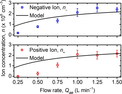
Nevertheless, from the results, we can conclude that the ion concentration will reach its asymptotic condition. Kwon et al. (2005) also found that at above 20 L min⁻¹ of flow rate, both the positive and negative ions being produced will reach their asymptotic condition. However, the experiment conducted by Mustika et al. (2021) reported that the production of ions is not monotonously increasing, but has a peak, instead. This result means that, at above a particular flow rate, the ion concentration will eventually decrease. Equations (12)(12) $$\frac{d{n}_{g\pm }\left(t\right)}{dt}=q\left(t\right)-\alpha n_{g+}\left(t\right)n_{g-}\left(t\right)-\omega \prime n_{g\pm }\left(t\right),$$(12) and (13)(13) $$\frac{d{n}_{i\pm }\left(t^{\prime }\right)}{dt\prime }=-\alpha n_{i+}\left(t^{\prime }\right)n_{i-}\left(t^{\prime }\right),$$(13) could explain the effect of the flow rate on either the monotonously increasing concentration condition or the decreasing concentration condition. The detected concentration will be zero when the flow rate is zero, since there are no ions reaching the ion counter. Therefore, when the flow rate is not zero, some ions will be drawn by the ion counter and detected as current, and the number of ions will increase as the flow rate increases. This result is due to the longer retention time in the pipeline when the flow rate is low, so the decay caused by recombination in Equation (13)(13) $$\frac{d{n}_{i\pm }\left(t^{\prime }\right)}{dt\prime }=-\alpha n_{i+}\left(t^{\prime }\right)n_{i-}\left(t^{\prime }\right),$$(13) is more dominant.

The results also show that the applied model has a trend that corresponds with the experiment, despite the difference between the model and data. However, the cause of the difference is still unidentified. By considering a sizeable retention time at low flow rates, the predominance of ion loss caused by the diffusion effect and electric field of any charge in the ionic space must be considered. Equations (12)(12) $$\frac{d{n}_{g\pm }\left(t\right)}{dt}=q\left(t\right)-\alpha n_{g+}\left(t\right)n_{g-}\left(t\right)-\omega \prime n_{g\pm }\left(t\right),$$(12) and (13)(13) $$\frac{d{n}_{i\pm }\left(t^{\prime }\right)}{dt\prime }=-\alpha n_{i+}\left(t^{\prime }\right)n_{i-}\left(t^{\prime }\right),$$(13) also show that the ion concentration will reach the plateau at a particular flow rate, and a higher flow rate will only reduce the ion concentration of the air inside the aerosol charger. There was a maximum ion concentration at a specific flow rate, Q_max. As long as the flow rate is below Q_max, the concentration will gradually increase along with the increasing flow rate until it reaches its asymptotic condition at the flow rate of Q_max and will decrease afterward. As for the calculation in this article, the developed MHM charger has Q_max = 53 L min⁻¹.

3.2. Ion mobility distribution

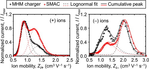
The measurement of air ion mobility produced by a charger device has been widely studied. Ungethüm (1974) observed quantized mobilities of air ions ranging from 0.26–11.2 and 0.73–11.9 cm² V⁻¹ s⁻¹ for positive and negative ions, respectively, by utilizing a fast ion spectrometer. The air ion mobilities produced by SMAC, previously examined by Kwon et al. (2005) using a high-resolution differential mobility analyzer (HR-DMA), at mobilities ranging from 0.5–2.0 and 0.7–3.0 cm² V⁻¹ s⁻¹ for positive and negative ions, respectively. Kwon et al. (2005) used multiple peaks assumption in their analyses, where the total mobility ion distribution was the accumulation of all peaks. They used lognormal fit and obtained five peaks on positive ions, which were 0.75, 0.95, 1.22, 1.47, and 1.71 cm² V⁻¹ s⁻¹ with an average value of 1.14 cm² V⁻¹ s⁻¹; as for the negative ion, they also found five peaks, which were 0.94, 1.18, 1.53, 2.01, and 2.30 cm² V⁻¹ s⁻¹, with an average value of 1.91 cm² V⁻¹ s⁻¹. We have also attempted to measure the distribution of ion mobilities produced by SMAC and the MHM charger by utilizing the mini-cyDMA. However, we only obtained two peaks for both positive and negative ions due to the limited resolution. Nonetheless, the mean of ion mobilities produced by SMAC that we obtained was in agreement with the results obtained by Kwon et al. (2005). The ion distribution produced by the MHM charger was also found to have two peaks that correspond with SMAC. The configuration of the MHM charger used in this experiment was P50N50, and the concentration ratio of positive and negative ions was equal. The measurement results are listed in Table 2.

Table 2. The air ion mobility produced by SMAC and the MHM charger with P50N50 configuration.

Ion properties	Ion source	Ion polarity
		(+)		(–)
		Mean	Median	Mean	Median
Peak 1 (cm^2 V^-1 s^-1)	SMAC	0.880	0.872	1.432	1.399
	MHM	0.931	0.919	1.348	1.311
Peak 2 (cm^2 V^-1 s^-1)	SMAC	1.297	1.280	2.121	2.108
	MHM	1.384	1.373	2.056	2.045
Mean mobility (cm^2 V^-1 s^-1)	SMAC	1.140		1.910
	MHM	1.090		1.670
Ion concentration (cm^-3)	SMAC	2.15 × 10^6		2.27 × 10^6
	MHM	2.45 × 10^6		2.47 × 10^6
Diffusion coefficient (m^2 s^-1)	SMAC	2.96 × 10^-6		4.95 × 10^-6
	MHM	2.83 × 10^-6		4.33 × 10^-6.

As shown in Figure 7, the ions produced by both SMAC and the MHM charger are distributed at the same peak, peak 1 and peak 2. However, the intensity ratio of peak 1 to peak 2 for both the positive and negative ions of the MHM charger is higher than that of SMAC. Thus, the mean positive ion mobilities produced by the MHM charger are less than those of SMAC, 1.09 and 1.14 cm² V⁻¹ s⁻¹, respectively. The mean negative ion mobilities produced by the MHM charger are also smaller than those of SMAC, which are 1.67 and 1.91 cm² V⁻¹ s⁻¹, respectively. As a result, the ratio of the mean mobility of positive and negative ions produced by SMAC and the MHM charger are 0.597 and 0.653, respectively. A similar value of ion mobility ratio produced by SMAC was previously obtained by Kwon et al. (2005). In other previous measurements, with a different charger, the ion mobility ratios obtained by Adachi, Kousaka, and Okuyama (1985), Hussin et al. (1983), and Wiedensohler et al. (1986) were 0.737, 0.827, and 0.844, respectively. Diffusivity of the produced ions can be determined by a quantity called the diffusion coefficient (D_ion±) and calculated using the equation provided by Adachi, Kousaka, and Okuyama (1985), as follows: (14) $$D_{\mathit{ion}\pm }=\frac{kT{Z}_{i\pm }}{e},$$(14) where k and T are Boltzmann’s coefficient and absolute temperature, respectively. SMAC and the MHM charger have similar peak mobility, but the diffusion coefficient of the MHM charger is smaller than that of SMAC due to the difference between the peak intensities.

Figure 7. The distribution of positive and negative air ions induced by SMAC and the MHM charger with peak analysis data obtained through the lognormal distribution function.

3.3. Particle generation

One of the corona-based charger issues was the presence of new particles generated due to sputtering or chemical reactions (Romay, Liu, and Pui 1994). In SMAC developed by Kwon et al. (2006), the generated particle was detected when the particle was sized at less than 20 nm and marked by a charged particle penetration ratio, r_c, at more than 1. In this research, generated particles with a size of more than 20 nm were not found in the MHM charger and SMAC. Hence, in this article, we directly measured the generated particle concentration using CPC3025, as shown in Figure 4a. When the chargers (either the SMAC or the MHM charger) were in the OFF condition, there were no particles detected by CPC3025, which means no leakage in the system. However, in the ON condition, there were particles detected by CPC3025, which means that the sputtering electrode generated the particles. The result implied that the SMAC and the MHM charger are consistent in generating particles having an average concentration of 8.6 and 5.2 cm⁻³, respectively. Therefore, the average generated particle concentration of the MHM charger is lower than that of SMAC.

3.4. Particle penetration ratio

It is well known that there are two kinds of particle losses, namely, flow loss and electrostatic loss, caused by mechanical deposition (diffusion, impaction, or interception particle by aerosol flow) and by electrical precipitation (by electrostatic force), respectively (Yu et al. 2017). We examined the penetration of particles under two conditions, namely, particles that are initially neutral and charged. The purpose of observing the penetration ratio using neutral and charged particle sources is to examine the particle loss caused by mechanical deposition and electrical precipitation.

The particle penetration ratio, which we call the charged particle penetration ratio (r_c), was studied by Kwon et al. (2006) to characterize the total particle loss (caused by both electrical precipitation and mechanical deposition) inside SMAC when the inlet particles were initially charged. Kwon et al. (2006) found that the charged particle penetration ratios within the range of 20–200 nm were above 0.9 and had an average of 0.96 in the range of 25–100 nm. We have conducted a measurement using SMAC and found that the average charged particle penetration ratio in the range of 25–100 nm was 0.9, which is slightly less than the one found by Kwon et al. (2006) (see Figure 8). The difference might be due to the discrepancy of SMAC + and SMAC– placement configuration inside the chamber. They used a dual-electrode configuration on each chamber lid, while we used a single electrode configuration. Thus, the electrical field distribution within the chamber in this study was different from that of their studies. A dual-electrode configuration gives a smaller field compared with a single electrode configuration and leads to a lower precipitation effect.

Figure 8. The charged particle penetration ratios of SMAC and the MHM charger (measured using the experimental setup in Figure 4b and calculated using Equation (3)(1) $$D_{\pm }=\frac{T_{\mathrm{ON}\pm }}{T_s}\times 100\%,$$(1) ) compared with the previous study of SMAC by Kwon et al. (2006).

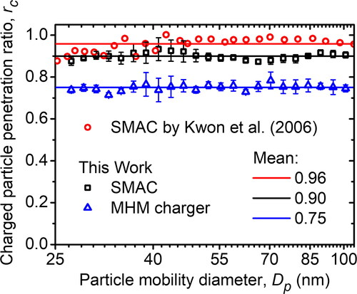
Furthermore, we measured the charged particle penetration ratio of the MHM charger with P50N50 configuration. The experimental results show that the average charged particle penetration ratio is 0.75, which is much smaller than that of SMAC. The results are depicted in Figure 8. Because the discharge mode of the MHM charger is VD, the gap between electrodes is quite large compared with the gap in SD, so many charged particles are easily attracted to the electrodes. Also, the MHM electrode structure enables turbulence formation due to the electro-hydrodynamic effect (Guan et al. 2018; Davidson and Shaughnessy 1986).

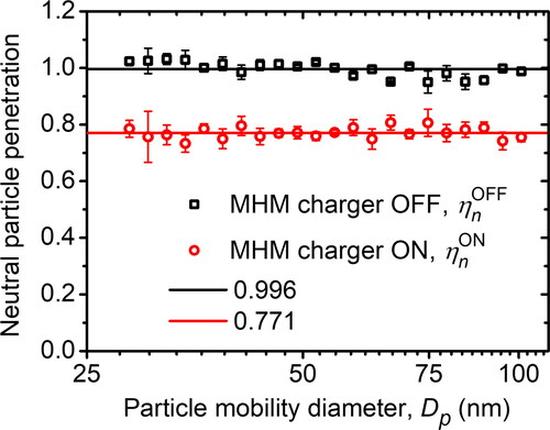
We characterized the particle penetration of the MHM charger when the inlet particle was in the neutral condition. The results are depicted in Figure 9. We obtained the average neutral particle penetration when the MHM charger was OFF (η_n^OFF) and ON (η_n^ON), at a 25–100 nm range, were 0.996 and 0.771, respectively. As a result, the average neutral-particle penetration ratio (r_n) was 0.774. The particle penetration obtained when the MHM charger was OFF, which was 1 – η_n^OFF = 0.4%, can be used to study the particle loss caused by mechanical deposition on the charger. Additionally, the particle penetration obtained when the MHM was ON can be used to determine the total particle loss using 1 – η_n^ON = 22.9%, whereas particle loss caused only by electrical precipitation was determined by (η_n^OFF – η_n^ON)/η_n^OFF = 22.6% (Yu et al. 2017). This result indicates that the particle loss caused by electrical precipitation is more dominant than the particle loss caused by mechanical deposition. The fact that particle loss due to electrical precipitation is more dominant than due to mechanical deposition implies that the corona-discharge-based charger has a short lifetime. For long-term use (more than 120 h of use as a charger in an MPG setup), other than depositing on the walls and the area around the electrodes, we also found that particles deposited on the electrode, where these impurities might affect the micro discharge state (see Figure S5). Hence, the electrode needs to be cleaned regularly for continuous usage. In general, the corona discharge-type charger used sheath air (Stommel and Riebel 2004; Romay, Liu, and Pui 1994).

Figure 9. The neutral particle penetration of the MHM charger calculated in Equations (4)(2) $$n_{\pm }=\frac{|I-I_o|}{e{Q}_{ae}},$$(2) and (5)(11) $$f_0^{\prime }=\frac{N_4^{\mathrm{ON}}}{\frac{{\xi }_n^{\mathrm{OFF}}}{{\xi }_c^{\mathrm{OFF}}{r}_c}{N}_4^{\mathrm{OFF}}+\left(1-\frac{{\xi }_n^{\mathrm{OFF}}}{{\xi }_c^{\mathrm{OFF}}}\right)N_4^{\mathrm{ON}}}.$$(11) and measured using the experimental setup in Figure 4c.

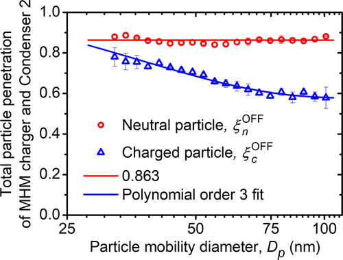
Besides measuring the particle penetration, we also measured the total particle penetration of the MHM charger and Condenser 2, as shown in Figure 4d. The measurement was done using a neutral- and charged-particle inlet. This experiment aimed to observe the total particle loss in the MHM charger and Condenser 2 so it could be used to correct the neutral fraction in Equation (9). The results are shown in Figure 10. We found that the total neutral particle penetration of the MHM charger and Condenser 2 (ξ_n^OFF) was 0.863. Since the neutral particle penetration of the MHM was almost 1, it is understandable that the particle loss due to deposition in Condenser 2 was fairly large. The neutral particle loss in Condenser 2 was (η_n^OFF – ξ_n^OFF)/η_n^OFF = 13.35%. However, the charged particle penetration was found to be diameter dependent, as Alonso and Alguacil (2003) and Alonso et al. (1997a) also observed. Charged particle–wall interactions in condensers and other loss mechanisms also affect penetration (Franchin et al. 2015). According to the explanation, we believed that the charged particles were larger and easily deposited in Condenser 2. We then applied third-order polynomial fitting to the charged particle and mobility diameter relationship. The electrical precipitation effect caused the charged particle penetration to constantly be lower than the neutral particle penetration, as shown in Figures 8–10. The charged particles tend to stick to the wall more easily due to the electrostatic force of the charge itself. In contrast, the neutral particles are solely deposited only due to mechanical deposition. During the measurement, when Condenser 2 was in the OFF condition, both parallel plates of the condenser were grounded to ensure there was no static charge. It is well known that static charge could cause the deposition to become very unpredictable and could bias the measurement data. Therefore, we attempted triplicate measurements of ξ_n^OFF and ξ_c^OFF. The results showed quite a good repeatability, indicated by a relatively small error bar.

Figure 10. The total penetration of neutral and charged particles of the MHM-Condenser 2 calculated in Equations (6)(12) $$\frac{d{n}_{g\pm }\left(t\right)}{dt}=q\left(t\right)-\alpha n_{g+}\left(t\right)n_{g-}\left(t\right)-\omega \prime n_{g\pm }\left(t\right),$$(12) and (7)(13) $$\frac{d{n}_{i\pm }\left(t^{\prime }\right)}{dt\prime }=-\alpha n_{i+}\left(t^{\prime }\right)n_{i-}\left(t^{\prime }\right),$$(13) and measured using the experimental setup in Figure 4d. The third-order polynomial fit was applied to the total penetration of charged particles.

3.5. Charging probability

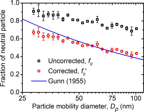
The neutral particle fraction, f₀, was measured through the experimental setup shown in Figure 4d. The neutral particles generated using the MPG-SMAC-Condenser 1 configuration were utilized to characterize the MHM charger. In this experiment, Condenser 2 worked to remove the charged particles to obtain neutral particle concentration. The neutral fraction results are depicted in Figure 11. The calculated values of Equation (8), which included particle loss correction in Equation (11)(11) $$f_0^{\prime }=\frac{N_4^{\mathrm{ON}}}{\frac{{\xi }_n^{\mathrm{OFF}}}{{\xi }_c^{\mathrm{OFF}}{r}_c}{N}_4^{\mathrm{OFF}}+\left(1-\frac{{\xi }_n^{\mathrm{OFF}}}{{\xi }_c^{\mathrm{OFF}}}\right)N_4^{\mathrm{ON}}}.$$(11) , were denoted by a black square (□) and a red round (○) symbol. The result was compared to the theoretically predicted values studied by Gunn (1955), with an ion concentration ratio (n₊/n_–) and ion mobility ratio (Z_i+/Z_i–) of 0.992 and 0.653, respectively. The result of the experiment is in accordance with the predicted values. However, the calculations without the particle loss correction and the predicted value were not in accordance. This is because the particle loss in Condenser 2 was significant. The neutral fraction obtained experimentally and the predicted value decreased as the particle size increased, indicating that the large particle has a more significant probability of being charged because the large limiting sphere contains more ions. However, this article cannot provide a comprehensive review of individual charge states due to practical constraints.

Figure 11. The corrected fraction of neutral particles obtained by the MHM charger compared with the uncorrected value and the calculation model proposed by Gunn (1955), with an ion concentration ratio and ion mobility ratio of 0.992 and 0.653, respectively.

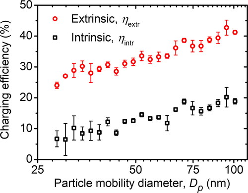
Besides neutral fraction and charged particle fraction, another critical characteristic of a charger is charging efficiency, primarily extrinsic charging efficiency. The extrinsic charging efficiency (η_extr) involves both diffusional loss and electrostatic loss, while the intrinsic charging efficiency (η_intr) only involves diffusional loss. Accordingly, a highly efficient charger design usually minimizes the charged particle loss by controlling ion transport and particle transport inside the chamber (Manirakiza et al. 2013). Other than geometry, the voltage source used by the corona discharge has a considerable impact too. For instance, Kwon, Sakurai, and Seto (2007) used DC pulses and found that the extrinsic charging efficiency was 25% at a particle size of 10.5 nm. Moreover, Manirakiza et al. (2013) improved the extrinsic charging efficiency to 66.7% by using an HV source of Sinc waveform.

In this research, we also studied the intrinsic and extrinsic charging efficiencies of the MHM charger. As depicted in Figure 12, the charging efficiencies increased as the particle size increased. This is due to the decreasing neutral fraction as the particle size increases, as shown in Figure 11. A significant difference between intrinsic and extrinsic charging efficiency indicates a large number of particle losses. As mentioned before, the particle penetration ratio of the MHM charger for initially charged or neutral particles, which were 0.75 and 0.774, was smaller than that of SMAC. However, we could improve the charging efficiency of the MHM charger using sheath air. Figure 1 depicts a comprehensive schematic of the MHM charger with a sheath air Q_cr. The use of sheath air in the MHM charger will be discussed fully in future works.

Figure 12. The intrinsic and extrinsic charging efficiencies of the MHM charger calculated in Equations (9)(14) $$D_{\mathit{ion}\pm }=\frac{kT{Z}_{i\pm }}{e},$$(14) and (10)(14) $$D_{\mathit{ion}\pm }=\frac{kT{Z}_{i\pm }}{e},$$(14) and measured using the experimental setup in Figure 4d.

3.6. Particle electrical mobility distribution

Typically, size distribution measurement utilizing a DMA used a radioactive source as the neutralizer. However, because the radioactive source has some limitations, various charger types have been developed as a neutralizer substitute. Kwon et al. (2005) developed a SMAC that could be used as a charger to measure particle mobility and had a similar measurement result compared to using a ²⁴¹Am neutralizer. Moreover, Stommel and Riebel (2004) established an electrical-neutralizer-based corona discharge using ⁸⁵Kr as a comparison. In our research, the next step after we characterized the charging probability of the MHM charger was to implement it as a possible replacement for the radioactive source. We measured and compared the result with the one obtained by SMAC, as depicted in Figure 13.

Figure 13. The particle mobility distributions of negatively charged particles obtained by SMAC and the MHM charger using the experimental setup in Figure 4c.

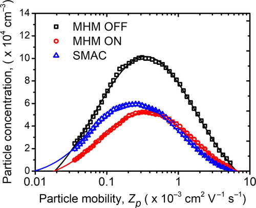
The result shows a slight difference in the particle concentrations and measured particle mobility peaks between the MHM and SMAC. The particle mobility peaks of SMAC, MHM ON, and MHM OFF are 0.50 × 10⁻³, 0.58 × 10⁻³, and 0.58 × 10⁻³ cm² V⁻¹ s⁻¹, respectively. The MHM charger in the ON condition has the same particle mobility peaks as in the particle distribution without the neutralizer (MHM charger in OFF condition). In this case, the MHM charger only neutralized the particle, whereas its effect on charging low-mobility particles was barely observable. In contrast, SMAC was able to shift the particle mobility peak to the left. This implies that SMAC could reduce multicharge on particles caused by contact charging through solution atomization (Kwon et al. 2005). Nevertheless, the number of multicharged particles caused by contact charging during the atomization process was minimized by using the solution with a high molar concentration (Forsyth, Liu, and Romay 1998).

4. Conclusions

A bipolar charger has been developed by utilizing commercially available ionizer modules (Model MHM 305-1 and 400-1, Murata Manufacturing Co., Ltd., Japan). A cheap commercial ionizer was used to make the setup simple and easily replicated because of its consistent characteristics. A simple HV driver has been made to regulate ion production (adjustable ion ratio). The adjustable ion ratio is beneficial. For instance, if we balance the ion concentration, it could replicate the performance of the radioactive ionizer. Moreover, it could regulate the symmetry of the charge distribution when we set it to any particular ion concentration.

We examined the ion production concentration against duty-cycle and flow rate variation, ion mobility distribution, particle generation, particle penetration, and the charging probability of the MHM charger. The results show that positive and negative ion production ratios can be regulated by adjusting the duty-cycle configuration. Meanwhile, the flow rate has an impact on the quantity of ion concentration. At flow rates of 0.5–1.5 L min⁻¹, the concentration increased as the flow rate increased.

We obtained two peaks for each positive and negative ion distribution. For positive ion distribution, the observed peaks were 0.9 and 1.35 cm² V⁻¹ s⁻¹, with an average of 1.09 cm² V⁻¹ s⁻¹. While for the negative ion distribution, the peaks were 1.24 and 2.03 cm² V⁻¹ s⁻¹, with an average of 1.67 cm² V⁻¹ s⁻¹. The particle penetration of the MHM charger is still lower than that of SMAC. We have also investigated the issue of new particle formation due to sputtering. The average generated particle concentration of the MHM charger is lower than that of SMAC, which are 5.2 and 8.6 cm⁻³, respectively.

The neutral fraction measured by the MHM charger has an acceptable fit to the given prediction model. Also, we have observed the particle penetration with initially charged and neutral particles along with the intrinsic and extrinsic charging efficiencies. The intrinsic and extrinsic charging efficiencies were above 6% and 20% at a range of 20–100 nm, respectively. The efficiencies tended to increase as the particle size increased by approximately 19% and 41% at 100 nm, respectively. Also, we studied the implementation of the MHM charger as a neutralizer in a monodisperse particle generator system. We compared the performance of the MHM charger to SMAC, and the results show that the MHM charger can be used as an alternative aerosol charger without using radioactive sources.

Acknowledgments

C.S. gratefully acknowledges the Minister of Education, Culture, Research and Technology Indonesia for the provision of a master leading to doctoral scholarship (PMDSU). The authors thank Prof. Kikuo Okuyama and Prof. Takafumi Seto for providing LDMA and SMAC apparatus.

Additional information

Funding

This research was financially supported by Institut Teknologi Bandung (ITB) Research Grant (74/IT1.C02/TA.00/2021) in the fiscal year of 2021 and the University’s Excellence Applied Research (PTUPT) Grant in the fiscal years of 2020–2022.

Notes

1 Government regulation of the Republic of Indonesia number 29 of 2008.

Appendix

A1. Particle loss inside the charger

Yu et al. (2017) defined the particle loss caused by mechanical deposition (L_d) as (A1) $$L_d=\frac{N_0^n-N_2^{\mathit{OFF}}}{N_0^n}=1-{\eta }_n^{\mathit{OFF}}.$$(A1)

In addition, the total particle loss (L) could be determined through (A2) $$L=\frac{N_0^n-N_2^{ON}}{N_0^n}=1-{\eta }_n^{ON}.$$(A2)

Therefore, we could calculate particle losses only due to electrical precipitation (L_e), using (A3) $$L_e=\frac{N_2^{\mathit{OFF}}-N_2^{ON}}{N_2^{\mathit{OFF}}}=\frac{{\eta }_n^{\mathit{OFF}}-{\eta }_n^{ON}}{{\eta }_n^{\mathit{OFF}}}.$$(A3)

A2. Particle loss inside Condenser 2

The total neutral particle penetration of the MHM charger and Condenser 2 was defined in Equation (6)(1) $$D_{\pm }=\frac{T_{\mathrm{ON}\pm }}{T_s}\times 100\%,$$(1) . The neutral particle loss only in Condenser 2 (L_cd) could be calculated using $$L_{cd}=\frac{N_3^n-N_4^{\mathit{OFF}}}{N_3^n},$$ where N₃ⁿ is the particle concentration at the downstream of the MHM charger in the OFF condition. Remember that N₃ⁿ/N₀ⁿ is equal to N₂°^FF/N₀ⁿ; therefore, (A4) $$L_{cd}=\frac{N_2^{\mathit{OFF}}/N_0^n-N_4^{\mathit{OFF}}/N_0^n}{N_2^{\mathit{OFF}}/N_0^n}= \frac{{\eta }_n^{\mathit{OFF}}-{\xi }_n^{\mathit{OFF}}}{{\eta }_n^{\mathit{OFF}}}.$$(A4)

The total charged particle penetration of the MHM charger and Condenser 2 was defined in Equation (7)(A7) $$N_4^{ON}={\xi }_n^{ON}{N}_n={\xi }_n^{\mathit{OFF}}{N}_n,$$(A7) . The charged particle loss only in Condenser 2 (L_ce) could be calculated as $$L_{ce}=\frac{N_3^c-N_4^{\mathit{OFF}}}{N_3^c}.$$

Note that N₃ⁿ is equal to N₂^OFF; therefore, (A5) $$L_{ce}=\frac{N_2^{ON}-N_4^{\mathit{OFF}}}{N_2^{ON}}= \frac{{\eta }_c^{\mathit{OFF}}-{\xi }_c^{\mathit{OFF}}}{{\eta }_c^{\mathit{OFF}}},$$(A5) where η_c^OFF is defined as N₂^ON/N₀^c.

A3. Neutral fraction correction by considering particle loss

Kwon et al. (2006) measured neutral fraction as the ratio of particle concentration at the downstream of Condenser 2 when Condenser 2 was in the ON and OFF condition. When Condenser 2 was in the ON condition, the system only measured neutral particles since the charged particles were trapped in Condenser 2. When Condenser 2 was in the OFF condition, it would measure the total of neutral and charged particles. Therefore, the neutral fraction could be calculated through Equation (8). However, this approximation neglects the particle loss in either the MHM charger or Condenser 2. The neutral particle concentration at the upstream MHM charger is N₀ⁿ. Ideally, the total particle concentration at the downstream of the MHM charger remains the same, so the particle concentration that has been charged (N_c) and the concentration of the remaining neutral particle (N_n) is N_c + N_n = N₀ⁿ. Hence, the neutral fraction without particle loss (namely, f₀′) should be defined as (A6) $$f_0^{\prime }=\frac{N_n}{N_c+N_n}.$$(A6)

However, neither N_c or N_n, could be measured directly. The experimental setup in Figure 4d shows the particle measurement after the particles went through the MHM charger and Condenser 2. As for the detected neutral particle, N₄^ON can be considered to be N_n that has been deposited partially. Therefore, the relation between N₄^ON and N_n can be approximated using (A7) $$N_4^{ON}={\xi }_n^{ON}{N}_n={\xi }_n^{\mathit{OFF}}{N}_n,$$(A7) where ξ_n^ON is the total penetration of the neutral particle of the MHM charger and Condenser 2 when Condenser 2 is in the ON condition. This parameter was not measured, but since the particle is neutral, we could assume that ξ_n^ON = ξ_n^OFF. However, N₄^OFF consists of neutral and charged particles. We know that the charged particle and neutral particle have different penetration, so N₄^OFF can be obtained through (A8) $$N_4^{\mathit{OFF}}={\xi }_n^{\mathit{OFF}}{N}_n+{\eta }_c^{ON}\left(1-L_{ce}\right)N_c,$$(A8) where 1 – L_ce is the charged particle penetration of Condenser 2 when it was in the OFF condition. η_c^ON is the charged particle penetration of the MHM charger when it was in the ON condition. Therefore, η_c^ON(1 – L_ce) is the total penetration where the MHM charger and Condenser 2 conditions were in the ON and OFF conditions, respectively. Considering that η_n^ON(1 – L_ce) = η_c^ON ξ_c^OFF/η_c^OFF and knowing that η_c^ON/η_c^OFF is the ratio of charged particle penetration, r_c = η_c^ON/η_c^OFF. Thus, by substituting Equations (A7)(A7) $$N_4^{ON}={\xi }_n^{ON}{N}_n={\xi }_n^{\mathit{OFF}}{N}_n,$$(A7) and (A8)(A8) $$N_4^{\mathit{OFF}}={\xi }_n^{\mathit{OFF}}{N}_n+{\eta }_c^{ON}\left(1-L_{ce}\right)N_c,$$(A8) into Equation (A6)(A6) $$f_0^{\prime }=\frac{N_n}{N_c+N_n}.$$(A6) , we will get the following formula: (A9) $$f_0^{\prime }=\frac{N_4^{\mathrm{ON}}}{\frac{{\xi }_n^{\mathrm{OFF}}}{{\xi }_c^{\mathrm{OFF}}{r}_c}{N}_4^{\mathrm{OFF}}+\left(1-\frac{{\xi }_n^{\mathrm{OFF}}}{{\xi }_c^{\mathrm{OFF}}}\right)N_4^{\mathrm{ON}}}.$$(A9)

References

- Adachi, M., Y. Kousaka, and K. Okuyama. 1985. Unipolar and bipolar diffusion charging of ultrafine aerosol particles. J. Aerosol Sci. 16 (2):109–23. doi:10.1016/0021-8502(85)90079-5.
- Adachi, M., K. Okuyama, Y. Kousaka, and T. Takahashi. 1980. Electrical charging of uncharged aerosol particles under at bipolar ion concentrations. J. Chem. Eng. Japan. 13 (1):55–60. doi:10.1252/jcej.13.55.
- Alonso, M., and F. J. Alguacil. 2003. The effect of ion and particle losses in a diffusion charger on reaching a stationary charge distribution. J. Aerosol Sci. 34 (12):1647–64. doi:10.1016/S0021-8502(03)00357-4.
- Alonso, M., Y. Kousaka, T. Hashimoto, and N. Hashimoto. 1997a. Penetration of nanometer-sized aerosol particles through wire screen and laminar flow tube. Aerosol Sci. Technol. 27 (4):471–80. doi:10.1080/02786829708965487.
- Alonso, M., Y. Kousaka, T. Nomura, N. Hashimoto, and T. Hashimoto. 1997b. Bipolar charging and neutralization of nanometer-sized aerosol particles. J. Aerosol Sci. 28 (8):1479–90. doi:10.1016/S0021-8502(97)00036-0.
- Barmpounis, K., A. Maisser, A. Schmidt-Ott, and G. Biskos. 2016. Lightweight differential mobility analyzers: Toward new and inexpensive manufacturing methods. Aerosol Sci. Technol. 50 (1):2–5. doi:10.1080/02786826.2015.1130216.
- Cai, R., D.-R. Chen, J. Hao, and J. Jiang. 2017. A miniature cylindrical differential mobility analyzer for sub-3 nm particle sizing. J. Aerosol Sci. 106:111–9. doi:10.1016/j.jaerosci.2017.01.004.
- Clement, C. F., and R. G. Harrison. 1992. The charging of radioactive aerosols. J. Aerosol Sci. 23 (5):481–504. doi:10.1016/0021-8502(92)90019-R.
- Davidson, J. H., and E. J. Shaughnessy. 1986. Turbulence generation by electric body forces. Exp. Fluids 4 (1):17–26. doi:10.1007/BF00316781.
- Forsyth, B., B. Y. H. Liu, and F. J. Romay. 1998. Particle charge distribution measurement for commonly generated laboratory aerosols. Aerosol Sci. Technol. 28 (6):489–501. doi:10.1080/02786829808965540.
- Franchin, A., S. Ehrhart, J. Leppä, T. Nieminen, S. Gagné, S. Schobesberger, D. Wimmer, J. Duplissy, F. Riccobono, E. M. Dunne, et al. 2015. Experimental investigation of ion–ion recombination under atmospheric conditions. Atmos. Chem. Phys. 15 (13):7203–16. doi:10.5194/acp-15-7203-2015.
- Gibalov, V. I., and G. J. Pietsch. 2000. The development of dielectric barrier discharges in gas gaps and on surfaces. J. Phys. D. Appl. Phys. 33 (20):2618–36. doi:10.1088/0022-3727/33/20/315.
- Guan, Y., R. S. Vaddi, A. Aliseda, and I. Novosselov. 2018. Analytical model of electro-hydrodynamic flow in corona discharge. Phys. Plasmas 25 (8):83507.
- Gunn, R. 1955. The statistical electrification of aerosols by ionic diffusion. J. Colloid Sci. 10 (1):107–19. doi:10.1016/0095-8522(55)90081-7.
- Hernandez-Sierra, A., F. J. Alguacil, and M. Alonso. 2003. Unipolar charging of nanometer aerosol particles in a corona ionizer. J. Aerosol Sci. 34 (6):733–45. doi:10.1016/S0021-8502(03)00033-8.
- Hontañón, E., and F. E. Kruis. 2008. Single charging of nanoparticles by UV photoionization at high flow rates. Aerosol Sci. Technol. 42 (4):310–23. doi:10.1080/02786820802054244.
- Hoppel, W. A., and G. M. Frick. 1990. The nonequilibrium character of the aerosol charge distributions produced by neutralizes. Aerosol Sci. Technol. 12 (3):471–96. doi:10.1080/02786829008959363.
- Hussin, A., H. G. Scheibel, K. H. Becker, and J. Porstendörfer. 1983. Bipolar diffusion charging of aerosol particles—I: Experimental results within the diameter range 4–30 nm. J. Aerosol Sci. 14 (5):671–7. doi:10.1016/0021-8502(83)90071-X.
- IAEA. 2005. Categorization of radioactive sources IAEA safety standards series no. RS-G-1.9. IAEA. Saf. Guid. 70: 7–10.
- Ibarra, I., J. Rodríguez-Maroto, and M. Alonso. 2020. Bipolar charging and neutralization of particles below 10 nm, the conditions to reach the stationary charge distribution, and the effect of a non-stationary charge distribution on particle sizing. J. Aerosol Sci. 140:105479. doi:10.1016/j.jaerosci.2019.105479.
- Intra, P., and N. Tippayawong. 2009. Measurements of ion current from a corona-needle using a faraday cup electrometer. Chiang Mai J. Sci. 36 (1):110–9.
- Kimoto, S., K. Mizota, M. Kanamaru, H. Okuda, D. Okuda, and M. Adachi. 2009. Aerosol charge neutralization by a mixing-type bipolar charger using corona discharge at high pressure. Aerosol Sci. Technol. 43 (9):872–80. doi:10.1080/02786820902998381.
- Kimoto, S., K. Saiki, M. Kanamaru, and M. Adachi. 2010. A small mixing-type unipolar charger (SMUC) for nanoparticles. Aerosol Sci. Technol. 44 (10):872–80. doi:10.1080/02786826.2010.498796.
- Kruis, F. E., and H. Fissan. 2001. Nanoparticle charging in a twin hewitt charger. J. Nanoparticle Res. 3 (1):39–50. doi:10.1023/A:1011425816983.
- Kwon, S.-B., H. Sakurai, and T. Seto. 2007. Unipolar charging of nanoparticles by the surface-discharge microplasma aerosol charger (SMAC). J. Nanopart. Res. 9 (4):621–30. doi:10.1007/s11051-006-9117-2.
- Kwon, S. B., T. Fujimoto, Y. Kuga, H. Sakurai, and T. Seto. 2005. Characteristics of Aerosol charge distribution by surface-discharge microplasma aerosol charger (SMAC). Aerosol Sci. Technol. 39 (10):987–1001. doi:10.1080/02786820500380263.
- Kwon, S. B., H. Sakurai, T. Seto, and Y. J. Kim. 2006. Charge neutralization of submicron aerosols using surface-discharge microplasma. J. Aerosol Sci. 37 (4):483–99. doi:10.1016/j.jaerosci.2005.05.007.
- Li, L., and D.-R. Chen. 2011. Performance study of a DC-corona-based particle charger for charge conditioning. J. Aerosol Sci. 42 (2):87–99. doi:10.1016/j.jaerosci.2010.12.001.
- Liu, B. Y. H., and D. Y. H. Pui. 1974. Electrical neutralization of aerosols. J. Aerosol Sci. 5 (5):465–72. doi:10.1016/0021-8502(74)90086-X.
- Liu, B. Y. H., D. Y. H. Pui, and B. Y. Lin. 1986. Aerosol charge neutralization by a radioactive alpha source. Part. Part. Syst. Charact. 3 (3):111–6. doi:10.1002/ppsc.19860030304.
- Liu, S., and M. Neiger. 2001. Excitation of dielectric barrier discharges by unipolar submicrosecond square pulses. J. Phys. D. Appl. Phys. 34 (11):1632–8. doi:10.1088/0022-3727/34/11/312.
- Manirakiza, E., T. Seto, S. Osone, K. Fukumori, and Y. Otani. 2013. High-efficiency unipolar charger for sub-10 nm aerosol particles using surface-discharge microplasma with a voltage of sinc function. Aerosol Sci. Technol. 47 (1):60–8. doi:10.1080/02786826.2012.725492.
- Munir, M. M., A. Suhendi, T. Ogi, F. Iskandar, and K. Okuyama. 2013. Ion-induced nucleation rate measurement in SO2/H 2O/N2 gas mixture by soft X-ray ionization at various pressures and temperatures. Adv. Powder Technol. 24 (1):143–9. doi:10.1016/j.apt.2012.04.002.
- Mustika, W. S., D. A. Hapidin, C. Saputra, and M. M. Munir. 2021. Dual needle corona discharge to generate stable bipolar ion for neutralizing electrosprayed nanoparticles. Adv. Powder Technol. 32 (1):166–74. doi:10.1016/j.apt.2020.11.026.
- Nishida, R. T., A. M. Boies, and S. Hochgreb. 2018. Measuring ultrafine aerosols by direct photoionization and charge capture in continuous flow. Aerosol Sci. Technol. 52 (5):546–56. doi:10.1080/02786826.2018.1430350.
- Nishida, R. T., T. J. Johnson, J. S. Hassim, B. M. Graves, A. M. Boies, and S. Hochgreb. 2020. A simple method for measuring fine-to-ultrafine aerosols using bipolar charge equilibrium. ACS Sens. 5 (2):447–53. doi:10.1021/acssensors.9b02143.
- Okuyama, K., N. Kitada, and T. Motouchi. 1983. Bipolar charging of ultrafine aerosol particles. Aerosol Sci. Technol. 2 (4):421–7.
- Osone, S., E. Manirakiza, T. Seto, Y. Otani, and T. Fujimoto. 2012. Potential of surface-discharge microplasma device as ion source for high-efficiency electrical charging of nanoparticles. J. Chem. Eng. Japan. 45 (1):21–7. doi:10.1252/jcej.11we135.
- Qi, C., and P. Kulkarni. 2013. Miniature dual-corona ionizer for bipolar charging of aerosol. Aerosol Sci. Technol. 47 (1):81–92.
- Romay, F. J., B. Y. H. Liu, and D. Y. H. Pui. 1994. A sonic jet corona ionizer for electrostatic discharge and aerosol neutralization. Aerosol Sci. Technol. 20 (1):31–41. doi:10.1080/02786829408959661.
- Shimada, M., B. Han, K. Okuyama, and Y. Otani. 2002. Bipolar charging of aerosol nanoparticles by a soft x-ray photoionizer. J. Chem. Eng. Japan. 35 (8):786–93. doi:10.1252/jcej.35.786.
- Song, D. K., H. M. Lee, H. Chang, S. S. Kim, M. Shimada, and K. Okuyama. 2006. Performance evaluation of long differential mobility analyzer (LDMA) in measurements of nanoparticles. J. Aerosol Sci. 37 (5):598–615. doi:10.1016/j.jaerosci.2005.06.003.
- Stommel, Y. G., and U. Riebel. 2004. A new corona discharge-based aerosol charger for submicron particles with low initial charge. J. Aerosol Sci. 35 (9):1051–69. doi:10.1016/j.jaerosci.2004.03.005.
- Ungethüm, E. 1974. The mobilities of small ions in the atmosphere and their relationship. J. Aerosol Sci. 5 (1):25–37. doi:10.1016/0021-8502(74)90004-4.
- Whitby, K. T. 1961. Generator for producing high concentrations of small ions. Rev. Sci. Instrum. 32 (12):1351–5. doi:10.1063/1.1717250.
- Wiedensohler, A., E. Lütkemeier, M. Feldpausch, and C. Helsper. 1986. Investigation of the bipolar charge distribution at various gas conditions. J. Aerosol Sci. 17 (3):413–6. doi:10.1016/0021-8502(86)90118-7.
- Yu, T., Y. Yang, J. Liu, H. Gui, J. Zhang, Y. Cheng, W. Wang, P. Du, J. Wang, and H. Wang. 2017. Comparative study of cylindrical and parallel-plate electrophoretic separations for the removal of ions and sub-23 nm particles. J. Sep. Sci. 40 (24):4813–24. doi:10.1002/jssc.201700750.
- Yun, C.-M., Y. Otani, and H. Emi. 1997. Development of unipolar ion generator—separation of ions in axial direction of flow. Aerosol Sci. Technol. 26 (5):389–97. doi:10.1080/02786829708965439.