Design and experimental setup of a new concept of an aerosol-on-demand print head

Abstract

Aerosol jet printing is an alternative to inkjet printing, the currently most established fabrication technique for printed electronics, with the benefits of small feature sizes, more homogeneous thickness of the printed layers, and the possibility to print on 3D structures. Printers are available on the market, in which the aerosol is generated outside of the print heads, with the disadvantage that only continuous operation is possible due to the long distance between atomization unit and print head. We report on the development and validation of a new integrated principle, with the atomization of the ink directly inside the print head. This enables a compact design, printing in all spatial directions and jet-on-demand operation. Based on fluid dynamic simulations, an optimized integrated print head design was developed, and fabricated. First tests have been performed in a preliminary laboratory test setup. The successful focusing of the aerosol to approximately 1/7 of the spread of the non-focused aerosol spray was validated in experiments, thus confirming the operating principle of the new aerosol-on-demand print head.

EDITOR:

• Jing Wang

1. Introduction

Functional printing of novel nanomaterials has become increasingly important for developments in printed electronics (Das and He 2021; Suganuma 2014; Wu 2017; Choi et al. 2015; Magdassi and Kamyshny 2017). The use of inks with special chemical, physical or optical properties enables the printing of novel functional structures (Sirringhaus and Shimoda 2003; Sieber, Thelen, and Gengenbach 2020a, 2020b; Magdassi 2010). Das and He (2021) forecast that the market for organic, potentially printed electronics exceeds a volume of $37 billion in 2019 with a predicted market growth of $74 billion in 2030. Printed functional elements such as conductive tracks and devices such as resistors and transistors require a high quality of line width, edges and layer thickness for reproducible electrical properties (Subramanian 2008; Salary et al. 2017). Although drop-on-demand inkjet printing has advanced a high level of development, the achievable quality and structural resolution is still orders of magnitude below that of silicon technology (Duineveld 2003; Reinhold 2017). Methods for printing fine structures with higher resolution are electrohydrodynamic printing (EHD printing), ultrasonic plotting and dip pen nanolithography. Electrohydrodynamic printing uses an electric field to generate droplets in the femtoliter range, achieving linewidths in the single micrometer range (Yokota et al. 2013; SIJTechnology 2021). The SonoPlot microplotter (Sonoplot 2021) allows line widths down to 5 µm to be drawn using an ultrasonically driven micropipette in contact with the substrate surface (Larson, Gillmor, and Lagally 2004). Another high-resolution printing method working in contact with the substrate surface is dip-pen nanolithography. With this method derived from atomic force microscopy linewidths down to sub 50 nm can be achieved (Liu et al. 2019). However, these high resolution methods require either a close distance (EHD printing) or even contact to the substrate surface. Hence, they are preferably applied to highly planar substrates.

Thus, printing complex, highly integrated electronic circuits like, e.g., processors is not yet possible (Chang, Facchetti, and Reuss 2017). On the other hand, functional printing has the advantage of being a resource-efficient additive fabrication process suitable for a wide range of planar, cost efficient substrates such as article or polymer foils (Cui 2016). Moreover, in standard inkjet printing the nozzle-to-substrate distance must be kept in a range of about 0.5 mm to 3 mm (Derby 2010; Shaker, Tentzeris, and Safavi-Naeini 2010; Wang et al. 2014; Ganz et al. 2016), to achieve good printing quality. Hence, inkjet printing is not suitable for printing on three-dimensional substrates without sophisticated adjustment of the nozzle-to-substrate distance by means of a handling system.

Aerosol jet printing is a continuous printing principle based on the atomization of ink and the hydrodynamic focusing of the resulting spray of fine ink droplets by a sheath gas flow into a stable aerosol jet which is well-collimated over several millimeters (Ganz et al. 2016; Gupta et al. 2016). Because of this collimation range, the nozzle-to-substrate distance can be varied without any significant change in line width. Hence, aerosol-based printing processes are also suitable for uneven surfaces (Mette et al. 2007). This property enables printing on 2.5D and 3D components, such as molded interconnected devices (Neotech 2021). Due to this advantage over conventional printing processes, aerosol-based printing can be used to bond multiple chip layers together, eliminating the need for wire bonding (Hedges and Marin 2012). One disadvantage of the aerosol jet principle is that it can only be operated in continuous mode to date, since a run-in period is required for stable jet generation. The reason for this is the atomization unit that is detached from the nozzle. Thus, it is not possible so far to switch jet generation on and off for aerosol jet-on-demand operation (Chang, Facchetti, and Reuss 2017; Hedges and Marin 2012). Optomec has developed a miniaturized aerosol print head that, in one embodiment, includes an annular antechamber (King 2014). The miniaturized print heads can be rigidly mounted and combined into arrays or mounted flexibly to change the print head orientation using piezoelectric actuators or galvanometers. Recent developments from Integrated Deposition Solutions Inc. (IDS) relate to an aerosol print head that uses a multistage aerodynamic lens system to produce a highly collimated, micrometer-sized stream of aerosolized droplets (Essien 2016). An invention by Sandia LLC addresses printing of discrete structures. This is achieved by an aerosol print head with a pneumatic shutter (Keicher et al. 2018). A gas flow perpendicular to the flow in the print head redirects the aerosol flow into an exhaust port with shutter times between 1 millisecond and 100 milliseconds. This enables printing in non-continous mode to generate discrete structures, but printing in on-demand mode is not possible with the proposed shutter times. The IDS NanoJet™ printers are embodiments of the technologies set forth in these patents. In all of these patents, the aerosol is generated outside the print head and, hence, due to the required run-in period for stable jet generation, a real on-demand mode is not possible.

This article presents the development of a new principle for aerosol jet-on-demand printing, the core of which is an atomization unit integrated directly inside the print head. Acceleration of the atomized ink inside the print head is achieved by a sheath gas flow. The aerosol jet is focused by the interaction of the sheath gas mass flow, the aerosol mass flow and the outlet nozzle, resulting in a collimated jet over several millimeters. This enables a compact system design, printing operation in all spatial directions, widely tunable nozzle-to-substrate distance, as well as jet-on-demand mode of operation (Ungerer 2018, 2020; Benitez 2016).

The focus of this article is on modeling, fluid dynamic simulation, and design optimization of the print head. Based on computational fluid dynamics (CFD) simulations, a design-for-fabrication of a laboratory setup was developed. Based on the laboratory setup, measurements were conducted which validate the main functions of our new concept. In particular, the focusing of the aerosol to about 1/7 of the spread of the non-focused aerosol spray confirms the function of the new concept of an aerosol jet-on-demand print head. Organization of this article is as follows: Section 2 addresses the CFD simulations and the design of the print head. In Section 3, first characterization experiments are reported and finally the article concludes with a discussion of the newly developed principle and initial experimental results, and an outlook on next developments.

2. Fluid dynamic simulation and design of the aerosol-on-demand print head

Modeling and simulation of the aerosol-on-demand jet printing process is performed using computational fluid dynamics (CFD). CFD is an established technique in fluid mechanics. Its aim is to solve approximately fluid mechanical problems with numerical methods. Ansys Fluent in its versions R19.3 and R20.1 is used for fluid dynamic calculations. Ansys Fluent offers a variety of different turbulence models, none of which is universal, so the user must decide which model is best suited for a particular application. Although turbulence is described in principle by the Navier-Stokes equations, in most cases it is not possible to resolve the wide range of time and space scales by direct numerical simulation (DNS). For this reason, averaging techniques must be applied to the Navier-Stokes equations to filter out all, or at least parts, of the turbulent spectrum (“Ansys User’s Guide” 2021). We chose to use the Reynolds-Averaged Navier-Stokes (RANS) equations (Equations (2)(2) $$\frac{\partial \rho }{\partial t}+\frac{\partial }{\partial x_i}\left(\rho u_i\right)=0,$$(2) and (3)(3) $$\frac{\partial }{\partial t}\left(\rho u_i\right)+\frac{\partial }{\partial x_j}\left(\rho u_i{u}_j\right)=-\frac{\partial p}{\partial x_i}+\frac{\partial }{\partial x_j}\left[\mu \left(\frac{\partial u_i}{\partial x_j}+\frac{\partial u_j}{\partial x_i}-\frac{2}{3}{\delta }_{ij}\frac{\partial u_k}{\partial x_k}\right)\right]+\frac{\partial }{\partial x_j}\left(-\rho \overline{u_i^{\mathrm{\prime }}{u}_j^{\mathrm{\prime }}}\right).$$(3) ) because they provide the most economical approach to calculating complex turbulent flows (“Ansys User’s Guide” 2021). This method eliminates all turbulent structures from the flow. In this way, a smooth flow of the averaged velocity and pressure fields can be achieved. RANS models are suitable for many engineering applications and generally provide the required level of accuracy. We use the k-ω-SS? (shear stress transport) model as an approach for a compressible turbulence model, where k denotes the kinetic energy of the turbulence and ω the specific dissipation rate. The main advantage of the k-ω model is that the equation can be integrated through the viscous sublayer without additional terms. In addition, k-ω models are generally better at predicting boundary layer flows with unfavorable pressure gradient and dissipation. The k-ω models of SST (Equations (5)(5) $$\frac{\partial }{\partial t}\left(\rho k\right)+\frac{\partial }{\partial x_i}\left(\rho k{u}_i\right)=\frac{\partial }{\partial x_j}\left({\Gamma }_k\frac{\partial k}{\partial x_j}\right)+G_k-Y_k+S_k$$(5) and (6)(6) $$\frac{\partial }{\partial t}\left(\rho \omega \right)+\frac{\partial }{\partial x_i}\left(\rho \omega u_i\right)=\frac{\partial }{\partial x_j}\left({\Gamma }_{\omega }\frac{\partial \omega }{\partial x_j}\right)+G_{\omega }-Y_{\omega }+D_{\omega }+S_{\omega }.$$(6) ) were developed to avoid the sensitivity of the standard k-ω model to free flow by combining elements of the ω-equation and the ε-equation. In addition, the SST model was calibrated to accurately calculate flow separation from smooth surfaces. The theoretical approaches and equations used are presented in the following Section.

2.1. Theoretical background

The governing equations of fluid dynamic problems are the Navier-Stokes equations. To make the Navier-Stokes equations accessible to computational processing of turbulent flows, an often used approach is Reynolds averaging of the instantaneous (exact) Navier-Stokes equations by decompositioninto the mean (ensemble-averaged or time-averaged) and fluctuating components. For the velocity components in a Cartesian coordinate system holds: (1) $$u_i={\overline{u}}_i+u_i^{\mathrm{\prime }}\mathrm{ },$$(1) where ${\overline{\mathrm{u}}}_{\mathrm{i}}$ and ${\mathrm{u}}_{\mathrm{i}}^{\mathrm{\prime }}$ are the mean and the fluctuating velocity components ($\mathrm{i}=1,2,3$). Substituting expressions of this form for the flow variables into the instantaneous continuity and momentum equations yields the Reynolds-averaged Navier-Stokes (RANS) equations (Equations (2)(2) $$\frac{\partial \rho }{\partial t}+\frac{\partial }{\partial x_i}\left(\rho u_i\right)=0,$$(2) and (3)(3) $$\frac{\partial }{\partial t}\left(\rho u_i\right)+\frac{\partial }{\partial x_j}\left(\rho u_i{u}_j\right)=-\frac{\partial p}{\partial x_i}+\frac{\partial }{\partial x_j}\left[\mu \left(\frac{\partial u_i}{\partial x_j}+\frac{\partial u_j}{\partial x_i}-\frac{2}{3}{\delta }_{ij}\frac{\partial u_k}{\partial x_k}\right)\right]+\frac{\partial }{\partial x_j}\left(-\rho \overline{u_i^{\mathrm{\prime }}{u}_j^{\mathrm{\prime }}}\right).$$(3) ). By dropping the overbar on the mean velocity ${\overline{u}}_i$ they can be written in Cartesian tensor form as: (2) $$\frac{\partial \rho }{\partial t}+\frac{\partial }{\partial x_i}\left(\rho u_i\right)=0,$$(2) (3) $$\frac{\partial }{\partial t}\left(\rho u_i\right)+\frac{\partial }{\partial x_j}\left(\rho u_i{u}_j\right)=-\frac{\partial p}{\partial x_i}+\frac{\partial }{\partial x_j}\left[\mu \left(\frac{\partial u_i}{\partial x_j}+\frac{\partial u_j}{\partial x_i}-\frac{2}{3}{\delta }_{ij}\frac{\partial u_k}{\partial x_k}\right)\right]+\frac{\partial }{\partial x_j}\left(-\rho \overline{u_i^{\mathrm{\prime }}{u}_j^{\mathrm{\prime }}}\right).$$(3)

The additional terms represent the effects of turbulence. The Reynolds stresses, $-\rho \overline{u_i^{\mathrm{\prime }}{u}_j^{\mathrm{\prime }}},$ must be modeled in order to close Equation (3)(3) $$\frac{\partial }{\partial t}\left(\rho u_i\right)+\frac{\partial }{\partial x_j}\left(\rho u_i{u}_j\right)=-\frac{\partial p}{\partial x_i}+\frac{\partial }{\partial x_j}\left[\mu \left(\frac{\partial u_i}{\partial x_j}+\frac{\partial u_j}{\partial x_i}-\frac{2}{3}{\delta }_{ij}\frac{\partial u_k}{\partial x_k}\right)\right]+\frac{\partial }{\partial x_j}\left(-\rho \overline{u_i^{\mathrm{\prime }}{u}_j^{\mathrm{\prime }}}\right).$$(3) . A common approach therefor is the Boussinesq approximation which relates the Reynolds stresses to the mean velocity gradients: (4) $$-\rho \overline{u_i^{\prime }{u}_j^{\prime }}= {\mu }_t\left(\frac{\partial u_i}{\partial x_j}+\frac{\partial u_j}{\partial x_i}\right)-\frac{2}{3}\left(\rho k+{\mu }_t\frac{\partial u_k}{\partial x_k}\right){\delta }_{ij}.$$(4)

The turbulent viscosity ${\mu }_t=\rho {\upsilon }_t$ specifies the raise of viscosity due to turbulent fluctuations. $k$ is a parameter for the turbulence kinetic energy and the symbol ${\delta }_{ij}\mathrm{ }$ is the Kronecker-Delta. The Boussinesq hypothesis is used in the families of $k$-$\epsilon$ models and $k$-$\omega$ models. In case of the SST (shear stress transport)$\mathrm{ }k$-$\omega$ model, used for the simulations presented, two additional transport equations, one for the turbulence kinetic energy $k$ (Equation (5)(5) $$\frac{\partial }{\partial t}\left(\rho k\right)+\frac{\partial }{\partial x_i}\left(\rho k{u}_i\right)=\frac{\partial }{\partial x_j}\left({\Gamma }_k\frac{\partial k}{\partial x_j}\right)+G_k-Y_k+S_k$$(5) ) and one for the specific dissipation rate $\omega$ (Equation (6)(6) $$\frac{\partial }{\partial t}\left(\rho \omega \right)+\frac{\partial }{\partial x_i}\left(\rho \omega u_i\right)=\frac{\partial }{\partial x_j}\left({\Gamma }_{\omega }\frac{\partial \omega }{\partial x_j}\right)+G_{\omega }-Y_{\omega }+D_{\omega }+S_{\omega }.$$(6) ), are solved and ${\mu }_t$ is computed as a function of $k$ and $\omega .$ (5) $$\frac{\partial }{\partial t}\left(\rho k\right)+\frac{\partial }{\partial x_i}\left(\rho k{u}_i\right)=\frac{\partial }{\partial x_j}\left({\Gamma }_k\frac{\partial k}{\partial x_j}\right)+G_k-Y_k+S_k$$(5) and (6) $$\frac{\partial }{\partial t}\left(\rho \omega \right)+\frac{\partial }{\partial x_i}\left(\rho \omega u_i\right)=\frac{\partial }{\partial x_j}\left({\Gamma }_{\omega }\frac{\partial \omega }{\partial x_j}\right)+G_{\omega }-Y_{\omega }+D_{\omega }+S_{\omega }.$$(6)

In these two equations $G_k$ represents the production of turbulence kinetic energy $k$ and $G_{\omega }$ the generation of the specific dissipation rate $\omega .$ The effective diffusivity of $k\mathrm{ }\mathit{and}\mathrm{ }\omega$ is represented by ${\Gamma }_k$ and ${\Gamma }_{\omega }.$ $Y_k$ and $Y_{\omega }$ imply the dissipation of $k\mathrm{ }\mathit{and}\mathrm{ }\omega$ due to turbulence. $D_{\omega }$ is the cross-diffusion term, $S_k$ and $S_{\omega }$ are user-defined sources respectively. Detailed information of the calculation of this parameter can be found in Wilcox (2006) and Menter (1994).

To solve the partial differential equations introduced in the previous paragraphs with numerical techniques, they have to be converted into an algebraic form. For this purpose, many CFD packages use the so-called finite volume method (FVM). Here, the simulation area must be discretized by finite volumes representing the calculation mesh. The volume integrals in the PDE, which contain a divergence term, are converted into surface integrals using the divergence theorem also known as Gauss’s theorem and then evaluated as fluxes at the surfaces of each finite volume.

The tracks of the particles (droplets or bubbles) are calculated using the discrete phase model in ANSYS Fluent. This model follows the Euler-Lagrange approach in which the fluid phase is treated as a continuum by solving the RANS equations, while the dispersed phase is solved by tracking a large number of particles through the calculated flow field of the continuous phase. To simplify the physics in a first step, the particle-particle interactions are neglected. Therefore, the dispersed phase has to occupy only a low volume fraction (<10%). To predict the trajectory of a discrete phase particle the acting forces on the particle are integrated. This force balance equates the particle inertia and can be written as (7) $$m_P\frac{\partial {\overrightarrow{u}}_P}{\partial t}=m_P\frac{\overrightarrow{u}-{\overrightarrow{u}}_P}{{\tau }_r}+m_P\frac{\overrightarrow{g} \left({\rho }_P-\rho \right)}{{\rho }_P}+\overrightarrow{F},$$(7) where $m_P$ is the particle mass, $\overrightarrow{u}$ is the velocity of the fluid phase, ${\overrightarrow{u}}_P$ is the particle velocity, ${\rho }_P$ is the particle density, $\rho$ is the density of the fluid, $\overrightarrow{F}$ are additional forces and $m_P\frac{\overrightarrow{u}-{\overrightarrow{u}}_P}{{\tau }_r}$ is the drag force acting on the particle. In this term ${\tau }_r$ is the particle relaxation time calculated by (Gosman and Loannides 1983): (8) $${\tau }_r=\frac{{\rho }_P{d}_P^2}{18\mu }\frac{24}{C_{D}Re}.$$(8)

Here, $\mu$ is the molecular viscosity of the continuous phase, d_P the particle diameter, $C_D$ is the drag coefficient and $Re$ is the relative Reynolds number defined as (9) $$Re\equiv \frac{\rho d_P\left|{\overrightarrow{u}}_P-\overrightarrow{u}\right|}{\mu }.$$(9)

If the term $m_P\frac{\overrightarrow{g} \left({\rho }_P-\rho \right)}{{\rho }_P}$ that represents the force due to gravitational acceleration, and the additional forces $\overrightarrow{F}$ are neglected in Equation (7)(7) $$m_P\frac{\partial {\overrightarrow{u}}_P}{\partial t}=m_P\frac{\overrightarrow{u}-{\overrightarrow{u}}_P}{{\tau }_r}+m_P\frac{\overrightarrow{g} \left({\rho }_P-\rho \right)}{{\rho }_P}+\overrightarrow{F},$$(7) , as done in our simulations, and replacing ${\tau }_r$ with Equation (8)(8) $${\tau }_r=\frac{{\rho }_P{d}_P^2}{18\mu }\frac{24}{C_{D}Re}.$$(8) leads to the following force balance acting on a particle: (10) $$m_P\frac{\partial {\overrightarrow{u}}_P}{\partial t}=m_P\left(\overrightarrow{u}-{\overrightarrow{u}}_P\right)\frac{18\mu C_{D}Re}{{\rho }_P{d}_P^{2}24}.$$(10)

The coupling between the discrete and continuous phases is achieved by considering the effects of the trajectories of the discrete phase on the continuum, which are calculated using the flow field of the continuous phase. This two-way coupling is done by alternately solving the discrete and continuous phase equations until the solutions in both phases do not change anymore. The momentum transfer from the continuous to the discrete phase is computed by calculating the change of a particle’s momentum as it passes through each control volume following its trajectory. This momentum exchange appears as a source in the continuous phase momentum balance and is computed as (11) $$F=\sum \left(\frac{18\mu C_{D}Re}{{\rho }_P{d}_P^{2}24}\left(u_P-u\right)\right)\dot{m_P}\Delta t,$$(11) where $\Delta t$ is a time step and $\dot{m_P}$ the mass flow rate of the particles.

2.2. Modeling of the aerosol-on-demand print head

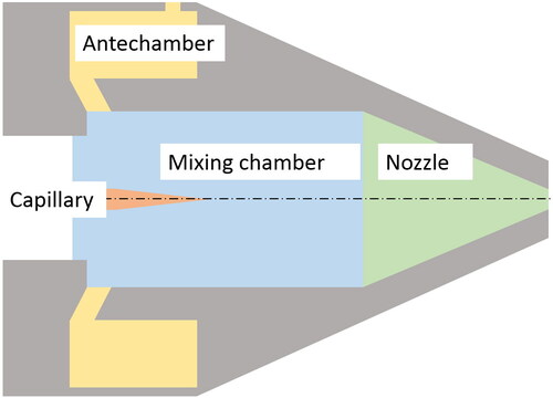
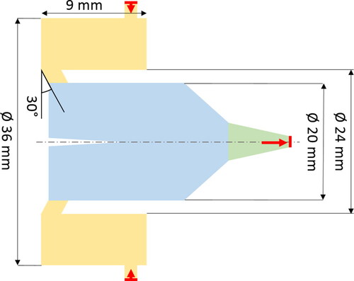
Modeling takes place on a workstation equipped with AMD Ryzen Threadripper 3970X processor with 32 cores, 64 threads @ 3,7GHz, 128 GB RAM, and a Nvidia Titan RTX graphics processor with 24GB. Figure 1 shows a schematic of the print head. The capillary, in which atomizing of the ink takes place, is excited by a rotationally symmetric piezo actuator and has a nominal diameter of 1.5 mm and a drawn tip of approx. 60 μm inner diameter. The tip of the capillary protrudes into the rotationally symmetric mixing chamber. The sheath gas used for aerodynamic focusing of the atomized ink flows into the mixing chamber through four inlets evenly distributed around the circumference. In order to achieve a homogeneous coaxial flow of the sheath gas around the capillary, the velocity profile of the sheath gas is homogenized in an antechamber. The outlet nozzle generating the aerosol jet has in a first version an orifice diameter of 1 mm, to enable fabrication by standard mechanical manufacturing processes. The atomized ink is modeled as distilled water in a discrete phase model with the sheath gas Argon as the continuous phase. Since the droplets in the print head only occupy a small volume fraction (<10% of the total volume), particle-particle interactions of the droplets is neglected. However, the momentum transfer of the aerosol to the sheath gas is not negligible for large aerosol mass flows, hence a coupling of the discrete phase with the continuous phase is implemented.

Figure 1. Schematic of the print head including capillary, antechamber, mixing chamber, and nozzle.

In preliminary studies (Benitez 2016), worst-case estimates of the aerosol properties at the outlet of the capillary were determined (see Table 1). We use this parameter-set as input variables for the simulations, with the aim of developing a robust geometry ensuring error-free operation not only under worst-case conditions, but also under a wide range of aerosol parameters. Starting with the aerosol properties as shown in Table 1 the operating point of the print head is determined. At this operating point, the relationship between nozzle angle and position of the focal point is analyzed in a subsequent simulation. Based on these results, the geometry of the antechamber is optimized with respect to a homogeneous distribution of the sheath gas. Based on the individual investigations, an overall model is created and the entire print head is simulated.

Table 1. Simulation parameters of the aerosol at the outlet of the capillary.

Parameter	Value
max. exit angle [°]	25
max. diameter of droplets [µm]	20
max. exit velocity [m/s]	10
max. aerosol mass flow [kg/s]	1.21 10-5

2.2.1. Determination of the operating point

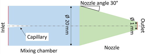
Criteria for error-free operation, and hence for the determination of the operating point of the print head, are on the one hand the stationary behavior of the droplets without wetting of the inner wall of the nozzle and on the other hand a focusing of the aerosol jet in freespace over a length of several millimeters. To determine the operating point a reduced model only consisting of the capillary, the mixing chamber, and the nozzle is used with a fixed nozzle angle of 30° (see Figure 2). The mesh consists of 250,968 elements with 63,635 nodes and a minimum edge length of 60 µm. Generation of the prism layers is conducted with a transition rate of 0.272 and a growth rate of 1.2. As boundary conditions, a pressure outlet at the nozzle orifice and a homogeneous mass flow inlet at the mixing chamber are selected. Influences of the antechamber and the free jet are not taken into account. In the simulations, the mass flows of the sheath gas and the aerosol are varied: A reduction of the mass flow of the sheath gas leads to a proportional decrease of the Reynolds number at the nozzle outlet, while a variation of the mass flow of the aerosol has no influence on the Reynolds number. Decreasing the mass flow will reduce the momentum transfer of the aerosol to the sheath gas.

Figure 2. Simulation model for determining the operating point.

The simulations resulted in convergent stationary solutions with residuals well below 10⁻⁴. The results are shown in Figure 3 in double logarithmic representation. Crosses represent the parameter combination of the simulations: upright crosses indicate parameter combinations with successful function, i.e., without wall contact, while tilted crosses indicate parameter combinations where the aerosol comes into contact with the wall and hence no proper operation is possible. The dashed straight line indicates the limit range of functioning operating points. The diagram enables determination of a maximum aerosol mass flow at a defined mass flow of the sheath gas (corresponding to the Reynolds number).

Figure 3. Mass flow of the sheath gas (Argon) over aerosol mass flow in double logarithmic representation. Upright crosses: Parameter combinations with successful function (no wall contact), tilted crosses: No functioning operation is possible (wall contact of the aerosol). The dashed straight line gives the limit range of functioning operating points. Circle: Operating point chosen for further simulations.

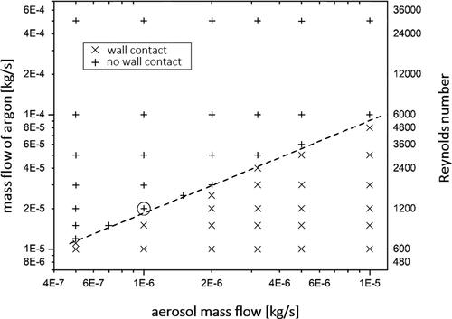
Provided the mass flow of the aerosol does not exceed 10% of the mass flow of the entire jet, the map of Figure 3 can serve as fundament to set the operating point. Knowing the relationship between sheath gas mass flow and aerosol mass flow, we can modify our worst-case assumption of the aerosol mass flow (see Table 1). Since, already from Reynolds numbers of Re ≈ 1500 at the nozzle outlet, turbulence occurs (Fernández de la Mora and Riesco-Chueca 1988), in further simulations we set our operating point at a Reynolds number of Re = 1200, which corresponds to a mass flow of the sheath gas of 2 × 10⁻⁵ kg/s (circle in Figure 3).

2.2.2. Focusing of the aerosol jet

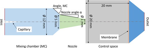
Based on the operating point determined in section 2.2.1, focusing of the aerosol can be further investigated. The model also allows simulation of the free jet behavior after the nozzle exit (see Figure 4). The corresponding control volume has no-shear boundary conditions on the sides (i.e., no shear stress can be transmitted) and is limited by a membrane. Behind this membrane, a conical area prevents negative mass flows in the outlet and thus stabilizes the simulation. The membrane is only permeable for the sheath gas, hence the aerosol cannot enter the conical outlet. This further stabilizes and accelerates the simulation, as there is no calculation of droplet trajectories in the outlet. The mesh consists of 1,706,866 elements with 311,231 nodes and a minimum edge length of 60 µm. Generation of the prism layers is conducted with a growth rate of 1.2. The realizable nozzle angle α depends largely on the selected manufacturing process. Since a nozzle with a larger opening angle is generally easier to manufacture than the aerodynamically advantageous long, flat nozzle, the angle is subdivided into a chamber angle and the nozzle angle α. The chamber angle is fixed at 45°. The antechamber is neglected in the simulation, the sheath gas flows homogeneously into the mixing chamber.

Figure 4. Simulation model for determining the focus point.

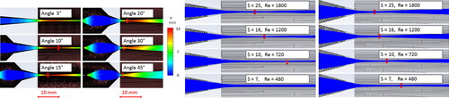
All simulations result in residuals of ≤1 × 10⁻⁴, so that convergence of the solutions is ensured. Figure 5, left shows the results of the variation of the nozzle angle on the position of the focal point at the operating point determined above. The simulation results show well the relationship between nozzle angle and focal point: The greater the nozzle angle, the shorter the distance of the focal point to the nozzle orifice. Printing on non-planar substrates requires a collimation of the droplets over several millimeters. This is achieved at angles of 5°, 10°, and 15°, as the focal points are more than 5 mm from the nozzle (see Figure 5). The calculated focus points depend on the nozzle angle α as well as on the Stokes number S (Kümmel 2007): If a critical Stokes number is undershot, there is no focusing outside the nozzle and the particle paths diverge after leaving the nozzle. In order to determine at which nozzle angle and which Reynolds numbers the critical Stokes number is undershot, simulations are carried out with varying Stokes numbers. Figure 5, right shows the results of these calculations for the nozzle opening angles 10° (left column) and 15° (right column). With a nozzle angle of 10°, the critical Stokes number is undercut at Re ≈ 500 (Figure 5, right, left column, third row). In order to be able to operate the print head also at Re ≈ 500, a nozzle angle of 15° is defined and used for further simulations and the final design of the print head.

Figure 5. Left: Trajectories of the droplets in dependence of the nozzle angle. Red marked is the respective position of the focal point. Right: Variation of the Stokes number for two nozzle angles (10°, 15°).

2.2.3. Design of the antechamber

So far, a homogenous flow of the sheath gas into the mixing chamber was assumed, which is necessary to obtain a uniform, rotationally symmetric aerosol jet. To homogenize the sheath gas flow commonly an antechamber is used. Due to manufacturability, we model an antechamber with four inlets, equidistantly distributed around the circumference and with a diameter of 1 mm each. The velocity distributions in the mixing chamber are used to analyze the flows: A homogeneous flow is achieved when a rotationally symmetric velocity profile is present in the mixing chamber. The initial model of the simulations contains a single, large antechamber, which fills the entire space (maximum diameter 36 mm, maximum length 9 mm, see Figure 6), predefined for the antechamber.

Figure 6. Initial model for the optimization of the antechamber. Red arrows: in- and outlets.

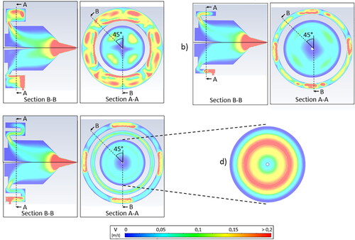
In the optimization step, different geometries of the antechamber are investigated. Since the aerosol is not important for the homogenization of the sheath gas flow, modeling of the aerosol was omitted in the following simulations. The results of the geometrical variations during optimization are shown in Figure 7 for three different configurations: Figure 7a) shows the velocity distribution of the initial model, subsequently the diameter was varied (see Figure 7b), followed by the variation of the length of the antechambers, leading to a folded structure (see Figure 7c). Within the antechamber, clear inhomogeneities in the velocity distribution can be observed in all variants. Tangentially oriented vortices (clearly visible in Figure 7a) formed by the radial inlet, lead to mixing in the circumferential direction. The deflection in the channel between the antechamber and the mixing chamber causes additional mixing, so that the velocity profiles within the mixing chamber are much more homogeneous than in the antechamber. A slim antechamber (see Figure 7b) improves the homogeneity compared to a wide antechamber (see Figure 7a). Assuming a laminar flow, this is due to the stronger velocity gradients in the radial direction, so that faster mixing occurs in the circumferential direction. By comparison, the best homogenization can be achieved by a double deflection (see Figure 7c). Within the mixing chamber no inhomogeneities in the velocity profile can be detected (see Figure 7d). The reason for this is the doubled distance in the antechamber as well as the additional sharp redirection of the flow, which both increases the pressure drop resulting in a more homogeneous flow field. Hence, a folded antechamber is chosen as the design for the print head.

Figure 7. (a) to (c) Velocity distributions in the antechamber outer rings and the mixing chamber inner disk for three different geometries of the antechamber. The dashed lines specify the direction of the respective profile. (d) Scaled velocity distribution in the mixing chamber only (design case Figure 7c).

2.2.4. Modeling of the entire print head

Based on the optimized geometries of the individual subsystems and the determined operating point, the entire print head is simulated in printing mode. For this purpose, all subsystems from antechamber to substrate are considered. The substrate is modeled as a wall, which stops the discrete phase (trap condition). The mesh consists of 4,107,235 elements with 1,097,103 nodes and a minimum edge length of 60 µm. Generation of the prism layers is conducted with a transition rate of 0.272 and a growth rate of 1.2.

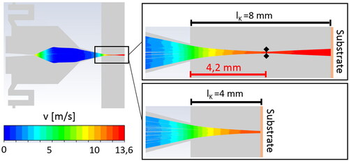
Result of the stationary simulation is a focused aerosol jet with a diameter of approx. 0.8 mm when leaving the nozzle and approx. 0.15 mm at the focus point. The focus point is at a distance of 4.2 mm from the nozzle (see Figure 8). There is no wall contact and the flows are rotationally symmetrical. Thus, all objectives are fulfilled. The distance between the print head and the substrate has no influence on the paths of the droplets (see Figure 8). It influences neither the position of the focal point nor the velocities of the droplets.

Figure 8. Simulation of the velocity progression in the droplet tracks. Left: of the entire print head; right: zoomed section with substrate distance of 8 mm (top) and substrate distance adjusted to the appropriate printing distance.

This proves that stationary solutions are formed everywhere in the free jet. Even at higher Reynolds numbers up to Re = 2400 there is no unsteady behavior of the sheath gas or the droplets. Without a stationary solution, reproducible results in the printing process would not be possible. Our results prove that the presented concept of the print head is suitable for functional printing and can be operated successfully with the optimized geometry and the specified operating point.

3. Experimental characterization of the laboratory setup

A first simple analysis of the jet forming process with a print head fabricated with the shape derived from the simulations above is carried out using optical methods. For this purpose, the refraction of light at the aerosol jet is used so that the individual droplets become visible under illumination. The body of a syringe, attached to a stand, serves as a reservoir. The hydrostatic pressure of the liquid column in the capillary can be varied via the vertical position Δz of the reservoir. As sheath gas, argon is fed from a pressure cylinder via a pressure regulator and a manual throttle into the mixing chamber of the print head. The entire test setup is shown schematically in Figure 9.

Figure 9. Schematic of the experimental setup.

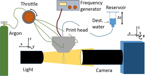
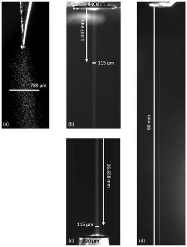
The droplets are examined with a Keyence VH-Z20R/Z20T light microscope (Z00 zoom objective; x30 and 0.29 ms exposure time for Figure 10a), x5 and 20 ms exposure time for Figure 10b, and x50 and 20 ms exposure time for Figures 10c and d) under a lateral illumination of 45° to the optical axis of the microscope. A Tapfer 5004LTF with a 20 W Cree LED with a luminous flux of 1440 lm is used as light source for our laboratory setup. Figure 10 shows images of the aerosol generated at the capillary tip (Figure 10a), focused by means of the sheath gas at the nozzle orifice (Figure 10b), onto a target tip at a distance of 27 mm (Figure 10c), and over a free space distance of 60 mm to obtain a qualitative impression of the jet propagation (Figure 10d). Already at a distance of 1.447 mm below the nozzle orifice, the focused beam width is 115 µm (see Figure 10b). This beam width remains stable over a collimation length of more than 25 mm (see Figure 10c) with a deviation of less than 1 µm. The nozzle diameter and the diameter of the target tip serve to estimate the width of the jet, respectively. Comparing the beam width of the focused and the unfocused aerosol jet shows focusing by a factor of approx. 7. Thus, it is proven that an aerodynamic focusing is achieved by means of the nozzle and the coaxial sheath gas flow. The achievable resolution of the printing process and thus of the printed patterns is not determined by the diameter of the aerosol jet alone. Other factors play also a role, such as the properties of the substrate surface, the interaction between the substrate surface and the aerosol jet, which in turn depends strongly on the ink properties and composition.

Figure 10. Unfocused aerosol jet at the capillary (a), the jet focused with the aid of the sheath gas at the nozzle orifice (b), on a target tip at a distance of 27 mm (c), and the collimated jet over a distance of 60 mm (d).

By varying the two parameters sheath gas mass flow and excitation amplitude of the actuator the aerosol mass flow can be controlled. At the same time, both parameters influence the amount of focusing. They are therefore important process parameters for functional printing. Together with the printing speed and the distance of the print head to the substrate, these parameters allow the control of line width and line thickness. The ink pressure in the capillary is a further parameter, which is important for the optimization of the printing process.

The experiments show aerodynamic focusing of the droplets inside the print head and stable aerosol jets could be observed over periods of 60 min and longer. A stable on-off behavior of the jet is also observed, proving the potential application of the new print head for on-demand-operation.

4. Discussion

This article introduces a new concept of an aerosol jet-on-demand print head for functional printing. Fluid dynamic simulations are used to find a stable operating point as well as to optimize the geometrical design. Based on the design a first test specimen was fabricated. Both in the fluid dynamic simulations as well as in the experiments distilled water was used instead of functional ink. Since the aerodynamic focusing is not dependent on the dynamic viscosity of the ink or the particle content in the ink, an aerodynamic focusing of all fluids that can be atomized in the capillary is possible. If, due to density or diameter, the droplets of functional inks have a different momentum than the droplets of distilled water, the sheath gas mass flow can be adjusted so that a focusing of the aerosol jet is achieved. The focusability of the aerosol and the associated parameters are decisive variables for controlling the printing process. The focus point of the aerosol should be on the surface of the substrate during printing and should be as sharp as possible to achieve a minimum line width. Two central conditions must be met for the reliable functioning of the aerosol jet-on-demand print head:

1. Generation of a stable, focused aerosol beam,

2. No wetting of the inner wall of the nozzle with aerosol.

Both conditions could be validated in first experiments. The behavior of the droplets after leaving the nozzle shows great similarities to the simulations: The droplets move on almost parallel paths. This results in a focused aerosol jet with a diameter of 115 µm over a length of several millimeters. At the stationary operating point no wetting of the nozzle walls happens.

The experiments have succeeded in producing a permanently stable aerosol jet. A stable on-off behavior of the jet was also observed, illustrating the potential of the new print head for on-demand-operation. In future investigations, an experimental set-up will be built that allows all relevant flow and pressure parameters to be controlled and the aerosol jets to be characterized more precisely. Further measurement capabilities will also be added to the setup in order to be able to measure droplet sizes, droplet distribution and droplet velocities, amongst others. The metrological characterization as well as the measurement results will be coupled with the simulation models to generate a digital twin for aerosol print head development.

Appendix: Mathematical conventions

The mathematical equations for fluid flow and the discrete phase model used in this article are taken out of the Fluent theory guide of Ansys. There, the operator $\nabla ,$ referred to as grad, nabla or del represents the partial derivative of a quantity with respect to all directions in the chosen coordinate system. In Cartesian coordinates, $\nabla$ is defined to be 15 $$\frac{\partial }{\partial x}\overrightarrow{i}+\frac{\partial }{\partial y}\overrightarrow{j}+\frac{\partial }{\partial z}\overrightarrow{k} .$$15

The gradient of a scalar quantity is the vector whose components are the partial derivatives, for example the gradient of the pressure is 16 $$\nabla p=\frac{\partial p}{\partial x}\overrightarrow{i}+\frac{\partial p}{\partial y}\overrightarrow{j}+\frac{\partial p}{\partial z}\overrightarrow{k} .$$16

The gradient of a vector quantity is a second-order tensor. In a Cartesian coordinate system it can be written like this: 17 $$\nabla \left(\stackrel{\rightharpoonup }{v}\right)=\left(\frac{\partial }{\partial x}\overrightarrow{i}+\frac{\partial }{\partial y}\overrightarrow{j}+\frac{\partial }{\partial z}\overrightarrow{k}\right)\left(v_x\overrightarrow{i}+v_y\overrightarrow{j}+v_z\overrightarrow{k}\right) .$$17

The divergence of a vector quantity, which is the inner product between $\nabla$ and the vector is for example 18 $$\nabla ·\stackrel{\rightharpoonup }{v}= \frac{\partial v_x}{\partial x}+\frac{\partial v_y}{\partial y}+\frac{\partial v_z}{\partial z} .$$18

The Laplacian operator ${\nabla }^2$ or $\nabla ·\nabla ,$ for example for the temperature $T,$ has the following meaning: 19 $${\nabla }^{2}T= \frac{{\partial }^{2}T}{\partial x^2}+\frac{{\partial }^{2}T}{\partial y^2}+\frac{{\partial }^{2}T}{\partial z^2} .$$19

References

- Ansys. 2021. Ansys Fluent user’s guide: Release 2021 R2. Canonsburg, PA: ANSYS, Inc.
- Benitez, J. L. 2016. Fluiddynamische Simulation hinsichtlich der Fokussierung eines Aerosolstroms [Fluid dynamic simulation with regard to the focussing of an aerosol flow]. Karlsruhe, Germany: Karlsruhe Institute of Technology (KIT), Institute for Automation and Applied Informatics.
- Chang, J. S., A. F. Facchetti, and R. Reuss. 2017. A circuits and systems perspective of organic/printed electronics: Review, challenges, and contemporary and emerging design approaches. IEEE J. Emerg. Sel. Topics Circuits Syst. 7 (1):1–21. doi:10.1109/JETCAS.2017.2673863.
- Choi, H. W., T. Zhou, M. Singh, and G. E. Jabbour. 2015. Recent developments and directions in printed nanomaterials. Nanoscale 7 (8):3338–55. doi:10.1039/C4NR03915G.
- Cui, Z. 2016. Printed electronics: Materials, technologies and applications. Singapore: John Wiley & Sons.
- Das, R., and X. He. 2021. IDTechEx: Printed, organic and flexible electronics 2020–2030: Forecasts, technologies, markets. Accessed July 1, 2021. https://www.idtechex.com/en/research-report/flexible-gedruckte-und-organische-elektronik-2020-2030-prognosen-technologien-m-rkte/687.
- Derby, B. 2010. Inkjet printing of functional and structural materials: Fluid property requirements, feature stability, and resolution. Annu. Rev. Mater. Res. 40 (1):395–414. doi:10.1146/annurev-matsci-070909-104502.
- Duineveld, P. 2003. The stability of ink-jet printed lines of liquid with zero receding contact angle on a homogeneous substrate. J. Fluid Mech. 477:175–200. doi:10.1017/S0022112002003117.
- Essien, M. 2016. Apparatuses and methods for stable aerosol deposition using an aerodynamic lens system. United States Patent US 2016/0193627 A1.
- Fernández de la Mora, J., and P. Riesco-Chueca. 1988. Aerodynamic focusing of particles in carrier gas. J. Fluid Mech. 195 (1):1–21. doi:10.1017/S0022112088002307.
- Ganz, S., H. M. Sauer, S. Weißenseel, J. Zembron, R. Tone, E. Dörsam, M. Schaefer, and M. Schulz-Ruthenberg. 2016. Printing and processing techniques. In Organic and printed electronics: Fundamentals and applications, eds. G. Nisato, D. Lupo, and S. Ganz, 48–116. Singapore: Pan Stanford Publishing.
- Gosman, A. D., and E. Loannides. 1983. Aspects of computer simulation of liquid-fuelled combustors. J. Energy 7 (6):482–90. doi:10.2514/3.62687.
- Gupta, A. A., A. Bolduc, S. G. Cloutier, and R. Izquierdo. 2016. Aerosol Jet Printing for printed electronics rapid prototyping. IEEE International Symposium on Circuits and Systems (ISCAS), Montreal, QC, 866–869. doi:10.1109/ISCAS.2016.7527378.
- Hedges, M., and A. B. Marin. 2012. 3D Aerosol Jet Printing—Adding electronics functionality to RP/RM. Direct Digital Manufacturing Conference, Berlin. Accessed February 24, 2020. https://optomec.com/wp-content/uploads/2014/04/Optomec_NEOTECH_DDMC_3D_Aerosol_Jet_Printing.pdf.
- Keicher, D. M., A. Cook, E. P. Baldonado, and M. Essien. 2018. Apparatus for pneumatic shuttering of an aerosol particle stream. United States Patent US 10,058,881.
- King, B. H. 2014. Miniature aerosoljet and aerosol jet array. United States Patent US 8,640,975 B2.
- Kümmel, W. 2007. Technische Strömungsmechanik [Technical fluid mechanics]. 3. Auflage. Wiesbaden: Teubner. doi:10.1007/978-3-8351-9126-6_7.
- Larson, B. J., S. D. Gillmor, and M. G. Lagally. 2004. Controlled deposition of picoliter amounts of fluid using an ultrasonically driven micropipette. Rev. Sci. Instrum. 75 (4):832–6. doi:10.1063/1.1688436.
- Liu, G., M. Hirtz, H. Fuchs, and Z. Zheng. 2019. Development of dip-pen nanolithography (DPN) and its derivatives. Nano. Micro. Small 15 (21):1900564. doi:10.1002/smll.201900564.
- Magdassi, S. 2010. The chemistry of inkjet inks. Singapore: World Scientific Publishing.
- Magdassi, S., and A. Kamyshny. 2017. Nanomaterials for 2D and 3D printing. Weinheim, Germany: Wiley-VCH.
- Menter, F. R. 1994. Two-equation eddy-viscosity turbulence models for engineering applications. AIAA J. 32 (8):1598–605. doi:10.2514/3.12149.
- Mette, A., P. L. Richter, M. Hörteis, and S. W. Glunz. 2007. Metal Aerosol Jet Printing for solar cell metallization. Prog. Photovolt: Res. Appl. 15 (7):621–7. doi:10.1002/pip.759.
- Neotech. 2021. 3D printed electronics applications realised by Neotech AMT. Accessed October 19, 2021. https://neotech-amt.com/applications.
- Reinhold, I. 2017. Inkjet printing of functional materials and post-processing. In Nanomaterials for 2D and 3D printing, eds. S. Magdassi, and A. Kamyshny, 27–49. Weinheim, Germany: Wiley-VCH.
- Salary, R., J. P. Lombardi, M. S. Tootooni, R. Donovan, P. K. Rao, P. Borgesen, and M. D. Poliks. 2017. Computational fluid dynamics modeling and online monitoring of Aerosol Jet Printing process. J. Manuf. Sci. Eng. 139 (2):021015. doi:10.1115/1.4034591.
- Shaker, G., M. Tentzeris, and S. Safavi-Naeini. 2010. Low-cost antennas for mm-Wave sensing applications using inkjet printing of silver nano-particles on liquid crystal polymers. IEEE Antennas and Propagation Society International Symposium, Toronto, ON, 1–4. doi:10.1109/APS.2010.5562281.
- Sieber, I., R. Thelen, and U. Gengenbach. 2020a. Assessment of high-resolution 3D printed optics for the use case of rotation optics. Opt. Express. 28 (9):13423–31. doi:10.1364/OE.391697.
- Sieber, I., R. Thelen, and U. Gengenbach. 2020b. Enhancement of high-resolution 3D inkjet-printing of optical freeform surfaces using digital twins. Micromachines 12 (1):35. doi:10.3390/mi12010035.
- SIJTechnology. 2021. Accessed December 13, 2021. https://sijtechnology.com/en/.
- Sirringhaus, H., and T. Shimoda. 2003. Inkjet printing of functional materials. MRS Bull. 28 (11):802–6. doi:10.1557/mrs2003.228.
- Sonoplot. 2021. Accessed December 13, 2021. https://www.sonoplot.com.
- Subramanian, V., J. B. Chang, A. de la Fuente Vornbrock, D. C. Huang, L. Jagannathan, F. Liao, B. Mattis, S. Molesa, D. R. Redinger, and D. Soltman. 2008. Printed electronics for low-cost electronic systems: Technology status and application development. ESSCIRC 2008—34th European Solid-State Circuits Conference, Edinburgh, 17–24. doi:10.1109/ESSCIRC.2008.4681785.
- Suganuma, K. 2014. Introduction to printed electronics. New York, NY: Springer.
- Ungerer, M. 2020. Neue Methodik zur Optimierung von Druckverfahren für die Herstellung funktionaler Mikrostrukturen und hybrider elektronischer Schaltungen [New methodology for optimising printing processes for the production of functional microstructures and hybrid electronic circuits]. Dissertation, Karlsruhe, Germany: Karlsruhe Institute of Technology (KIT).
- Ungerer, M., A. Hofmann, R. Scharnowell, U. Gengenbach, I. Sieber, and A. Wenka. 2018. Druckkopf und Druckverfahren [Print head and printing method]. Patent: DE 10 2018 103 049.5.
- Wang, M.-W., D.-C. Pang, Y.-E. Tseng, and C.-C. Tseng. 2014. The study of light guide plate fabricated by inkjet printing technique. J. Taiwan Inst. Chem. Eng. 45 (3):1049–55. doi:10.1016/j.jtice.2013.08.021.
- Wilcox, D. C. 2006. Turbulenc modelling for CFD. 3rd ed. La Canada, CA: DCW Industries, Inc.
- Wu, W. 2017. Inorganic nanomaterials for printed electronics: A review. Nanoscale 9 (22):7342–72. doi:10.1039/C7NR01604B.
- Yokota, T., K. Kuribara, T. Tokuhara, U. Zschieschang, H. Klauk, K. Takimiya, Y. Sadamitsu, M. Hamada, T. Sekitani, and T. Someya. 2013. Flexible low-voltage organic transistors with high thermal stability at 250 °C. Adv. Mater. 25 (27):3639–44. doi:10.1002/adma.201300941.