Densities of internally mixed organic-inorganic particles from mobility diameter measurements of aerodynamically classified aerosols

Abstract

Accurate knowledge of particle density is essential for many aspects of aerosol science. Yet, density is often characterized poorly and incompletely for internally mixed particles, particularly for dry particles, with previous studies focused primarily on deliquescent (aqueous) droplets. Instead, densities for dry internally mixed particles are often inferred from mass composition measurements in combination with predictive models assuming ideal mixing, with the accuracy of such models not estimated. We determined particle densities from mobility diameter measurements (using a Scanning Mobility Particle Sizer, SMPS) for dried particles classified by their aerodynamic size (using an Aerosol Aerodynamic Classifier, AAC) for a range of two-component organic-inorganic particles containing known proportions of organic and inorganic species. We examined all permutations of mixing between four different organic (water soluble nigrosin dye, citric acid, polyethylene glycol-400, and ascorbic acid) and three different inorganic (sodium chloride, ammonium sulfate, and sodium nitrate) species. The accuracy and precision in our measured particle densities were ∼5% and ∼1%, respectively, for nonvolatile particles. Substantial deviations in particle density from ideal mixing (up to 20%) were observed. We tested descriptions of the non-ideal mixing for our systems by representing the volume change of mixing using Redlich-Kister (RK) polynomials in terms of mass fraction or in terms of mole fraction, with both approaches performing similarly.

Graphical Abstract

EDITOR:

• Jason Olfert

1. Introduction

Particle density is a critical property for many aspects of aerosol science. It impacts particle aerodynamic properties and is thereby important in understanding the dynamics and lifetimes of particles in air streams. These aerodynamic considerations are key to understanding the behaviors of respirable aerosols and therefore are central to the development of aerosolized pharmaceuticals for drug delivery to the lungs (Edwards et al. 1997, 1998), as well as for modeling the contribution of expiratory droplets to airborne transmission and inhalation of pathogens (Walker et al. 2021). Moreover, understanding and modeling the optical properties of particles and how they interact with sunlight requires us to consider particle density. At a fundamental level, the density influences the intensive optical properties (refractive index) of a particle as specified through the Lorentz-Lorenz relation (Liu and Daum 2008). In atmospheric models of aerosol radiative transfer, density descriptions for particles of different aerosol types are needed to calculate mass extinction and absorption coefficients which, in combination with inventories of mass emission rates for different species, allow calculation of the optical depth for aerosol layers (Edwards and Slingo 1996). The densities of many common types of particles remain poorly constrained and represented, even for those with relatively simple chemical compositions, such as pure black carbon (soot) particulates (Olfert and Rogak 2019). Adding further complication to this problem, aerosol particles are commonly internally mixed and can be highly heterogeneous in chemical composition, structure, and phase (Riemer et al. 2019).

Studies have focused on the measurement of density for macroscale (bulk) samples using techniques such as X-ray crystallography (Robie et al. 1967; Johnston and Hutchison 1942) and helium densitometry (Pusz et al. 2010) for solids, the oscillating U-tube method for liquids and gases (Sequeira et al. 2019; Ashcroft et al., 1990), and a magnetic suspension balance (Kuramoto et al. 2004; Wagner and Kleinrahm 2004) for liquids. These techniques provide high precision measurements for single-component bulk samples as well as for mixtures. We refer to these measured densities as material densities. However, the effective density (ρ_e) of a particle can be very different from that of the material density of the substance comprising the particle. Leaving a strict definition of ρ_e to Sect. 2, these differences can arise from the non-spherical and/or aggregate structures that often occur during particle formation, with these morphological effects distributing the particle mass over a larger volume compared to a bulk material (Olfert and Rogak 2019; Pagels et al. 2009; Zelenyuk et al., 2006). Besides morphological impacts on effective density, particles often have compositions that are completely inaccessible to bulk samples. For example, aqueous droplets are able to exist in metastable supersaturated concentration states with respect to the solute, with solute molalities that can exceed the bulk solubility limit by up to several orders of magnitude (Bzdek et al. 2020; Cai et al. 2016). Therefore, it is of key importance to be able to characterize particle densities in addition to material densities. Progress in this area requires new approaches and techniques that enable determinations of densities for different particle compositions and mixing states.

Predicting the densities of chemically complex, internally mixed particles relies on the application of suitable mixing rules. It is common for densities to be calculated using aerosol composition measurements in combination with mixing rules, but these rules often have no physical basis and are chosen for their simplicity. Additionally, there is typically little or no discussion of their accuracy. Most often, studies assume ideal mixing of mixture components. For example, Taylor et al. (2020) use aerosol mass spectrometry data in combination with a volume-fraction weighting of assumed densities for inorganic and organic components of biomass burning aerosol coatings. McMurry et al. (2002) used an ideal mixing rule to calculate the densities of ambient aerosols, assuming that the particles were internally mixed and with fractional contributions from individual inorganic components. These ideal mixing approaches ignore the non-ideal interactions that can occur between individual mixture components that contribute a volume change of mixing. For example, recent work has indicated that crystalline structures of inorganic salts are not able to form upon mixing with organic species in some situations, with large changes in the mixture density occurring for some mixing compositions (Cotterell et al. 2020; Radney and Zangmeister, 2018). The lack of information on how effective density depends on chemical composition, and therefore the lack of assessment of the accuracy of density mixing models, exists because techniques and measurement approaches to directly measure the effective density of particles have only recently become available. With the advent of new and sensitive approaches for effective density measurements for aerosol particles, it is timely for studies to be conducted of effective density dependencies on chemical composition that enable assessments of predictive mixing models. This is of particular importance to atmospheric aerosols, in which a single particle may contain many chemical components of both organic and inorganic species (Murphy et al. 2006).

Particle densities determined from combined measurements of the particle mass, mobility, and/or aerodynamic size distributions have been reported in recent years, and we refer the reader to the article by Peng et al. (2021) who summarize and compare these approaches. In particular, size-resolved density characterizations are achieved with high precision when two of these particle size metrics are measured in tandem such that the distribution in one metric is recorded for particles classified by another metric (Peng et al. 2021). For example, it has become widely adopted to record the particle mass distribution (using an instrument such as the Centrifugal Particle Mass Analyzer) for particles that are first classified by their mobility, or vice versa from measurements of the mobility diameter distribution (using a Scanning Mobility Particle Sizer; SMPS) for particles first classified by their mass (Hu et al. 2021; Radney and Zangmeister 2018; Eggersdorfer et al. 2012; McMurry et al. 2002). Either of these approaches can be applied to the characterization of effective density for ambient aerosol particles, or for those generated in the laboratory, but they require particles to be charged using a neutralizer immediately prior to the initial classification stage. The subsequent classification of the charged particles by either a mass or mobility analyzer suffers from a poor transmission efficiency because of the small fraction of charged particles following neutralization, with a majority of particles possessing no charge, thus degrading the sensitivity of downstream characterizations of particle size metrics. A very recent innovation is the development of the Aerosol Aerodynamic Classifier (AAC), which classifies particles by their aerodynamic size (or, more strictly, their relaxation time) (Tavakoli et al. 2014; Tavakoli and Olfert, 2013). As an AAC does not require particles to undergo any prior charging, it yields much higher transmission efficiencies (up to ∼5 times higher than the other aforementioned analyzers) while also removing the multiple charging artifacts that can confound retrievals of aerosol microphysical properties (Johnson et al. 2018; Tavakoli et al. 2014; Tavakoli and Olfert 2013). In this work, an AAC was used to select particles within a narrow range of aerodynamic diameter, and the mobility diameter of these classified particles was measured using an SMPS. The relationship between aerodynamic and mobility size was then used to determine the effective density of the particles.

Only a limited number of studies have examined effective densities of mixed particles. Studies on particles levitated in an electrodynamic balance have allowed the determination of densities for aqueous droplets containing dissolved inorganic or organic solutes (Lienhard et al. 2012; Tang et al. 1997); however, these methods are unable to determine the densities of dry particles that do not resemble perfect spheres, precluding determinations of particle densities at low relative humidity (RH). Indeed, in situ observations of atmospheric particle properties (e.g., optical properties) are largely made on particles that have been dried below their efflorescence RH (e.g., Haywood et al. 2021; Redemann et al. 2021; Wu et al. 2021; Taylor et al. 2020; Davies et al. 2019; Pistone et al. 2019). Zelenyuk et al. (2006) used Single Particle Laser Ablation Time-of-flight mass spectrometry to sample mobility-selected particles, enabling direct measurements of particle densities for dry organic-inorganic particles for two different mixing ratios of succinic or lauric acid with ammonium sulfate. These measurements did not allow for any assessment of density mixing models for the limited range of mixture compositions considered. To our knowledge, no study has yet determined the densities under dry conditions of internally mixed organic-inorganic particles of atmospheric relevance over a comprehensive range of mixture compositions to enable assessments of density mixing models.

In this work, we use the AAC-SMPS approach to investigate particle densities for two-component organic-inorganic particles containing known proportions of an organic and an inorganic species, examining all permutations of mixing between four different organic (water soluble nigrosin dye, citric acid, polyethylene glycol-400, and ascorbic acid) and three different inorganic (sodium chloride, ammonium sulfate, and sodium nitrate) species. The systems of interest are chosen because of their relevance to atmospheric aerosols or aerosol science more broadly. We develop and test density mixing models for our solid mixtures and assess the discrepancies that arise in these predictions when using simplistic ideal mixing rules. The following section explicitly defines effective density and describes the theoretical basis underpinning its determination using the AAC-SMPS approach. We then describe our experimental methods and chemical systems of interest (Sect. 3). Next, we build on studies by other authors to assess the performance of the AAC-SMPS measurement approach in terms of its accuracy, sensitivity, and reproducibility (Sect. 4.1). We then report effective density measurements for different organic-inorganic mixtures and develop and evaluate non-ideal mixing models to describe our measured densities (Sect. 4.2).

2. Density retrievals from mobility diameter measurements for aerodynamically classified particles

The effective density of a particle is defined as the ratio of the particle mass (m) to the volume of a sphere with a diameter equal to the particle mobility diameter (d_m) (Tavakoli & Olfert 2014): (1) $${\rho }_{\mathrm{e}}=\frac{m}{\left(\pi /6\right)d_{\mathrm{m}}^3}$$(1) For spherical particles, d_m is equivalent to the particle geometric diameter. The effective density can be determined from measurements of d_m (using an SMPS) for particles first classified on their relaxation time $\tau$ (i.e., their characteristic time of approach to constant velocity when subjected to both centrifugal and drag forces) using an AAC (Tavakoli and Olfert 2013). The AAC consists of two cylinders rotating in the same direction at the same speed that exert centrifugal forces on particles in the radial direction as they are passed through the gap between the cylinders, while a sheath flow transports the particles in the axial direction. By controlling the rotational frequency of the cylinders and the sheath flow rate, only particles within a very narrow range of selected relaxation times are transmitted. This relaxation time is equal to the product of the particle mass ($m={\mathrm{\rho }}_{\mathrm{e}}\frac{\pi }{6}{d}_{\mathrm{m}}^3$) and mobility ($B=\frac{C_c\left(d_{\mathrm{m}}\right)}{3\pi \mu d_{\mathrm{m}}}$) (Tavakoli and Olfert 2014; Tavakoli et al. 2014; McMurry et al. 2002): (2) $$\tau =mB=\frac{{\rho }_e{d}_{\mathrm{m}}^2{C}_c\left(d_{\mathrm{m}}\right)}{18\mu }$$(2) with $\mu$ the dynamic viscosity of air and C_c the Cunningham slip correction factor (Allen and Raabe 1982). This relaxation time can be expressed in terms of its aerodynamic diameter (d_ae), which is defined as the diameter of a spherical particle with density ${\rho }_e$ = ${\rho }_0$ = 1 g cm⁻³ that has the same relaxation time and given implicitly by the equation (Tavakoli and Olfert 2014; Tavakoli et al. 2014): (3) $$\tau =\frac{{\rho }_0{d}_{ae}^2{C}_c\left(d_{\mathrm{ae}}\right)}{18\mu }$$(3) Combining Equations (2)(2) $$\tau =mB=\frac{{\rho }_e{d}_{\mathrm{m}}^2{C}_c\left(d_{\mathrm{m}}\right)}{18\mu }$$(2) and (3)(3) $$\tau =\frac{{\rho }_0{d}_{ae}^2{C}_c\left(d_{\mathrm{ae}}\right)}{18\mu }$$(3) yields an expression for the effective density in terms of the particle aerodynamic and mobility diameters: (4) $${\rho }_e={\rho }_0\frac{d_{\mathrm{ae}}^2{C}_c\left(d_{ae}\right)}{d_{\mathrm{m}}^2{C}_c\left(d_{\mathrm{m}}\right)}$$(4) The AAC can be used to classify aerosol particles with a desired d_ae from a polydisperse ensemble, while a downstream SMPS measures their mobility diameter distribution. The value of d_m corresponding to the AAC-selected d_ae is determined and the effective density is calculated using Equation (4)(4) $${\rho }_e={\rho }_0\frac{d_{\mathrm{ae}}^2{C}_c\left(d_{ae}\right)}{d_{\mathrm{m}}^2{C}_c\left(d_{\mathrm{m}}\right)}$$(4) under the assumption that the particles are spherical. For spherical particles without voids, this calculated density is equal to the density of the bulk material constituting the particle (i.e., ρ_e = ρ_bulk). For spherical aerosol particles with voids, the effective density is less than the material density (Tavakoli and Olfert 2014; DeCarlo et al. 2004; Brockmann and Rader 1990), and for particles that are non-spherical (either with or without voids), the effective density derived by the above approach may differ from the material density by an amount that depends on the particle size and shape (Tavakoli and Olfert 2014; McMurry et al. 2002; Hinds 1999). It is common to use the dynamic shape factor (χ) to quantify the impact of particle shape on the discrepancy between the measured effective density and the density of the material constituting the particle (ρ_m), with higher χ values reducing the measured effective density to below that for the material density (DeCarlo et al. 2004). The dynamic shape factor is equal to unity for spherical particles, but is almost always greater than one for non-spherical particles (DeCarlo et al. 2004).

An approach that can be used to examine the dependence of the effective density on the mobility diameter is to express the particle mass as a power law relation in terms of d_m: (5) $$m=A{d}_m^f$$(5) with A a constant and f denoted as the mass-mobility exponent. The quantity f is equal to 3 for particles that do not consist of agglomerate chains, while it is in the range 1.96-2.18 for ZrO₂ particles (Eggersdorfer et al. 2012), 2.48 for soot particles from non-premixed flames (Olfert and Rogak 2019), 2-3 for soot particles from premixed flames (Cross et al. 2010), and 2.26 ± 0.05 for black carbon particles produced during the flaming combustion of sub-Saharan African biomass fuels (Pokhrel et al. 2021). Combination of Equations (1)(1) $${\rho }_{\mathrm{e}}=\frac{m}{\left(\pi /6\right)d_{\mathrm{m}}^3}$$(1) and (5)(5) $$m=A{d}_m^f$$(5) yields: (6) $${\rho }_e=\frac{6A}{\pi }{d}_m^{f-3}$$(6) This equation captures the size-dependence of effective density. The value f = 3 indicates that the density is size-independent. Substitution of Equation (6)(6) $${\rho }_e=\frac{6A}{\pi }{d}_m^{f-3}$$(6) for ${\rho }_p$ into Equation (4)(4) $${\rho }_e={\rho }_0\frac{d_{\mathrm{ae}}^2{C}_c\left(d_{ae}\right)}{d_{\mathrm{m}}^2{C}_c\left(d_{\mathrm{m}}\right)}$$(4) yields the expression: (7) $$\frac{6A}{\pi }{d}_m^{f-1}{C}_c\left(d_m\right)={\rho }_0{d}_{ae}^2{C}_c\left(d_{ae}\right)$$(7) Therefore, from measurements of d_m for different values of AAC-selected d_ae, the parameters A and f that yield the best fit can be determined, thereby enabling the size-dependent density to be determined using Equation (6)(6) $${\rho }_e=\frac{6A}{\pi }{d}_m^{f-3}$$(6) . However, it is highly unlikely that the retrieved f will take the exact value f = 3 even when sampled particles are perfect spheres because of measurement uncertainties in d_m and d_ae. Even small (e.g., 1%) differences in f from the value 3 would imply a size-dependent density, thus making it challenging to define the effective density, as a density at a reference diameter would need to be chosen. Therefore, in this work, effective densities are calculated according to Equation (4)(4) $${\rho }_e={\rho }_0\frac{d_{\mathrm{ae}}^2{C}_c\left(d_{ae}\right)}{d_{\mathrm{m}}^2{C}_c\left(d_{\mathrm{m}}\right)}$$(4) , and data are analyzed simultaneously using the approach summarized by Equation (7) only as a ‘quality control’ method to ensure that the sampled particles have a retrieved f within an arbitrarily chosen threshold of ±5% of f = 3, and therefore that they can be considered to have size-independent effective densities.

3. Experimental methods

Our approach to measuring effective density is summarized in Figure 1. Briefly, we generated hydrated particles by nebulizing an aqueous solution with a controlled solute composition. The flow rate through the nebulizer (TSI Portable Test Aerosol Generator, Model 3073) was maintained at ∼1 L min⁻¹ by adjusting the pressure of the gas flow at the nozzle inlet of the nebulizer. The sample then passed into a ∼5 L glass vessel that served as a buffer to prevent under- or over-pressuring of the downstream measurement instruments. One outlet of this glass vessel was connected to a HEPA filter to facilitate this buffering, and a second outlet allowed the sample to be drawn through our measurement instrumentation. The RH of the sample was reduced to less than 10% (as recorded by the downstream SMPS, see below, which used an RH probe to characterize the humidity of the sheath flow) by drawing the sample through an aerosol diffusion dryer (Cambustion Ltd., Aerosol Diffusion Dryer) filled with indicating silica gel desiccant. The aerosol sample was then classified using an AAC (Cambustion Ltd.).

Figure 1. Schematic diagram summarizing our experimental approach to measurements of aerosol density. HEPA filter is a High Efficiency Particle Air filter, AAC is an Aerodynamic Aerosol Classifier, DMA is a Differential Mobility Analyzer, CPC is a Condensation Particle Counter, and SMPS is a Scanning Mobility Particle Sizer.

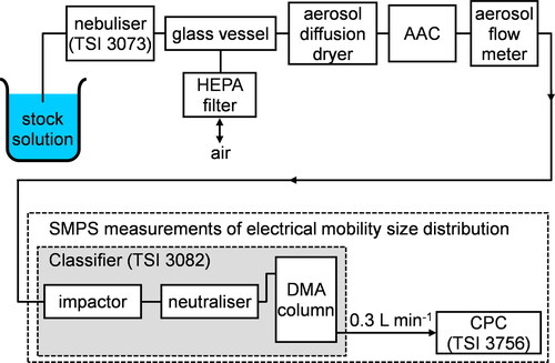
The sample transmitted by the AAC had a narrow distribution of aerodynamic diameters with a set-point value that was specified by the user. The resolution R_s of this transmitted distribution, defined as the ratio of the aerodynamic diameter set point to the full width at half maximum, was set to 20. Values of d_ae from 100 to 400 nm in 50 nm intervals were selected, with an additional value of 125 nm chosen for consistency with our early measurements. This d_ae range was chosen to allow subsequent accurate characterizations of particle mobility spectra using an SMPS, which were limited to an upper mobility diameter of <800 nm. For each value of d_ae, the mobility size distribution of the AAC-transmitted aerosol sample was characterized using an SMPS, which consisted of a TSI 3082 classifier utilizing a TSI 3088 Advanced Neutralizer, a TSI 3081 Differential Mobility Analyzer (DMA), and a TSI 3756 Condensation Particle Counter (CPC). The CPC operated at a flow rate of 0.3 L min⁻¹, which governed the flow rate through the diffusion dryer, AAC, and mobility classifier. The neutralizer imparted a bipolar charge distribution on the particles in the sample, and the particles were then selected by their mobility through an applied negative voltage to the center electrode of the DMA. This voltage was continuously scanned while the CPC recorded the number concentration of the mobility-classified particles. The sheath flow through the DMA column was set to 3 L min⁻¹ during these mobility distribution measurements, with a total scan time of 300 s over the mobility diameter range 50-600 nm. An inversion algorithm built into the manufacturer’s software (AIM, version 11.0) converted the raw measured size-dependent particle concentrations to a mobility diameter spectrum, with the standard corrections applied for multiple charging artifacts and diffusion losses. The delay time (t_d) was calculated automatically by the AIM software based on the length of tubing between the DMA and CPC (measured as 20 cm), and took a value of t_d = 1.72 s. All measurements were performed at ambient temperature and neither the temperature of the apparatus or the laboratory were regulated. The sample temperatures recorded by the SMPS during our measurement period were in the range ∼298 − 305 K. It was expected that the dependence of the measured densities on temperature would be very weak, as it is for most solids away from a phase transition.

The density retrieval approaches described in Sect. 2 require metrics for d_m corresponding to the nominal d_ae. We compared two different metrics for d_m (see Sect. 4.1). First, we used the modal mobility diameter corresponding to the largest amplitude in the recorded number size distribution (dN/dlog(d_m)), which we refer to as the mode-average d_m. Second, recognizing that the recorded mobility spectra had noise levels that could degrade the accuracy of the mode-average d_m and that the precision in this value is limited by the discrete number of measurement bins in an SMPS scan, we also used the derived modal diameter from the best fit of a bimodal lognormal distribution to the mobility diameter spectrum, which we refer to as d_m-fit.

Particles produced from solutions of two-component mixtures containing known mass fractions of an organic and an inorganic salt were studied. The mixture composition was controlled by dissolving known mass fractions of the chosen water-soluble organic (w_org) species and inorganic salt (w_inorg = 1 - w_org) in HPLC grade water, with a total solute mass of 1 g added to 80 ml of water. We were required to control the mass fractions, rather than mole fractions, of our solutes because the molecular weights for some of our solutes (specifically, nigrosin) were not known thereby precluding a mole fraction calculation. This aqueous solution was nebulized to generate our test particles using the procedure described above. It was assumed that the composition (i.e., organic-inorganic mass ratios) of the particles were the same as that of the solution. We note that the solubility limits of our chosen chemical species were all greater than ∼350 g L⁻¹ and therefore our aqueous solution concentrations (12.5 g L⁻¹) were well below these limits, removing any impact of solute solubility in our aqueous nebulizer solutions on the composition of our generated particles. Nominally, mixture compositions were varied systematically over the w_org range of 0.0 − 1.0 in 0.1 intervals. As measurements progressed, some additional compositions at intermediate w_org values were occasionally studied when the calculated density was found to be particularly sensitive to mixture composition. Repeat measurements were also performed for selected organic-inorganic mixtures at specific compositions. These repeats were mostly made in the early stages of our experimental studies when we were interested in the reproducibility of our derived densities. The value of ρ_e of a given organic-inorganic mixture composition was calculated using Equation (4)(4) $${\rho }_e={\rho }_0\frac{d_{\mathrm{ae}}^2{C}_c\left(d_{ae}\right)}{d_{\mathrm{m}}^2{C}_c\left(d_{\mathrm{m}}\right)}$$(4) from AAC-selected d_ae values and the measured mode-average d_m or fitted d_m-fit values. In addition, values of f and A were determined using Equation (7)(7) $$\frac{6A}{\pi }{d}_m^{f-1}{C}_c\left(d_m\right)={\rho }_0{d}_{ae}^2{C}_c\left(d_{ae}\right)$$(7) by minimizing the weighted least-squares residuals between $\left(6A/\pi \right)d_m^{f-1}{C}_c\left(d_m\right)$ and ${\rho }_0{d}_{ae}^2{C}_c\left(d_{ae}\right),$ with the retrieved f used only to check that the densities of the sampled particles could be considered as size-independent.

We determined the effective densities of two-component mixtures for all the permutations of mixing for four organic species with each of three inorganic salts. The inorganic salts used, ammonium sulfate (AS), sodium nitrate (SN), and sodium chloride (SC), were chosen because of their importance to atmospheric aerosol composition (Cotterell et al. 2017; Tang et al. 1997; Tang and Munkelwitz 1994). The organic species, water-soluble nigrosin dye (Nig, CAS code: 8005-03-6, batch number: BCBG2998V), citric acid (CA), polyethylene glycol 400 (PEG), and L-ascorbic acid (AA), were chosen based mostly on their importance to aerosol science, with Nig used widely to benchmark the performance of aerosol optical spectroscopy instruments (Cotterell et al. 2020; Davies et al. 2018; Langridge et al. 2016; Cappa et al. 2008), CA often used as a proxy for oxidized atmospheric aerosol (Choczynski et al. 2021; Marshall et al. 2016; Murray 2008), and PEG used to calibrate and compare instruments for aerosol volatility measurements (Bannan et al. 2019; Krieger et al. 2018; Mason et al. 2015). We decided to use AA after observing strong dependencies of ρ_e for mixed particles on nigrosin concentration. We postulated that this behavior could arise from strong polar interactions attributed to the aromatic groups reported to be present in nigrosin dye (Sedlacek and Lee 2007). AA contains a substituted furan group (an aromatic five-membered ring) and was an ideal system to further examine whether the presence of aromatic groups induced strong changes in effective density. Moreover, our choices of organic systems were constrained by the requirement that the sizes of the studied particles did not change appreciably between aerodynamic classification and subsequent measurement of mobility diameter distributions. If particles were to lose mass by evaporation of volatile components on the timescale of our measurements, negative biases in the measured d_m would arise that would result in overestimation of the effective density. Nig, CA, and AA are all solid powders at room temperature and therefore were assumed involatile, whereas PEG-400 is a liquid with a vapor pressure within the range 10⁻⁴–10⁻⁷Pa (Bannan et al. 2019). We examine below whether there is any impact of the small levels of mass loss expected for PEG on the accuracy of our retrieved effective densities.

4. Results and discussion

4.1. Accuracy and precision of density retrievals

Here, we explore measurements of densities for involatile solid particles for a range of pure (non-mixed) organic and inorganic species that do not adopt voided structures, and we compare our measured ρ_e against best measurements of corresponding material densities. We examine the impact of a range of factors on the accuracy of effective density retrievals, including the uncertainties in d_ae and d_m, the parameterization of the Cunningham slip correction, and the impact of particle volatility. There has previously been only a limited assessment of the precision and accuracy of effective density retrievals using the AAC-SMPS approach by Tavakoli and Olfert (2014), who reported values of 0.903 ± 0.090 g cm⁻³ for spherical droplets comprised of dioctyl sebacate, a liquid, which differed from the material density (0.913 ± 0.003 g cm⁻³) by only 1%.

4.1.1. Example measurement data and analysis considerations

Figure 2 shows examples of SMPS-measured mobility diameter distributions for AS particles classified by the AAC for various values of d_ae. Multiple peaks are observed in these distributions, which are particularly noticeable at higher values of d_ae; for example, three distinct peaks in d_m are observed when d_ae ≥ 300 nm. These peaks are attributed to particles that acquired multiple units of electric charge in the X-ray neutralizer. The charge distribution imparted to the aerosol sample passing through the neutralizer is Boltzmann-like, with charged particles with one unit of charge (q = 1) having a higher probability than higher levels of charge (q = 2, 3, etc.). Therefore, the peak with the largest amplitude for a given d_ae in Figure 2 occurs at the mobility diameter for the particles with q = 1 that are of interest for our density calculations.

Figure 2. Example mobility diameter distributions for dry, AAC-selected AS particles. The aerodynamic diameter d_ae selected by the AAC is indicated in each plot. The black circles are the measured concentrations at a given mobility diameter, while the red lines are the best fit of a bimodal lognormal size distribution to the measured data.

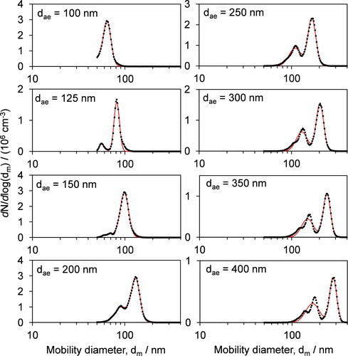
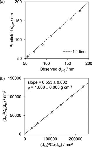
Importantly, the peaks attributed to multiple charging are observed even though the multiple charge correction was applied in the TSI SMPS software. To demonstrate that the observed peaks are indeed due to multiple charging, we calculated the modal diameter for the q = 2 particles (d_m,q=2) based on the observed modal mobility diameter for the q = 1 particles (d_m,q=1). As the mobility of a particle is directly proportional to the product of the charge on the particle and the Cunningham correction, and inversely proportional to the diameter (Stolzenburg and McMurry 2008), the mobility diameter d_q=2 of a particle with two elementary charges that has the same geometric diameter of a particle with mobility diameter d_q=1 with a single elementary charge satisfies the equation C_c(d_q=2)/d_q=2 = 2 C_c(d_q=1)/d_q=1. For the same mobility spectra shown in Figure 2, we compare the observed d_q=2 with our calculated values in Figure 3a. This comparison shows excellent agreement, demonstrating that the SMPS-measured peaks at lower diameters result from multiply charged particles.

Figure 3. (a) Comparison of calculated values of d_q=2 (as discussed in text) plotted against measured d_q=2 for the mobility spectra shown in Figure 2; the value for d_ae = 100 nm is not included because the mobility spectrum for this aerodynamic diameter does not extend to low enough mobility diameters to capture the d_q=2 mode. (b) Example plot of $d_{\mathrm{m}}^2{C}_c\left(d_{\mathrm{m}}\right)$ versus $d_{\mathrm{ae}}^2{C}_{\mathrm{c}}\left(d_{\mathrm{ae}}\right),$ including data points corresponding to the mobility size distributions in Figure 2. The linear regression of this distribution constrained through the origin enables the retrieval of the effective density of the sampled aerosols as the inverse of the slope of this line.

The presence of these multiple peaks in our mobility spectra indicates issues with the multiple charge correction algorithm implemented by TSI, possibly because the aerosol charging model applicable to X-ray neutralization may not be characterized accurately. The characterization of the charge distribution for X-ray neutralizers, first provided by Tigges et al. (2015b), has been shown to be dependent on operational conditions such as carrier gas, sample flow rate, RH, and the dielectric properties of the particles (Leppä et al. 2017; Tigges et al. 2015a). Indeed, our previous work has demonstrated issues with the charge model for X-ray neutralizers using another TSI classifier available in our laboratory (Cotterell et al. 2020). In this previous work, we reported that the measured optical properties for mobility-classified laboratory generated particles (as determined through high accuracy measurements using cavity ring-down and photoacoustic spectroscopy) could be reconciled with optical modeling predictions only through numerical optimization of the aerosol charge distribution that led to a different distribution required from that recommended by Tigges et al. The charging artifacts introduced by inaccuracies in the representation of X-ray neutralizer charging distributions are probably not commonly observed by many SMPS users who are looking at polydisperse samples, where the impacts of multiple-charge correction errors are not immediately obvious. Nevertheless, SMPS users should be aware of the potential for multiple-charge artifacts to introduce uncertainties and biases in their measurements even when applying the manufacturer’s multiple-charge correction.

The presence of multiple charge peaks was inconsequential to our effective density retrievals. Simply, we took the diameters for the q = 1 peaks in our mobility spectra. As described in Sect. 3, these mobility diameters were calculated from the mode-average diameters for the full spectrum (with the q = 1 peaks having the largest amplitude), but we also assess in Sect. 4.1.2 whether using a different determination of the peak diameters (taking the d_m-fit diameter of the q = 1 peaks as determined from the best fits of bimodal lognormal distributions) impacts the retrieved effective densities. As an example of the subsequent regression for the retrieval of effective density, Figure 3b shows the distribution in measured $d_{\mathrm{m}}^2{C}_c\left(d_{\mathrm{m}}\right)$ versus $d_{\mathrm{ae}}^2{C}_c\left(d_{\mathrm{ae}}\right)$ for the same measurement data set summarized in Figure 2. The linear regression of this distribution, constrained through the origin, has a slope that is the inverse of ρ_e, as shown by Equation (4). In this example, the effective density of pure AS particles was found to be 1.808 ± 0.008 g cm⁻³, with the uncertainty corresponding to the standard error in the slope. When repeat measurements were performed at some compositions, all measurement data for a given composition were aggregated and a single regression to all data was performed to retrieve the effective density. For pure AS particles, we performed one further repeat and the retrieved effective density from the combined regression was 1.804 ± 0.009 g cm⁻³, which agrees with the material density of 1.77 g cm⁻³ (Table 1) to within 2%.

Table 1. Comparison of ρ_e from our measurements on pure components with ρ_bulk values reported in the literature. The quoted errors in measured ρ_e represent the standard error in the density arising from our regression analysis.

Chemical species	Measured ρe/(g cm^-3)	Literature ρbulk/(g cm^-3)	$\frac{100\left({\rho }_{\mathrm{e}}-{\rho }_{\mathrm{bulk}}\right)}{{\rho }_{\mathrm{bulk}}}$
Ammonium sulfate (AS)	1.804 ± 0.009	1.765-1.772^1,2	+1.3 → +2.7
Sodium nitrate (SN)	2.187 ± 0.042	2.259-2.261^3-5	−1.3 → −5.1
Sodium chloride (SC)	2.061 ± 0.015	2.161-2.164^4,6,7	−3.9 → −5.5
Nigrosin dye (Nig)	1.632 ± 0.016	1.34-1.60^8-10	+1.0 → +23.0
Citric acid (CA)	1.688 ± 0.022	1.665^11	+0.1 → +2.7
Polyethylene glycol 400 (PEG)	1.240 ± 0.009	1.122-1.126^12-13	+9.3 → +11.3
Ascorbic acid (AA)	1.702 ± 0.020	1.694^14	−0.7 → +1.7

The quoted ranges in the percentage difference between our measured ρ_e and the literature density values arise from the standard error in our retrieved ρ_e and the range in reported literature density values. [1] Tutton (1906); [2] Johnston and Adams (1912); [3] Kracek (1931); [4] Robie et al. (1967); [5] Swanson et al. (1956); [6] Baxter and Wallace (1916); [7] Johnston and Hutchison (1942); [8] Moteki et al. (2010); [9] Radney and Zangmeister (2015); [10] Radney and Zangmeister (2018); [11] Bennett and Yuill (1935); [12] Rodríguez et al. (2012); [13] Sequeira et al. (2019); [14] Sonnergaard (2000).

4.1.2. Accuracy of density retrievals

One source of bias in our effective density retrievals is the determination of d_m (for the q = 1 particles) from measured mobility spectra. The systematic errors in measured mobility diameters directly connected to errors in the DMA sheath and excess air flow rates, geometric dimensions of the DMA, Cunningham slip correction, DMA voltage, and the measured sample pressure and temperature were assessed by Kinney et al. (1991). In their work, the authors assessed the systematic uncertainty in d_m to be ±3.0%. Propagating this level of systematic uncertainty in d_m through Equation (4)(4) $${\rho }_e={\rho }_0\frac{d_{\mathrm{ae}}^2{C}_c\left(d_{ae}\right)}{d_{\mathrm{m}}^2{C}_c\left(d_{\mathrm{m}}\right)}$$(4) indicates that the corresponding uncertainty in our derived ρ_e is 4.2%. In addition to these systematic errors, biases could arise in the mode-average diameter from noise in the measured aerosol number concentrations and the discretized distribution in mobility diameters. An alternative approach to determine d_m that mitigates against the impacts of CPC counting noise and allows determination of a continuous distribution in mobility, and therefore a precise determination of peak diameter, is to fit the mobility distributions to a multimodal lognormal distribution. We found that fitting our distributions to a bimodal lognormal distribution was sufficient to prevent biasing of the best fit distribution to the q = 1 mode, although inconsequential biases in the fit to q = 2 peaks are evident in Figure 2 when q = 3 peaks occur. We contrast the effective densities retrieved when using either the modal diameter calculated from a mode-average of the measured mobility spectra or the diameter d_m-fit for the q = 1 mode calculated from the best fit of a bimodal lognormal distribution. Figure S1 in the supplementary information (SI) compares effective densities determined using these two mobility diameter attribution methods and shows that, on average for all 147 particle values determined in this work, the density obtained when using the mode-average diameter is ∼0.8% lower than that obtained using the d_m-fit diameter from the bimodal lognormal fit. This level of bias in ρ_e is lower than the 4.2% standard error in ρ_e expected to be introduced from the aforementioned systematic errors involved in differential mobility analysis as assessed by Kinney et al. (1991). The main figures and tables presented in this article all report effective densities using mode-average mobility diameters, but corresponding figures using the d_m-fit mobility diameters are provided in the Supporting Information for completeness.

Any bias in the values of AAC-selected d_ae would constitute another source of systematic uncertainty in our retrieved effective densities. Traceable biases would result from uncertainties in the angular frequency of the AAC rotation, the internal dimensions of the AAC cylinders, the sheath flow rate, the description of the Cunningham slip factor, and the value for air viscosity (see Equations (1) and (19) in Tavakoli and Olfert (2013)). Immediately prior to this measurement campaign, our AAC was calibrated by the manufacturer, using a laser tachometer to ensure that the AAC rotational speed was within 1% of the specified value and a Gilibrator (Sensodyne) to ensure the sheath flow rate was within 2% of its specified flow rate. We assumed that the internal dimensions of the AAC classifier (length and radii) are known to within 0.5 mm of the values specified by the manufacturer, the Cunningham slip factor is known to within 2.5% (see below), and the viscosity of air is known to within ±1.3% given typical variations in the temperature of our laboratory during experiments. Assuming these uncertainties, we used standard propagation of error to estimate that the uncertainty in d_ae is ∼1.9%, which corresponds to a systematic error in effective density of ∼3.8%.

We investigated the magnitude of the uncertainty that arises from using different formulations of the Cunningham slip correction factor. We used the Cunningham slip correction described by Davies (1945) for spherical particles to determine the effective densities according to Equation (4)(4) $${\rho }_e={\rho }_0\frac{d_{\mathrm{ae}}^2{C}_c\left(d_{ae}\right)}{d_{\mathrm{m}}^2{C}_c\left(d_{\mathrm{m}}\right)}$$(4) . However, we recognize that there are many reported parameterizations of the Cunningham slip factor, and more recent parameterizations are available, such as those of Allen and Raabe (1985) and Kim et al. (2005), which have both been adopted widely by the aerosol science community. The Davies parameterization gives a Cunningham slip correction factor that is, on average, 2.5% larger than the other parameterizations over the diameter range 50 − 500 nm that is relevant to our work, and the retrieved effective densities using the Davies parametrization are approximately 0.3% less than the values calculated using the other parameterizations. Importantly, these differences are less than the precision in our regressed ρ_e.

Using the same approach as Johnson et al. (2020) in combination with our estimated uncertainty of 1.9% in d_ae and of up to 3.0% in d_m, we estimate the overall accuracy in ρ_e retrieved using Equation (4)(4) $${\rho }_e={\rho }_0\frac{d_{\mathrm{ae}}^2{C}_c\left(d_{ae}\right)}{d_{\mathrm{m}}^2{C}_c\left(d_{\mathrm{m}}\right)}$$(4) is 7.1%. This estimation approach ignores the small contribution from the Cunningham slip correction factor. As we show below, this estimate of 5.2% is near-identical to the better-than 5% agreement between our measured ρ_e for single component particles with literature values for material density.

The determination of effective densities in this work relies on a linear regression consistent with Equation (4)(4) $${\rho }_e={\rho }_0\frac{d_{\mathrm{ae}}^2{C}_c\left(d_{ae}\right)}{d_{\mathrm{m}}^2{C}_c\left(d_{\mathrm{m}}\right)}$$(4) , which is valid for particles with size-independent density. Significant bias could be introduced to our retrieved ρ_e if the effective densities are size-dependent. The f-factor analysis described in Sect. 2 was performed to assess whether there was any size dependence in our measured densities. Figure S2 in the SI shows that the f factors for all our aerosol mixtures and pure component systems were within ±5% of f = 3, the value that is expected when the density is size-independent. Therefore, the density is well approximated by the size-independent assumption of our linear regression approach. There is a possibility that the assumption of spherical shape is not valid for our particles and therefore the densities derived by our linear regression would need to be corrected for the particle dynamic shape factors. However, as we now show, our measured effective densities compare well with literature values for material densities, thus indicating that the shapes of our particles are well represented by the spherical assumption.

Table 1 summarizes our measurements of ρ_e for pure component aerosols comprised of the four organic and three inorganic species of interest, and value ranges reported in the literature for the material densities. Except for Nig and AA, we have been careful to include literature values for material densities that use crystallography methods for the solids or an oscillating U-tube for PEG-400 (a liquid), which represent the techniques-of-choice for accurate and precise measurements of crystalline solid and liquid material densities respectively. For the four crystalline structures, the material densities reported in Table 1 correspond to AS in the orthorhombic system, SC in the face center cubic crystal system, SN in the hexagonal crystal family with space group R3c (i.e., the most common crystal structure adopted by SN when crystallized from solution), and CA in the monoclinic system. We note that the latter substance is known to form hydrates during the crystallization from bulk solutions, but the material density reported here corresponds to the anhydrous form. Table 1 summarizes the range of percentage differences between our measured ρ_e and the material densities, considering the range of our measurement precision and the range of reported literature values. Our ρ_e values agree with the reported material densities to better than ∼5% for all substances, except for PEG-400 which is discussed further below. We highlight the large range in reported densities for nigrosin, for which there seems to be no consensus (Radney and Zangmeister 2015, 2018; Moteki et al. 2010). There are conflicting reports of the structure and chemical composition of nigrosin, and it is reported to be a mixture of polyanilines manufactured by heating nitrobenzene, aniline, and hydrochloric acid with a metal catalyst, before adding an orange dye to match a specific color index at a wavelength of 550 nm (Sedlacek and Lee 2007b; Bond et al. 1999). Indeed, Sedlacek and Lee (2007) suspected batch-to-batch and manufacturer variability in the properties of nigrosin dye.

Our measured ρ_e for PEG-400 particles is ∼10% greater than the material density (Table 1). While the other species we have discussed so far are solids at room temperature and can be considered as involatile species, PEG-400 is a liquid and is semi-volatile. The evaporative loss of PEG-400 between aerodynamic selection and characterization of particle mobility could bias our reported ρ_e in the observed direction by an amount that depends on the saturation vapor pressure of PEG-400 and the time over which evaporation occurs. The volatility of PEG-400 is not well characterized. Indeed, the composition of PEG-400 is not defined precisely, but instead consists of a mixture of polyethylene glycols with an average molecular weight in the range 380 − 420 g mol⁻¹. Mason et al. (2015) reported the evaporation rate for PEG-400 particles with a diameter of ∼3 µm as being 0.05 nm s⁻¹, corresponding to a vapor pressure of ∼2.9 × 10⁻⁴Pa. Logozzo and Preston (2021) reported a vapor pressure of ∼1 × 10⁻⁴Pa from measurements on single, optically trapped aerosol particles. Meanwhile, Krieger et al. (2018) performed limited assessments of the temperature-dependent saturation vapor pressures for octaethylene glycol (i.e., a polyethylene glycol with eight repeating units of the ethylene oxide and therefore a molecular weight of 370.4 g mol⁻¹), with measured values at 300 K ranging from 9.04 × 10⁻⁹Pa using an electrodynamic balance to 1.6 × 10⁻⁶Pa using Knudsen effusion mass spectrometry. Such a large range in estimates of single component vapor pressures, spanning several orders of magnitude, is common for semi-volatile organic compounds found commonly in the atmosphere, such as dicarboxylic acids (Bilde et al. 2015; Cai et al. 2015). Based on the volume of tubing between the AAC and classifier, the volume of our DMA column, and the aerosol sample flow rate of 0.3 L min⁻¹, we expect that the aerosol sample spends ∼100 s between AAC classification and exiting the mobility classifier (DMA column). Using this time delay with the Maxwell mass flux equation corrected for the transition regime (Cotterell et al. 2014; Krieger et al. 2012; Ray et al. 1989), and assuming a mean molecular weight of 400 g mol⁻¹ and a diffusion coefficient for PEG-400 in air equivalent to that for octaethylene glycol (3.68 × 10⁻⁶ m² s⁻¹, Krieger et al. (2018)), we can reconcile our measured ρ_e with the literature reported material density if the PEG-400 saturation vapor pressure is ∼1.3 × 10⁻⁴Pa. This value is reasonable and lies within the aforementioned range of available literature data. We note that that this analysis does not account for evaporation within the AAC instrument, which will bias high our estimated d_ae based on the user selected value. Nonetheless, this discussion serves to highlight that the difference between our measured ρ_e and material density for PEG-400 is likely caused by evaporation of the semi-volatile PEG between aerodynamic selection and characterization of the mobility diameter. Others should consider the limitations of particle characterizations using the AAC-SMPS approach when examining particles containing volatile components and care should be taken to ensure the impacts of volatility are accounted for or mitigated.

With the exception of PEG-400, the agreement between our measured ρ_e and reported material densities to better than ∼5% is confirmation that the aerodynamic behavior of our particles is well represented by models that assume a spherical shape and do not contain internal voids that would otherwise lower the effective density, and therefore the dynamic shape factors for these particles are well represented by the assumption χ = 1. The formation of spherical particles in our experiments is not unexpected, even for sodium chloride which has a face-center cubic crystal structure in the solid state. The spherical surface of an aqueous aerosol droplet can act as a template for crystal formation upon efflorescence (Hardy et al. 2021; Baldelli and Vehring 2016). Moreover, studies suggest that the drying of droplets with sub-micrometer diameters are more likely to form spherical particles than larger droplets. For example, Baldelli and Vehring (2016) report that aqueous SN droplets with sub-micrometer diameters dried to form spherical particles with high reproducibility, while larger particles adopted morphologies with higher surface roughness. The agreement between ρ_e and the material densities also indicate that the assumption that our particles are dry is reasonable. However, we cannot rule out entirely the possibility that all the generated particles are devoid of water; for example, macroscopic samples of CA crystallize to their monohydrate form when dried at temperatures below 34 °C (Lafontaine et al. 2013). It is also important to recognize that Table 1 provides the material densities for crystalline AS, SC, SN and CA; we are not able to confirm the presence or absence of amorphous domains in our generated particles, which may alter the measured effective densities.

4.1.3. Precision of density retrievals

The mean precision in the effective density, ${\mathrm{\sigma }}_{\rho },$ determined from the standard errors in the regression slopes for all 147 density retrievals performed in this work, including both pure and internally mixed particles, is 0.019 g cm⁻³ (or ±1.10%) when using the mode-average calculated d_m, and 0.016 g cm⁻³ (±0.94%) when using the d_m-fit from our bimodal lognormal fits. The higher precision is expected for the latter approach as it mitigates against the presence of noise in the measured mobility size distributions. The correlation between ${\mathrm{\sigma }}_{\rho }$ and ρ_e is weak, with Pearson correlation coefficients of 0.32 and 0.13 when using the mode-average d_m and d_m-fit mobility diameters, respectively. We highlight that these estimates of ${\mathrm{\sigma }}_{\rho }$ are better than that in the initial assessment of Tavakoli and Olfert (2014), who reported a measurement precision of 0.090 g cm⁻³ (or ±10.0%) from AAC-SMPS measurements of dioctyl sebacate droplets. Tavakoli et al. determined effective densities from measurements of d_m for single values of d_ae rather than applying a regression to a distribution in d_m with d_ae as is done in our work; indeed, if we repeat our density retrievals but use the same single measurement approach used by Tavakoli et al., the standard deviation in our measured ρ_e increases by approximately six-fold. Further differences may arise from differences in the stability and magnitude in particle number concentrations generated, which will impact the signal-to-noise ratio in measured mobility diameter spectra.

4.2. Density measurements for two-component organic-inorganic aerosol mixtures

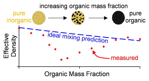
We now consider our measurements of ρ_e for internally mixed particles consisting of two-component organic-inorganic mixtures. Figure 4 shows our measured ρ_e distributions as functions of w_org. Importantly, Figure 4 shows that the trends in density with w_org are characterized sensitively, with the range in measured densities for a given mixture exceeding the measurement sensitivity. We also highlight that the bias of +10% in ρ_e for pure component PEG particles, as assessed in Sect. 4.1.2, is small compared to the density variation over the entire range of w_org. Almost all our mixtures demonstrate variations in ρ_e with w_org that deviate significantly from ideal mixing predictions. The mixtures involving nigrosin demonstrate particularly large deviations from what would be predicted from a simple ideal mixing rule, with ρ_e varying in a non-monotonic manner when Nig is mixed with any of our three inorganic salts.

Figure 4. Measurements of effective density as a function of organic mass fraction (w_org) for internally mixed, two-component particles containing an organic and an inorganic species. The open squares show all measurements of ρ_e, including repeat measurements at some mass fractions. The filled circles are the values that were included in fits of our non-ideal mixing rule (red lines) in the mass-fraction domain (keeping up to n = 2 in Equation (11)(11) $$V_{\mathrm{M}}=w_{\mathrm{org}}\left(1-w_{\mathrm{org}}\right)\sum _{k=0}^n{L}_{\mathrm{k}}{\left(2w_{\mathrm{org}}-1\right)}^k$$(11) ) and represent the best estimate of the effective density at a given w_org by including all data from repeat measurements in a single regression of $d_{\mathrm{ae}}^2{C}_{\mathrm{c}}\left(d_{\mathrm{ae}}\right)$ versus $d_{\mathrm{m}}^2{C}_{\mathrm{c}}\left(d_{\mathrm{m}}\right).$ The error bars indicate the standard error in the determined slope of $d_{\mathrm{ae}}^2{C}_{\mathrm{c}}\left(d_{\mathrm{ae}}\right)$ versus $d_{\mathrm{m}}^2{C}_{\mathrm{c}}\left(d_{\mathrm{m}}\right)$ distributions. The blue dashed line is the ideal mixing rule prediction (Equation (9)(9) $${\rho }_{\mathrm{ideal}}=\frac{1}{\frac{w_{\mathrm{org}}}{{\rho }_{\mathrm{org}}}+\frac{\left({1-w}_{\mathrm{org}}\right)}{{\rho }_{\mathrm{inorg}}}}$$(9) ). Note that the different rows of plots have differing vertical scale value ranges.

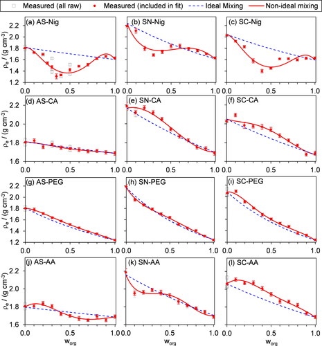
Although, in principle, the observed deviations in ρ_e from ideal mixing could arise from deviations in the dynamic shape factor from χ = 1 (see discussion in Sect. 2), there are several reasons why we do not expect such deviations to occur. First, Sect. 4.1.2 shown that the measured ρ_e for single component particles were in excellent agreement with best estimates of material densities available in the literature, indicating χ = 1, although we acknowledge that this assessment does not necessarily pertain to particles when internally mixed. Second, the ρ_e in Figure 4 show both positive and negative deviations from the expectation of ideal mixing; if the positive deviations were attributable to changes in particle shape, χ would have to be less than unity to reconcile the measured ρ_e with ideal mixing, yet χ is almost always greater than one for non-spherical particles (DeCarlo et al. 2004). The analysis below therefore assumes our sampled particles are spherical and that deviations in ρ_e from ideal mixing arises from the effects of non-ideal interactions between mixing species, but we acknowledge that the potential for impacts of particle shape cannot be ruled out completely. For mixtures of SN with either CA or AA, a further factor that could impact on measurements of ρ_e, and cause differences with respect to ideal mixing predictions, is the evaporative loss of nitrate (as HNO₃) upon particle drying (Wang and Laskin 2014). However, we are not concerned with this evaporative loss given the relative timescales of our measurements following particle drying (∼2 min) and those of the loss of nitrate in typical dry particles of SN internally with organic acids; Wang and Laskin (2014) showed that the characteristic timescale for ∼50% of the nitrate to be lost by evaporation, from SN particles internally mixed with a range of organic acids, to be ∼4 weeks. Moreover, as we shown in Sect. 4.1.2 for measurements on semi-volatile PEG-400 particles, the impacts of significant evaporation of particle mass between AAC selection and mobility characterization would manifest as a consistent positive bias in ρ_e from the ideal mixing prediction. Yet, this effect was only moderate for PEG-400. For mixtures of SN with either CA or AA, positive deviations in ρ_e from ideal mixing are observed for some mixture compositions with CA, but only negative deviations are observed for mixtures with AA. Therefore, the impacts of acidity on the evaporation of nitrate are negligible on the timescales of our measurements.

We now investigate the representation of our measured ρ_e for organic-inorganic mixtures by mixing rule models. In the following, we first derive an expression for the mixture density that considers only ideal mixing. Next, we modify the ideal mixing expression to include a correction that accounts for non-ideal interactions between the organic and inorganic species. We fit this model to our measured density distributions in the mass-fraction domain to assess the particle volume change on mixing and the deviations in the mixture densities from ideal mixing. We repeat these comparisons when fitting our non-ideal mixing model in the mole-fraction domain.

4.2.1. The ideal mixing rule for predicting the densities of mixtures

We consider the mixing of species with known mass fractions w_i. The ideal mixing rule for density assumes that the total volume of a mixture is the sum of the individual volumes and is given by: (8) $${\rho }_{\mathrm{ideal}}=\frac{m}{V}=\frac{m}{\sum _i\frac{m_i}{{\rho }_i}}=\frac{1}{\sum _i\frac{w_i}{{\rho }_i}}$$(8) in which m and V are the total mass and volume of the mixture, respectively, and m_i, ρ_i, and w_i are the mass, density, and mass fraction of component i, respectively. We have chosen to represent the ideal mixing rule in terms of mass fraction because we control (measure) the component mass fractions when we formulate our aqueous solutions for nebulization. For our two-component organic-inorganic mixtures with an organic mass fraction w_org and an inorganic salt mass fraction w_inorg = 1 – w_org: (9) $${\rho }_{\mathrm{ideal}}=\frac{1}{\frac{w_{\mathrm{org}}}{{\rho }_{\mathrm{org}}}+\frac{\left({1-w}_{\mathrm{org}}\right)}{{\rho }_{\mathrm{inorg}}}}$$(9) in which ${\rho }_{\mathrm{org}}$ and ${\rho }_{\mathrm{inorg}}$ are the pure component densities of the organic and inorganic species, respectively. These two pure component densities are varied using the same least squares fitting method described in Sect. 4.2.2, and the results of these fits are shown in Figure 4.

4.2.2. Non-ideal mixing in the mass-fraction domain

Equation 9 assumes ideal mixing in that the total mass is the sum of the individual masses and the total volume is the sum of the individual volumes of the components ($m_i/{\rho }_i$). Although the total mass is always conserved, most chemical systems exhibit non-ideal mixing in which the total volume is not. Therefore, we modify Equation (9)(9) $${\rho }_{\mathrm{ideal}}=\frac{1}{\frac{w_{\mathrm{org}}}{{\rho }_{\mathrm{org}}}+\frac{\left({1-w}_{\mathrm{org}}\right)}{{\rho }_{\mathrm{inorg}}}}$$(9) by adding a term that describes the change in the total volume of the system due to non-ideal mixing: (10) $${\rho }_{\mathrm{mix}}=\frac{1}{\frac{w_{\mathrm{org}}}{{\rho }_{\mathrm{org}}}+\frac{\left({1-w}_{\mathrm{org}}\right)}{{\rho }_{\mathrm{inorg}}}+V_M}$$(10) in which V_M is a mass-normalized volume change on mixing, which depends on w_org. The functional form of V_M must recognize that V_M = 0 in the limits w_org = 0 and w_org = 1; i.e., there is no volume change on mixing when the generated particles are composed of either the pure organic or inorganic species. Such a functional form can be represented by a polynomial expansion in which each factor contains the term w_org(1 − w_org). Redlich and Kister (1948) proposed a polynomial expansion that is commonly used to describe excess thermodynamic properties for mixtures (Zardini et al. 2010; Singh et al. 2009). We therefore use the Redlich-Kister polynomial expansion and write V_M as: (11) $$V_{\mathrm{M}}=w_{\mathrm{org}}\left(1-w_{\mathrm{org}}\right)\sum _{k=0}^n{L}_{\mathrm{k}}{\left(2w_{\mathrm{org}}-1\right)}^k$$(11) in which L_k is the Redlich-Kister (RK) coefficient for polynomial order k. The model described by Equations (10)(10) $${\rho }_{\mathrm{mix}}=\frac{1}{\frac{w_{\mathrm{org}}}{{\rho }_{\mathrm{org}}}+\frac{\left({1-w}_{\mathrm{org}}\right)}{{\rho }_{\mathrm{inorg}}}+V_M}$$(10) and (11)(11) $$V_{\mathrm{M}}=w_{\mathrm{org}}\left(1-w_{\mathrm{org}}\right)\sum _{k=0}^n{L}_{\mathrm{k}}{\left(2w_{\mathrm{org}}-1\right)}^k$$(11) for mixture density (${\rho }_{\mathrm{mix}}$) was fitted to our measured effective densities (${\rho }_{\mathrm{e}}$) by varying the parameters ${\rho }_{\mathrm{org}},$ ${\rho }_{\mathrm{inorg}},$ and the polynomial coefficients L_k such that the sums of the weighted least-squares residuals: (12) $$R=\sum _i\frac{{\left({\rho }_{i,\mathrm{e}}-{\rho }_{i,\mathrm{mix}}\right)}^2}{{\rho }_{i,\mathrm{e}}^2}$$(12) were minimized, with ${\rho }_{i,\mathrm{e}}$ and ${\rho }_{i,\mathrm{mix}}$ the measured and modeled densities, respectively, at an organic mass fraction w_org,i, and the summation is over all i measured effective density values. We experimented with different versions of this merit function, experimenting also with versions of Equation (12)(12) $$R=\sum _i\frac{{\left({\rho }_{i,\mathrm{e}}-{\rho }_{i,\mathrm{mix}}\right)}^2}{{\rho }_{i,\mathrm{e}}^2}$$(12) where no weighting for the measured density is included, or weighting instead for the uncertainty (standard error) in the measured ρ_e, but we found that the choice of merit function was of little consequence in reducing the fit residuals between our measured ρ_e and the best-fit non-ideal mixing model. To mitigate against biasing our fit to regions of w_org where repeat measurements of ρ_e were made (open squares in Figure 4), we fit our model to the ρ_e derived from the regression of all repeat data at a given w_org (filled circles in Figure 4). We truncated Equation (11)(11) $$V_{\mathrm{M}}=w_{\mathrm{org}}\left(1-w_{\mathrm{org}}\right)\sum _{k=0}^n{L}_{\mathrm{k}}{\left(2w_{\mathrm{org}}-1\right)}^k$$(11) at n = 2, beyond which there was little improvement in the model fit to measured ρ_e, as discussed below.

Figure 4 shows the best fits of Equations (10)(10) $${\rho }_{\mathrm{mix}}=\frac{1}{\frac{w_{\mathrm{org}}}{{\rho }_{\mathrm{org}}}+\frac{\left({1-w}_{\mathrm{org}}\right)}{{\rho }_{\mathrm{inorg}}}+V_M}$$(10) and (11)(11) $$V_{\mathrm{M}}=w_{\mathrm{org}}\left(1-w_{\mathrm{org}}\right)\sum _{k=0}^n{L}_{\mathrm{k}}{\left(2w_{\mathrm{org}}-1\right)}^k$$(11) to our measured ρ_e, with the best fit parameters for these curves summarized in Table 2. The corresponding best fit V_M distributions are shown in Figure 5, which are compared against measured V_M values determined from the difference between our measured ${\rho }_{\mathrm{e}}^{-1}$ and calculated ${\rho }_{\mathrm{ideal}}^{-1}.$ Figure 5 clearly demonstrates the convergence of our best-fit V_M to our measured values as Equation (11)(11) $$V_{\mathrm{M}}=w_{\mathrm{org}}\left(1-w_{\mathrm{org}}\right)\sum _{k=0}^n{L}_{\mathrm{k}}{\left(2w_{\mathrm{org}}-1\right)}^k$$(11) is truncated at ever higher values of n. We find that truncating Equation (11)(11) $$V_{\mathrm{M}}=w_{\mathrm{org}}\left(1-w_{\mathrm{org}}\right)\sum _{k=0}^n{L}_{\mathrm{k}}{\left(2w_{\mathrm{org}}-1\right)}^k$$(11) at n = 2 is optimal for capturing the measured trends in V_M; comparison when including higher order RK polynomial terms (see Figures S5 and S6 in the SI) leads to trends that are unlikely to reflect true physical changes in V_M and for which the improvement in the least square residual (Equation (12)(12) $$R=\sum _i\frac{{\left({\rho }_{i,\mathrm{e}}-{\rho }_{i,\mathrm{mix}}\right)}^2}{{\rho }_{i,\mathrm{e}}^2}$$(12) ) is only marginal. V_M takes large values for some mixture compositions that involve Nig, with values as large as 0.15 cm³ g⁻¹ for mixtures of AS or SC with Nig. Meanwhile, for mixtures with other organics, values of V_M are substantially less. Indeed, V_M is negligible for AS-CA mixtures, with deviations less than 0.01 cm³ g⁻¹ that are within the noise of measured V_M; thus, mixed AS-CA particles can be considered as ideal mixtures. Although Figure 4 might be interpreted as showing that the PEG mixtures behave almost ideally, Figure 5 clearly shows that the deviations from ideality in terms of V_M for these PEG mixtures are comparable to those for the other organic-inorganic mixtures studied (excluding AS-CA and those involving Nig).

Figure 5. Mass-normalized volumes of mixing V_M for the best fits of our non-ideal density mixing model to the measured ρ_e shown in Figure 4, for Equation (11)(11) $$V_{\mathrm{M}}=w_{\mathrm{org}}\left(1-w_{\mathrm{org}}\right)\sum _{k=0}^n{L}_{\mathrm{k}}{\left(2w_{\mathrm{org}}-1\right)}^k$$(11) truncated at n = 2 (solid lines) as a function of mass fraction of the organic species, w_org. The corresponding contributions of this same fit (truncated at n = 2) are also shown for when Equation (11)(11) $$V_{\mathrm{M}}=w_{\mathrm{org}}\left(1-w_{\mathrm{org}}\right)\sum _{k=0}^n{L}_{\mathrm{k}}{\left(2w_{\mathrm{org}}-1\right)}^k$$(11) is truncated at n = 0 (dashed lines) and n = 1 (dotted lines). Note that the vertical scale on the top row of plots (nigrosin mixtures) is different from that of the other rows.

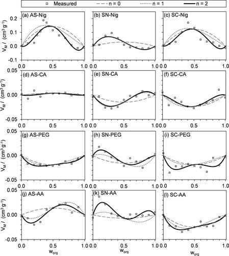
Figure 6. The relative difference in density, δρ, between the best-fit ρ_mix from our non-ideal mixing model (Equations (10)(10) $${\rho }_{\mathrm{mix}}=\frac{1}{\frac{w_{\mathrm{org}}}{{\rho }_{\mathrm{org}}}+\frac{\left({1-w}_{\mathrm{org}}\right)}{{\rho }_{\mathrm{inorg}}}+V_M}$$(10) and (11)(11) $$V_{\mathrm{M}}=w_{\mathrm{org}}\left(1-w_{\mathrm{org}}\right)\sum _{k=0}^n{L}_{\mathrm{k}}{\left(2w_{\mathrm{org}}-1\right)}^k$$(11) ) and the corresponding ideal mixing rule for density (Equation (9)(9) $${\rho }_{\mathrm{ideal}}=\frac{1}{\frac{w_{\mathrm{org}}}{{\rho }_{\mathrm{org}}}+\frac{\left({1-w}_{\mathrm{org}}\right)}{{\rho }_{\mathrm{inorg}}}}$$(9) ) calculated using Equation (13)(13) $$\delta \rho =\frac{{\rho }_{\mathrm{mix}}-{\rho }_{\mathrm{ideal}}}{{\rho }_{\mathrm{ideal}}}·100\mathrm{\%}$$(13) , plotted as a function of organic mass fraction, w_org, for the each of the different organic-inorganic mixtures investigated. The corresponding δρ between the measured ρ_e values and the ideal mixing rule are also shown, with values for AS, SN and SC mixtures shown by square, diamond, and triangle symbols respectively. Note that the vertical scale for (a) is different to that of the other plots.

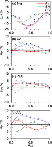
Table 2. The best-fit values of ${\tilde{\rho }}_{\mathrm{org}},$ ${\tilde{\rho }}_{\mathrm{inorg}}$ and the coefficients of the second order RK polynomial describing the measured ρ_e distributions in the organic mass-fraction (w_org) domain according to Equations (10)(10) $${\rho }_{\mathrm{mix}}=\frac{1}{\frac{w_{\mathrm{org}}}{{\rho }_{\mathrm{org}}}+\frac{\left({1-w}_{\mathrm{org}}\right)}{{\rho }_{\mathrm{inorg}}}+V_M}$$(10) and (11)(11) $$V_{\mathrm{M}}=w_{\mathrm{org}}\left(1-w_{\mathrm{org}}\right)\sum _{k=0}^n{L}_{\mathrm{k}}{\left(2w_{\mathrm{org}}-1\right)}^k$$(11) .

Mixture	${\tilde{\rho }}_{\mathrm{org}}$ /(g cm^-3)	${\tilde{\rho }}_{\mathrm{inorg}}$ /(g cm^-3)	L0 /(cm^3 g^-1)	L1 /(cm^3 g^-1)	L2 /(cm^3 g^-1)
AS-Nig	1.606	1.815	0.572	−0.304	−1.003
SN-Nig	1.614	2.237	0.122	−0.473	0.041
SC-Nig	1.596	2.046	0.486	−0.246	−0.764
AS-CA	1.688	1.810	0.014	0.006	−0.032
SN-CA	1.698	2.166	−0.060	0.140	0.031
SC-CA	1.674	2.050	−0.094	0.036	0.091
AS-PEG	1.239	1.808	−0.076	0.035	−0.083
SN-PEG	1.245	2.175	−0.061	−0.110	0.150
SC-PEG	1.236	2.080	−0.075	0.031	−0.245
AS-AA	1.685	1.795	0.055	0.162	−0.146
SN-AA	1.705	2.161	−0.027	−0.100	0.315
SC-AA	1.685	2.061	−0.101	0.065	−0.110

The optimal densities of the organic and inorganic species from our best fits of our non-ideal mixing model are denoted ${\tilde{\rho }}_{\mathrm{org}}$ and ${\tilde{\rho }}_{\mathrm{inorg}},$ respectively, to distinguish these values from our measured values specified in Table 1 that are more robust estimates of the pure component densities.

Figure 6 summarizes the relative deviations in the best-fit ρ_mix from ρ_ideal calculated as: (13) $$\delta \rho =\frac{{\rho }_{\mathrm{mix}}-{\rho }_{\mathrm{ideal}}}{{\rho }_{\mathrm{ideal}}}·100\mathrm{\%}$$(13)

The measured densities deviate from that predicted using an ideal mixing rule model by as much as 20% for mixtures with Nig, compared to no more than 7% for the other mixtures considered. Similarly, Figure S9 shows that the volumes of mixing for mixtures with Nig can be 20–30% of the volumes calculated from ideal mixing contributions, whereas these volumes are no more than 6% for mixtures with the other organic species.

Understanding the trends in non-ideal behavior for mixtures, in general, requires insight into the structure of the material constituting the particle. For example, the organic and inorganic species that, in their pure form, adopt crystalline structures, may form completely different structures when mixed with each other. Even for mixtures of CA in its monohydrate form (which is likely formed following drying at 293 K) and AS, both of which adopt orthorhombic crystal structures (Lafontaine et al. 2013; Okaya et al. 1958), it is not possible to infer straightforwardly the crystal structures; the interactions between CA and the inorganic ions (NH₄⁺, SO₄^-) will be different compared to those between like-species. Even if CA-AS mixtures do crystallize in the orthorhombic system, the unit cell dimensions (therefore deviations from ideal mixture density) are likely different, depending on the strength of the interactions between dissimilar species. Therefore, we cannot predict whether a particular mixture will deviate (and how much by) from ideality based on crystal structure information for pure components. More broadly, we do not have information from this study on whether our particles can be considered as homogeneous, or phase separated.

The specific causes of the highly non-ideal behavior of ρ_e for mixtures containing Nig are unclear. We highlight that the structure and composition of nigrosin dye is not known precisely. For example, Hasenkopf et al. (2010) state that the dye has the chemical formula C₄₉H₂₀N₇S₃O₁₈ which has a molecular weight of 1090.92 g mol⁻¹. Meanwhile, several papers report a chemical formula of C₄₈N₉H₅₁, which has the molecular weight 753.98 g mol⁻¹ (Wiegand et al. 2014; Lack et al. 2006; Bond et al. 1999). Furthermore, the manufacturer for the batch of dye used in our experiments (Sigma-Aldrich) states a molecular weight of 202.21 g mol⁻¹ on their safety data sheet but no chemical formula. Sedlacek and Lee (2007a) describe nigrosin as a mixture of polyaniline pigments with an orange dye. One hypothesis is that the non-ideal behavior for Nig mixtures arises from steric effects, with nigrosin dye containing species with higher molecular weights compared to the inorganic species considered. PEG-400 also has a high molecular weight (380–420 g mol⁻¹) that is probably comparable to that of Nig, but the deviations in ρ_e for PEG mixtures are much less. However, consideration of molecular weight alone does not form a comprehensive assessment of steric effects, as this ignores potential differences in conformational flexibility such as rotational degrees of freedom for the PEG polymeric chains that may be absent in nigrosin species. A second hypothesis is that the aromaticity of the polyaniline species purported to constitute nigrosin dye might strongly influence the intermolecular interactions in the Nig mixtures. However, AA contains a furan ring and yet its mixtures demonstrate relatively mild deviations in ρ_e from ideality, although this observation does not directly exclude the role of the different phenyl aromatic groups that are likely present in nigrosin species in perturbing the volume of mixing.

4.2.3. Non-ideal mixing in the mole fraction domain

The representation of non-ideal mixing in terms of the mass fractions of mixture components can be advantageous because, in our experiments, the masses of individual components are measured directly. This knowledge of mass composition is commonplace in laboratory and field experiments, such as studies that use mass spectrometry. However, the interactions that drive non-ideal mixing occur between molecules and are not physically dependent on masses. Mixtures of two species with equal mass can correspond to vastly different numbers of moles of the two components, depending on their molecular weights. For example, a 1:1 mass mixing ratio of SC:PEG corresponds to a ∼7:1 mole ratio. Therefore, we now consider the representation of ρ_mix in the more physically based mole-fraction domain for all mixtures except those containing nigrosin, as its molecular weight is not known. Although we noted in Section 4.1.2 that the molecular weight of PEG-400 is not known exactly, it is much more constrained (to within ∼5%) than that of nigrosin, and therefore it is reasonable to include densities of the PEG mixtures in the mole-fraction domain.

The ideal mixing rule presented in Equation (9)(9) $${\rho }_{\mathrm{ideal}}=\frac{1}{\frac{w_{\mathrm{org}}}{{\rho }_{\mathrm{org}}}+\frac{\left({1-w}_{\mathrm{org}}\right)}{{\rho }_{\mathrm{inorg}}}}$$(9) for ρ_ideal in terms of mass fractions of the organic species (w_org) can be transformed to an expression in terms of mole fractions of the organic species (x_org): (14) $${\rho }_{\mathrm{ideal}}=\frac{1}{\frac{1}{{\rho }_{\mathrm{inorg}}}\left(\frac{(1-x_{\mathrm{org}})M_{w,\mathrm{inorg}}}{x_{\mathrm{org}}{M}_{w,\mathrm{org}}+\left(1-x_{\mathrm{org}}\right)M_{w,\mathrm{inorg}}}\right)+\frac{1}{{\rho }_{\mathrm{org}}}\left(\frac{x_{\mathrm{org}}{M}_{w,\mathrm{org}}}{x_{\mathrm{org}}{M}_{w,\mathrm{org}}+\left(1-x_{\mathrm{org}}\right)M_{w,\mathrm{inorg}}}\right)}$$(14) in which $M_{w,\mathrm{org}}$ and $M_{w,\mathrm{inorg}}$ are the molecular weights of the organic and inorganic species, respectively. The expression for mixture density is then: (15) $${\rho }_{\mathrm{mix}}=\frac{1}{\frac{1}{{\rho }_{\mathrm{inorg}}}\left(\frac{(1-x_{\mathrm{org}})M_{w,\mathrm{inorg}}}{x_{\mathrm{org}}{M}_{w,\mathrm{org}}+\left(1-x_{\mathrm{org}}\right)M_{w,\mathrm{inorg}}}\right)+\frac{1}{{\rho }_{\mathrm{org}}}\left(\frac{x_{\mathrm{org}}{M}_{w,\mathrm{org}}}{x_{\mathrm{org}}{M}_{w,\mathrm{org}}+\left(1-x_{\mathrm{org}}\right)M_{w,\mathrm{inorg}}}\right)+V_M}$$(15) for which V_M is now expressed as an RK polynomial expansion in terms of the mole fraction: (16) $$V_{\mathrm{M}}=x_{\mathrm{org}}\left(1-x_{\mathrm{org}}\right)\sum _{k=0}^n{L}_{\mathrm{k}}^{\mathrm{\prime }}{\left(2x_{\mathrm{org}}-1\right)}^k$$(16) in which $L_{\mathrm{k}}^{\mathrm{\prime }}$ are the best-fit RK polynomial coefficients when fitting in the mole-fraction domain. We stress that, while Equations (9)(9) $${\rho }_{\mathrm{ideal}}=\frac{1}{\frac{w_{\mathrm{org}}}{{\rho }_{\mathrm{org}}}+\frac{\left({1-w}_{\mathrm{org}}\right)}{{\rho }_{\mathrm{inorg}}}}$$(9) and (14)(14) $${\rho }_{\mathrm{ideal}}=\frac{1}{\frac{1}{{\rho }_{\mathrm{inorg}}}\left(\frac{(1-x_{\mathrm{org}})M_{w,\mathrm{inorg}}}{x_{\mathrm{org}}{M}_{w,\mathrm{org}}+\left(1-x_{\mathrm{org}}\right)M_{w,\mathrm{inorg}}}\right)+\frac{1}{{\rho }_{\mathrm{org}}}\left(\frac{x_{\mathrm{org}}{M}_{w,\mathrm{org}}}{x_{\mathrm{org}}{M}_{w,\mathrm{org}}+\left(1-x_{\mathrm{org}}\right)M_{w,\mathrm{inorg}}}\right)}$$(14) are equivalent and represent the ideal mixing rule in terms of the mass and mole fractions, respectively, of the mixing species, it is important to appreciate that Equations (11)(11) $$V_{\mathrm{M}}=w_{\mathrm{org}}\left(1-w_{\mathrm{org}}\right)\sum _{k=0}^n{L}_{\mathrm{k}}{\left(2w_{\mathrm{org}}-1\right)}^k$$(11) and (16)(16) $$V_{\mathrm{M}}=x_{\mathrm{org}}\left(1-x_{\mathrm{org}}\right)\sum _{k=0}^n{L}_{\mathrm{k}}^{\mathrm{\prime }}{\left(2x_{\mathrm{org}}-1\right)}^k$$(16) for V_M are fundamentally different treatments of the volume of mixing, with the former representing the effects of non-ideal interactions between masses of component species and the latter the effects of interactions between moles of component species. We fit Equations (15)(15) $${\rho }_{\mathrm{mix}}=\frac{1}{\frac{1}{{\rho }_{\mathrm{inorg}}}\left(\frac{(1-x_{\mathrm{org}})M_{w,\mathrm{inorg}}}{x_{\mathrm{org}}{M}_{w,\mathrm{org}}+\left(1-x_{\mathrm{org}}\right)M_{w,\mathrm{inorg}}}\right)+\frac{1}{{\rho }_{\mathrm{org}}}\left(\frac{x_{\mathrm{org}}{M}_{w,\mathrm{org}}}{x_{\mathrm{org}}{M}_{w,\mathrm{org}}+\left(1-x_{\mathrm{org}}\right)M_{w,\mathrm{inorg}}}\right)+V_M}$$(15) and (16)(16) $$V_{\mathrm{M}}=x_{\mathrm{org}}\left(1-x_{\mathrm{org}}\right)\sum _{k=0}^n{L}_{\mathrm{k}}^{\mathrm{\prime }}{\left(2x_{\mathrm{org}}-1\right)}^k$$(16) to our measured densities ρ_e in the same way as before, varying ${\rho }_{\mathrm{org}},$ ${\rho }_{\mathrm{inorg}},$ and $L_{\mathrm{k}}^{\mathrm{\text{'}}}$ to minimize the sums of the relative least-squares residuals. We note that the best fit V_M values still have units of cm³ g⁻¹ (as can be seen from dimensional analysis of Equation (15)(15) $${\rho }_{\mathrm{mix}}=\frac{1}{\frac{1}{{\rho }_{\mathrm{inorg}}}\left(\frac{(1-x_{\mathrm{org}})M_{w,\mathrm{inorg}}}{x_{\mathrm{org}}{M}_{w,\mathrm{org}}+\left(1-x_{\mathrm{org}}\right)M_{w,\mathrm{inorg}}}\right)+\frac{1}{{\rho }_{\mathrm{org}}}\left(\frac{x_{\mathrm{org}}{M}_{w,\mathrm{org}}}{x_{\mathrm{org}}{M}_{w,\mathrm{org}}+\left(1-x_{\mathrm{org}}\right)M_{w,\mathrm{inorg}}}\right)+V_M}$$(15) ), but it is straightforward to convert cm³ g⁻¹ to an excess molar volume with units cm³ mol⁻¹ by dividing by the total number of moles in 1 g of the mixture (which varies with mixture composition). Figure 7 compares our measurements of ρ_e as functions of x_org with the best fits of ρ_mix described by Equations (15)(15) $${\rho }_{\mathrm{mix}}=\frac{1}{\frac{1}{{\rho }_{\mathrm{inorg}}}\left(\frac{(1-x_{\mathrm{org}})M_{w,\mathrm{inorg}}}{x_{\mathrm{org}}{M}_{w,\mathrm{org}}+\left(1-x_{\mathrm{org}}\right)M_{w,\mathrm{inorg}}}\right)+\frac{1}{{\rho }_{\mathrm{org}}}\left(\frac{x_{\mathrm{org}}{M}_{w,\mathrm{org}}}{x_{\mathrm{org}}{M}_{w,\mathrm{org}}+\left(1-x_{\mathrm{org}}\right)M_{w,\mathrm{inorg}}}\right)+V_M}$$(15) and (16)(16) $$V_{\mathrm{M}}=x_{\mathrm{org}}\left(1-x_{\mathrm{org}}\right)\sum _{k=0}^n{L}_{\mathrm{k}}^{\mathrm{\prime }}{\left(2x_{\mathrm{org}}-1\right)}^k$$(16) , with the RK polynomial expression truncated at n = 2 as for our mass mixing comparisons in Sect. 4.2.2. Table 3 summarizes the parameters for the best fits of ρ_mix in the mole fraction domain and the corresponding values of V_M are shown in Figure S10. Across all nine chemical mixtures for which both the mass- and mole-mixing models were fitted, the mean percentage difference between the measured ρ_e and the best-fit models for mass- and mole-mixing took similar values of 3.2% and 3.8%, respectively. Moreover, this percentage difference was lower when using mole mixing for some mixtures (SN with CA, and SC with CA), but was lower when using mass mixing for other mixtures. Therefore, we are unable to distinguish any benefit in using the more physically based mole mixing approach to treating non-ideal interactions for our studies on a limited range of organic-inorganic mixtures.

Figure 7. Measurements of effective density as a function of organic mole fraction (x_org) for internally mixed, two-component particles containing an organic and an inorganic species. The gray squares indicate our measured ρ_e distributions, and the red points are the values that were included in the fit of our non-ideal mixing rule (red lines) in the mole-fraction domain (keeping up to n = 2 in Equation (16)(16) $$V_{\mathrm{M}}=x_{\mathrm{org}}\left(1-x_{\mathrm{org}}\right)\sum _{k=0}^n{L}_{\mathrm{k}}^{\mathrm{\prime }}{\left(2x_{\mathrm{org}}-1\right)}^k$$(16) ; see main text) and represent the best estimate of the effective density at a given w_org by including all data from repeat measurements in a single regression of $d_{\mathrm{ae}}^2{C}_{\mathrm{c}}\left(d_{\mathrm{ae}}\right)$ versus $d_{\mathrm{m}}^2{C}_{\mathrm{c}}\left(d_{\mathrm{m}}\right).$ The blue dashed line is the ideal mixing rule prediction (Equation (15)(15) $${\rho }_{\mathrm{mix}}=\frac{1}{\frac{1}{{\rho }_{\mathrm{inorg}}}\left(\frac{(1-x_{\mathrm{org}})M_{w,\mathrm{inorg}}}{x_{\mathrm{org}}{M}_{w,\mathrm{org}}+\left(1-x_{\mathrm{org}}\right)M_{w,\mathrm{inorg}}}\right)+\frac{1}{{\rho }_{\mathrm{org}}}\left(\frac{x_{\mathrm{org}}{M}_{w,\mathrm{org}}}{x_{\mathrm{org}}{M}_{w,\mathrm{org}}+\left(1-x_{\mathrm{org}}\right)M_{w,\mathrm{inorg}}}\right)+V_M}$$(15) ). Note that the different rows of plots have differing vertical scale value ranges.

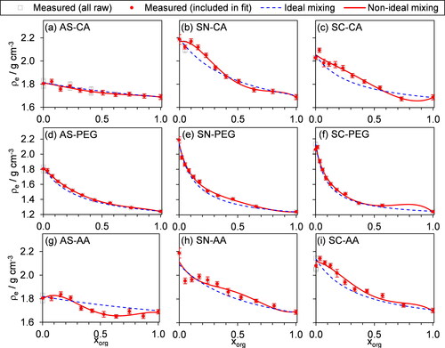
Table 3. The best-fit values of ${\tilde{\rho }}_{\mathrm{org}},$ ${\tilde{\rho }}_{\mathrm{inorg}}$ and the first and second order coefficients of the RK polynomial describing the measured ρ_e distributions in the organic mole-fraction (x_org) domain according to Equations (15)(15) $${\rho }_{\mathrm{mix}}=\frac{1}{\frac{1}{{\rho }_{\mathrm{inorg}}}\left(\frac{(1-x_{\mathrm{org}})M_{w,\mathrm{inorg}}}{x_{\mathrm{org}}{M}_{w,\mathrm{org}}+\left(1-x_{\mathrm{org}}\right)M_{w,\mathrm{inorg}}}\right)+\frac{1}{{\rho }_{\mathrm{org}}}\left(\frac{x_{\mathrm{org}}{M}_{w,\mathrm{org}}}{x_{\mathrm{org}}{M}_{w,\mathrm{org}}+\left(1-x_{\mathrm{org}}\right)M_{w,\mathrm{inorg}}}\right)+V_M}$$(15) and (16)(16) $$V_{\mathrm{M}}=x_{\mathrm{org}}\left(1-x_{\mathrm{org}}\right)\sum _{k=0}^n{L}_{\mathrm{k}}^{\mathrm{\prime }}{\left(2x_{\mathrm{org}}-1\right)}^k$$(16) .

Mixture	${\tilde{\rho }}_{\mathrm{org}}$ /(g cm^-3)	${\tilde{\rho }}_{\mathrm{inorg}}$ /(g cm^-3)	$L_0^{\mathrm{\prime }}$ /(cm^3 g^-1)	$L_1^{\mathrm{\prime }}$ /(cm^3 g^-1)	$L_2^{\mathrm{\prime }}$ /(cm^3 g^-1)
AS-CA	1.688	1.811	0.015	−0.005	−0.028
SN-CA	1.688	2.165	0.001	0.110	−0.253
SC-CA	1.688	2.055	−0.028	0.190	0.043
AS-PEG	1.240	1.820	−0.043	0.059	−0.141
SN-PEG	1.240	2.142	−0.085	0.096	0.117
SC-PEG	1.241	2.121	−0.034	−0.142	−0.474
AS-AA	1.682	1.799	0.076	0.119	−0.209
SN-AA	1.695	2.113	−0.048	−0.001	0.176
SC-AA	1.699	2.117	−0.039	0.065	−0.197

The optimal densities of the organic and inorganic species from our best fits of our non-ideal mixing model are denoted ${\tilde{\rho }}_{\mathrm{org}}$ and ${\tilde{\rho }}_{\mathrm{inorg}},$ respectively, to distinguish these values from our measured values specified in Table 1 that are more robust estimates of the pure component densities.

The magnitudes of the excess molar volumes for our nanoparticle solid-solid (and solid-liquid in the case of PEG) mixtures are up to 4 cm³ mol⁻¹. To the best of our knowledge, little (if any) research has focused on mixture densities for dry, solid particles, although many investigations have reported excess molar volumes for liquids including aqueous solutions (Rodríguez et al. 2012; Clegg and Wexler 2011) and ionic liquids (Singh et al. 2009). Values of V_M in aqueous solutions and ionic liquids are typically less than 1 cm³ mol⁻¹, so the excess molar volumes observed in our study indicate appreciable non-ideal mixing in solids.

5. Conclusions

We have applied the AAC-SMPS approach to the determination of effective densities for two component organic-inorganic mixtures and considered how various factors impacted the accuracy of this determination. Uncertainties in the particle aerodynamic and mobility diameters and differences in formulations of the Cunningham slip correction factor could introduce biases in determined ρ_e of up to ±3.8%, ±4.2%, and ∼0.3%, respectively. An analysis of the particle mass-mobility exponent (f) indicates that ρ_e is independent of particle size and therefore the assumption of size-independent densities is valid. Importantly, our measured ρ_e for single component aerosols comprised of nonvolatile (solid) materials agreed to within ∼5% of the known material densities available in the literature. Deviations in ρ_e from known material densities occurred when the particles contained a semi-volatile component; these situations are attributed to reductions in the particle mobility diameters between AAC classification and measurements of the particle mobility diameter distributions due to evaporation. Researchers should take care in ensuring that any impacts of volatility of their aerosol samples are considered if using the AAC-SMPS approach for effective density characterization. Furthermore, we have shown that the precision in our measured ρ_e values is ∼1%.

Our effective density measurements for two-component organic-inorganic mixtures demonstrated substantial deviations from expectations of an ideal mixing model, except for AS-CA mixtures. We utilized two different approaches to modeling the non-ideal mixing for our systems, both of which used Redlich-Kister polynomials to represent the volume change of mixing: one model parameterized the mixing in terms of mass fractions (i.e., it treated the mixing between component masses), whereas the other model parameterized the mixing in terms of mole fractions (i.e., it treated the mixing between molecules). We could not distinguish any significant difference in the performance of the more physically based mole-mixing approach over the treatment of non-ideal mixing between masses. Ultimately, deviations in density from ideal mixing were up to 20% for mixtures involving nigrosin dye, and up to 7% for those containing the other organics investigated. Excess molar volumes for our dry particles (neglecting those comprising nigrosin) were up to 4 cm³ mol⁻¹, which is substantially larger than the excess molar volumes reported for common aqueous or ionic liquid mixtures. The large deviations in ρ_e from ideal mixing reported here likely have great impacts on current common approaches for estimating effective densities from mass spectrometry data, and on predictions of parameters that depend on effective density. The assumption of ideal mixing could introduce considerable biases in predictions of densities, with subsequent impacts on the calculation of aerosol dynamical and optical properties.

Disclosure statement

The authors declare that they have no conflict of interest.

Data availability

For data related to this article, please contact Michael I. Cotterell ([email protected]).

Additional information

Funding

Elinor T. Vokes was supported through a studentship provided by the Engineering and Physical Sciences Research Council (EPSRC) Center for Doctoral training in Aerosol Science (EP/S023593/1). Michael I. Cotterell acknowledges the support of the Natural Environment Research Council through an Independent Research Fellowship (NE/S014314/1). Ernie R. Lewis was supported by the Scientific Focus Area Science Plan program that is supported by the Office of Biological and Environmental Research in the Department of Energy, Office of Science, through the United States Department of Energy Contract No. DE-SC0012704 to Brookhaven National Laboratory. We thank the EPSRC for funding the purchase of the AAC and CPC used in this work through a Core Equipment Grant (EP/V036440/1). We also acknowledge Dr Bryan Bzdek (University of Bristol) for securing a further EPSRC Core Equipment Grant (EP/S018050/1) that funded the purchase of the aerosol mobility classifier used in this work.

References

- Allen, M. D., and O. G. Raabe. 1985. Slip correction measurements of spherical solid aerosol particles in an improved Millikan apparatus. Aerosol Sci. Technol. 4 (3):269–86. doi:10.1080/02786828508959055.
- Allen, M. D., and O. G. Raabe. 1982. Re-evaluation of Millikan’s oil drop data for the motion of small particles in air. J. Aerosol Sci. 13 (6):537–47. doi:10.1016/0021-8502(82)90019-2.
- Ashcroft, S. J., D. R. Booker, and J. Turner. 1990. Density measurement by oscillating tube. Effects of viscosity, temperature, calibration and signal processing. Faraday Trans. 86 (1):145. doi:10.1039/ft9908600145.
- Baldelli, A., and R. Vehring. 2016. Analysis of cohesion forces between monodisperse microparticles with rough surfaces. Colloids Surfaces A Physicochem. Eng. Asp. 506:179–89. doi:10.1016/j.colsurfa.2016.06.009.
- Bannan, T. J., M. Le Breton, M. Priestley, S. D. Worrall, A. Bacak, N. A. Marsden, A. Mehra, J. Hammes, M. Hallquist, M. R. Alfarra, et al. 2019. A method for extracting calibrated volatility information from the FIGAERO-HR-ToF-CIMS and its experimental application. Atmos. Meas. Tech. 12 (3):1429–39. doi:10.5194/amt-12-1429-2019.
- Baxter, G. P., and C. C. Wallace. 1916. The densities and cubical coefficients of expansion of the halogen salts of sodium, potassium, rubidium and cesium. J. Am. Chem. Soc. 38 (2):259–66. doi:10.1021/ja02259a009.
- Bennett, G. M., and J. L. Yuill. 1935. The crystal form of anhydrous citric acid. J. Chem. Soc. 1935 (130):130. doi:10.1039/jr9350000130.
- Bilde, M., K. Barsanti, M. Booth, C. D. Cappa, N. M. Donahue, E. U. Emanuelsson, G. McFiggans, U. K. Krieger, C. Marcolli, D. Topping, et al. 2015. Saturation vapor pressures and transition enthalpies of low-volatility organic molecules of atmospheric relevance: From dicarboxylic acids to complex mixtures. Chem. Rev. 115 (10):4115–56. doi:10.1021/cr5005502.
- Bond, T. C., T. L. Anderson, and D. Campbell. 1999. Calibration and intercomparison of filter-based measurements of visible light absorption by aerosols. Aerosol Sci. Technol. 30 (6):582–600. doi:10.1080/027868299304435.
- Brockmann, J. E., and D. J. Rader. 1990. APS response to nonspherical particles and experimental determination of dynamic shape factor. Aerosol Sci. Technol. 13 (2):162–72. doi:10.1080/02786829008959434.
- Bzdek, B. R., J. P. Reid, and M. I. Cotterell. 2020. Open questions on the physical properties of aerosols. Commun. Chem. 3 (1):105.
- Cai, C., R. Miles, M. I. Cotterell, A. Marsh, G. Rovelli, A. Rickards, Y. Zhang, and J. P. Reid. 2016. Comparison of methods for predicting the compositional dependence of the density and refractive index of organic–Aqueous aerosols. J. Phys. Chem. A 120 (33):6604–17.
- Cai, C., D. J. Stewart, J. P. Reid, Y. Zhang, P. Ohm, C. S. Dutcher, and S. L. Clegg. 2015. Organic component vapor pressures and hygroscopicities of aqueous aerosol measured by optical tweezers. J. Phys. Chem. A 119 (4):704–18. doi:10.1021/jp510525r.
- Cappa, C. D., D. A. Lack, J. B. Burkholder, and A. R. Ravishankara. 2008. Bias in filter-based aerosol light absorption measurements due to organic aerosol loading: evidence from laboratory measurements. Aerosol Sci. Technol. 42 (12):1022–32. doi:10.1080/02786820802389285.
- Choczynski, J. M., R. Kaur Kohli, C. S. Sheldon, C. L. Price, and J. F. Davies. 2021. A dual-droplet approach for measuring the hygroscopicity of aqueous aerosol. Atmos. Meas. Tech. 14 (7):5001–13. doi:10.5194/amt-14-5001-2021.
- Clegg, S. L., and A. S. Wexler. 2011. Densities and apparent molar volumes of atmospherically important electrolyte solutions. 1. the solutes H2SO4, HNO 3, HCl, Na2SO4, NaNO3, NaCl, (NH4)2SO4, NH4NO3, and NH4Cl from 0 to 50 °C. J. Phys. Chem. A 115 (15):3393–460. doi:10.1021/jp108992a.
- Cotterell, M. I., B. J. Mason, A. E. Carruthers, J. S. Walker, A. J. Orr-Ewing, and J. P. Reid. 2014. Measurements of the evaporation and hygroscopic response of single fine-mode aerosol particles using a Bessel beam optical trap. Phys. Chem. Chem. Phys. 16 (5):2118–28.
- Cotterell, M. I., K. Szpek, J. M. Haywood, and J. M. Langridge. 2020. Sensitivity and accuracy of refractive index retrievals from measured extinction and absorption cross sections for mobility-selected internally mixed light absorbing aerosols. Aerosol Sci. Technol. 54 (9):1034–57. doi:10.1080/02786826.2020.1757034.
- Cotterell, M. I., R. E. Willoughby, B. R. Bzdek, A. J. Orr-Ewing, and J. P. Reid. 2017. A complete parameterisation of the relative humidity and wavelength dependence of the refractive index of hygroscopic inorganic aerosol particles. Atmos. Chem. Phys. 17 (16):9837–51. doi:10.5194/acp-17-9837-2017.
- Cross, E. S., T. B. Onasch, A. Ahern, W. Wrobel, J. G. Slowik, J. Olfert, D. A. Lack, P. Massoli, C. D. Cappa, J. P. Schwarz, et al. 2010. Soot particle studies-instrument inter-comparison-project overview. Aerosol Sci. Technol. 44 (8):592–611. doi:10.1080/02786826.2010.482113.
- Davies, C. N. 1945. Definitive equations for the fluid resistance of spheres. Proc. Phys. Soc. 57 (4):259–70.
- Davies, N. W., M. I. Cotterell, C. Fox, K. Szpek, J. M. Haywood, and J. M. Langridge. 2018. On the accuracy of aerosol photoacoustic spectrometer calibrations using absorption by ozone. Atmos. Meas. Tech. 11 (4):2313–24. doi:10.5194/amt-11-2313-2018.
- Davies, N. W., C. Fox, K. Szpek, M. I. Cotterell, J. W. Taylor, J. D. Allan, P. I. Williams, J. Trembath, J. M. Haywood, and J. M. Langridge. 2019. Evaluating biases in filter-based aerosol absorption measurements using photoacoustic spectroscopy. Atmos. Meas. Tech. 12 (6):3417–34. doi:10.5194/amt-12-3417-2019.
- DeCarlo, P. F., J. G. Slowik, D. R. Worsnop, P. Davidovits, and J. L. Jimenez. 2004. Particle morphology and density characterization by combined mobility and aerodynamic diameter measurements. Part 1: Theory. Aerosol Sci. Technol. 38 (12):1185–205. doi:10.1080/027868290903907.
- Edwards, D. A., A. Ben-Jebria, and R. Langer. 1998. Recent advances in pulmonary drug delivery using large, porous inhaled particles. J. Appl. Physiol. (1985) 85 (2):379–85.
- Edwards, D. A., Hanes, J. Caponetti, G. Hrkach, J. Ben-Jebria, A. Eskew, M. Lou, Mintzes, J. Deaver, D. Lotan, N. Langer, R, et al. 1997. Large porous particles for pulmonary drug delivery. Science 276 (5320):1868–71. doi:10.1126/science.276.5320.1868.
- Edwards, J. M., and A. Slingo. 1996. Studies with a flexible new radiation code. I: Choosing a configuration for a large-scale model. QJ. R. Met. Soc. 122 (531):689–719. doi:10.1002/qj.49712253107.
- Eggersdorfer, M. L., A. J. Gröhn, C. M. Sorensen, P. H. McMurry, and S. E. Pratsinis. 2012. Mass-mobility characterization of flame-made ZrO 2 aerosols: Primary particle diameter and extent of aggregation. J. Colloid Interface Sci. 387 (1):12–23.
- Hardy, D. A., J. Archer, P. Lemaitre, R. Vehring, J. P. Reid, and J. S. Walker. 2021. High time resolution measurements of droplet evaporation kinetics and particle crystallisation. Phys. Chem. Chem. Phys. 23 (34):18568–79. doi:10.1039/D1CP02840E.
- Hasenkopf, C. A., M. R. Beaver, M. G. Trainer, H. Langley Dewitt, M. A. Freedman, O. B. Toon, C. P. McKay, and M. A. Tolbert. 2010. Optical properties of Titan and early Earth haze laboratory analogs in the mid-visible. Icarus 207 (2):903–13. doi:10.1016/j.icarus.2009.12.015.
- Haywood, J. M., S. J. Abel, P. A. Barrett, N. Bellouin, A. Blyth, K. N. Bower, M. Brooks, K. Carslaw, H. Che, H. Coe, et al. 2021. The cloud – Aerosol – Radiation interaction and forcing : Year 2017 (CLARIFY-2017) measurement campaign. Atmos. Chem. Phys. 21 (1):1049–84.
- Hinds, W. C. 1999. Aerosol technology: properties, behavior, and measurement of airborne particles, 2nd ed. New York: Wiley.
- Hu, D., M. R. Alfarra, K. Szpek, J. Langridge, M. Cotterell, C. Belcher, I. Rule, Z. Liu, C. Yu, Y. Shao, et al. 2021. Physical and chemical properties of black carbon and organic matter from different sources using aerodynamic aerosol classification. Atmos. Chem. Phys. 21 (21): 1–50. doi:10.5194/acp-21-16161-2021.
- Johnson, T. J., M. Irwin, J. Symonds, J. S. Olfert, and A. M. Boies. 2018. Measuring aerosol size distributions with the aerodynamic aerosol classifier. Aerosol Sci. Technol. 52 (6):655–65. doi:10.1080/02786826.2018.1440063.
- Johnson, T. J., R. T. Nishida, M. Irwin, J. Symonds, J. S. Olfert, and A. M. Boies. 2020. Measuring the bipolar charge distribution of nanoparticles: Review of methodologies and development using the Aerodynamic Aerosol Classifier. J. Aerosol Sci. 143:105526. (doi:10.1016/j.jaerosci.2020.105526.
- Johnston, H. L., and D. A. Hutchison. 1942. Density of sodium chloride – The atomic weight of fluorine by combination of crystal density and X-ray data. Phys. Rev. 62 (1-2):32–6. doi:10.1103/PhysRev.62.32.
- Johnston, J., and L. H. Adams. 1912. On the density of solid substances with especial reference to permanent changes produced by high pressures. J. Am. Chem. Soc. 34 (5):563–84. doi:10.1021/ja02206a001.
- Kim, J. H., G. W. Mulholland, S. R. Kukuck, and D. Pui. 2005. Slip correction measurements of certified PSL nanoparticles using a nanometer differential mobility analyzer (Nano-DMA) for knudsen number from 0.5 to 83. J. Res. Natl. Inst. Stand. Technol. 110 (1):31–54.
- Kinney, P. D., D. Pui, G. W. Mulholland, and N. P. Bryner. 1991. Use of the electrostatic classification method to size 0.1 micrometer SRM particles – A feasibility study. J. Res. Natl. Inst. Stan. 96 (2):147. doi:10.6028/jres.096.006.
- Kracek, F. C. 1931. Gradual transition in sodium nitrate. I. physico-chemical criteria of the transition. J. Am. Chem. Soc. 53 (7):2609–24. doi:10.1021/ja01358a022.
- Krieger, U. K., C. Marcolli, and J. P. Reid. 2012. Exploring the complexity of aerosol particle properties and processes using single particle techniques. Chem. Soc. Rev. 41 (19):6631–62.
- Krieger, U. K., F. Siegrist, C. Marcolli, E. U. Emanuelsson, F. M. Gøbel, M. Bilde, A. Marsh, J. P. Reid, A. J. Huisman, I. Riipinen, et al. 2018. A reference data set for validating vapor pressure measurement techniques: homologous series of polyethylene glycols. Atmos. Meas. Tech. 11 (1):49–63. doi:10.5194/amt-11-49-2018.
- Kuramoto, N., K. Fujii, and A. Waseda. 2004. Accurate density measurements of reference liquids by a magnetic suspension balance. Metrologia 41 (2):S84–S94. doi:10.1088/0026-1394/41/2/S09.
- Lack, D. A., E. R. Lovejoy, T. Baynard, A. Pettersson, and A. R. Ravishankara. 2006. Aerosol absorption measurement using photoacoustic spectroscopy: Sensitivity, calibration, and uncertainty developments. Aerosol Sci. Technol. 40 (9):697–708. doi:10.1080/02786820600803917.
- Lafontaine, A., M. Sanselme, Y. Cartigny, P. Cardinael, and G. Coquerel. 2013. Characterization of the transition between the monohydrate and the anhydrous citric acid. J. Therm. Anal. Calorim. 112 (1):307–15. doi:10.1007/s10973-012-2798-0.
- Langridge, J. M., M. S. Richardson, D. A. Lack, and D. M. Murphy. 2016. Experimental evidence supporting the insensitivity of cloud droplet formation to the mass accommodation coefficient for condensation of water vapor to liquid water. Geophys. Res. Lett. 43 (12):6650–6. doi:10.1002/2016GL069328.
- Leppä, J., W. Mui, A. M. Grantz, and R. C. Flagan. 2017. Charge distribution uncertainty in differential mobility analysis of aerosols. Aerosol Sci. Technol. 51 (10):1168–89. doi:10.1080/02786826.2017.1341039.
- Lienhard, D. M., D. L. Bones, A. Zuend, U. K. Krieger, J. P. Reid, and T. Peter. 2012. Measurements of thermodynamic and optical properties of selected aqueous organic and organic–inorganic mixtures of atmospheric relevance. J. Phys. Chem. A 116 (40):9954–68.
- Liu, Y., and P. H. Daum. 2008. Relationship of refractive index to mass density and self-consistency of mixing rules for multicomponent mixtures like ambient aerosols. J. Aerosol Sci. 39 (11):974–86. doi:10.1016/j.jaerosci.2008.06.006.
- Logozzo, A., and T. C. Preston. 2021. Temperature-controlled dual-beam optical trap for single particle studies of organic aerosol. J. Phys. Chem. A. 126:109–118.
- Marshall, F. H., R. Miles, Y.-C. Song, P. B. Ohm, R. M. Power, J. P. Reid, and C. S. Dutcher. 2016. Diffusion and reactivity in ultraviscous aerosol and the correlation with particle viscosity. Chem. Sci. 7 (2):1298–308.
- Mason, B. J., M. I. Cotterell, T. C. Preston, A. J. Orr-Ewing, and J. P. Reid. 2015. Direct measurements of the optical cross sections and refractive indices of individual volatile and hygroscopic aerosol particles. J. Phys. Chem. A 119 (22):5701–13.
- McMurry, P. H., X. Wang, K. Park, and K. Ehara. 2002. The relationship between mass and mobility for atmospheric particles: A new technique for measuring particle density. Aerosol Sci. Technol. 36 (2):227–38. doi:10.1080/027868202753504083.
- Moteki, N., Y. Kondo, T. Nakayama, K. Kita, L. K. Sahu, T. Ishigai, T. Kinase, and Y. Matsumi. 2010. Radiative transfer modeling of filter-based measurements of light absorption by particles: Importance of particle size dependent penetration depth. J. Aerosol Sci. 41 (4):401–12. doi:10.1016/j.jaerosci.2010.02.002.
- Murphy, D. M., D. J. Cziczo, K. D. Froyd, P. K. Hudson, B. M. Matthew, A. M. Middlebrook, R. E. Peltier, A. Sullivan, D. S. Thomson, and R. J. Weber. 2006. Single-particle mass spectrometry of tropospheric aerosol particles. J. Geophys. Res. 111 (D23):1–15. doi:10.1029/2006JD007340.
- Murray, B. J. 2008. Inhibition of ice crystallisation in highly viscous aqueous organic acid droplets. Atmos. Chem. Phys. 8 (17):5423–33. doi:10.5194/acp-8-5423-2008.
- Okaya, Y., K. Vedam, and R. Pepinsky. 1958. Non-isomorphism of ferroelectric phases of ammonium sulfate and ammonium fluoberyllate. Acta Cryst. 11 (4):307– doi:10.1107/S0365110X58000803.
- Olfert, J., and S. Rogak. 2019. Universal relations between soot effective density and primary particle size for common combustion sources. Aerosol Sci. Technol. 53 (5):485–92. doi:10.1080/02786826.2019.1577949.
- Pagels, J., A. F. Khalizov, P. H. McMurry, and R. Y. Zhang. 2009. Processing of soot by controlled sulphuric acid and water condensation—Mass and mobility relationship. Aerosol Sci. Technol. 43 (7):629–40. doi:10.1080/02786820902810685.
- Peng, L., Z. Li, G. Zhang, X. Bi, W. Hu, M. Tang, X. Wang, P. Peng, and G. Sheng. 2021. A review of measurement techniques for aerosol effective density. Sci. Total Environ. 778:146248.
- Pistone, K., J. Redemann, S. Doherty, P. Zuidema, S. Burton, B. Cairns, S. Cochrane, R. Ferrare, C. Flynn, S. Freitag, et al. 2019. Intercomparison of biomass burning aerosol optical properties from in situ and remote-sensing instruments in ORACLES-2016. Atmos. Chem. Phys. 19 (14):9181–208. doi:10.5194/acp-19-9181-2019.
- Pokhrel, R. P., J. Gordon, M. N. Fiddler, and S. Bililign. 2021. Impact of combustion conditions on physical and morphological properties of biomass burning aerosol. Aerosol Sci. Technol. 55 (1):80–91. doi:10.1080/02786826.2020.1822512.
- Pusz, S., M. Krzesińska, Ł. Smędowski, J. Majewska, B. Pilawa, and B. Kwiecińska. 2010. Changes in a coke structure due to reaction with carbon dioxide. Int. J. Coal Geol 81 (4):287–92. doi:10.1016/j.coal.2009.07.013.
- Radney, J. G., and C. D. Zangmeister. 2018. Comparing aerosol refractive indices retrieved from full distribution and size- and mass-selected measurements. J. Quant. Spectrosc. Radiat. Transf. 220:52–66. doi:10.1016/j.jqsrt.2018.08.021.
- Radney, J. G., and C. D. Zangmeister. 2015. Measurement of gas and aerosol phase absorption spectra across the visible and near-IR using supercontinuum photoacoustic spectroscopy. Anal. Chem. 87 (14):7356–63. doi:10.1021/acs.analchem.5b01541.
- Ray, A. K., R. D. Johnson, and A. Souyri. 1989. Dynamic behavior of single glycerol droplets in humid air streams. Langmuir 5 (1):133–40. doi:10.1021/la00085a024.
- Redemann, J., R. Wood, P. Zuidema, S. J. Doherty, B. Luna, S. E. LeBlanc, M. S. Diamond, Y. Shinozuka, I. Y. Chang, R. Ueyama, et al. 2021. An overview of the ORACLES (ObseRvations of Aerosols above CLouds and their intEractionS) project: Aerosol–cloud–radiation interactions in the southeast Atlantic basin. Atmos. Chem. Phys. 21 (3):1507–63. doi:10.5194/acp-21-1507-2021.
- Redlich, O., and A. T. Kister. 1948. Algebraic representation of thermodynamic properties and the classification of solutions. Ind. Eng. Chem. 40 (2):345–8. doi:10.1021/ie50458a036.
- Riemer, N., A. P. Ault, M. West, R. L. Craig, and J. H. Curtis. 2019. Aerosol mixing state: measurements, modeling, and impacts. Rev. Geophys. 57 (2):187–249. doi:10.1029/2018RG000615.
- Robie, R., P. Bethke, and K. Beardsley. 1967. Selected X-ray crystallographic data, molar volumes, and densities of minerals and related substances. US Geol. Surv. Bull. (1248):1–87. doi:10.3133/b1248.
- Rodríguez, G. A., A. R. Holguín, F. Martínez, M. Khoubnasabjafari, and A. Jouyban. 2012. Volumetric properties of (PEG 400 + water) and (PEG 400 + ethanol) mixtures at several temperatures and correlation with the Jouyban-Acree model. Rev. Colomb. Ciencias Químico – Farm 41:187–202.
- Sedlacek, A., and J. Lee. 2007. Photothermal interferometric aerosol absorption spectrometry. Aerosol Sci. Technol. 41 (12):1089–101. doi:10.1080/02786820701697812.
- Sequeira, M., M. Pereira, H. Avelino, F. Caetano, and J. Fareleira. 2019. Viscosity measurements of poly(ethyleneglycol) 400 [PEG 400] at temperatures from 293 K to 348 K and at pressures up to 50 MPa using the vibrating wire technique. Fluid Phase Equilib. 496:7–16. doi:10.1016/j.fluid.2019.05.012.
- Singh, T., A. Kumar, M. Kaur, G. Kaur, and H. Kumar. 2009. Non-ideal behaviour of imidazolium based room temperature ionic liquids in ethylene glycol at T = (298.15 to 318.15) K. J. Chem. Thermodyn. 41 (6):717–23. doi:10.1016/j.jct.2008.12.002.
- Sonnergaard, J. 2000. Impact of particle density and initial volume on mathematical compression models. Eur. J. Pharm. Sci. 11 (4):307–15.
- Stolzenburg, M. R., and P. H. McMurry. 2008. Equations governing single and tandem DMA configurations and a new lognormal approximation to the transfer function. Aerosol Sci. Technol. 42 (6):421–32. doi:10.1080/02786820802157823.
- Swanson, H. E., N. T. Gilfrich, and M. Cook. 1956. Standard X-ray diffraction powder patterns. Natl. Bur. Stand. Circ. 6 (539):1–68. doi:10.6028/NBS.CIRC.539v6.
- Tang, IN., and H. R. Munkelwitz. 1994. Water activities, densities, and refractive indices of aqueous sulfates and sodium nitrate droplets of atmospheric importance. J. Geophys. Res. 99 (D9):18801. doi:10.1029/94JD01345.
- Tang, IN., A. C. Tridico, and K. H. Fung. 1997. Thermodynamic and optical properties of sea salt aerosols. J. Geophys. Res. 102 (D19):23269–75. doi:10.1029/97JD01806.
- Tavakoli, F., and J. S. Olfert. 2014. Determination of particle mass, effective density, mass–mobility exponent, and dynamic shape factor using an aerodynamic aerosol classifier and a differential mobility analyzer in tandem. J. Aerosol Sci. 75:35–42. doi:10.1016/j.jaerosci.2014.04.010.
- Tavakoli, F., and J. S. Olfert. 2013. An instrument for the classification of aerosols by particle relaxation time: Theoretical models of the aerodynamic aerosol classifier. Aerosol Sci. Technol 47 (8):916–26. doi:10.1080/02786826.2013.802761.
- Tavakoli, F., J. Symonds, and J. S. Olfert. 2014. Generation of a monodisperse size-classified aerosol independent of particle charge. Aerosol Sci. Technol. 48 (3):i–iv. doi:10.1080/02786826.2013.877121.
- Taylor, J. W., H. Wu, K. Szpek, K. Bower, I. Crawford, M. J. Flynn, P. I. Williams, J. Dorsey, J. M. Langridge, M. I. Cotterell, et al. 2020. Absorption closure in highly aged biomass burning smoke. Atmos. Chem. Phys. 20 (19):11201–21. doi:10.5194/acp-20-11201-2020.
- Tigges, L., A. Jain, and H. J. Schmid. 2015a. On the bipolar charge distribution used for mobility particle sizing: Theoretical considerations. J. Aerosol Sci. 88:119–34. doi:10.1016/j.jaerosci.2015.05.010.
- Tigges, L., A. Wiedensohler, K. Weinhold, J. Gandhi, and H. J. Schmid. 2015b. Bipolar charge distribution of a soft X-ray diffusion charger. J. Aerosol Sci. 90:77–86. doi:10.1016/j.jaerosci.2015.07.002.
- Tutton, A. 1906. Ammonium selenate and the question of isodimorphism in the alkali series. J. Chem. Soc. Trans. 89 (0):1059–83. doi:10.1039/CT9068901059.
- Wagner, W., and R. Kleinrahm. 2004. Densimeters for very accurate density measurements of fluids over large ranges of temperature, pressure, and density. Metrologia 41 (2):S24–S39. doi:10.1088/0026-1394/41/2/S03.
- Walker, J. S., J. Archer, F. Gregson, S. Michel, B. R. Bzdek, and J. P. Reid. 2021. Accurate representations of the microphysical processes occurring during the transport of exhaled aerosols and droplets. ACS Cent. Sci. 7 (1):200–9. doi:10.1021/acscentsci.0c01522.
- Wang, B., and A. Laskin. 2014. Reactions between water-soluble organic acids and nitrates in atmospheric aerosols: Recycling of nitric acid and formation of organic salts. J. Geophys. Res. Atmos. 119 (6):3335–51. doi:10.1002/2013JD021169.
- Wiegand, J. R., L. D. Mathews, and G. D. Smith. 2014. A UV-vis photoacoustic spectrophotometer. Anal. Chem. 86 (12):6049–56.
- Wu, H., J. W. Taylor, J. M. Langridge, C. Yu, J. D. Allan, K. Szpek, M. I. Cotterell, P. I. Williams, M. Flynn, P. Barker, et al. 2021. Rapid transformation of ambient absorbing aerosols from West African biomass burning. Atmos. Chem. Phys. 21 (12):9417–40. doi:10.5194/acp-21-9417-2021.
- Zardini, A. A., I. Riipinen, I. K. Koponen, M. Kulmala, and M. Bilde. 2010. Evaporation of ternary inorganic/organic aqueous droplets: Sodium chloride, succinic acid and water. J. Aerosol Sci. 41 (8):760–70. doi:10.1016/j.jaerosci.2010.05.003.
- Zelenyuk, A., Y. Cai, and D. Imre. 2006. From agglomerates of spheres to irregularly shaped particles: Determination of dynamic shape factors from measurements of mobility and vacuum aerodynamic diameters. Aerosol Sci. Technol. 40 (3):197–217. doi:10.1080/02786820500529406.