Effect of a barrier on spatial distribution of respiratory particles in a room

Abstract

Barriers have been widely used to mitigate transmission of Covid-19 and other diseases. Their efficacy for aerosol particles is not well established. The objective of this study was to quantify the impact of a barrier on the spatial distribution of particles released by speaking in a room with a low air-change rate (0.6 ± 0.2 h⁻¹). The source was a nebulizer that released fluorescent microspheres of diameters 0.5, 1, 6, 10, or 20 µm for 20 min, and the room was outfitted with 108 passive sampling sites. We counted the number of microspheres deposited on slides at sampling locations after >1 h. The presence of a barrier 0.46 m in front of the source resulted in an increase in 0.5 µm particles deposited on the source-side of the barrier and an increase in 0.5 µm particles around the sides of the barrier laterally and at certain locations 4–6 m from the source. The barrier had a minor effect on the distribution of 1 µm particles. There was no observable effect of the barrier on the distribution of 6, 10, and 20 µm particles. Most 10 and 20 µm particles deposited within 0.3 m of the source, although some were found at locations >3 m from the source. These results indicate that barriers may not serve as adequate protection to others in the room, depending on their location relative to the barrier and the exposure timescale. A limitation is that our study utilized only one barrier configuration at one air-change rate.

EDITOR:

• Shanna Ratnesar-Shumate

Introduction

In response to the Covid-19 pandemic, physical barriers have been erected in many public spaces in an attempt to reduce the risk of transmission of SARS-CoV-2, although there have been little guidance as to how barriers should be implemented and limited evidence of their effectiveness. SARS-CoV-2 spreads when an infected person releases respiratory droplets or aerosol particles containing the virus, and a susceptible individual is exposed to the virus via inhalation or contact with the mucus membranes of the nose, eyes, or mouth (Centers for Disease Control and Prevention 2021). Studies have shown that most respiratory particles generated while breathing are <1 µm. Those generated while coughing or speaking range in size from <0.1 µm to >20 µm. The majority of speech-generated particles are <6 µm, although the details of the size distribution depend on consonants and speech patterns (Morawska et al. 2009; Asadi et al. 2019; Lee et al. 2019; Lindsley et al. 2012; Shen et al. 2022). SARS-CoV-2 has a diameter of about 0.1 µm and has been detected in particles spanning a wide range of sizes, from <0.25 to >4 µm in hospital and residential settings (Chia et al. 2020; Liu et al. 2020; Santarpia et al. 2022).

The risk of transmission is higher when people are in close proximity due to a higher concentration of respiratory aerosols at such distances (Cortellessa et al. 2021; Li 2021). Additionally, transmission by the spray and impaction of large droplets can only occur at close distances (Marr and Tang 2021). To reduce the transmission of SARS-CoV-2 in the workplace, the CDC and OSHA recommend implementing hazard controls, such as physical barriers, when social distancing (> 6 ft) is not an option (Occupational Safety and Health Administration 2021). However, barriers have been found to impact the airflow within indoor spaces, resulting in poor air circulation zones where particles can accumulate and/or slower removal of them (Li, Niu, and Gao 2012; Gilkeson et al. 2013; Abuhegazy et al. 2020; Doron et al. 2021; Bartels et al. 2022). The presence of barriers or desk shields was associated with an increased odds ratio for Covid-19-related outcomes in the absence of other mitigation measures in schools (Lessler et al. 2021) and may have contributed to transmission of tuberculosis in an office (Bagherirad et al. 2014).

Visualizations of the impact of barriers on airflow have been produced by computational fluid dynamic (CFD) models, in some cases combined with anemometer measurements or tracer gas measurements (Ching et al. 2008; Abuhegazy et al. 2020; Ren et al. 2021). Ren et al. (2021) found that particle transport was heavily dependent on the source location relative to air conditioning diffusers at an air-change rate (ACR) of 5.1 h⁻¹. Without barriers, a separation distance of 2.4 m was inadequate for preventing transmission except for particles >50 µm; however, exposure to 1 µm particles was reduced by 92% with barriers in place (Ren et al. 2021). Abuhegazy et al. (2020) evaluated the impact of barrier height in a classroom and concluded that a barrier height of at least 60 cm above the desk prevented exposure to simulated pollutants, if ventilation was sufficient (ACR = 8.6 h⁻¹). Ching et al. (2008) used CFD modeling verified with SF₆ measurements and found that fully extended curtains reduced the peak particle concentration by 62% at an ACR of 20 h⁻¹. All these studies assumed high ventilation rates with the purpose of reducing exposure to pollutants.

We are aware of four experimental studies on barriers. Bartels et al. (2022) evaluated the efficiency of barriers in worker–customer interactions in settings such as a grocery store or nail salon with simulated coughs and an ACR of 2 h⁻¹. The authors concluded that a barrier 0.9 m (36 in) wide and 0.4 m (15.5 in) above the source’s mouth was most effective at preventing particle transport to the opposite side of the barrier. Zhang et al. (2022) visualized transport around a plexiglass barrier using carbon dioxide, which may only be representative of particles <5 µm. This study found that displacement ventilation with a barrier resulted in lower exposure compared to mixed ventilation with a barrier, and the barrier was successful at creating ‘microenvironments’ on either side of it. A limitation of these studies is that they measured the tracer only at the location of one person on the opposite side of the barrier from the source and did not consider how others in the room might be affected. Li et al. (2022) found that a 0.6 m × 0.6 m barrier reduced the peak concentration of 0.25–2.5 µm particles by 99% from the source to the receiver. However, when both the source and the receiver were seated 1.1 m apart on the same side of the barrier, the loss of horizontal momentum resulted in particle reflection against the barrier, leading to increased exposure for the receiver. Cadnum, Jencson, and Donskey (2021) employed a three-sided barrier 0.3 m from the nebulizer as a protective measure in a room with an ACR of 6 h⁻¹ and concluded that a barrier with no opening resulted in significantly reduced MS2 concentrations measured at a receiver mannequin.

The objective of this study is to investigate how a barrier impacts the transport of simulated respiratory particles throughout a room under the condition of a low ventilation rate. A sampling design that includes locations surrounding the barrier in all spatial directions will provide information as to how airborne particles move around a barrier and how exposure to these particles can change throughout a room when a barrier is in place.

Materials and methods

Room construction

The experimental setup was designed to facilitate passive sampling at numerous locations throughout a room. The use of passive sampling avoids introducing air flows that would be generated by active samplers with pumps. Experiments were conducted in an empty office room (6.7 m × 2.4 m × 2.6 m, L × W×H), whose doors and other visible cracks were sealed with tape to reduce infiltration. The HVAC system within the room was turned off. One-hundred and eight sampling locations were established in the room, located at x-distances of 0, 0.3, 0.6, 0.9, 1.8, 2.1, 3.0, 4.6, and 6.1 m (0, 1, 2, 3, 6, 7, 10, 15, and 20 ft) along the length of the room as measured from one end, y-distances of −1.2, −0.6, 0, 0.6, and 1.2 m (−4, −2, 0, 2, and 4 ft) along the width of the room as measured from the centerline, and z-distances of 0, 0.75, 1.5, and 2.25 m as measured from the floor (Figure 1). Sampling locations at z = 0.75 m and z = 2.25 m were added only at x-locations along the centerline y = 0 m. Electrical wallplates served as sampling platforms. They were suspended using fishing line attached to the ceiling panels using screw eyehooks and 2 ft × 4 ft lumber on the floor. Each wallplate was suspended at each of its corners on top of lead sinkers clamped to the fishing line, to ensure the plate was level.

Figure 1. Experimental layout, including x–y plane of room (top pane) and x–z plane of room (bottom pane); nebulizer outlet attached to tripod with outlet at x = 0.3 m, y = 0 m, z = 1.5 m. Sampling points located at intersections of all dashed lines. In the experiments including the barrier, the barrier is located at x = 0.76 m. The barrier, represented by the long-dashed line, is 0.91 m wide (centered at y = 0 m) and is 1.83 m tall (as measured from the floor).

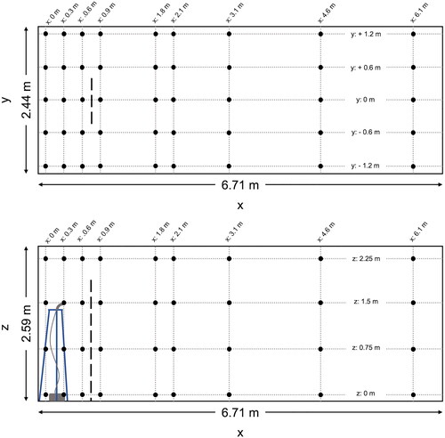
Each experiment was conducted with and without a barrier in place. The plastic barrier had dimensions 0.91 m × 1.83 m (W × H) and was located at x = 0.76 m, centered at y = 0 m, a distance of 0.46 m (1.5 ft) from the source. The barrier width and height above the source matched those determined to be most effective at reducing particle counts between the source and the receiver (Bartels et al. 2022). The bottom edge of the barrier rested on the floor, and it was suspended from the ceiling via fishing line to hold it in place.

Aerosolization

Fluorescent polystyrene latex (PSL) microspheres were aerosolized into the room for 20 min using a nebulizer (MisterNeb® Compressor Nebulizer System). They are easily viewed using microscopy, and the fluorescence differentiates the microspheres from background particles in the room. PSL microspheres of diameters 0.5 µm, 1 µm, 6.2 µm (referred to as 6 µm for the sake of brevity), 10.2 µm (10 µm), and 20.2 µm (20 µm) (Polysciences, Inc., PA, USA) were used to represent the range of particle sizes generated by respiratory activities.

For each experiment, 5 mL of a suspension containing a single size of microspheres was added to the nebulizer. The suspensions contained various dilutions of stock suspensions of microspheres in nanopure water: 0.05 mL of 0.5 µm microspheres plus 4.95 mL of water; 2.5 mL of 1 µm microspheres plus 2.5 mL of water; and 0.5 mL of 6, 10, or 20 µm microspheres plus 4.5 mL of water (Table 1). The number concentrations of stock suspensions varied by five orders of magnitude, depending on the microsphere size. These volumes of stock and dilution factors were selected to balance a desire to achieve the same final concentration against limitations related to cost and the size of the nebulizer cup. The aerodynamic diameters of the microspheres were confirmed by nebulizing them in a benchtop chamber and measuring their size distributions using an aerodynamic particle sizer (TSI 3321). The measured diameters agreed with their nominal diameters (see Figure S1). The relative humidity inside the chamber was ∼60%, higher than in the experimental room, so the microspheres would carry even less residual water during the experiments and their transport should be consistent with their nominal diameters.

Table 1. Length of experiment (including nebulizer run time), PSL concentration in tube received from manufacturer (Polysciences, Inc, PA, USA) and volume added to nebulizer (diluted to a final volume of 5 mL in nanopure water).

PSL microsphere diameter	Experiment duration, h (without barrier, with barrier)	PSL microsphere stock concentration (Ci), # mL^−1	Volume added to nebulizer (Volneb), mL	Final concentration in nebulizer, # mL^−1
0.5 µm	23.5, 23.1	3.64 × 10^11	0.05	3.64 x 10^9
1 µm	23.9, 24.0	4.55 x 10^10	2.5	2.28 x 10^10
6 µm	18.0, 21.3	2.10 x 10^8	0.5	2.10 x 10^7
10 µm	3.4, 3.2	4.55 x 10^7	0.5	4.55 x 10^6
20 µm	1.3, 1.5	5.68 x 10^6	0.5	5.68 x 10^5

The outlet of the nebulizer was placed on a tripod at x = 0.3 m, y = 0 m, z = 1.5 m (Figure 1). Tubing with an inner diameter of 0.5 cm and a gentle 90° bend was attached to the nebulizer cup to allow the cup to remain in an upright orientation while directing the output horizontally to match the direction of a jet generated by speech. The outlet speed was 4.7 m s⁻¹, in the range of normal speech for both males and females (Gupta, Lin, and Chen 2010). Compared to the number of particles released if a person says “aah” for 20 min (Morawska et al. 2009), the number of particles produced by the nebulizer was higher for the 0.5, 1, and 6 µm microspheres and comparable for the 10 and 20 µm microspheres. The nebulizer ran for 20 min at the start of each experiment before being turned off.

Indoor environmental conditions

The HVAC unit in the room was turned off for the duration of these experiments, and obvious sites of infiltration were sealed off using duct tape. The ACR in the room was calculated using the carbon dioxide (CO₂) decay method (Allen et al. 2020). Briefly, dry ice was introduced in the room to achieve a peak concentration of 2000–5000 ppm. A fan was used to promote mixing and was turned off after the peak CO₂ concentration was achieved. CO₂ mixing ratios were used to calculate the ACR in the room using the following equation: (1) $$\mathrm{A}\text{CR}=-\frac{1}{t_{\mathit{\text{end}}}-t_{\mathit{\text{start}}} }*\hspace{0.17em}\ln \left(\frac{C_{\mathit{\text{end}}} - C_{\mathit{\text{ambient}}}}{C_{\mathit{\text{start}}} -C_{\mathit{\text{ambient}}}}\right)$$(1) where C_end and C_start are the CO₂ mixing ratios recorded at the end and start of the CO₂ decay curve, respectively. C_ambient is the background CO₂ mixing ratio recorded in the room prior to the start of the experiment and t_end and t_start are the times associated with the end and start of the decay curve (hr). A logger (HOBO MX1102, Onset Computer Corporation, MA, USA) recorded CO₂ mixing ratios every 30 s. This was repeated three times.

During each experiment, the logger recorded temperature and relative humidity every 10 min (except for the 20 µm, no-barrier scenario in which measurements were collected every 1 min) (Figures S2–S6). The temperature in the room remained stable for the duration of all experiments, around 20–21 °C. The relative humidity exhibited greater variability; lower relative humidity values (< 20%) were usually associated with lower outdoor temperatures (< 9 °C) while higher relative humidity values (> 30%) were usually associated with either rain or warmer temperatures (> 9 °C). A mini fog machine with glycerol (MicroFogger 3 Lite, Vosentech, PA, USA) was used (not during experiments) to visualize airflow in the room, as a form of smoke test.

Sample collection

Glass microscope slides (25 × 75 mm) were placed on the sampling platforms prior to the beginning of each experiment and were retrieved at the end. Each experiment concluded when the vertical flux for the respective particle size was near zero, according to modeling calculations described below (∼24 h for 0.5 and 1 µm microspheres, ∼18 h for 6 µm microspheres, ∼4 h for 10 µm microspheres, and ∼1 h for 20 µm microspheres). At this time, each microscope slide was collected and placed in a petri dish that was sealed with Parafilm and stored at room temperature until analysis. All samples were collected with by a masked researcher.

Data collection

Slides were imaged using a fluorescence microscope (EVOS FL Auto Microscope and EVOS FL Auto Imaging Software, ThermoFisher, MA, USA). Different magnification levels were utilized to image the microspheres; the ‘GFP’ setting was used to view fluorescent microspheres at 20X, while the ‘Trans’ setting was used at 10× and 4× magnification levels. For each sample, 12 photos at randomly selected locations were captured to determine particle number per square centimeter. If there were no observed microspheres in those photos, 12 additional photos were captured at other randomly selected locations. This was repeated twice for a maximum of 36 photos. If no microspheres were observed in any photo but were observed during a quick scan of the sample, that sample was classified as ‘too few to count’ (TFTC). Results were expressed as the ratio of the number of particles at each sampling location, N, to the total number particles observed at all sampling locations per experiment, N_tot. Any microspheres observed on TFTC samples were excluded from the N_tot calculation. The TFTC threshold corresponded to a N/N_tot value of 2 × 10⁻⁴. Otherwise, the sample was classified as ‘not detectable’ (ND), and N/N_tot was set to 1 × 10⁻⁴. Table 2 lists values of N and N_tot for each experiment for the TFTC and ND thresholds.

Table 2. Total microsphere numbers observed (N_tot) and quantification limits for each microsphere size. Too few to count (TFTC) was set to N/N_tot = 2 × 10⁻⁴ and not detectable (ND) was set to N/N_tot = 1 × 10⁻⁴.

PSL microsphere diameter (µm)	Experimental setup	NTOT (no. of particles)	TFTC	ND
			N (no. of particles per sample)	N (no. of particles per sample)
0.5	No barrier	2.8 × 10^6	N/A	N/A
	Barrier	1.3 × 10^7
1	No barrier	5.6 × 10^7	N/A	N/A
	Barrier	8.6 × 10^6
6	No barrier	4.1 × 10^4	8.2	4.1
	Barrier	2.1 × 10^4	4.2	2.1
10	No barrier	2.7 × 10^3	< 1	< 1
	Barrier	0^a
20	No barrier	1.0 × 10^2	< 1	< 1
	Barrier	0^a

^a No microspheres were observed during the 10 and 20 µm barrier experiments; all samples were either TFTC or ND, therefore, N_tot could not be calculated.

N/A indicates that no samples were below the quantification limit and no samples were classified as TFTC or ND.

Large droplets that dripped out of the nebulizer outlet and that contained multiple microspheres were excluded from this analysis. The sampling location closest to the nebulizer outlet was excluded from analysis due to the large number of droplets on the slides that obscured counting of individual microspheres. Contour maps were generated using the plotly package and graphs were generated using the ggplot package in R (version 4.2.4). The plotly package interpolates data using the centripetal Catmull–Rom method. Contour maps are expressed as the ratio, N/N_tot.

Modeling

A mass-balance model was used to estimate the vertical flux of particles due to settling. The purpose of this calculation was to define the duration of each experiment. Table 3 lists all variables and their values. The settling velocity, V_t, was calculated as a function of the nominal size of the microspheres and was adjusted for slip correction. (2) $$\frac{\mathit{\text{dC}}}{\mathit{\text{dt}}}=\left[-\left(\frac{Q+V_{\mathit{\text{t }}}{A}_{\mathit{\text{floor}}}}{{\mathit{\text{Vol}}}_{\mathit{\text{room}}}}\right)*C\right]$$(2)

Table 3. List of variables used in modeling.

Variable name	Units	Description	Value
Vt	m s^−1	Settling velocity	$\frac{\mathrm{g}{\mathrm{ }*\mathrm{ }\mathrm{D}}_{\mathrm{p}}^2\mathrm{ }*\mathrm{ }\mathrm{(}{\mathrm{\rho }}_{\mathrm{p}}-\mathrm{ }{\mathrm{\rho }}_{\mathrm{f}}\mathrm{)}\mathrm{ }*\mathrm{ }{\mathrm{C}}_{\mathrm{c}}}{18\mathrm{ }*\mathrm{ }{\mathrm{\mu }}_{\mathrm{f}}}$
${\mathrm{C}}_{\overline{\mathrm{a}}}$	No. of particles m^−3	Assumed concentration of PSL microspheres aerosolized in room	$\frac{{\mathrm{C}}_{\mathrm{i}}\text{ * }{\text{Vol}}_{\text{neb}}}{{\text{Vol}}_{\text{room}}}$
Ci	No. of particles mL^−1	PSL microsphere stock concentration	See Table 1
Volneb	mL	Volume of PSLs added to nebulizer	See Table 1
Volroom	m^3	Volume of room	42.4
Q	m^3 s^−1	Volumetric flow rate	λ$\mathrm{*}\mathrm{ }$ Volroom
λ	s^−1	Air exchange rate	1.6 × 10^−4
Afloor	m^2	Area of floor	16.4
Aslide	m^2	Area of microscope slide	1.9 × 10^−3
t	s	Settling time	Independent variable^a
g	m s^−2	Acceleration due to gravity	9.81
Dp	m	PSL microsphere diameter	0.5, 1, 6.2, 10.2, 20.2 (× 10^−6)
ρp	kg m^−3	Density of PSL microspheres	1050
ρf	kg m^−3	Density of air in room	1.2
µf	kg m^−1 s^−1	Dynamic viscosity of air	1.85 × 10^−5
Cc		Slip correction coefficient (for Dp < 5 µm)	$1+\text{Kn}\mathrm{ }[1.257+0.4\mathrm{ }*\mathrm{ }\hspace{0.17em}\exp \hspace{0.17em}\left(\frac{-1.1}{\text{Kn}}\right)]$
Kn	–	Knudson number	$\frac{2\mathrm{ }*\mathrm{ }0.065}{{\mathrm{D}}_{\mathrm{p}}}$
Cavg	No. of particles m^−3	Average airborne concentration at each sampling location	Equation (5)(5) $$C_{\mathit{\text{avg}}}=\frac{N}{V_t t_e A_{\mathit{\text{slide}}}}$$(5)
N	No. of particles	Number of observed particles per microscope slide	Determined experimentally
te	s	Exposure time (time for 3 air changes or time to settle 1.5 m)	0.5 µm: 1.8 × 10^4 1 µm: 1.8 × 10^4 6 µm: 1.3 × 10^3 10 µm: 470 20 µm: 120

^aSettling time was the independent variable used in Equations (3)(3) $$C\left(t\right)=C_{\overline{a}} \hspace{0.17em}\exp \hspace{0.17em}\left[-\left(\frac{Q+V_{\mathit{\text{t }}}{A}_{\mathit{\text{floor}}}}{{\mathit{\text{Vol}}}_{\mathit{\text{room}}}}\right)*t\right]$$(3) and (4)(4) $$\text{Flux}=V_t\mathit{\text{ C}}=V_t{\mathit{\text{ C}}}_{\overline{a}} * \hspace{0.17em}\exp \hspace{0.17em}\left[-\left(\frac{Q + V_{\mathit{\text{t }}}{A}_{\mathit{\text{floor}}}}{{\mathit{\text{Vol}}}_{\mathit{\text{room}}}}\right)*t\right]$$(4) , and therefore different values were used when calculating flux.

Equation (3)(3) $$C\left(t\right)=C_{\overline{a}} \hspace{0.17em}\exp \hspace{0.17em}\left[-\left(\frac{Q+V_{\mathit{\text{t }}}{A}_{\mathit{\text{floor}}}}{{\mathit{\text{Vol}}}_{\mathit{\text{room}}}}\right)*t\right]$$(3) shows the solution for C(t): (3) $$C\left(t\right)=C_{\overline{a}} \hspace{0.17em}\exp \hspace{0.17em}\left[-\left(\frac{Q+V_{\mathit{\text{t }}}{A}_{\mathit{\text{floor}}}}{{\mathit{\text{Vol}}}_{\mathit{\text{room}}}}\right)*t\right]$$(3) where $C_{\overline{a}}$ is the initial concentration of microspheres in the room, assuming that all were nebulized and instantaneously dispersed throughout the room. Equation (4)(4) $$\text{Flux}=V_t\mathit{\text{ C}}=V_t{\mathit{\text{ C}}}_{\overline{a}} * \hspace{0.17em}\exp \hspace{0.17em}\left[-\left(\frac{Q + V_{\mathit{\text{t }}}{A}_{\mathit{\text{floor}}}}{{\mathit{\text{Vol}}}_{\mathit{\text{room}}}}\right)*t\right]$$(4) shows the instantaneous flux of particles: (4) $$\text{Flux}=V_t\mathit{\text{ C}}=V_t{\mathit{\text{ C}}}_{\overline{a}} * \hspace{0.17em}\exp \hspace{0.17em}\left[-\left(\frac{Q + V_{\mathit{\text{t }}}{A}_{\mathit{\text{floor}}}}{{\mathit{\text{Vol}}}_{\mathit{\text{room}}}}\right)*t\right]$$(4)

The time-averaged airborne concentration, C_avg, found at a particular sampling location over the duration of each experiment was estimated based on the observed number of microspheres at each location: (5) $$C_{\mathit{\text{avg}}}=\frac{N}{V_t t_e A_{\mathit{\text{slide}}}}$$(5) where N is the number of microspheres observed at a sampling location and t_e is the exposure time, defined as either the time required for three air changes in the room (∼5 h) or the time for a microsphere to settle 1.5 m, whichever is smaller. All calculations were conducted in Microsoft Excel.

Results

Twelve experiments were conducted: with and without the barrier for each of 0.5, 1, 6, 10, and 20 µm microspheres and a set of replicates for the 1 µm microspheres. The ACR of the room was 0.6 ± 0.2 h⁻¹. Results are reported as contour maps displaying the distribution of particles in the room in terms of the ratio of the number of observed microspheres at each sampling location, N, to the total number of microspheres observed for the entire experiment, N_tot. Any samples that were classified as TFTC (where microspheres were observed, but not quantified) were excluded from the calculation of N_tot. Time-averaged airborne concentrations of microspheres at each sampling location, estimated by Equation (5)(5) $$C_{\mathit{\text{avg}}}=\frac{N}{V_t t_e A_{\mathit{\text{slide}}}}$$(5) , are also discussed. Ideally, experiments conducted with and without the barrier would have been similar enough to allow direct comparison of the results and to estimate the intake fraction at various locations. After completing the experiments, we determined that there was sufficient variability in the ACR and fate of microspheres in large droplets between experiments that a more quantitative analysis would have been highly uncertain. Thus, our analysis focuses on differences in the spatial distribution of microspheres between experiments.

A mini fog machine was used to visualize the movement of air in the room both with and without the barrier. Although the HVAC system in the room was turned off and obvious sites of infiltration were sealed, air movement was still observed. Without the barrier in place, particles that were released at the source moved upwards toward the ceiling and followed the length of the ceiling in the x-direction while also dispersing laterally in the y-direction. This upward movement was exaggerated with the barrier in place (see Video SI). This transport was at least partly due to the momentum of the jet exiting the fog machine. Observation of particles released at other locations in the room indicated no dominant air flow pattern in the room, except near the doors, where there was some advection along the walls either toward or away from the doors. With the barrier in place, we observed accumulation of particles between the barrier and nebulizer. At other locations on the opposite side of the barrier and >1 m away from it, the air flow patterns appeared similar as in the case without the barrier.

 0.5 μm microspheres

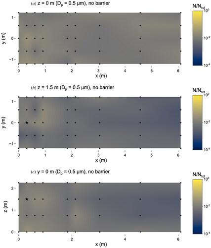
In the absence of a barrier, 0.5 µm microspheres were evenly distributed throughout the room. The highest number of microspheres was observed at x = 0.3 m, y = 0 m, z = 0 m, which is located on the floor below the nebulizer source (Figure 2). At this location, N/N_tot = 0.03 (i.e., 3 percent of the total number of particles observed), and the corresponding time-averaged airborne concentration was 2.3 × 10² particles cm⁻³. The minimum number of microspheres was found at x = 6.1 m, y = 0.6 m, z = 1.5 m, the most distant x-location from the nebulizer source. At this location, N/N_tot = 0.001, corresponding to a concentration of 1.1 × 10¹ particles cm⁻³. Overall, the number of microspheres at different sampling locations throughout the room varied by about one order of magnitude. The total number of microspheres quantified during all experiments is listed in Table 2.

Figure 2. Distribution of 0.5 µm microspheres in the room with no barrier in place. (a) x–y plane at z = 0 m level; (b) x–y plane at z = 1.5 m level; and (c) x–z plane at y = 0 m level. Closed dots represent sampling points and star represents location of nebulizer outlet. N represents the total observed microspheres settled on each 25 × 75 mm microscope slide and N_tot represents the total microspheres observed on all slides during this experiment.

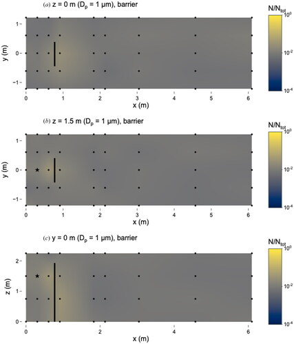
With the barrier at x = 0.76 m, the highest number of 0.5 µm microspheres was observed at the sampling location x = 0.6 m, y = 0 m, z = 1.5 m, which is 0.3 m in front of the nebulizer outlet (Figure 3). The ratio at this location, N/N_tot = 0.08, corresponds to a concentration of 3.2 x 10³ particles cm⁻³. The number of microspheres observed at different sampling locations varied by almost three orders of magnitude during this experiment, as the minimum number of observed microspheres occurred at two locations: x = 3.0 m, y = 1.2 m, z = 1.5 m and x = 6.1 m, y = 1.2 m, z = 1.5 m, where N/N_tot = 2.8 × 10⁻⁴ and the concentration was 1.1 × 10¹ particles cm⁻³.

Figure 3. Distribution of 0.5 µm microspheres in the room with barrier in place. (a) x–y plane at z = 0 m level; (b) x–y plane at z = 1.5 m level; and (c) x–z plane at y = 0 m level. Closed dots represent sampling points and star represents location of nebulizer outlet. Solid line at x = 0.76 m represents location of barrier. N represents the total observed microspheres settled on each 25 × 75 mm microscope slide and N_tot represents the total microspheres observed on all slides during this experiment.

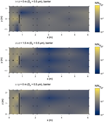
To gain a better understanding of the impact of the barrier on the spatial distribution of microspheres in the immediate vicinity of the barrier, we compared the number of microspheres at locations around the barrier (at breathing height, z = 1.5 m) to the number at a reference location (x = 0.9 m, y = 0 m, z = 1.5 m) (Figure S7). This reference location represents a “receiver” who is standing directly in front of a “source” person, with the barrier between the two. Relative to the receiver, the number of microspheres was higher in almost all locations at z = 1.5 m (i.e. breathing height) between x = 0 m and x = 1.8 m with the barrier in place. This indicates that the receiver would have the lowest exposure to 0.5 µm particles relative to other individuals located on the same side of the barrier as the source or around the sides of the barrier (y = ±0.6 and ±1.2 m). Without the barrier, exposures at all x-locations ≤1.8 m from the nebulizer were similar to the receiver’s.

The effect of the barrier was more pronounced for the 0.5 µm microspheres compared to those of other sizes. In general, microspheres were observed in higher numbers, by about a factor of 50, on the source-side of the barrier compared to the opposite side. This accumulation was most pronounced at z = 1.5 m and y = 0 m (Figures 3b and c). At all sampling locations except for one (x = 0.6 m, y = −1.2 m, z = 0 m) on the source-side of the barrier, the fraction of microspheres was either higher or not substantially different with the barrier compared to without it (ratios for z = 1.5 m shown in Figure S8). The fraction of deposited microspheres at breathing height was lower on the opposite side of the barrier at x = 0.9 m, y = 0 m, z = 1.5 m compared to the source-side at x = 0.6 m, y = 0 m, z = 1.5 m. This suggests that the barrier may be effective at reducing exposure to respiratory emissions of 0.5 µm particles at the location on the opposite side of the barrier (the receiver location, x = 0.9 m, y = 0 m, z = 1.5 m) relative to the source, compared to the scenario with no barrier.

 1 μm microspheres

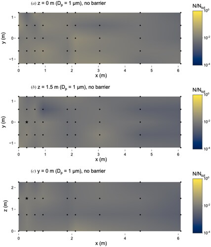
In the absence of the barrier, the 1 µm microspheres were evenly distributed throughout the room; the number of microspheres deposited at different locations varied by about one order of magnitude (Figure 4). The maximum number of microspheres was observed at x = 0 m, y = 0.6 m, z = 0 m, where N/N_tot = 0.02 and the concentration was 1.1 × 10³ particles cm⁻³. The minimum number of microspheres was observed at x = 0.9 m, y = 0.6 m, z = 1.5 m, where N/N_tot = 0.002 and the concentration was 9.0 × 10¹ particles cm⁻³. There was no noticeable reduction in the number of 1 µm microspheres at the furthest distances (e.g. x = 3.0, 4.6 or 6.1 m) from the source.

Figure 4. Distribution of 1 µm microspheres in the room with no barrier in place. (a) x–y plane at z = 0 m level; (b) x–y plane at z = 1.5 m level; and (c) x–z plane at y = 0 m level. Closed dots represent sampling points and star represents location of nebulizer outlet. N represents the total observed microspheres settled on each 25 × 75 mm microscope slide and N_tot represents the total microspheres observed on all slides during this experiment.

With the barrier, the number of microspheres observed at different sampling locations still only varied by about one order of magnitude (Figure 5). The maximum number of microspheres was observed 0.3 m in front of the source (x = 0.6 m, y = 0 m, z = 1.5 m). At this location, N/N_tot = 0.03 and the concentration was 2.3 × 10² particles cm⁻³. Two locations had the minimum number: x = 0 m, y = −0.6 m, z = 1.5 m (behind the source) and x = 2.1 m, y = −0.6 m, y = 0 m. At these locations, N/N_tot = 0.006 and the corresponding concentration was 4.2 × 10¹ particles cm⁻³.

Figure 5. Distribution of 1 µm microspheres in the room with barrier in place. (a) x–y plane at z = 0 m level; (b) x–y plane at z = 1.5 m level; and (c) x–z plane at y = 0 m level. Closed dots represent sampling points and star represents location of nebulizer outlet. Solid line at x = 0.76 m represents location of barrier. N represents the total observed microspheres settled on each 25 × 75 mm microscope slide and N_tot represents the total microspheres observed on all slides during this experiment.

Compared to the number of 1 µm microspheres at the receiver location (x = 0.9 m, y = 0 m, z = 1.5 m), most sampling locations around the barrier at z = 1.5 m either had fewer 1 µm microspheres than the receiver location or not a substantially different number (Figure S7). Comparing the 1 µm to the 0.5 µm microspheres, the relative ratios of the receiver location to other locations at z = 1.5 m were lower for the 1 µm particles, indicating that exposure to 1 µm microspheres would be lower at most locations at breathing height around the barrier than exposure to 0.5 µm microspheres.

The barrier had a less noticeable effect for the 1 µm microspheres than the 0.5 µm microspheres. At breathing height (z = 1.5 m), there was about a 50% decrease in the number of microspheres observed on the side of the barrier opposite the source (x = 0.9 m, y = 0 m) than on the side with the source (x = 0.6 m, y = 0 m). However, the addition of the barrier did not result in a major difference at 89% (95/107) of sampling locations. The barrier led to reductions in microsphere number at locations found at x-distances of 2.1 m and 3.0 m (data not shown). Two locations on the opposite side of the barrier from the source had increases in microsphere numbers (x = 0.9 m, y = 0 m, z = 0 m and 0.75 m); for these locations, the barrier had the opposite impact on the 1 µm microspheres as compared to the 0.5 µm microspheres.

 6 μm microspheres

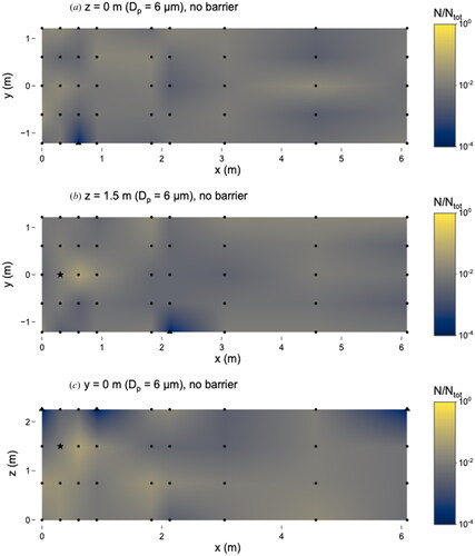
The 6 µm microspheres were observed at most locations (102/107) without the barrier in place, and 5/107 locations were categorized as TFTC. The particles were detected at every x-distance within the room, indicating that 6 µm particles can travel distances of at least 5.8 m (Figure 6). The maximum number of 6 µm microspheres was observed at x = 0.6 m, y = 0 m, z = 1.5 m, at the location in front of the nebulizer source, where the corresponding concentration was 8.4 × 10⁻¹ particles cm⁻³ and N/N_tot = 0.06. There were five locations where the 6 µm microspheres were categorized as TFTC, corresponding to N/N_tot = 2 × 10⁻⁴.

Figure 6. Distribution of 6 µm microspheres in the room with no barrier in place. (a) x–y plane at z = 0 m level; (b) x–y plane at z = 1.5 m level; and (c) x–z plane at y = 0 m level. Closed dots represent sampling points, the star represents location of nebulizer outlet, and triangles represent sampling locations that were classified as “too few to count”. N represents the total observed microspheres settled on each 25 × 75 mm microscope slide and N_tot represents the total microspheres observed on all slides during this experiment.

With the barrier, 6 µm microspheres were observed at 79/107 locations, while 28/107 were TFTC (N/N_tot = 2 × 10⁻⁴) (Figure 7). The maximum number of microspheres was observed at the same location as the no-barrier scenario (x = 0.6 m, y = 0 m, z = 1.5 m) where N/N_tot = 0.07 the concentration was 5.3 × 10⁻¹ particles cm⁻³. The barrier did not prevent 6 µm microspheres from traveling long distances, as they were detected at x = 6.1 m, although more sampling locations were categorized as TFTC than in the no-barrier scenario. In both scenarios, the number of microspheres observed on slides varied by about 2.5 orders of magnitude.

Figure 7. Distribution of 6 µm microspheres in the room with barrier in place. (a) x–y plane at z = 0 m level; (b) x–y plane at z = 1.5 m level; and (c) x–z plane at y = 0 m level. Closed dots represent sampling points, the star represents location of nebulizer outlet, and triangles represent sampling locations that were classified as “too few to count”. Solid line at x = 0.76 m represents location of barrier. N represents the total observed microspheres settled on each 25 × 75 mm microscope slide and N_tot represents the total microspheres observed on all slides during this experiment.

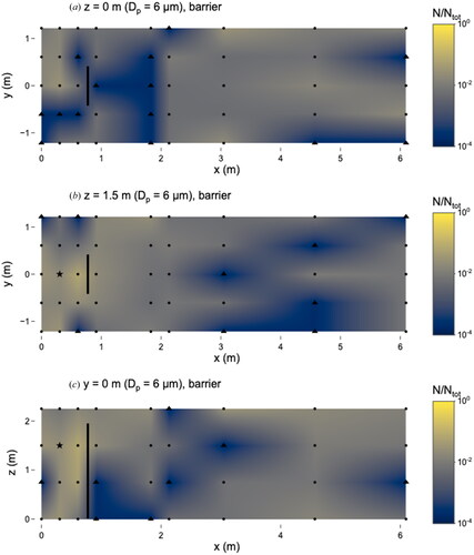
There were no differences between any sampling locations when comparing the scenarios with and without the barrier; this is due in part to the low total number of observed microspheres (compared to the 0.5 and 1 µm experiments) (Table 2). Our results suggest that personal exposure to 6 µm particles can be highly variable depending on the location relative to the barrier.

Relative to the receiver location (x = 0.9 m, y = 0 m, z = 1.5 m), most locations at breathing height either had a smaller proportion of microspheres or were not different from the receiver location when the barrier was present, which indicates that an individual at that location may not experience a lower exposure to 6 µm particles compared to other locations at breathing height around the barrier.

 10 μm and 20 μm microspheres

Particles of 10 µm were only observed in the immediate vicinity surrounding the nebulizer outlet in the experiment without a barrier (Figure 8). Most locations were categorized as ‘not detectable’ except for x = 0.9 m, y = 0.6 m, z = 0 m, which was categorized as TFTC. The addition of the barrier (Figure 9) resulted in no differences in the number of 10 µm particles observed, due in part to the low particle counts; all locations where microspheres were observed were categorized as TFTC. A similar pattern was observed for the 20 µm particles (Figures 10 and 11).

Figure 8. Distribution of 10 µm microspheres in the room with no barrier in place. (a) x–y plane at z = 0 m level; (b) x–y plane at z = 1.5 m level; and (c) x–z plane at y = 0 m level. Closed dots represent sampling points, star represents location of nebulizer outlet, triangles represent sampling locations classified as “too few to count” and x’s represent those that were classified as “not detectable”. N represents the total observed microspheres settled on each 25 × 75 mm microscope slide and N_tot represents the total microspheres observed on all slides during this experiment.

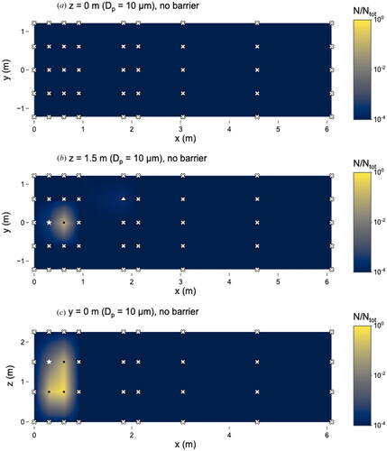
Figure 9. Distribution of 10 µm microspheres in the room with barrier in place. (a) x–y plane at z = 0 m level; (b) x–y plane at z = 1.5 m level; and (c) x–z plane at y = 0 m level. Closed dots represent sampling points, star represents location of nebulizer outlet, triangles represent sampling locations classified as “too few to count” and x’s represent those classified as “not detectable”. Solid line at x = 0.76 m represents location of barrier. N represents the total observed microspheres settled on each 25 × 75 mm microscope slide and N_tot represents the total microspheres observed on all slides during this experiment.

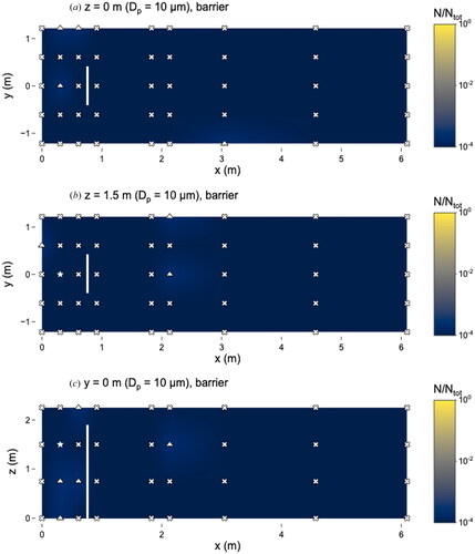
Figure 10. Distribution of 20 µm microspheres in the room with no barrier in place. (a) x–y plane at z = 0 m level; (b) x–y plane at z = 1.5 m level; and (c) x–z plane at y = 0 m level. Closed dots represent sampling points, star represents location of nebulizer outlet, triangles represent sampling locations classified as “too few to count” and x’s represent those classified as “not detectable”. N represents the total observed microspheres settled on each 25 × 75 mm microscope slide and N_tot represents the total microspheres observed on all slides during this experiment.

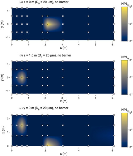
Figure 11. Distribution of 20 µm microspheres in the room with barrier in place. (a) x–y plane at z = 0 m level; (b) x–y plane at z = 1.5 m level; and (c) x–z plane at y = 0 m level. Closed dots represent sampling points, star represents location of nebulizer outlet, triangles represent sampling locations classified as “too few to count” and x’s represent those classified as “not detectable”. Solid line at x = 0.76 m represents location of barrier. N represents the total observed microspheres settled on each 25 × 75 mm microscope slide and N_tot represents the total microspheres observed on all slides during this experiment.

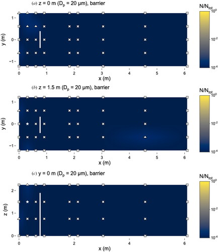
Although the 10 and 20 µm microspheres were observed in low numbers, particles of these sizes were still capable of traveling long distances. Even with the barrier present, 10 µm microspheres were observed at x = 3.1 m (Figure 9a). Microspheres of 20 µm were observed at x = 6.1 m without the barrier (Figure 10c) and x = 4.6 m with the barrier (Figure 11b).

Discussion

The barrier resulted in altered patterns of transport and deposition of particles in the room. These differences varied by particle size and were particularly notable for the 0.5 and 6 µm microspheres. These microspheres accumulated on the source-side of the barrier, both along the centerline (y = 0 m) and laterally (y = ±1.2 and ±0.6 m). For the 0.5 µm microspheres, values of N/N_tot either increased or did not change. As the 1 µm microspheres were intermediate in size between the 0.5 µm and 6 µm ones, one would expect to observe differences with vs. without the barrier, but it did not appear to impact the 1 µm microspheres to the same extent, even upon repetition of the experiments with 1 µm microspheres (Figures S9 and S10). Most larger microspheres (10 and 20 µm) did not travel far enough to reach the barrier; however, a small fraction of them could travel x-distances of 3.1 m (10 µm) and 4.6 m (20 µm), even with the barrier present. This indicates that particles of these sizes can be carried some distance by air currents within the room and are not subject to immediate gravitational settling to the floor.

In all experiments with 0.5, 1, and 6 µm microspheres (with and without the barrier), there was no apparent decrease in particle numbers at x-locations further away from the source (x > 2.1 m) compared to many of the locations within six feet of the source (x ≤ 2.1 m). This indicates that over periods of 1 h or more, the “six-foot rule” is not sufficient for protection from particles of these sizes, even when using a barrier. Our findings in the experiments without a barrier for 0.5, 1, and 6 µm microspheres support investigations of outbreaks showing that SARS-CoV-2 transmission can occur in enclosed environments with poor ventilation, even when individuals are more than six feet apart (Charlotte 2020; Lu et al. 2020; Katelaris et al. 2021; Li et al. 2021). OSHA guidelines for fixed workstations when workers are unable to remain six feet apart recommend the use of barriers to prevent face-to-face transmission (Occupational Safety and Health Administration 2021). Under the conditions of this study, microspheres up to 6 µm could travel up to 5.8 m from the source with the barrier present, emphasizing the need for other protective measures. Our findings highlight the importance of the need for proper ventilation or other protective measures to prevent transmission of respiratory emissions, as six feet is not a sufficient distance over long time scales, even with a barrier.

These results are not surprising given air flow velocities that have been measured in indoor workplaces (Baldwin and Maynard, 1998) and domestic environments (Matthews et al. 1989). According to CFD modeling in a classroom without ventilation, the air flow velocity was approximately 0.1 m s⁻¹, and with no barriers in place, gaseous pollutants could potentially travel up to 9 m from the source (Ren et al., 2021). At a horizontal velocity of 0.1 m s⁻¹, a 6 µm particle could travel 125 m in the horizontal direction before settling to the ground from a height of 1.5 m. Foster and Kinzel (2021a) found that in a classroom with no ventilation and no filtration (and no physical barriers), the highest infection probabilities occurred at 4.5 m (15 ft) and concluded that risk was not associated with distance because peak infections were observed outside physical distancing guidelines. These studies agree with our findings that particles up to 6 µm could be transported throughout the room (up to 5.8 m away from the source), even without mechanical ventilation.

Other studies that have evaluated the impact of the barriers experimentally and through CFD modeling have highlighted the importance of ventilation in reducing transmission. Foster and Kinzel (2021b) concluded that there was no difference in SARS-CoV-2 transmission when modeling the impact of desk shields compared to no mitigation strategy in a classroom where no fresh air was introduced. In another CFD study, the implementation of barriers in a classroom reduced the total particles deposited onto students, but 2.4 m was an inadequate distance to eliminate SARS-CoV-2 transmission. In that same study, the students’ transmission risk was dependent on their location relative to the air conditioning units (Abuhegazy et al. 2020). CFD modeling showed that fully-extended hospital curtains, serving as physical barriers, reduced peak concentrations for neighboring patients in a ventilated hospital room (Ching et al. 2008).

Bartels et al. (2022) employed a similar experimental layout as in our study in terms of barrier placement relative to a source and receiver with measurements of different sized-particles. With the same barrier dimensions, we observed a 98% efficiency in blocking airborne particles (calculated using Bartels’ Equation 1) for small sizes (∼0.5 µm), compared to their 84%, indicating that the barrier is effective at protecting susceptible individuals from small particles. However, we observed efficiencies of 57% and −19% for 1 µm and 6 µm particles, respectively, compared to 81% efficiency for both sizes as reported by Bartels et al. These discrepancies could be due to differences in ventilation rates (2 h⁻¹ in Bartels et al. vs. 0.6 h⁻¹ in our study), source strength (two simulated coughs vs. 20 min of continuous talking), sample integration time (10 min vs. 1–24 h), or sampling approach (continuous active sampling with two optical particle counters vs. passive sampling).

Zhang et al. (2022) evaluated the impact of a barrier on transmission using CO₂ to simulate exhaled particles and concluded that at short distances (<0.8 m) between manikins, the barrier successfully created two ‘micro environments’. Contaminants became trapped in a stagnant zone near the source, and the target (receiver) manikin had low exposure indexes, indicating good air quality near the receiver. The receiver manikin served as an active sampler with a flow rate of 9.32 L min⁻¹ to represent inhalation. Our findings provide a more complete representation of the ‘microenvironments’ surrounding a source and receiver and demonstrate that exposure is dependent on particle size in the presence of a barrier. Zhang et al. (2022) also concluded that the ventilation pattern in the room impacted the receiver’s exposure.

Li et al. (2022) investigated different layouts of a barrier between a seated source and receiver. With the source and receiver face-to-face and 1.5 m apart (the source is 0.6 m from the barrier), the receiver’s exposure to 0.25–2.5 µm particles was reduced by 99%. We did not observe a similar reduction in exposure at that approximate location relative to the barrier for 0.5 and 1 µm microspheres, likely due to the differences in ventilation rates (4.18 h⁻¹ with mixing ventilation in Li et al. vs. 0.6 h⁻¹ in our study). Another difference is the use of a particle counter at a flow rate of 1.2 L min⁻¹ in Li et al., whereas we employed passive samplers. When the source and receiver were both seated on the same side of the barrier (1.1 m apart), the particles in the coughing jet lost horizontal momentum due to the barrier, resulting in an increased number of particles at the receiver’s inhalation zone. We observed a similar phenomenon in our study, with relatively greater numbers of 0.5 µm microspheres observed on the same side of the barrier as the source, compared to the no-barrier scenario (Figure 3).

Cadnum, Jencson, and Donskey (2021) evaluated the impact of various barrier configurations (barriers of various sizes and barriers with and without openings) on bacteriophage MS2 concentrations. The authors concluded that a three-sided barrier (no opening) was effective at reducing MS2 plaque-forming units by about 50% when the manikin was 0.91 m from the nebulizer (and 0.61 m from the barrier). Differences between the study and ours include ventilation rate (6 h⁻¹ in Cadnum et al. vs. 0.6 h⁻¹ in our study), barrier type (three-sided vs. one-sided), sampling locations (tabletop and manikin vs. throughout the room), and sampling type (swab vs. passive particle deposition).

Physical barriers are likely to be helpful for mitigating the risk of transmission by aerosols during brief interactions between two people by temporarily corralling emitted respiratory particles on one side of the barrier, but our results indicate that barriers do not mitigate the overall risk of transmission over longer exposure times (>1 h). In fact, barriers may result in higher exposure to people on the same side of the barrier as the infected person, as with coworkers side-by-side behind a series of barriers along a counter or customers congregating on the opposite side. A person’s location relative to the barrier should also be considered, as exposure to particles <6 µm did not change at distances up to 5.8 m from the barrier. Barriers may also interfere with proper ventilation and removal of aerosols. For example, barriers were identified as a risk factor in a Covid-19 outbreak in a school office because they impeded air flow (Doron et al. 2021).

Our results indicate that in rooms with low ventilation rates, barriers may not be adequate protection for individuals within the room, as particles have the opportunity to travel around the barrier. When the ventilation rate cannot be increased, other control methods can provide individual protection. For example, required vs. optional masking was associated with a lower relative risk of Covid-19 incidence compared to desk barriers in schools in Georgia (Gettings et al. 2021). Additionally, daily symptom screening resulted in a lower odds ratio for Covid-19-related outcomes (Lessler et al. 2021). Zhang et al. (2022) evaluated the impact of personal protective equipment on source control, concluding that open face shields and mouth visors were more effective at short distances (<0.5 m) than closed face shields and surgical masks under displacement ventilation, but the authors did not study exposure to the receiver. In addition to universal masking as a control method, portable air cleaners are cost-effective and can provide protection against aerosols when the ventilation rate cannot be increased. Lindsley et al. (2021) found that portable HEPA air cleaners in a conference room reduced exposure by up to 65%, masks reduced exposure by 72% and the combination of air cleaners and masks reduced exposure by up to 90%. Dal Porto et al. (2022) characterized the performance of a Corsi-Rosenthal air cleaner (five MERV-13 filters mounted to a box fan) and observed significant decreases in airborne particle concentrations compared to commercial HEPA-based air cleaners when employed in a home office and classroom.

Although there were several limitations with this study design, the results improve our understanding of particle movement in a room with a barrier and can inform future experiments. This study considered a single size of barrier, rather than multiple sizes and configurations; simulated talking for 20 min, rather than breathing, coughing, or sneezing; and took place in a single room whose airflow patterns were particular to that room. Our study did not consider the impact of humans who would affect air flow patterns through their movement, thermal plumes, and exhalations (Nazaroff 2022). The trajectories of respiratory particles would be affected by the difference in temperature between exhaled and ambient air. Due to buoyancy, the particles might more easily be transported over the top of the barrier. The air-change rate (ACR) in the room varied by a factor of 2 and we were unable to measure the ACR during experiments. For this reason, results were expressed as a ratio to the total number of microspheres observed per experiment (as opposed to a fraction of total microspheres nebulized); results in absolute terms could not be compared across experiments. We did not measure the surface charge of the fluorescent polystyrene particles or the glass microscope slides; it is possible that particles could have been attracted to the glass surface. The loss of microspheres in large droplets (excluded in our analysis) is a source of uncertainty. Finally, our samples were time-integrated and do not represent exposures at short time scales.

Conclusions

This study adds to our knowledge about the impact of physical barriers on the spatial distribution of simulated respiratory particles in a poorly ventilated room. At breathing height (z = 1.5 m), the barrier was effective at reducing exposure of a receiver on the opposite side of the barrier from the source for 0.5 µm microspheres; however, individuals at certain other locations would experience higher exposure to 0.5 µm particles. The impact of the barrier depends on the size of particles. Particles smaller than 6 µm were generally well-mixed in the room and were able to travel up to 5.8 m away from the source, even with the barrier. Most larger particles (10 and 20 µm) did not travel as far, but some of them reached distances of 3.1 m or more. These results imply that barriers alone may not serve as adequate protection to others in the room, depending on their location relative to the barrier and the timescale of exposure.

Acknowledgments

We thank M. Storme Spencer, AJ Prussin II, Elizabeth Lawhon, and Virginia Tech Facilities for their assistance.

Additional information

Funding

The funding for this research was provided by the National Science Foundation under CBET-2029911.

References

- Abuhegazy, M., K. Talaat, O. Anderoglu, and S. V. Poroseva. 2020. Numerical investigation of aerosol transport in a classroom with relevance to COVID-19. Phys. Fluids 32 (10):103311. doi:10.1063/5.0029118.
- Allen, J., J. Spengler, E. Jones, and J. Cedeno-Laurent. 2020. 5-step guide to checking ventilation rates in classrooms.
- Asadi, S., A. S. Wexler, C. D. Cappa, S. Barreda, N. M. Bouvier, and W. D. Ristenpart. 2019. Aerosol emission and superemission during human speech increase with voice loudness. Sci. Rep. 9 (1):2348. doi:10.1038/s41598-019-38808-z.
- Bagherirad, M., P. Trevan, M. Globan, E. Tay, N. Stephens, and E. Athan. 2014. Transmission of tuberculosis infection in a commercial office. Med. J. Aust. 200 (3):177–179. doi:10.5694/mja12.11750.
- Baldwin, P., and A. Maynard. 1998. A survey of wind speeds in indoor workplaces. Ann. Occup. Hyg. 42 (5):303–313. doi:10.1016/S0003-4878(98)00031-3.
- Bartels, J., C. F. Estill, I.-C. Chen, and D. Neu. 2022. Laboratory study of physical barrier efficiency for worker protection against SARS-CoV-2 while standing or sitting. Aerosol Sci. Technol. 56 (3):295–303. doi:10.1080/02786826.2021.2020210.
- Cadnum, J. L., A. L. Jencson, and C. J. Donskey. 2021. Do plexiglass barriers reduce the risk for transmission of severe acute respiratory syndrome coronavirus 2 (SARS-CoV-2)? Infect. Control Hosp. Epidemiol. doi:10.1017/ice.2021.383.
- Centers for Disease Control and Prevention. 2021. Scientific brief: SARS-CoV-2 transmission. Accessed July, 2022. https://www.cdc.gov/coronavirus/2019-ncov/science/science-briefs/sars-cov-2-transmission.html.
- Charlotte, N. 2020. High rate of SARS-CoV-2 transmission due to choir practice in France at the beginning of the COVID-19 pandemic. J. Voice. 10.1016/j.jvoice.2020.11.029.
- Chia, P. Y., K. K. Coleman, Y. K. Tan, S. W. X. Ong, M. Gum, S. K. Lau, X. F. Lim, A. S. Lim, S. Sutjipto, P. H. Lee, et al. 2020. Detection of air and surface contamination by SARS-CoV-2 in hospital rooms of infected patients. Nat. Commun. 11 (1):2800. doi:10.1038/s41467-020-16670-2.
- Ching, W.-H., M. K. H. Leung, D. Y. C. Leung, Y. Li, and P. L. Yuen. 2008. Reducing risk of airborne transmitted infection in hospitals by use of hospital curtains. Indoor Built Environ. 17 (3):252–259. doi:10.1177/1420326X08091957.
- Cortellessa, G., L. Stabile, F. Arpino, D. E. Faleiros, W. van den Bos, L. Morawska, and G. Buonanno. 2021. Close proximity risk assessment for SARS-CoV-2 infection. Sci. Total Environ. 794:148749. doi:10.1016/j.scitotenv.2021.148749.
- Dal Porto, R., M. N. Kunz, T. Pistochini, R. L. Corsi, and C. D. Cappa. 2022. Characterizing the performance of a do-it-yourself (DIY) box fan air filter. Aerosol Sci. Technol. 56 (6):564–572. doi:10.1080/02786826.2022.2054674.
- Doron, S., R. R. Ingalls, A. Beauchamp, J. S. Boehm, H. W. Boucher, L. H. Chow, L. Corridan, K. Goehringer, D. Golenbock, L. Larsen, et al. 2021. Weekly SARS-CoV-2 screening of asymptomatic kindergarten to grade 12 students and staff helps inform strategies for safer in-person learning. Cell Reports Medicine 2 (11):100452. doi:10.1016/j.xcrm.2021.100452.
- Foster, A., and M. Kinzel. 2021a. Estimating COVID-19 exposure in a classroom setting: A comparison between mathematical and numerical models. Phys Fluids (1994) 33 (2):021904. doi:10.1063/5.0040755.
- Foster, A., and M. Kinzel. 2021b. SARS-CoV-2 transmission in classroom settings: Effects of mitigation, age, and Delta variant. Phys Fluids (1994) 33 (11):113311. doi:10.1063/5.0067798.
- Gettings, J., M. Czarnik, E. Morris, E. Haller, A. M. Thompson-Paul, C. Rasberry, T. M. Lanzieri, J. Smith-Grant, T. M. Aholou, E. Thomas, et al. 2021. Mask use and ventilation improvements to reduce COVID-19 incidence in elementary schools—Georgia, November 16–December 11, 2020. MMWR. Morb. Mortal. Wkly. Rep. 70 (21):779–784. doi:10.15585/mmwr.mm7021e1.
- Gilkeson, C. A., M. A. Camargo-Valero, L. E. Pickin, and C. J. Noakes. 2013. Measurement of ventilation and airborne infection risk in large naturally ventilated hospital wards. Build. Environ. 65:35–48. doi:10.1016/j.buildenv.2013.03.006.
- Gupta, J. K., C.-H. Lin, and Q. Chen. 2010. Characterizing exhaled airflow from breathing and talking. Indoor Air. 20 (1):31–39. doi:10.1111/j.1600-0668.2009.00623.x.
- Katelaris, A. L., J. Wells, P. Clark, S. Norton, R. Rockett, A. Arnott, V. Sintchenko, S. Corbett, and S. K. Bag. 2021. Epidemiologic evidence for airborne transmission of SARS-CoV-2 during church singing, Australia, 2020. Emerg. Infect. Dis. 27 (6):1677–1680. doi:10.3201/eid2706.210465.
- Lee, J., D. Yoo, S. Ryu, S. Ham, K. Lee, M. Yeo, K. Min, and C. Yoon. 2019. Quantity, size distribution, and characteristics of cough-generated aerosol produced by patients with an upper respiratory tract infection. Aerosol Air Qual. Res. 19 (4):840–853. doi:10.4209/aaqr.2018.01.0031.
- Lessler, J., M. K. Grabowski, K. H. Grantz, E. Badillo-Goicoechea, C. J. E. Metcalf, C. Lupton-Smith, A. S. Azman, and E. A. Stuart. 2021. Household COVID-19 risk and in-person schooling. Science 372 (6546):1092–7. doi:10.1126/science.abh2939.
- Li, W., A. Chong, B. Lasternas, T. G. Peck, and K. W. Tham. 2022. Quantifying the effectiveness of desk dividers in reducing droplet and airborne virus transmission. Indoor Air 32 (1):e12950. doi:10.1111/ina.12950.
- Li, X., J. Niu, and N. Gao. 2012. Characteristics of physical blocking on co-occupant’s exposure to respiratory droplet residuals. J. Cent. South Univ. 19 (3):645–650. doi:10.1007/s11771-012-1051-0.
- Li, Y. 2021. Hypothesis: SARS‐CoV‐2 transmission is predominated by the short‐range airborne route and exacerbated by poor ventilation. Indoor Air. 31 (4):921–925. doi:10.1111/ina.12837.
- Li, Y., H. Qian, J. Hang, X. Chen, P. Cheng, H. Ling, S. Wang, P. Liang, J. Li, S. Xiao, et al. 2021. Probable airborne transmission of SARS-CoV-2 in a poorly ventilated restaurant. Build. Environ. 196:107788. doi:10.1016/j.buildenv.2021.107788.
- Lindsley, W. G., R. C. Derk, J. P. Coyle, S. B. Martin, K. R. Mead, F. M. Blachere, D. H. Beezhold, J. T. Brooks, T. Boots, and J. D. Noti. 2021. Efficacy of portable air cleaners and masking for reducing indoor exposure to simulated exhaled SARS-CoV-2 aerosols—United States, 2021. MMWR. Morb. Mortal. Wkly. Rep. 70 (27):972–976. doi:10.15585/mmwr.mm7027e1.
- Lindsley, W. G., T. A. Pearce, J. B. Hudnall, K. A. Davis, S. M. Davis, M. A. Fisher, R. Khakoo, J. E. Palmer, K. E. Clark, I. Celik, et al. 2012. Quantity and size distribution of cough-generated aerosol particles produced by influenza patients during and after illness. J. Occup. Environ. Hyg. 9 (7):443–449. doi:10.1080/15459624.2012.684582.
- Liu, Y., Z. Ning, Y. Chen, M. Guo, Y. Liu, N. K. Gali, L. Sun, Y. Duan, J. Cai, D. Westerdahl, et al. 2020. Aerodynamic analysis of SARS-CoV-2 in two Wuhan hospitals. Nature 582 (7813):557–560. doi:10.1038/s41586-020-2271-3.
- Lu, J., J. Gu, K. Li, C. Xu, W. Su, Z. Lai, D. Zhou, C. Yu, B. Xu, and Z. Yang. 2020. COVID-19 outbreak associated with air conditioning in restaurant, Guangzhou, China, 2020. Emerg. Infect. Dis. 26 (7):1628–1631. doi:10.3201/eid2607.200764.
- Marr, L. C., and J. W. Tang. 2021. A paradigm shift to align transmission routes with mechanisms. Clin. Infect. Dis. 73 (10):1747–79. doi:10.1093/cid/ciab722.
- Matthews, T. G., C. V. Thompson, D. L. Wilson, A. R. Hawthorne, and D. T. Mage. 1989. Air velocities inside domestic environments: An important parameter in the study of indoor air quality and climate. Environ. Int. 15 (1–6):545–550. doi:10.1016/0160-4120(89)90074-3.
- Morawska, L., G. R. Johnson, Z. D. Ristovski, M. Hargreaves, K. Mengersen, S. Corbett, C. Y. H. Chao, Y. Li, and D. Katoshevski. 2009. Size distribution and sites of origin of droplets expelled from the human respiratory tract during expiratory activities. J. Aerosol Sci. 40 (3):256–269. doi:10.1016/j.jaerosci.2008.11.002.
- Nazaroff, W. W. 2022. Indoor aerosol science aspects of SARS‐CoV‐2 transmission. Indoor Air 32 (1):e12970. doi:10.1111/ina.12970.
- Occupational Safety and Health Administration. 2021. Protecting workers: Guidance on mitigating and preventing the spread of COVID-19 in the workplace. Accessed July 1, 2022. https://www.osha.gov/coronavirus/safework.
- Ren, C., C. Xi, J. Wang, Z. Feng, F. Nasiri, S.-J. Cao, and F. Haghighat. 2021. Mitigating COVID-19 infection disease transmission in indoor environment using physical barriers. Sustain. Cities Soc. 74:103175. doi:10.1016/j.scs.2021.103175.
- Santarpia, J. L., V. L. Herrera, D. N. Rivera, S. Ratnesar-Shumate, S. Reid, D. N. Ackerman, P. W. Denton, J. W. S. Martens, Y. Fang, N. Conoan, et al. 2022. The size and culturability of patient-generated SARS-CoV-2 aerosol. J. Expo. Sci. Environ. Epidemiol. 32 (5):706–711. doi:10.1038/s41370-021-00376-8.
- Shen, Y., J. M. Courtney, P. Anfinrud, and A. Bax. 2022. Hybrid measurement of respiratory aerosol reveals a dominant coarse fraction resulting from speech that remains airborne for minutes. Proc. Natl. Acad. Sci. U S A 119 (26):e2203086119. doi:10.1073/pnas.2203086119.
- Zhang, C., P. V. Nielsen, L. Liu, E. T. Sigmer, S. G. Mikkelsen, and R. L. Jensen. 2022. The source control effect of personal protection equipment and physical barrier on short-range airborne transmission. Build. Environ. 211:108751. doi:10.1016/j.buildenv.2022.108751.