A distributed parameter model for the solvent evaporation from a saline droplet including internal solute diffusion and heat conduction

Abstract

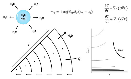
The study of respiratory droplets evaporation and formation of crystalline solid residues has become more and more important with the spread of respiratory diseases such as COVID-19. Evaporation time and droplet sizes greatly influence the dispersion of respiratory aerosols and their subsequent airborne transmission to susceptible hosts. In this study, a saline droplet is used as a surrogate for a respiratory droplet and a mathematical model is developed for its evaporation. Predictions agree well with experimental data reported in the literature. The model includes partial differential equations (PDEs) for the diffusion of dissolved solute and heat conduction within a saline droplet and water evaporation from the droplet surface. The internal domain of the droplet is discretized in space using the finite volume method, transforming the (PDEs) into a set of ordinary differential equations in time, which are solved using the Rosenbrock method. The calculation terminates when the solute concentration at the droplet surface reaches a value corresponding to a critical supersaturation level for the on-set of crystallization. The radial concentration profiles at different time intervals highlight the solute concentration enrichment at the droplet surface as it dries, by which the rate of solvent evaporation is affected. The model is also applied to a free-falling saline droplet evaporating under room temperature and relative humidity. The outcome reveals a strong dependency of the initial solute concentration on the ratio of initial to final droplet size. Lastly, the capability of the model predictions is demonstrated at a high relative humidity, where condensation occurs, broadening the model’s applicability.

GRAPHICAL ABSTRACT

Editor:

• Cari Dutcher

1. Introduction

1.1. Background

The COVID-19 pandemic has sparked considerable interest in the understanding of the mechanisms for the transmission of the disease. Among the three primary routes, airborne transmission of exhaled droplets has emerged as the predominant mode for the spread of SARS-CoV-2 (Anderson et al. 2020; Asadi et al. 2020; Morawska and Cao 2020). The initial size of respiratory droplets is one of the determining factors affecting dispersion, deposition and survival of the virus within the droplets. Based on the Wells evaporation curve (Wells 1934), large droplets (>100 µm) rapidly settle onto surfaces, whilst smaller ones evaporate to leave a solid residue (droplet nucleus) which can remain in the air for long periods of time before finally impinging and settling onto surfaces.

Once exhaled into the atmosphere, respiratory droplets flow with the air circulation and undergo heat and mass transfer with the air, shrink to droplet nuclei containing viral clusters, and ultimately cause the airborne transmission. The evaporation of water from these droplets and the resulting formation of a solid residue play a significant role in the dispersion of aerosols and subsequent disease transmission. This evaporation is greatly affected by the presence of dissolved solids such as salts, proteins and pathogens within the droplet (Vejerano and Marr 2018).

The study of droplet evaporation/drying extends beyond the field of respiratory diseases, with applications in spray drying, for example, in the pharmaceutical, detergent and food industries and in spray combustion. A comprehensive understanding of the drying process of droplets is therefore essential for accurate modeling and prediction of aerosol dispersion for respiratory disease control strategies, but also for industrial applications.

1.2. Previous studies

Mathematical models of various complexities have been developed to study the evaporation of respiratory droplets with different compositions (see reviews by Mao et al. 2020; Pourfattah et al. 2021). Saline droplets have frequently been used as surrogate for a respiratory droplet in evaporation modeling (Xie et al. 2007; Hardy et al. 2023) extending on a model initially developed for atmospheric aerosols (Kukkonen, Vesala, and Kulmala 1989). More sophisticated models have included multiple dissolved solutes to take into account the complexity of respiratory droplets composition (Redrow et al. 2011; De Oliveira et al. 2021). Recently, Hardy et al. (2023) extensively validated predictions from their model for the evaporation of binary droplets against data obtained from accurate measurements on droplet drying using a comparative-kinetics electrodynamic balance (CK-EDB) and a falling droplet column. These included both levitating and free-falling droplets experiments, particularly focusing on aqueous solutions of sodium chloride. However, this model assumed uniform solute concentration and temperature distributions inside the droplet and neglected the potential surface enrichment of the solute due to the shrinking of the droplet size. Inclusion of such phenomena greatly increase the mathematical complexity of the modeling caused by a moving boundary. Consequently, these models cannot account for the onset of solid residue formation in a supersaturated solution with solute concentration greater than the saturation concentration in the proximity of the surface of the droplet.

To address non-uniform solute concentration distribution inside the droplet, previous studies have either used a multi-shell approach to account for internal heat and mass transfer (Parienta et al. 2011) or applied a finite difference scheme in conjunction with measured variation in droplet size as a function of time to solve the diffusion equation (Gregson et al. 2019) or used an analytical method stating that the change in droplet radius is slow enough to consider the solute concentration profile inside the droplet as the stationary solution of the solute diffusion equation (Rezaei and Netz 2021). Some limitations were identified in these studies, such as the numerical accuracy of the solutions due to the use of a small number of computational shells (typically 8), the assumption of constant thermo-physical properties of the solvent, solutes and air or that the necessary information on the diffusivity of the solute or the vapor pressure at the droplet surface was not provided. Additionally, solving the diffusion and heat conduction equations analytically means that coupling between the heat and mass transfer is not possible, because the solute diffusivity is dependent on the temperature according to the Stokes-Einstein equation. While Gregson et al. (2019) developed a correlation for the diffusion coefficient of salt as a function of its mass fraction using dynamic viscosity measurements, the change in temperature within the droplet due to evaporative cooling was neglected in the modeling while it had an effect on the diffusion coefficient of sodium chloride.

In the field of spray drying, more emphasis has been placed in the numerical modeling of solute concentration and temperature distributions in an evaporating droplet. The numerical solution of the diffusion equation in spherical coordinates has been facilitated by the transformation into a “solute fixed coordinate system” by van der Lijn (1976) and this approach has been implemented by others (Adhikari, Howes, and Bhandari 2007; Ali et al. 2017). However, this method does not account for the temperature variation inside the droplet and cannot be extended to multi-component droplets. Sadafi et al. (2014) solved the heat conduction equation inside an aqueous sodium chloride solution droplet as it evaporates, but did not consider the non-uniform solute concentration distribution. Moreover, the temperature profiles within the droplet were not shown in the results, despite being the main attribute of the modeling. In other studies, the partial differential equations (PDEs) for both concentration and temperature variations within the droplet have been transformed into ordinary differential equations (ODEs) and solved using existing codes from the NAG Numerical Library (Seydel, Blömer, and Bertling 2006; Handscomb, Kraft, and Bayly 2009). Similarly, studies have used a finite volume method to convert the PDEs into ODEs, but provided minimal details regarding the discretization technique, which limits their applicability (Abdullahi, Burcham, and Vetter 2020; Poozesh et al. 2022). These studies have employed an explicit fourth or fifth order Runge-Kutta solver, suggesting that the set of ODEs might have been non-stiff. ODE stiffness arises when standard numerical methods to solve the differential equations such as explicit solvers are numerically unstable, except by reducing the step size significantly.

1.3. Present contributions

In this study, a first principle based distributed parameter model, which accommodates the internal transport of heat and mass within the droplet, is proposed to simulate the solvent (water) evaporation from stationary and free-falling saline droplets, serving as a surrogate for a respiratory droplet. The transport equations are discretized using a finite volume method, with description of all the derived equations provided in the online Supplemental Information (Sections S.1 and S.2). The model is parametrized using accurate thermodynamic, physical and chemical property data from the literature, which are crucial for the validity of the model and are summarized in Table 1. Firstly, the model is benchmarked by predicting published experimental data (Gregson et al. 2019; Gregson 2020; Hardy et al. 2023) and then the influence of initial droplet conditions, such as the size and solute concentration, on the evaporation rate and final droplet size is investigated. The model is also tested at high ambient relative humidity (RH) (60% and 100%), where the droplet acquires water through the process of condensation. The purpose of this study is to provide a validated evaporation model accounting for the effect of surface enrichment of the solute due to the shrinking of the droplet, as well as the heat conduction, providing a modeling framework for respiratory droplets containing multiple components. All the mathematical tools, such as derivations and discretization of transport equations, numerical solution methods, formulae for the thermo-physical properties and the drying conditions are provided in detail, along with guidelines on how to adapt the model to relax certain assumptions (see Sections 2.1 and 3.7 and online Supplemental Information), for researchers in the field to reproduce this model and build upon it. To the best of our knowledge, no other studies reported models with such detailed information, while accounting for the solute diffusion and heat conduction.

Table 1. Formulae for properties used in the modeling.

Symbol	Description	Formula	Unit	References
${\mathrm{\lambda }}_g$	Thermal conductivity of air	$2.5\times {10}^{-2}$	$\mathrm{W}\mathrm{ }{\mathrm{m}}^{-1}\mathrm{ }{\mathrm{K}}^{-1}$	Parienta et al. (2011)
${\mathrm{\lambda }}_w$	Thermal conductivity of water	$-0.432\mathrm{ }+\mathrm{ }5.725\times {10}^{-3}\mathrm{ }T\mathrm{ }‐\mathrm{ }8.078\mathrm{ }\times {10}^{-6}\mathrm{ }{\mathrm{T}}^2+\mathrm{ }1.861\times {10}^{-9}\mathrm{ }{\mathrm{T}}^3$	$\mathrm{W}\mathrm{ }{\mathrm{m}}^{-1}\mathrm{ }{\mathrm{K}}^{-1}$	Perry and Green (1997)
${\mathrm{\Phi }}_s$	Osmotic coefficient	Semi-empirical parametrisation (see Supplemental Information Section S.3.1)	–	Pitzer (1973)
$\mathrm{\mu }$	Viscosity of water	$-1.748\times {10}^{-5}\left(T-273\right)+1.336\times {10}^{-3}$	$\text{Pa s}$	Perry and Green (1997)
${\mathrm{\rho }}_p$	Density of saline droplet	$-2060{\mathrm{\omega }}^4+2252{\mathrm{\omega }}^3-3741{\mathrm{\omega }}^2+7410\mathrm{\omega }+997.1$	$\mathrm{\text{kg}}\mathrm{ }{\mathrm{m}}^{-3}$	Tang (1996)
$a_w$	Water activity of a saline droplet	$a_w=\mathrm{\text{exp}}\hspace{0.17em}\left(-\frac{2\mathrm{\omega }}{1‐\mathrm{\omega }}{\mathrm{\Phi }}_s \frac{M_w}{M_s}\right)$	–	Robinson and Stokes (2012)
$c_p$	Specific heat capacity	$15340.87-116.018 T+0.451 T^2-7.8\times {10}^{-4} T^3+5.2\times {10}^{-7} T^4$	$\text{J k}{\mathrm{g}}^{-1}\mathrm{ }{\mathrm{K}}^{-1}$	Perry and Green (1997)
$D$	Diffusion coefficient of salt in water	$D_0\frac{T}{293}\frac{\mathrm{\mu }\left(293\mathrm{ }\mathrm{K}\right)}{\mathrm{\mu }\left(\mathrm{T}\right)}$	${\mathrm{m}}^2\mathrm{ }{\mathrm{s}}^{-1}$	$D_0$ fitted from Gregson et al. (2019) (see Supplementary material Section S.3.2)
$D_g$	Diffusivity of water vapor in air	$\frac{0.001858 {\mathrm{T}}^{3/2}{\left({\mathrm{M}}_{\mathrm{w}}^{-1}+ {\mathrm{M}}_{\mathrm{\text{air}}}^{-1}\right)}^{0.5}}{\mathrm{p}{\mathrm{\sigma }}_{\mathit{\text{AB}}}^2{\mathrm{\Omega }}_D}$	${\mathrm{m}}^2\mathrm{ }{\mathrm{s}}^{-1}$	Brokaw (2002)
$h_{\mathit{\text{lg}}}$	Latent heat of vaporization of water	$2500.8-2.36\mathrm{T}+0.0016T^2-0.00006T^3$	$\text{J k}{\mathrm{g}}^{-1}$	Rogers and Yau (1989)
$\mathrm{\text{Nu}}$	Nusselt number	$2+{0.6\text{Re}}_{\mathrm{p}}^{1/2}{\text{Pr}}^{1/3}$	–	Ranz and Marshall (1952a)
$p_{\mathit{\text{sat}},T}$	Saturation vapor pressure of water	$610.8\mathrm{\text{exp}}\hspace{0.17em}\left(\frac{17.27\left(T-273.16\right)}{T-35.86}\right)$	$\mathrm{\text{Pa}}$	Bridgeman and Aldrich (1964)
$\mathrm{\text{Sh}}$	Sherwood number	$2+0.6\mathrm{R}{\mathrm{e}}_{\mathrm{p}}^{1\text{/}2}\mathrm{S}{\mathrm{c}}^{1\text{/}3}$	–	Ranz and Marshall (1952a)

2. Model formulation

2.1. Evaporation model

The first evaporation model for water droplets was developed by Maxwell in 1877 (Fuchs 1959) which serves as a basis for the development of the present model, with modifications to account for the presence of a solute. The following modeling assumptions are made:

• The droplet is considered spherical throughout the evaporation process,

• The evaporation of solvent (water) only causes diffusive motion of water vapor at the surface of the droplet, but no convective motion of water vapor in the air surrounding the droplet (Stefan flow),

• Circulation of solution within the droplet is neglected,

• The Kelvin effect due to the curvature of the droplet is neglected,

• The water vapor behaves as an ideal gas,

• The mass of solute remains constant during the evaporation.

In this case, the evaporation is governed by the water vapor concentration gradient between the surface of the droplet and far from the droplet. However, due to the presence of solutes, the water vapor pressure at the droplet surface will be lower than that of a pure water droplet, which is described by the water activity. Using a slightly modified version of the Maxwell model, taking account of the water activity of the droplet which depends on the concentration of solute at the surface, the change in droplet radius as a function of time can be written as: (1) $$\frac{\mathrm{d}{r}_p}{\mathrm{d}t}=\frac{M_w{D}_g\mathrm{ }\text{Sh}}{2r_p{\rho }_p}\left(\frac{\text{RH}{p}_{\mathit{\text{sat}},T_{\mathrm{\infty }}}}{R\mathrm{ }{T}_{\mathrm{\infty }}}-\frac{a_w{p}_{\mathit{\text{sat}},T_{\text{surf}}}}{R\mathrm{ }{T}_{\text{surf}}}\right)$$(1)

In Equation (1)(1) $$\frac{\mathrm{d}{r}_p}{\mathrm{d}t}=\frac{M_w{D}_g\mathrm{ }\text{Sh}}{2r_p{\rho }_p}\left(\frac{\text{RH}{p}_{\mathit{\text{sat}},T_{\mathrm{\infty }}}}{R\mathrm{ }{T}_{\mathrm{\infty }}}-\frac{a_w{p}_{\mathit{\text{sat}},T_{\text{surf}}}}{R\mathrm{ }{T}_{\text{surf}}}\right)$$(1) , $r_p$ is the droplet radius, ${\rho }_p$ its density, $D_g$ is the diffusivity of water vapor in air, $M_w$ is the molar weight of water, $\text{Sh}$ is the Sherwood number, $\text{RH}$ is the relative humidity, $T_{\mathrm{\infty }}$ is the temperature of the air, $T_{\mathit{\text{surf}}}$ is the temperature at the droplet surface and $a_w$ is the water activity.

2.2. Heat and mass transfer distributed parameter model

The solute diffusion and temperature distribution within the droplet are described by Fick’s second law (Equation (2)(2) $$\frac{\partial C}{\partial t}=\overrightarrow{\nabla }\cdot \left(D\overrightarrow{\nabla }C\right)$$(2) ) and the Fourier equation (Equation (3)(3) $$\frac{\partial T}{\partial t}=\overrightarrow{\nabla }\cdot \left(\mathrm{\kappa }\overrightarrow{\nabla }T\right)$$(3) ), respectively. In spherical coordinates, the solute concentration, $C,$ and solution temperature, $T,$ profiles are assumed to depend only on the radial position and not on the polar or azimuthal angles. At $t=0,$ both profiles are considered to be uniform (Equations (4)(4) $$C\left(r,t=0\right)=C_0$$(4) and (5)(5) $$T\left(r,t=0\right)=T_0$$(5) ). The boundary conditions at the droplet center are determined by the symmetry of the domain (Equations (6)(6) $${\left.\frac{\partial C}{\partial r}\right|}_{r=0}=0$$(6) and (7)(7) $${\left.\frac{\partial T}{\partial r}\right|}_{r=0}=0$$(7) ) and the boundary conditions at the droplet surface are given by Equations (8)(8) $${\left.\frac{\partial C}{\partial r}\right|}_{r=r_p}=\frac{-C\left(r_p\right)}{D}\frac{d r_p}{\mathit{\text{dt}}}$$(8) and (9)(9) $${\left.\frac{\partial T}{\partial r}\right|}_{r=r_p}=\frac{1}{2{\lambda }_w{r}_p}\left[\text{Nu}{\lambda }_g\left(T_{\mathrm{\infty }}-T_{\text{surf}}\right)+h_{\mathit{\text{lg}}}\frac{\dot{m_p}}{2\mathrm{\pi }{r}_p}\right]$$(9) , which are derived in the online Supplemental Information (Sections S.1.2 and S.2.2). (2) $$\frac{\partial C}{\partial t}=\overrightarrow{\nabla }\cdot \left(D\overrightarrow{\nabla }C\right)$$(2) (3) $$\frac{\partial T}{\partial t}=\overrightarrow{\nabla }\cdot \left(\mathrm{\kappa }\overrightarrow{\nabla }T\right)$$(3) (4) $$C\left(r,t=0\right)=C_0$$(4) (5) $$T\left(r,t=0\right)=T_0$$(5) (6) $${\left.\frac{\partial C}{\partial r}\right|}_{r=0}=0$$(6) (7) $${\left.\frac{\partial T}{\partial r}\right|}_{r=0}=0$$(7) (8) $${\left.\frac{\partial C}{\partial r}\right|}_{r=r_p}=\frac{-C\left(r_p\right)}{D}\frac{d r_p}{\mathit{\text{dt}}}$$(8) (9) $${\left.\frac{\partial T}{\partial r}\right|}_{r=r_p}=\frac{1}{2{\lambda }_w{r}_p}\left[\text{Nu}{\lambda }_g\left(T_{\mathrm{\infty }}-T_{\text{surf}}\right)+h_{\mathit{\text{lg}}}\frac{\dot{m_p}}{2\mathrm{\pi }{r}_p}\right]$$(9)

In Equations (2–9), $C$ is the concentration of solute, $T$ is the temperature inside the droplet, $D$ is the diffusivity of solute in water and $\kappa$ is the thermal diffusivity, ${\lambda }_w$ and ${\lambda }_g$ are the thermal conductivities of water and air, respectively, $h_{\mathit{\text{lg}}}$ is the latent heat of vaporization of water, and $\dot{m_p}$ is the change in droplet mass as a function of time that can be calculated using Equation (1)(1) $$\frac{\mathrm{d}{r}_p}{\mathrm{d}t}=\frac{M_w{D}_g\mathrm{ }\text{Sh}}{2r_p{\rho }_p}\left(\frac{\text{RH}{p}_{\mathit{\text{sat}},T_{\mathrm{\infty }}}}{R\mathrm{ }{T}_{\mathrm{\infty }}}-\frac{a_w{p}_{\mathit{\text{sat}},T_{\text{surf}}}}{R\mathrm{ }{T}_{\text{surf}}}\right)$$(1) , assuming that the change in droplet mass is only affected by the change in droplet radius and not by the change in droplet density: (10) $${\mathrm{ }\dot{m}}_p=\frac{\mathrm{d}{m}_p}{\mathrm{d}t}=4\mathrm{\pi }{\mathrm{\rho }}_p{r}_p^2\frac{\mathrm{d}{r}_p}{\mathrm{d}t}$$(10)

Equations (2)(2) $$\frac{\partial C}{\partial t}=\overrightarrow{\nabla }\cdot \left(D\overrightarrow{\nabla }C\right)$$(2) and (3)(3) $$\frac{\partial T}{\partial t}=\overrightarrow{\nabla }\cdot \left(\mathrm{\kappa }\overrightarrow{\nabla }T\right)$$(3) are discretized in space using the finite volume method in spherical coordinates. Following the mass and energy conservation on the control volume (also referred to as a cell), a normalization of the radial position is performed in order to obtain control volumes in the new system of coordinates that are fixed in space (see online Supplemental Information Section S.1.4). This allows the transformation of the PDEs (Equations (2)(2) $$\frac{\partial C}{\partial t}=\overrightarrow{\nabla }\cdot \left(D\overrightarrow{\nabla }C\right)$$(2) and (3)(3) $$\frac{\partial T}{\partial t}=\overrightarrow{\nabla }\cdot \left(\mathrm{\kappa }\overrightarrow{\nabla }T\right)$$(3) ) into ODEs in time given by Equations (11)(11) $$\frac{\mathrm{d}{C}_i}{\text{dt}}=3\frac{D_{i,e}\left(C_{i+1}-C_i\right)r_{i+1/2}^2-D_{i,w}\left(C_i-C_{i-1}\right)r_{i-1/2}^2}{r_p^2\left(r_{i+1/2}^3-r_{i-1/2}^3\right)\mathrm{\Delta }r}+\frac{r_i}{r_p}\frac{\mathrm{d}{r}_p}{\mathrm{d}t}\frac{C_{i+1}-C_{i-1}}{2\mathrm{\Delta }r}$$(11) and (12)(12) $$\frac{\mathrm{d}{T}_i}{\text{dt}}=3\frac{{\mathrm{\kappa }}_{i,e}\left(T_{i+1}-T_i\right)r_{i+1/2}^2-{\mathrm{\kappa }}_{i,w}\left(T_i-T_{i-1}\right)r_{i-1/2}^2}{r_p^2\left(r_{i+1/2}^3-r_{i-1/2}^3\right)\mathrm{\Delta }r}+\frac{r_i}{r_p}\frac{\mathrm{d}{r}_p}{\mathrm{d}t}\frac{T_{i+1}-T_{i-1}}{2\mathrm{\Delta }r}$$(12) . The boundary conditions are used to define fictitious points to extend the applicability of these equations for the cells closest to the droplet center and the droplet surface (Equations (13)(13) $${{\mathit{C}}_0={\mathit{C}}_1\mathit{\text{ and C}}}_{\mathit{M}+1}={\mathit{C}}_{\mathit{M}}‐r_p\mathit{\Delta }\mathit{r}\frac{{\mathit{C}}_{\mathit{M},\mathit{e}}}{\mathit{D}}\frac{\mathit{d}{\mathit{r}}_{\mathit{p}}}{\mathit{\text{dt}}}$$(13) and (14)(14) $${\mathit{T}}_0={\mathit{T}}_1 \mathit{\text{and}} {\mathit{T}}_{\mathit{M}+1}={\mathit{T}}_{\mathit{M}}+\frac{\text{Δr}}{2{\mathit{\lambda }}_{\mathit{w}}{\mathit{r}}_{\mathit{p}}}\left[\mathit{\text{Nu}}{\mathit{\lambda }}_{\mathit{g}}\left({\mathit{T}}_{\mathit{\infty }}-{\mathit{T}}_{\mathit{M},\mathit{e}}\right)+{\mathit{h}}_{\mathit{\text{lg}}}\frac{\dot{m_p}}{2\mathit{\pi }{r}_p}\right]$$(14) ). Central differences are used for the approximation of all derivatives. Diffusivities at the cell boundaries are calculated by taking the average of the values of diffusivity at the nodal points in two adjacent cells and the values of diffusivity, concentration or temperature at the droplet surface are computed using a first order extrapolation (see online Supplemental Information Section S.1.5). All the details of the derivations of Equations (11–14) are given in the online Supplemental Information (Sections S.1 and S.2). (11) $$\frac{\mathrm{d}{C}_i}{\text{dt}}=3\frac{D_{i,e}\left(C_{i+1}-C_i\right)r_{i+1/2}^2-D_{i,w}\left(C_i-C_{i-1}\right)r_{i-1/2}^2}{r_p^2\left(r_{i+1/2}^3-r_{i-1/2}^3\right)\mathrm{\Delta }r}+\frac{r_i}{r_p}\frac{\mathrm{d}{r}_p}{\mathrm{d}t}\frac{C_{i+1}-C_{i-1}}{2\mathrm{\Delta }r}$$(11) (12) $$\frac{\mathrm{d}{T}_i}{\text{dt}}=3\frac{{\mathrm{\kappa }}_{i,e}\left(T_{i+1}-T_i\right)r_{i+1/2}^2-{\mathrm{\kappa }}_{i,w}\left(T_i-T_{i-1}\right)r_{i-1/2}^2}{r_p^2\left(r_{i+1/2}^3-r_{i-1/2}^3\right)\mathrm{\Delta }r}+\frac{r_i}{r_p}\frac{\mathrm{d}{r}_p}{\mathrm{d}t}\frac{T_{i+1}-T_{i-1}}{2\mathrm{\Delta }r}$$(12) (13) $${{\mathit{C}}_0={\mathit{C}}_1\mathit{\text{ and C}}}_{\mathit{M}+1}={\mathit{C}}_{\mathit{M}}‐r_p\mathit{\Delta }\mathit{r}\frac{{\mathit{C}}_{\mathit{M},\mathit{e}}}{\mathit{D}}\frac{\mathit{d}{\mathit{r}}_{\mathit{p}}}{\mathit{\text{dt}}}$$(13) (14) $${\mathit{T}}_0={\mathit{T}}_1 \mathit{\text{and}} {\mathit{T}}_{\mathit{M}+1}={\mathit{T}}_{\mathit{M}}+\frac{\text{Δr}}{2{\mathit{\lambda }}_{\mathit{w}}{\mathit{r}}_{\mathit{p}}}\left[\mathit{\text{Nu}}{\mathit{\lambda }}_{\mathit{g}}\left({\mathit{T}}_{\mathit{\infty }}-{\mathit{T}}_{\mathit{M},\mathit{e}}\right)+{\mathit{h}}_{\mathit{\text{lg}}}\frac{\dot{m_p}}{2\mathit{\pi }{r}_p}\right]$$(14)

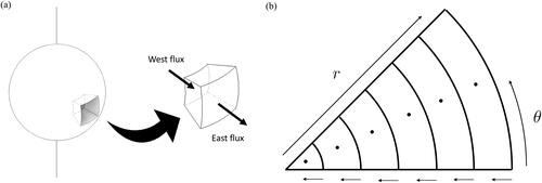
In Equations (11–14), $r$ is the normalized radial position. The droplet is divided into $M$ control volumes with central nodal points represented by the index $i$ ranging from $1$ to $M,$ as illustrated in Figure 1. The subscripts $e$ and $w$ correspond to the east and west boundary of each control volume, respectively. The convention adopted in this study is that the cell closest to the droplet center corresponds to the most western cell and the cell closest to the droplet surface is the most eastern cell. The indices $i=0$ and $i=M+1$ refer to fictitious points which are outside the domain and are only used for the purpose of extending Equations (11)(11) $$\frac{\mathrm{d}{C}_i}{\text{dt}}=3\frac{D_{i,e}\left(C_{i+1}-C_i\right)r_{i+1/2}^2-D_{i,w}\left(C_i-C_{i-1}\right)r_{i-1/2}^2}{r_p^2\left(r_{i+1/2}^3-r_{i-1/2}^3\right)\mathrm{\Delta }r}+\frac{r_i}{r_p}\frac{\mathrm{d}{r}_p}{\mathrm{d}t}\frac{C_{i+1}-C_{i-1}}{2\mathrm{\Delta }r}$$(11) and (12)(12) $$\frac{\mathrm{d}{T}_i}{\text{dt}}=3\frac{{\mathrm{\kappa }}_{i,e}\left(T_{i+1}-T_i\right)r_{i+1/2}^2-{\mathrm{\kappa }}_{i,w}\left(T_i-T_{i-1}\right)r_{i-1/2}^2}{r_p^2\left(r_{i+1/2}^3-r_{i-1/2}^3\right)\mathrm{\Delta }r}+\frac{r_i}{r_p}\frac{\mathrm{d}{r}_p}{\mathrm{d}t}\frac{T_{i+1}-T_{i-1}}{2\mathrm{\Delta }r}$$(12) to $i=1$ and $i=\mathrm{M}.$ The indices $i+1/2$ and $i-1/2$ correspond to the cell boundaries. Details on the use of fictitious points are given in the online Supplemental Information (Sections S.1.5 and S.2.3).

Figure 1. Representation of the control volume in spherical coordinates in (a) 3D and (b) 2D when M = 6.

2.3. Equations of droplet motion

The equations for the droplet motion are governed by Newton’s second law of motion. The forces acting on the droplet are due to drag, buoyancy and gravity. The droplet is considered to be moving in a 2D plane with one vertical and one horizontal coordinate, so four ODEs are needed to model the motion of a droplet, two for the droplet velocity (Equation (15)(15) $$\frac{\mathrm{d}\overrightarrow{{\mathit{u}}_{\mathit{p}}}}{\mathrm{d}t}=\frac{\overrightarrow{{\mathbf{u}}_{\mathbf{g}}}-\overrightarrow{{\mathit{u}}_{\mathit{p}}}}{{\tau }_p}+\left(1-\frac{{\rho }_g}{{\rho }_p}\right)\overrightarrow{g}$$(15) ) and two for the droplet position (Equation (16)(16) $$\frac{\mathrm{d}\overrightarrow{{\mathit{x}}_{\mathit{p}}}}{\mathrm{d}t}=\overrightarrow{{\mathit{u}}_{\mathit{p}}}$$(16) ). (15) $$\frac{\mathrm{d}\overrightarrow{{\mathit{u}}_{\mathit{p}}}}{\mathrm{d}t}=\frac{\overrightarrow{{\mathbf{u}}_{\mathbf{g}}}-\overrightarrow{{\mathit{u}}_{\mathit{p}}}}{{\tau }_p}+\left(1-\frac{{\rho }_g}{{\rho }_p}\right)\overrightarrow{g}$$(15) (16) $$\frac{\mathrm{d}\overrightarrow{{\mathit{x}}_{\mathit{p}}}}{\mathrm{d}t}=\overrightarrow{{\mathit{u}}_{\mathit{p}}}$$(16)

In Equations (15)(15) $$\frac{\mathrm{d}\overrightarrow{{\mathit{u}}_{\mathit{p}}}}{\mathrm{d}t}=\frac{\overrightarrow{{\mathbf{u}}_{\mathbf{g}}}-\overrightarrow{{\mathit{u}}_{\mathit{p}}}}{{\tau }_p}+\left(1-\frac{{\rho }_g}{{\rho }_p}\right)\overrightarrow{g}$$(15) and (16)(16) $$\frac{\mathrm{d}\overrightarrow{{\mathit{x}}_{\mathit{p}}}}{\mathrm{d}t}=\overrightarrow{{\mathit{u}}_{\mathit{p}}}$$(16) , ${\tau }_p$ is the droplet relaxation time which depends on the droplet Reynolds number $\mathrm{R}{\mathrm{e}}_{\mathrm{p}},$ the Cunningham slip correction factor $C_c$ and the drag coefficient $C_d,$ which is based on an empirical correlation (Schiller and Naumann 1935), and given by: $${{\tau }_p\mathrm{ }=\mathrm{ }\frac{C_c\mathrm{ }{\rho }_p\mathrm{ }{d}_p^2}{18\mathrm{ }{\mu }_g}\mathrm{ }\frac{24}{C_d\mathrm{ }{\text{Re}}_p}\text{Re}}_p=\frac{{\mathrm{\rho }}_g{d}_p\left|\overrightarrow{u_g}-\overrightarrow{u_p}\right|}{{\mathrm{\mu }}_g} C_c=1+K_n\left(1.257+0.4\mathrm{\text{exp}}\hspace{0.17em}\left(\frac{-1.1}{K_n}\right)\right)$$ $${C_d=\frac{24}{{\text{Re}}_p}\text{for Re}\mathrm{<}\text{1}C}_d=\frac{24}{{\text{Re}}_p}\left(1+0.15{\text{Re}}_p^{0.687}\right)$$

2.4. Numerical solution method

The equation for the change in droplet radius (Equation (1)(1) $$\frac{\mathrm{d}{r}_p}{\mathrm{d}t}=\frac{M_w{D}_g\mathrm{ }\text{Sh}}{2r_p{\rho }_p}\left(\frac{\text{RH}{p}_{\mathit{\text{sat}},T_{\mathrm{\infty }}}}{R\mathrm{ }{T}_{\mathrm{\infty }}}-\frac{a_w{p}_{\mathit{\text{sat}},T_{\text{surf}}}}{R\mathrm{ }{T}_{\text{surf}}}\right)$$(1) ), the $M$ equations for both the solute concentration (Equation (11)(11) $$\frac{\mathrm{d}{C}_i}{\text{dt}}=3\frac{D_{i,e}\left(C_{i+1}-C_i\right)r_{i+1/2}^2-D_{i,w}\left(C_i-C_{i-1}\right)r_{i-1/2}^2}{r_p^2\left(r_{i+1/2}^3-r_{i-1/2}^3\right)\mathrm{\Delta }r}+\frac{r_i}{r_p}\frac{\mathrm{d}{r}_p}{\mathrm{d}t}\frac{C_{i+1}-C_{i-1}}{2\mathrm{\Delta }r}$$(11) ) and the solution temperature (Equation (12)(12) $$\frac{\mathrm{d}{T}_i}{\text{dt}}=3\frac{{\mathrm{\kappa }}_{i,e}\left(T_{i+1}-T_i\right)r_{i+1/2}^2-{\mathrm{\kappa }}_{i,w}\left(T_i-T_{i-1}\right)r_{i-1/2}^2}{r_p^2\left(r_{i+1/2}^3-r_{i-1/2}^3\right)\mathrm{\Delta }r}+\frac{r_i}{r_p}\frac{\mathrm{d}{r}_p}{\mathrm{d}t}\frac{T_{i+1}-T_{i-1}}{2\mathrm{\Delta }r}$$(12) ) distributions and the four equations for the droplet motion (Equations (15)(15) $$\frac{\mathrm{d}\overrightarrow{{\mathit{u}}_{\mathit{p}}}}{\mathrm{d}t}=\frac{\overrightarrow{{\mathbf{u}}_{\mathbf{g}}}-\overrightarrow{{\mathit{u}}_{\mathit{p}}}}{{\tau }_p}+\left(1-\frac{{\rho }_g}{{\rho }_p}\right)\overrightarrow{g}$$(15) and (16)(16) $$\frac{\mathrm{d}\overrightarrow{{\mathit{x}}_{\mathit{p}}}}{\mathrm{d}t}=\overrightarrow{{\mathit{u}}_{\mathit{p}}}$$(16) ) form a system of $2M+5$ ODEs. Due to the difference in timescales of the processes involved (evaporation, solute diffusion, heat conduction and droplet motion), these ODEs behave at significantly different rates and the system therefore is stiff. In general, ODE stiffness increases with the number of nodal points (Schiesser and Griffiths 2009), meaning that an optimal number is crucial. Moreover, when dealing with stiffness, a careful choice of the time step size (Δt) is essential for achieving stability (Lindfield and Penny 2018).

Because of the degree of instability caused by the stiffness of the ODEs, an implicit method is needed to solve these equations (Hairer and Wanner 1991). In this study, a four-stage Rosenbrock method is used with an automatic time step adjustment algorithm (Rosenbrock 1963; Press et al. 1992). It involves solving multiple linear equations at each time step in order to approximate the solution of the non-linear equations needed for the implicit method.

The numerical integration is terminated when the solute (sodium chloride) concentration at the surface of the droplet reaches a supersaturation (S) level (defined as the ratio of the concentration of sodium chloride to the equilibrium solubility) above $2.04.$ This has been shown to be the point for the on-set of crystallization in a saline droplet based on the experimental data combined with numerical modeling of Gregson et al. (2019). Furthermore, the calculations are also terminated when the droplet radius falls to 0.5 µm even if the specified supersaturation level has not been reached. This way, the Knudsen number (Kn), defined as the ratio of the molecular mean free path length to the droplet radius, always remains above the transitional value of $0.1,$ so the droplet can be considered to be in the continuum regime.

2.5. Properties of the solute, solvent and air

The formulae for the thermodynamic, physical and chemical properties as a function of temperature or solute concentration employed in the model are given in Table 1, along with references. Therein, the temperature $T$ is given in K, $\omega$ is the mass fraction of solute, $p$ the total pressure in atm, ${\mathrm{\sigma }}_{\mathit{\text{AB}}}$ and ${\Omega }_D$ are the collision diameter in angstrom and collision integral in the Chapman–Enskog theory, respectively.

In this study, the simplifying assumption of volume additivity for an aqueous solution of water and NaCl is relaxed. Instead, the density of the droplet as a function of the mass fraction of solute is based on empirical parametrisations to provide more accurate results (Tang 1996). Similarly, the osmotic coefficient uses a semi-empirical parametrisation as a function of the mass fraction of solute (Pitzer 1973) to calculate the water activity of the droplet as described in the online Supplemental Information (Section S.3.1). The diffusion coefficient of NaCl in water is fitted based on the data from Gregson et al. (2019) (online Supplemental Information, Section S.3.2), which has been calibrated from dynamic viscosity measurements. The Stokes-Einstein equation can also be used to calculate the diffusion coefficient, however at high concentrations the values may be orders of magnitude off from the actual value (de Souza Lima, Ré, and Arlabosse 2020). Therefore, the empirical fit to the data of Gregson et al. (Gregson et al. 2019) is used in combination with the Stokes-Einstein equation to calculate the diffusion coefficient at different temperatures.

3. Results and discussion

3.1. Validation of pure water droplet evaporation model

As a first step, the evaporation model is validated for a stationary pure water droplet, therefore removing the need to solve all the differential equations for the solute diffusion. Additionally, the temperature is considered as uniform inside the droplet in this model to simplify the problem. Under this condition, only two ODEs need to be solved, as the droplet is stationary: one for the evaporation from the droplet and the resulting change in the radius as described in Equation (1)(1) $$\frac{\mathrm{d}{r}_p}{\mathrm{d}t}=\frac{M_w{D}_g\mathrm{ }\text{Sh}}{2r_p{\rho }_p}\left(\frac{\text{RH}{p}_{\mathit{\text{sat}},T_{\mathrm{\infty }}}}{R\mathrm{ }{T}_{\mathrm{\infty }}}-\frac{a_w{p}_{\mathit{\text{sat}},T_{\text{surf}}}}{R\mathrm{ }{T}_{\text{surf}}}\right)$$(1) and the other for the heat transfer that results from an energy balance on the droplet as it evaporates (Crowe et al. 2011): (17) $$\frac{\mathrm{d}{T}_p}{\mathrm{d}t}=\frac{3}{2r_p^2{\mathrm{\rho }}_p{c}_p}\left[{\lambda }_g\mathrm{ }\text{Nu}\left(T_{\mathrm{\infty }}-T_p\right)+h_{\mathit{\text{lg}}}\frac{\dot{m_p}}{2\mathit{\pi }{r}_p}\right]$$(17)

This system of two coupled non-linear ODEs is solved using a numerical adaptive time-step explicit Runge-Kutta (RK) method (Dormand and Prince 1980), which evaluates the solution using both a four-stage and five-stage RK algorithm and considers the local truncation error to be the difference between the solutions from these evaluations. This estimation of the error is then compared to a pre-defined tolerance threshold, and determines whether the time step is valid or requires reevaluation of the numerical solution, depending on the error being below or above the threshold. The time step size is then reduced or increased in order to improve accuracy and/or save on computational time.

The predictions from the model are presented in Figure 2 along with the experimental data from the literature using the same initial and ambient air conditions (Ranz and Marshall 1952b; Hardy et al. 2023). The square of the normalized droplet diameter follows a straight line when plotted against time, in accordance with the $d^2$-law (Langmuir 1918). The time is made dimensionless by dividing it by an evaporation timescale ${\tau }_{\mathit{\text{evap}}}$ defined by Equation (18)(18) $${\mathrm{\tau }}_{\mathit{\text{evap}}}=\frac{r_{p0}^2{\mathrm{\rho }}_{p}R}{\text{Sh}{D}_g{M}_w}{\left(\frac{p_{\mathit{\text{sat}},T_0}}{T_0}-\frac{\text{RH}{p}_{\mathit{\text{sat}},T_{\mathrm{\infty }}}}{T_{\mathrm{\infty }}}\right)}^{-1}$$(18) , which represents an estimate of the time for a pure water droplet to fully evaporate should its properties (temperature, velocity) remain unchanged during the evaporation, and is therefore based on the ambient and initial conditions only. The derivation of ${\tau }_{\mathit{\text{evap}}}$ is given in the online Supplemental Information (Section S.3.4). (18) $${\mathrm{\tau }}_{\mathit{\text{evap}}}=\frac{r_{p0}^2{\mathrm{\rho }}_{p}R}{\text{Sh}{D}_g{M}_w}{\left(\frac{p_{\mathit{\text{sat}},T_0}}{T_0}-\frac{\text{RH}{p}_{\mathit{\text{sat}},T_{\mathrm{\infty }}}}{T_{\mathrm{\infty }}}\right)}^{-1}$$(18)

Figure 2. Change in droplet size with time for a pure water droplet under different conditions compared with experimental data from the literature.

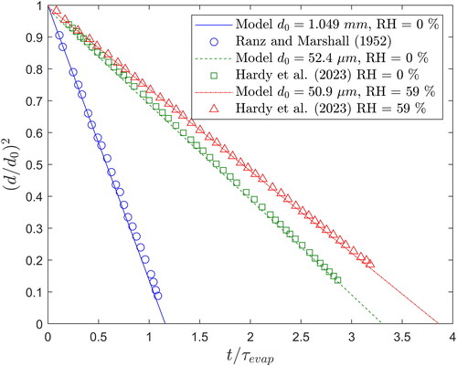
For the comparison with the Ranz and Marshall (1952b) experiments, $d_0=1.049$ mm $T_0=282\hspace{0.17em}\mathrm{K}\mathrm{ }(9°C),$ $T_{\mathrm{\infty }}=298\hspace{0.17em}\mathrm{K} (25°C)$ and RH = 0% (dry air), the total evaporation time is very close to the evaporation timescale ${\tau }_{\mathit{\text{evap}}}$ (Equation (18)(18) $${\mathrm{\tau }}_{\mathit{\text{evap}}}=\frac{r_{p0}^2{\mathrm{\rho }}_{p}R}{\text{Sh}{D}_g{M}_w}{\left(\frac{p_{\mathit{\text{sat}},T_0}}{T_0}-\frac{\text{RH}{p}_{\mathit{\text{sat}},T_{\mathrm{\infty }}}}{T_{\mathrm{\infty }}}\right)}^{-1}$$(18) ). This is due to the fact that the initial droplet temperature ($9°C$) is very close to its wet-bulb temperature ($7°C$) under the experimental conditions, so there is little change in the droplet temperature and the evaporation can be well represented by the $d^2$-law using the initial droplet conditions only. In the cases where $d_0=52.4 \mathrm{\mu }\mathrm{m}$ or $50.9 \mathrm{\mu }\mathrm{m},$ the initial droplet temperature is the same as the ambient air temperature ($20°C$), so there is a large reduction in the droplet temperature during the initial stage of evaporation. From comparison with each experiment, the model demonstrates excellent agreement with the measured data, which validates the evaporation model for a pure water droplet.

3.2. Sensitivity analysis of the numerical solution of the distributed parameter model

Two parameters affect the accuracy of the numerical results: the number of spatial cells $M$ and the error threshold $\mathrm{ϵ}$ used in the solution of the system of coupled non-linear ODEs. Two outputs are monitored to assess the accuracy of the numerical solution: the time to reach the supersaturation level of 2.04 and the ratio of the final to initial mass of NaCl, which should be equal to 1, as NaCl does not evaporate. At any time during the evaporation, the mass of solute can be calculated by the numerical integration (using the trapezoidal rule) of radial concentration profile, given by Equation (19)(19) $$m_s=4\pi {\int }_0^{r_p}C\left(r,t\right)r^2\mathrm{ }\text{dr}$$(19) : (19) $$m_s=4\pi {\int }_0^{r_p}C\left(r,t\right)r^2\mathrm{ }\text{dr}$$(19)

The results of a sensitivity analysis are given in Table 2 based on a levitating saline droplet with an initial diameter $d_0=45.72 \mathrm{\mu }\mathrm{m},$ an initial NaCl concentration of 24 g/L, ambient conditions of temperature at 20 °C and a RH of 0%. Based on these results, the number of cells $M=100$ and the error threshold $\mathrm{ϵ}={10}^{-5}$ are chosen for the numerical investigations. The selection of these parameters gives a ratio of final to initial mass of solute of 0.9997 and a time to reach S = 2.04 within $0.001 \mathrm{s}$ of the results with a larger $\mathrm{M}\mathrm{ }(=1000)$ or smaller $\mathrm{ϵ}\mathrm{ }(={10}^{-7}),$ so they are deemed sufficiently accurate. In this case, the computational time was in the order of one minute on a workstation with an Intel® X® W-2245 CPU at 3.90 GHz and 64 GB of RAM. Using an explicit RK method with adaptative time step described in the previous section, it would take 7 to 8 h, as the stiffness of the system of ODEs requires a very small time step in order to remain stable throughout the entirety of the calculation.

Table 2. Sensitivity analysis on number of cells and error threshold (bold font indicate the selected number of cells and tolerance threshold in the study).

Number of cells	Error threshold	Computational time (hh:mm:ss)	Time to reach S = 2.04 (s)	Ratio of final to initial mass of solute
10	10^-3	00:00:00	1.6495	0.9931
10	10^-5	00:00:01	1.6444	0.9975
10	10^-7	00:00:10	1.6421	0.9978
100	10^-3	00:00:10	1.6535	0.9957
100	10^-5	00:01:04	1.6417	0.9997
100	10^-7	00:10:05	1.6417	0.9999
1000	10^-3	00:21:45	1.6553	0.9947
1000	10^-5	02:33:10	1.6424	0.9997
1000	10^-7	23:41:00	1.6416	0.9999

3.3. Validation of stationary saline droplet evaporation model

The second step of the model validation focuses on stationary saline droplets, where the model predictions are compared with published experimental data on single levitating saline droplets in Figure 3a (Gregson et al. 2019) and Figure 3b (Gregson 2020). These experiments were carried out using a CK-EDB, which uses an electromagnetic field to levitate single droplets and the droplet size is monitored with time by light-scattering method. This technique has a high fidelity for single droplet evaporation measurements in the micrometre range compared to an acoustic levitator which produces waves that may affect the evaporation rate for such small droplets (Yarin et al. 1999). The predictions of the model are closely aligned with the experiments for both the cases at a RH of 0% and 42%.

Figure 3. Predicted change in size with time for stationary saline droplets compared with experimental data at (a) RH = 0% and (b) RH = 42%.

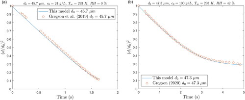
At the RH of 42%, the influence of the solute concentration on the evaporation is noticeable, as the drying curve (Figure 3b) deviates from a straight line in the later stage of evaporation. This is well represented in the model by the influence of the droplet water activity ${\mathrm{a}}_{\mathrm{w}}$ described in Section 2.5 and online Supplemental Information Section S.3.1. The effect is also observed at the RH of 0% (Figure 3a); however, due to the faster evaporation rate, it is less prominent.

In combination with their experimental measurements of droplet size, Gregson and coworkers used a finite difference discretization of an isothermal version of the solute diffusion equation (Equations (2–8)) to model the concentration distribution inside the droplet as it evaporates. Their model predictions along with those of this model are plotted in Figure 4, and correspond to the same conditions used to generate the predictions in Figure 3. The radial profiles of solute concentration for the conditions relating to Figure 3a are plotted against the changing radius during the time from the beginning of the evaporation until the moment when the surface concentration reaches the supersaturation level of 2.04 in Figure 4a. Notably, the plot reveals non-uniform concentration profiles, especially toward the end of the evaporation. The Peclet number (Pe), which compares the evaporation rate of the solvent to the diffusion rate of the solute, has often been used to describe whether the droplet remains homogenous or not during evaporation (Vehring 2008). A low Pe means that the solute diffuses faster than the droplet shrinks, and vice versa. However, a calculation of Pe for the situation presented in Figure 5a and Figure 6a (RH = 0%) reveals that it remains below 0.5 throughout the evaporation, indicating that despite a low Pe, surface enrichment of the solute can still be observed.

Figure 4. (a) Predicted solute concentration profiles at different times within a stationary saline droplet for RH = 0% and (b) concentration of solute at the droplet surface for RH = 42%.

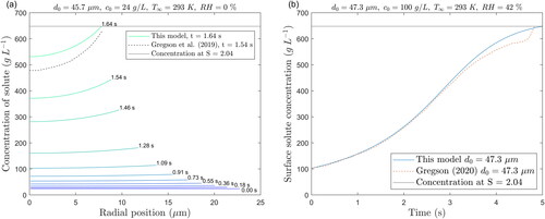
Figure 5. (a) Predicted and measured changes in size of falling saline droplets as a function of time at two RHs and (b) predicted change in temperature as a ′function of time at different radial positions for RH = 35%.

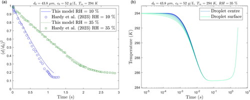
Figure 6. (a) Predicted change in droplet size at RH of 60% and 100% and (b) change in droplet surface temperature.

The present model predictions are relatively close to those obtained from the combined experimental and modeling approach of Gregson et al. (2019). The time to reach the critical supersaturation level S = 2.04 of the present model is within 6% to that of Gregson et al. (2019). However, the concentration profiles do differ at the time when the critical supersaturation is reached, but this may be due to the influence of the droplet temperature on the diffusion coefficient used in these models. In their model, Gregson et al. (2019) do not account for the temperature change as the droplet evaporates, which affects the diffusion coefficient following the Stokes-Einstein relation. Indeed, at 0% RH, the droplet temperature drops from 20 °C to 5 °C, which reduces the diffusivity of sodium chloride by 33%. Moreover, although quite close, the change in droplet size from the present model predictions does not match exactly the experimental values (see Figure 3a). This affects the rate at which the droplet surface shrinks and therefore the diffusion of solute. The surface concentration profiles shown in Figure 4b reveal that both predictions are very close until a certain point of time toward the end of the evaporation. This is already noticeable in the plot of droplet size as a function of time in Figure 3b. It is likely that the droplet is undergoing phase transformation, affecting the light scattering, or that the size of the droplet becomes too small to be accurately trapped by the electromagnetic field.

3.4. Evaporation of free-falling droplets

The final part of the model validation addresses the evaporation of free-falling droplets, where the equations of motion (Equations (15)(15) $$\frac{\mathrm{d}\overrightarrow{{\mathit{u}}_{\mathit{p}}}}{\mathrm{d}t}=\frac{\overrightarrow{{\mathbf{u}}_{\mathbf{g}}}-\overrightarrow{{\mathit{u}}_{\mathit{p}}}}{{\tau }_p}+\left(1-\frac{{\rho }_g}{{\rho }_p}\right)\overrightarrow{g}$$(15) and (16)(16) $$\frac{\mathrm{d}\overrightarrow{{\mathit{x}}_{\mathit{p}}}}{\mathrm{d}t}=\overrightarrow{{\mathit{u}}_{\mathit{p}}}$$(16) ) are involved and the Sherwood (Sh) and Nusselt (Nu) numbers (described in Table 1) are increased due to the droplet motion. The predictions are compared with the experimental data at two different RH in Figure 5a, sourced from a study utilizing a falling droplet column (Hardy et al. 2023). In their experimental setup, droplets were injected at regular intervals using a droplet dispenser. As the droplets fall through the column, a high-speed camera captures images at various vertical positions and records the trajectory and evaporation history of the droplets.

The predicted results at the RH of 35% indicate a better agreement with the experimental data than at RH = 10%. However, it is important to note that some measurement errors were reported in the original study. First, the apparent RH may only be accurate to ±5%, which has a great influence on the evaporation rate. Other measurement errors were associated with the droplet size ($\pm 0.4\text{ μm}$ at RH = 10% and $\pm 0.6\text{ μm}$ at RH = 35%), initial velocities ($\pm 0.2\text{ m }{\mathrm{s}}^{-1}$) and even ambient temperature ($\pm 1\mathrm{ }\mathrm{K}$). All combined, the differences between the actual and nominal values of the initial and ambient conditions may result in an over- or under-estimated evaporation rate.

For the case of 35% RH, the temperature variation with time at different locations along the droplet radius is presented in Figure 5b. The time is represented on a log-scale in order to show the comparison between the temperature profile at the droplet center and the droplet surface at the first moments of the evaporation. In less than $0.1 \mathrm{s},$ the temperature becomes uniform along the droplet radius. Two dimensionless numbers are generally used to ascertain the uniformity temperature profile inside a body. First the Biot number (Bi), representing the ratio of the internal conduction to the external convection resistances, and the Fourier number (Fo), which is the ratio of the time $t$ to a characteristic timescale for heat diffusion. In the case presented in Figure 6b, Bi is in the order of 0.1 for the entirety of the evaporation and Fo becomes larger than 10 within $0.1 \mathrm{s},$ confirming the rapid evolution of the temperature distribution to a uniform profile.

3.5. Influence of initial droplet size and concentration

The model is used to assess the effect of initial droplet size (1 to 100 µm) and solute concentration (1 to 200 g/L) on the time to reach S = 2.04 and the ratio of final to initial diameter. Table 3 lists the predictions for initial and ambient temperature corresponding to respiratory droplets in a typical indoor environment of $T_0=37°C,$ $T_{\mathrm{\infty }}=20°C$ and $\text{RH}=35\%.$

Table 3. Evaporation time and ratio of final to initial droplet size with varying initial diameters and solute concentrations.

Initial diameter (µm)	Initial solute concentration (g/L)	Time to reach S = 2.04 (s)	Ratio of final to initial diameter
1	1	0.0013	0.1160
10	1	0.1336	0.1161
100	1	11.27	0.1161
1	10	0.0014	0.2498
10	10	0.1406	0.2502
100	10	11.85	0.2501
1	50	0.0015	0.4272
10	50	0.1523	0.4268
100	50	12.54	0.4281
1	100	0.0016	0.5386
10	100	0.1570	0.5377
100	100	12.64	0.5394
1	200	0.0015	0.6783
10	200	0.1547	0.6775
100	200	12.04	0.6800

The initial diameter greatly influences the total evaporation time, showing a proportional relationship with the square of the initial diameter. Interestingly, the ratio of the final to initial diameters does not depend on the initial droplet size. The initial solute concentration, on the other hand, shows the opposite trend. The evaporation time does not change much with the initial concentration, but the ratio of final to initial droplet sizes is greatly affected by the initial concentration. Both of these findings reveal how important the initial conditions are in determining the final droplet sizes and the evaporation times. These are in agreement with the modeling results by Liu et al. (2017).

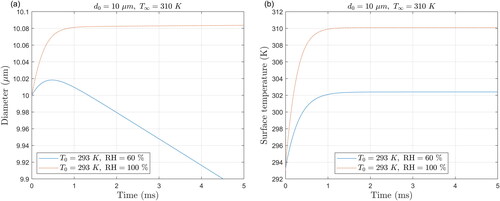
3.6. Application of the model to the evaporation droplets at high relative humidity

The model equations presented in Section 2.2 are also applicable if the droplet undergoes condensation due to hygroscopic growth instead of evaporation. This scenario could occur if a droplet enters a highly humid environment such as the mouth or the lungs. The changes in size of a stationary saline droplet with an initial diameter of $10 \mathrm{\mu }\mathrm{m}$ and an initial solute concentration of 10 g/L at relative humidities of 60% and 100% are depicted in Figure 6a, focusing on the first 5 ms. In these simulations, the initial droplet temperatures are set to 20 °C (room temperature), while the ambient temperature is set to 37 °C (typical body temperature). These two situations are similar to a previous study on the evaporation/condensation of pure water (Redrow et al. 2011).

In contrast to the results at lower RH values (Figure 5b), the temperature of the droplet at high RHs increases (Figure 6b) until reaching the wet-bulb temperature, which at a RH of 100% is the same as the ambient temperature. At 60% RH, the droplet first grows due to condensation and the rise in the droplet temperature increases the water vapor pressure at its surface, which eventually becomes higher than that of the ambient air. The droplet size then decreases at a steady rate when the variation of the droplet temperature becomes sufficiently small as it reaches the wet-bulb temperature.

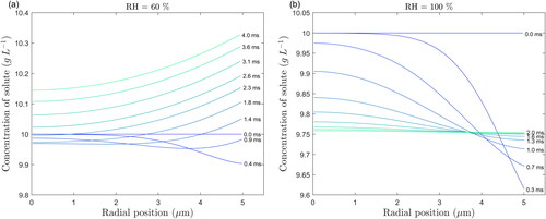
At the RH of 60%, the solute concentration at the droplet surface (Figure 7a) first decreases due to condensation and then increases due to evaporation, as expected following the trend of variation of droplet size with time (Figure 6a). However, because the diffusion of solute is not instantaneous, the concentration does not reach a uniform profile before the droplet size begins to decrease. This leads to the formation of a wave in the profile, particularly visible at 0.9 ms. At the RH of 100%, the solute concentration decreases and eventually reaches a uniform profile (Figure 7b) due to the droplet temperature and size becoming constant (Figure 6a,b). These cases demonstrate the capability of the model to handle both condensation and evaporation, even when both processes occur for the same droplet.

Figure 7. Predicted radial profiles of solute concentration at (a) RH = 60% and (b) RH = 100%.

3.7. The effects of model assumptions on the predictions

The models developed in this study are based on the assumptions outlined in Section 2.1, which are only applicable in specific circumstances. First, the Stefan flow, an outward flow of water vapor from the droplet surface during evaporation, is not accounted for. This means that the evaporation of the solvent at the surface of the droplet is governed by diffusion only, and not by convective motion of water vapor, which is valid for slowly evaporating droplets. The criterion to check whether this assumption is applicable or not is given by Seinfeld and Pandis (2016) as: (20) $$\frac{D_g}{{\mathrm{\kappa }}_{\mathit{\text{air}}}}\frac{M_w}{M_{\mathit{\text{air}}}}\mathrm{l}\mathrm{n}\left(\frac{1-x_{w,s}}{1-x_{w,\mathrm{\infty }}}\right)\ll 1,$$(20) where $x_{w,s}$ and $x_{w,\infty }$ are the mole fraction of water at the droplet surface and far from the droplet, respectively. In the experimental cases simulated in this study, the criterion is of the order of ${10}^{-4},$ which is far below 1 and therefore the Stefan flow can be neglected.

Another assumption made concerns the Kelvin effect, which has been neglected. The effect, whereby the vapor pressure over the curved surface of a droplet is greater than that over a flat plane, is negligible for droplets larger than $0.2 \mathrm{\mu }\mathrm{m}$ (Seinfeld and Pandis 2016). Similarly, the droplet size is much larger than the mean free path of the gas molecules. Therefore, the Knudsen number (Kn), defined as the ratio of the molecular mean free path length to the droplet radius, is below 0.1 throughout the evaporation in all cases investigated here, so the system under consideration (droplet and air) is in the continuum regime. For droplet sizes smaller than a few micrometers, the system becomes transitional and requires a correction factor for the evaporation model with the use of an accommodation coefficient (Seinfeld and Pandis 2016).

The circulation of liquid inside droplets is generally neglected, as it only occurs if the Bond (or Eötvös) number (Bo or Eo) is above 4, known as the Bond criterion (Clift, Grace, and Weber 1978). This dimensionless number compares the gravitational to the capillary forces, and for all droplets considered in this study, it is always below 0.2.

The droplet temperature distributions are obtained using the thermal properties, such as the heat capacity, thermal conductivity and latent heat, of pure water and do not account for the influence of a dissolved solute. Based on the results of temperature variation with time (Figure 5b), this would have little impact, because the temperature profile becomes uniform within a very short time. Furthermore, the heat transfer due to radiation at the droplet surface is neglected in the boundary conditions and is considered to make minimal contribution to the change in droplet temperature (Sazhin 2006).

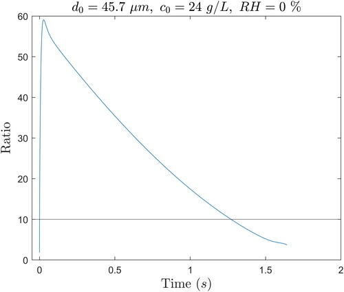
In order not to further complicate an already complex mathematical problem, the term containing the derivative of the density was not accounted for in the calculation of the derivative of the droplet mass shown in Equation (10)(10) $${\mathrm{ }\dot{m}}_p=\frac{\mathrm{d}{m}_p}{\mathrm{d}t}=4\mathrm{\pi }{\mathrm{\rho }}_p{r}_p^2\frac{\mathrm{d}{r}_p}{\mathrm{d}t}$$(10) . The change of the droplet mass with time should actually be written as: (21) $$\frac{\mathrm{d}{m}_p}{\mathrm{d}t}=4\pi {\rho }_p{r}_p^2\frac{\mathrm{d}{r}_p}{\mathrm{d}t}+\frac{4}{3}\pi r_p^3\frac{\mathrm{d}{\rho }_p}{\mathrm{d}t}$$(21)

However, taking both terms into account would add a new variable to the ODEs to solve, but without adding any new equation. A possible workaround would require expressing ${\rho }_p$ as a function of $C$ using formulae described in the online Supplemental Information (Section S.3.3), but this would generate a 7^th order polynomial in $C.$ Then the derivative of ${\rho }_p$ would need to be expressed as a function of $C$ and its derivatives. While this could theoretically be feasible, the added complexity may have limited benefits. To test the validity of this simplification, the ratio between both terms in Equation (21)(21) $$\frac{\mathrm{d}{m}_p}{\mathrm{d}t}=4\pi {\rho }_p{r}_p^2\frac{\mathrm{d}{r}_p}{\mathrm{d}t}+\frac{4}{3}\pi r_p^3\frac{\mathrm{d}{\rho }_p}{\mathrm{d}t}$$(21) was plotted as a function of time in Figure 8. For most of the evaporation time, the term with $4\mathrm{\pi }{\mathrm{\rho }}_p{r}_p^2\frac{\mathrm{d}{r}_p}{\mathrm{d}t}$ is more than 10 times larger than $\frac{4}{3}\mathrm{\pi }{r}_p^3\mathrm{ }\frac{\mathrm{d}{\mathrm{\rho }}_p}{\mathrm{d}t}$ which validates this simplification, except at the very end of evaporation when it is still at least 4 times larger.

Figure 8. Ratio of the first term to the second term in the derivative of the droplet mass in Equation (21)(21) $$\frac{\mathrm{d}{m}_p}{\mathrm{d}t}=4\pi {\rho }_p{r}_p^2\frac{\mathrm{d}{r}_p}{\mathrm{d}t}+\frac{4}{3}\pi r_p^3\frac{\mathrm{d}{\rho }_p}{\mathrm{d}t}$$(21) .

Some of these assumptions can be relaxed by making certain adjustments to the model to extend its applicability to other fields involving evaporation such as atmospheric aerosols, spray combustion or spray drying. For droplets undergoing rapid evaporation or with a size smaller than $1 \mathrm{\mu }\mathrm{m},$ the evaporation model presented in Equation (1)(1) $$\frac{\mathrm{d}{r}_p}{\mathrm{d}t}=\frac{M_w{D}_g\mathrm{ }\text{Sh}}{2r_p{\rho }_p}\left(\frac{\text{RH}{p}_{\mathit{\text{sat}},T_{\mathrm{\infty }}}}{R\mathrm{ }{T}_{\mathrm{\infty }}}-\frac{a_w{p}_{\mathit{\text{sat}},T_{\text{surf}}}}{R\mathrm{ }{T}_{\text{surf}}}\right)$$(1) can be adapted to incorporate the Stefan flow or the Kelvin effect. The Spalding number, which relates the sensible heat and latent heat of the evaporated material, can be incorporated in the evaporation equation and in the correlations for the Nusselt and Sherwood numbers to give a more appropriate description of fast evaporating droplets (Abramzon and Sirignano 1989). Similarly, for small droplets, other models that include the Kelvin effect or an empirical accommodation coefficient such as proposed by Fuchs and Sutugin (1971) may be more relevant when the system (droplet and air) is in the transition regime (Kukkonen, Vesala, and Kulmala 1989; Hardy et al. 2023).

In comparison to the solute concentration, the temperature variation inside the droplet rapidly reaches a uniform distribution. This signifies that there is fast heat conduction compared to the heat transfer due to convection or phase change. This was also noticed in a study in the field of spray drying, where the relative difference between the initial droplet temperature and the gas phase temperature was very high (Seydel, Blömer, and Bertling 2006). This suggests that the assumption of a uniform temperature in the droplet is generally valid for the droplet sizes investigated in this study. In this case, Equations (3–9) are combined into a single ODE to represent the average temperature of the droplet.

4. Conclusions

The evaporation of saline droplets has been analyzed by numerical solutions of mass and heat transfer equations for stationary and free-falling droplets. This study presents a predictive capability based on rigorous modeling and contributes to our understanding of the temperature and concentration gradients that occur in an evaporating saline droplet. The first principle model presented here, which combines the solvent evaporation from a saline droplet and the solute enrichment at its surface while it evaporates, has been validated against experimental and numerical results reported in literature for multiple scenarios. Details on the discretization of the equations, formulae for the thermo-physical properties, numerical solution methods have all been provided, along with guidance on how to relax certain limitations of the model, for this model to be reproduced and built upon by other researchers.

Good agreement is achieved for the rate of change of droplet size with time between the numerical results and the experimental data obtained from the literature for stationary droplets. The same applies to free-falling droplets, despite the model predictions not always exactly matching the experimental data. Considering some of the measurement errors listed in the original studies, particularly on the ambient conditions, the agreement is relatively good. Although minor differences exist between the solute concentration profiles obtained by the present model and with the semi-empirical modeling study reported in the literature, these may be attributed to the way the droplet temperature is incorporated in the calculation of the diffusion coefficient of the solute. The application of the model highlights the importance of accurate measurements of initial droplet conditions such as its size and solute concentration, as they have significant effects on the fate of the droplet.

Nomenclature
$\mathit{\alpha }$	=	$\text{heat}\mathrm{ }\text{transfer}\mathrm{ }\text{coefficient}\mathrm{ }\left(W\mathrm{ }{m}^{-2}\mathrm{ }{K}^{-1}\right)$
${\mathit{\beta }}_{\mathit{m}}$	=	$\text{mass}\mathrm{ }\text{transfer}\mathrm{ }\text{coefficient}\left(m\mathrm{ }{s}^{-1}\right)$
$\mathit{\kappa }$	=	$\text{thermal}\mathrm{ }\text{diffusivity}\mathrm{ }\left(m^2\mathrm{ }{s}^{-1}\right)$
${\mathbf{\lambda }}_{\mathit{p}}$	=	$\text{thermal}\mathrm{ }\text{conductivity}\mathrm{ }\text{of}\mathrm{ }\text{droplet}\mathrm{ }\left(\mathrm{W}\mathrm{ }{m}^{-1}\mathrm{ }{K}^{-1}\right)$
${\mathit{\lambda }}_{\mathit{g}}$	=	$\text{thermal}\mathrm{ }\text{conductivity}\mathrm{ }\text{of}\mathrm{ }\text{air}\mathrm{ }\left(\mathrm{W}{m}^{-1}\mathrm{ }{K}^{-1}\right)$
${\mathbf{\rho }}_{\mathbf{g}}$	=	$\text{density}\mathrm{ }\text{of}\mathrm{ }\text{air}\mathrm{ }\left(\mathit{\text{kg}}\mathrm{ }{m}^{-3}\right)$
${\mathit{\rho }}_{\mathit{p}}$	=	$\text{droplet}\mathrm{ }\text{density}\mathrm{ }\left(\mathit{\text{kg}}\mathrm{ }{m}^{-3}\right)$
$\mathbf{\omega }$	=	$\text{mass}\mathrm{ }\text{fraction}\mathrm{ }\mathrm{ }\text{of}\mathrm{ }\text{solute}\mathrm{ }\left(-\right)$
${\mathit{a}}_{\mathit{w}}$	=	$\text{water}\mathrm{ }\text{activity}\mathrm{ }\left(-\right)$
$\mathit{C}$	=	$\text{solute}\mathrm{ }\text{concentration}\mathrm{ }\text{inside}\mathrm{ }\text{the}\mathrm{ }\text{droplet}\mathrm{ }\left(\mathit{\text{kg}}\mathrm{ }{m}^{-3}\right)$
${\mathit{c}}_{\mathit{d}}$	=	$\text{drag}\mathrm{ }\text{coefficient}\mathrm{ }\left(-\right)$
${\mathit{c}}_{\mathit{p}}$	=	$\text{droplet}\mathrm{ }\text{specific}\mathrm{ }\text{heat}\mathrm{ }\text{capacity}\mathrm{ }\left(J\mathrm{ }k{g}^{-1}\mathrm{ }{K}^{-1}\right)$
$\mathit{D}$	=	$\text{diffusivity}\mathrm{ }\text{of}\mathrm{ }\text{sodium}\mathrm{ }\text{chloride}\mathrm{ }\text{in}\mathrm{ }\text{water}\mathrm{ }\left(m^2\mathrm{ }{s}^{-1}\right)$
${\mathit{D}}_{\mathit{g}}$	=	$\text{diffusivity}\mathrm{ }\text{of}\mathrm{ }\text{water}\mathrm{ }\text{vapor}\mathrm{ }\text{in}\mathrm{ }\text{air}\mathrm{ }\left(m^2\mathrm{ }{s}^{-1}\right)$
${\mathit{h}}_{\mathit{\text{lg}}}$	=	$\text{latent}\mathrm{ }\text{heat}\mathrm{ }\text{of}\mathrm{ }\text{vaporization}\mathrm{ }\text{of}\mathrm{ }\text{water}\mathrm{ }\left(\mathrm{k}J\mathrm{ }k{g}^{-1}\right)$
${\mathit{m}}_{\mathit{p}}$	=	$\text{droplet}\mathrm{ }\text{mass}\mathrm{ }\left(\mathit{\text{kg}}\right)$
${\mathit{M}}_{\mathit{w}}$	=	$\text{molecular}\mathrm{ }\text{weight}\mathrm{ }\text{of}\mathrm{ }\text{water}\mathrm{ }\left(g\mathrm{ }\mathit{\text{mo}}{l}^{-1}\right)$
${\mathit{p}}_{\mathit{\text{sat}}}$	=	$\text{saturation}\mathrm{ }\text{vapor}\mathrm{ }\text{pressure}\mathrm{ }\text{of}\mathrm{ }\text{water}\mathrm{ }\left(\mathit{\text{Pa}}\right)$
$\mathit{R}$	=	$\text{universal}\mathrm{ }\text{gas}\mathrm{ }\text{constant}\mathrm{ }\left(J\mathrm{ }\mathit{\text{mo}}{l}^{-1}\mathrm{ }{K}^{-1}\right)$
$\text{RH}$	=	$\text{ambient}\mathrm{ }\text{air}\mathrm{ }\text{relative}\mathrm{ }\text{humidity}\mathrm{ }\left(-\right)$
${\mathit{r}}_{\mathit{p}}$	=	$\text{droplet}\mathrm{ }\text{radius}\mathrm{ }\left(m\right)$
$\mathit{T}$	=	$\text{temperature}\mathrm{ }\text{inside}\mathrm{ }\text{the}\mathrm{ }\text{droplet}\mathrm{ }\left(K\right)$
${\mathit{T}}_{\mathbf{\infty }}$	=	$\text{ambient}\mathrm{ }\text{air}\mathrm{ }\text{temperature}\mathrm{ }\left(K\right)$
${\mathit{T}}_{\mathit{\text{surf}}}$	=	$\text{temperature}\mathrm{ }\text{at}\mathrm{ }\text{the}\mathrm{ }\text{surface}\mathrm{ }\text{of}\mathrm{ }\text{the}\mathrm{ }\text{droplet}\mathrm{ }\left(K\right)$
${\mathit{u}}_{\mathit{g}}$	=	$\text{gas}\mathrm{ }\text{velocity}\mathrm{ }\left(m s^{-1}\right)$
${\mathit{u}}_{\mathit{p}}$	=	$\text{droplet}\mathrm{ }\text{velocity}\mathrm{ }\left(m s^{-1}\right)$
${\mathit{x}}_{\mathit{p}}$	=	$\text{droplet}\mathrm{ }\text{vertical}\mathrm{ }\text{position}\mathrm{ }\left(m\right)$
$\text{Bi}$	=	$\text{Biot}\mathrm{ }\text{number}\mathrm{ }\text{Bi}=\text{Nu}\frac{{\mathrm{\lambda }}_{\mathrm{g}}}{{\mathrm{\lambda }}_{\mathrm{w}}}$
$\text{Fo}$	=	$\text{Fourier}\mathrm{ }\text{number}\mathrm{ }\text{Fo}=\frac{\text{αt}}{{\mathrm{d}}_{\mathrm{p}}^2}$
$\text{Nu}$	=	$\text{Nusselt}\mathrm{ }\text{number}\mathrm{ }\text{Nu}=\frac{\mathrm{\alpha }{\mathrm{d}}_{\mathrm{p}}}{{\mathrm{\lambda }}_{\mathrm{g}}}$
$\text{Pe}$	=	$\text{Peclet}\mathrm{ }\text{number}\mathrm{ }\text{Pe}=\frac{{\mathrm{r}}_{\mathrm{p}}}{\mathrm{D}}\frac{\mathrm{d}{\mathrm{r}}_{\mathrm{p}}}{\text{dt}}$
$\text{Pr}$	=	$\text{Prandtl}\mathrm{ }\text{number}\mathrm{ }\text{Pr}=\frac{{\mathrm{\mu }}_{\mathrm{g}}{\mathrm{c}}_{\mathrm{\text{pg}}}}{{\mathrm{\lambda }}_{\mathrm{g}}}$
$\mathrm{R}{\mathrm{e}}_{\mathrm{p}}$	=	$\text{particle}\mathrm{ }\text{Reynolds}\mathrm{ }\text{number}\mathrm{ }\mathrm{R}{\mathrm{e}}_{\mathrm{p}}=\frac{{\mathrm{\rho }}_{\mathrm{g}}{\mathrm{d}}_{\mathrm{p}}\left|\overrightarrow{{\mathrm{u}}_{\mathrm{p}}}-\overrightarrow{{\mathrm{u}}_{\mathrm{g}}}\right|}{{\mathrm{\mu }}_{\mathrm{g}}}$
$\text{Sc}$	=	$\text{Schmidt}\mathrm{ }\text{number}\mathrm{ }\text{Sc}=\frac{{\mathrm{\mu }}_{\mathrm{g}}}{{\mathrm{\rho }}_{\mathrm{g}}{\mathrm{D}}_{\mathrm{g}}}$
$\text{Sh}$	=	$\text{Sherwood}\mathrm{ }\text{number}\mathrm{ }\text{Sh}=\frac{{\mathrm{\beta }}_{\mathrm{m}}{\mathrm{d}}_{\mathrm{p}}}{{\mathrm{D}}_{\mathrm{g}}}$

Abbreviations
CK-EDB	=	Comparative-Kinetics Electrodynamic Balance
COVID-19	=	Coronavirus Disease 2019
PDE	=	Partial Differential Equation
NaCl	=	Sodium Chloride
ODE	=	Ordinary Differential Equation
RK	=	Runge-Kutta
S	=	Supersaturation
SARS-CoV-2	=	Severe Acute Respiratory Syndrome Coronavirus 2

Acknowledgments

The authors would like to thank Professor Kevin J. Roberts, University of Leeds, for his advice and suggestions, Dr Daniel Hardy, University of Bristol, for his help in evaporation modelling, and the EPSRC Aerosol Science Centre for Doctoral Training for their support.

Disclosure statement

No potential conflict of interest was reported by the author(s).

Additional information

Funding

This study was funded by the UK EPSRC Center for Doctoral Training in Aerosol Science10.13039/501100000266, grant code EP/S023593/1.

References

- Abdullahi, H., C. L. Burcham, and T. Vetter. 2020. A mechanistic model to predict droplet drying history and particle shell formation in multicomponent systems. Chem. Eng. Sci. 224:115713. doi:10.1016/j.ces.2020.115713.
- Abramzon, B., and W. A. Sirignano. 1989. Droplet vaporization model for spray combustion calculations. Int. J. Heat Mass Transf. 32 (9):1605–18. doi:10.1016/0017-9310(89)90043-4.
- Adhikari, B., T. Howes, and B. R. Bhandari. 2007. Use of solute fixed coordinate system and method of lines for prediction of drying kinetics and surface stickiness of single droplet during convective drying. Chem. Eng. Process 46 (5):405–19. doi:10.1016/j.cep.2006.06.018.
- Ali, M., T. Mahmud, P. J. Heggs, and A. E. Bayly. 2017. Modelling drying and crystallisation in a single droplet. EuroDrying’2017 – 6th European Drying Conference.
- Anderson, E. L., P. Turnham, J. R. Griffin, and C. C. Clarke. 2020. Consideration of the aerosol transmission for COVID-19 and public health. Risk Anal. 40 (5):902–7. doi:10.1111/risa.13500.
- Asadi, S., N. Bouvier, A. S. Wexler, and W. D. Ristenpart. 2020. The coronavirus pandemic and aerosols: Does COVID-19 transmit via expiratory particles? In. Aerosol Sci. Technol. 1 (2):1–4. doi:10.1080/02786826.2020.1749229.
- Bridgeman, O. C., and E. W. Aldrich. 1964. Vapor pressure tables for water. Journal of Heat Transfer 86 (2):279–86. doi:10.1115/1.3687121.
- Brokaw, R. S. 2002. Predicting transport properties of dilute gases. Ind. Eng. Chem. Proc. Des. Dev. 8 (2):240–53. doi:10.1021/i260030a015.
- Clift, R., J. R. Grace, and M. E. Weber. 1978. Bubbles, drops and particles. New York: Academic Press Inc.
- Crowe, C. T., J. D. Schwarzkopf, M. Sommerfeld, and Y. Tsuji. 2011. Multiphase flows with droplets and particles. 2nd ed. Boca Raton: CRC Press.
- De Oliveira, P. M., L. C. C. Mesquita, S. Gkantonas, A. Giusti, and E. Mastorakos. 2021. Evolution of spray and aerosol from respiratory releases: Theoretical estimates for insight on viral transmission. Proc. Math. Phys. Eng. Sci. 477 (2245):20200584. doi:10.1098/rspa.2020.0584.
- de Souza Lima, R., M. I. Ré, and P. Arlabosse. 2020. Drying droplet as a template for solid formation: A review. In. Powder Technol. 359:161–71. doi:10.1016/j.powtec.2019.09.052.
- Dormand, J. R., and P. J. Prince. 1980. A family of embedded Runge-Kutta formulae. J. Comput. Appl. Math. 6 (1):19–26. doi:10.1016/0771-050X(80)90013-3.
- Fuchs, N. A. 1959. Evaporation and droplet growth in gaseous media. Oxford: Pergamon Press. doi:10.1016/c2013-0-08145-5.
- Fuchs, N., and A.Sutugin. 1971. High-dispersed aerosols. In Topics in current aerosol research, eds. G. M. Hidy and J. R. Brock, 1. Oxford: Pergamon. doi:10.1016/b978-0-08-016674-2.50006-6.
- Gregson, F. K. A. 2020. Evaporation kinetics and particle formation from aerosol solution microdroplets. PhD thesis, University of Bristol.
- Gregson, F. K. A., J. F. Robinson, R. E. H. Miles, C. P. Royall, and J. P. Reid. 2019. Drying kinetics of salt solution droplets: Water evaporation rates and crystallization. J. Phys. Chem. B 123 (1):266–76. doi:10.1021/acs.jpcb.8b09584.
- Hairer, E., and G. Wanner. 1991. Solving ordinary differential equations II: Stiff and differential - algebraic problems. 1st ed. Berlin, Heidelberg: Springer-Verlag. doi:10.1007/978-3-662-09947-6.
- Handscomb, C. S., M. Kraft, and A. E. Bayly. 2009. A new model for the drying of droplets containing suspended solids. Chem. Eng. Sci. 64 (4):628–37. doi:10.1016/j.ces.2008.04.051.
- Hardy, D. A., J. F. Robinson, T. G. Hilditch, E. Neal, P. Lemaitre, J. S. Walker, and J. P. Reid. 2023. Accurate measurements and simulations of the evaporation and trajectories of individual solution droplets. J. Phys. Chem. B 127 (15):3416–30. doi:10.1021/acs.jpcb.2c08909.
- Kukkonen, J., T. Vesala, and M. Kulmala. 1989. The interdependence of evaporation and settling for airborne freely falling droplets. J. Aerosol Sci. 20 (7):749–63. doi:10.1016/0021-8502(89)90087-6.
- Langmuir, I. 1918. The evaporation of small spheres. Physical Review 12 (5):368. doi:10.1103/PhysRev.12.368.
- Lindfield, G., and J. Penny. 2018. Numerical methods: Using MATLAB. 4th ed. London: Academic Press. doi:10.1016/C2016-0-00395-9.
- Liu, L., J. Wei, Y. Li, and A. Ooi. 2017. Evaporation and dispersion of respiratory droplets from coughing. Indoor Air. 27 (1):179–90. doi:10.1111/ina.12297.
- Mao, N., C. K. An, L. Y. Guo, M. Wang, L. Guo, S. R. Guo, and E. S. Long. 2020. Transmission risk of infectious droplets in physical spreading process at different times: A review. In. Build. Environ. 185:107307. doi:10.1016/j.buildenv.2020.107307.
- Morawska, L., and J. Cao. 2020. Airborne transmission of SARS-CoV-2: The world should face the reality. Environ. Int. 139:105730. doi:10.1016/J.ENVINT.2020.105730.
- Parienta, D., L. Morawska, G. R. Johnson, Z. D. Ristovski, M. Hargreaves, K. Mengersen, S. Corbett, C. Y. H. Chao, Y. Li, and D. Katoshevski. 2011. Theoretical analysis of the motion and evaporation of exhaled respiratory droplets of mixed composition. J. Aerosol Sci. 42 (1):1–10. doi:10.1016/j.jaerosci.2010.10.005.
- Perry, R. H., and D. W. Green. 1997. Perry's chemical Engineers’ handbook. 7th ed. New York: McGraw-Hill Education.
- Pitzer, K. S. 1973. Thermodynamics of electrolytes. I. Theoretical basis and general equations. J. Phys. Chem. 77 (2):268–77. doi:10.1021/j100621a026.
- Poozesh, S., F. Algasem, M. A. Azad, and P. J. Marsac. 2022. Multicomponent droplet drying modeling based on conservation and population balance equations. Pharm. Res. 39 (9):2033–47. doi:10.1007/s11095-022-03248-4.
- Pourfattah, F., L. P. Wang, W. Deng, Y. F. Ma, L. Hu, and B. Yang. 2021. Challenges in simulating and modeling the airborne virus transmission: A state-of-the-art review. In. Phys. Fluids (1994) 33 (10):101302. doi:10.1063/5.0061469.
- Press, W. H., B. P. Flannery, S. A. Teukolsky, and W. T. Vetterling. 1992. Numerical recipes in C: The art of scientific computing. 2nd ed. Cambridge: Cambridge University Press.
- Ranz, W. E., and W. R. Marshall. 1952a. Evaporation from drops - Part 1. In. Chem. Eng. Prog. (48:141–6.
- Ranz, W. E., and W. R. Marshall. 1952b. Evaporation from drops part II. Chem. Eng. Prog. 48 (4):173–80.
- Redrow, J., S. Mao, I. Celik, J. A. Posada, and Z. g Feng. 2011. Modeling the evaporation and dispersion of airborne sputum droplets expelled from a human cough. Build. Environ. 46 (10):2042–51. doi:10.1016/j.buildenv.2011.04.011.
- Rezaei, M., and R. R. Netz. 2021. Water evaporation from solute-containing aerosol droplets: Effects of internal concentration and diffusivity profiles and onset of crust formation. Phys. Fluids (1994) 33 (9):091901. doi:10.1063/5.0060080.
- Robinson, R. A., and R. H. Stokes. 2012. Electrolyte solutions: Second revised edition. Mineola, NY: Dover Publications.
- Rogers, R. R., and M. K. Yau. 1989. A short course in cloud physics. 3rd ed. Oxford: Butterworth-Heinemann.
- Rosenbrock, H. H. 1963. Some general implicit processes for the numerical solution of differential equations. The Computer Journal 5 (4):329–30. doi:10.1093/comjnl/5.4.329.
- Sadafi, M. H., I. Jahn, A. B. Stilgoe, and K. Hooman. 2014. Theoretical and experimental studies on a solid containing water droplet. Int. J. Heat Mass Transf. 78:25–33. doi:10.1016/j.ijheatmasstransfer.2014.06.064.
- Sazhin, S. S. 2006. Advanced models of fuel droplet heating and evaporation. Prog. Energy Combust. Sci. 32 (2):162–214. doi:10.1016/j.pecs.2005.11.001.
- Schiesser, W. E., and G. W. Griffiths. 2009. A compendium of partial differential equation models: Method of lines analysis with matlab. New York: Cambridge University Press. doi:10.1017/CBO9780511576270.
- Schiller, L., and A. Naumann. 1935. A drag coefficient correlation. VDI Zeitung. 77:318–320.
- Seinfeld, J. H., and S. N. Pandis. 2016. Atmospheric chemistry and physics: From air pollution to climate change. 3rd ed. Hoboken, NJ: Wiley-Blackwell.
- Seydel, P., J. Blömer, and J. Bertling. 2006. Modeling particle formation at spray drying using population balances. Drying Technol. 24 (2):137–46. doi:10.1080/07373930600558912.
- Tang, I. N. 1996. Chemical and size effects of hygroscopic aerosols on light scattering coefficients. J. Geophys. Res. 101 (D14):19245–50. doi:10.1029/96JD03003.
- van der Lijn, J. 1976. The “constant rate period” during the drying of shrinking spheres. Chem. Eng. Sci. 31 (10):929–35. doi:10.1016/0009-2509(76)87043-1.
- Vehring, R. 2008. Pharmaceutical particle engineering via spray drying. In. Pharm. Res. 25 (5):999–1022. doi:10.1007/s11095-007-9475-1.
- Vejerano, E. P., and L. C. Marr. 2018. Physico-chemical characteristics of evaporating respiratory fluid droplets. J. R Soc. Interface 15 (139):20170939. doi:10.1098/rsif.2017.0939.
- Wells, W. F. 1934. On air-borne infection: Study II. Droplets and droplet nuclei. Am. J. Epidemiol. 20 (3):619–27. doi:10.1093/oxfordjournals.aje.a118097.
- Xie, X., Y. Li, A. T. Y. Chwang, P. L. Ho, and W. H. Seto. 2007. How far droplets can move in indoor environments - revisiting the Wells evaporation-falling curve. Indoor Air 17 (3):211–25. doi:10.1111/j.1600-0668.2007.00469.x.
- Yarin, A. L., G. Brenn, O. Kastner, D. Rensink, and C. Tropea. 1999. Evaporation of acoustically levitated droplets. J. Fluid Mech. 399:151–204. doi:10.1017/S0022112099006266.