Identifying old Norway spruce and Scots pine trees by morphological traits and site characteristics

ABSTRACT

Old trees are important for biodiversity, and the process of their identification is a critical process in their conservation. However, determining the tree age by core extraction, ring counts, and eventually, cross-dating by means of dendrochronology is labor-intensive and expensive. Here we examine the alternative method of estimating determining tree age by visual characteristics for old Norway spruce and Scots pine trees. We used forest stands previously identified as “Old tree habitats” by visual criteria in Norwegian boreal forests. The efficiency of this method was tested using pairwise comparison of the age of core samples from trees within these sites, and within neighboring sites. Age regression models were constructed from morphological traits and site variables to investigate how accurately old trees can be detected. Cored trees in the Old-tree habitats were on average 41.9 years older than compared to a similar selection of trees from nearby mature forests. Several characteristics such as bark structure, stem taper and visible growth eccentricities can be used to identify old Norway spruce and Scots pine trees. Old trees were often found on less productive sites. Due to the wide range of environments included in the study, we suggest that these findings can be generalized to other parts of the boreal zone.

KEYWORDS:

• Biodiversity mapping
• cost-efficient conservation
• forest management
• old trees
• woodland key habitats

Introduction

Old trees and old forests serve as important habitats for many species (Wetherbee et al. 2020). The old trees feature many microhabitats, such as hollows and cavities, dead wood, bark with higher pH and rougher and more stable structures than younger trees. These traits enable them to host a complex diversity of vertebrates, insects, arachnids, fungi and epiphytic lichens (Thunes et al. 2003; Lie et al. 2009; Nascimbene et al. 2009; Kirby and Watkins 2015; Andersson et al. 2018). However, in addition to the general loss of forests due to conversion to other land use categories, old and large trees are often in decline because of commercial forest harvesting, forest fires or removed because they may pose a safety risk in urban areas (Lindenmayer et al. 2014). Retaining old trees at different spatial scales, from retention of individual trees at clear-cuts to protection of old forest landscapes in national parks, is, therefore, an important conservation measure worldwide (Lindenmayer and Franklin 2002).

Successful conservation planning is a matter of acquiring and assessing relevant biological and economic information (Naidoo et al. 2006; Braun and Reynolds 2012). A well-planned survey design and inventory methodology are therefore important. The answer is not necessarily to maximize the survey intensity but to provide enough information to discern land area that meets the conservation goal from those that do not (Grantham et al. 2008). Due to budget and time constraints, ecological surveys must balance the information gained for a given cost (Braun and Reynolds 2012). Arguably, this is true for conservation targets such as the scattered old trees of former selectively cut boreal forests.

Targeted conservation measures with regards to old trees may require inventory methods adapted to cover extensive areas. Ideally, for the optimal selection of old trees to conserve, one would prefer a situation where all the tree ages were known. However, this is rarely achievable for extensive surveys. Limited funds available for surveys means that the method must provide enough information to locate the old trees and to prioritize amongst those individuals in the forest. The question that follows is, what kind of information and how much?

Core extraction, laboratory preparation, tree-ring measurements and dendrochronological cross-dating provide the most accurate tree age estimates. However, it translates poorly to spatially extensive surveys as it leads to high fieldwork labor costs. Determining the age of old trees by other means can therefore be a viable option. Visual discrimination of old and young trees reduces the time spent coring and may provide sufficient information.

Spatial distribution patterns and site characteristics provide insight as to where old trees situated in forests are more likely to be found. Old trees have often been associated with low productivity sites, far away from roads and at higher elevations (Rötheli et al. 2012; Sætersdal et al. 2016; Liu et al. 2019). This is partly because the longevity of trees is negatively correlated with the growth rate (Black et al. 2008; Castagneri et al. 2013; Bigler and Zang 2016), but also due to the general accessibility of the timber resources (Sætersdal et al. 2016). Nevertheless, tree age models that only use site descriptors are generally substantially outmatched by models that include morphological traits of the trees (Matthes et al. 2008; Weisberg and Ko 2012; Brown et al. 2019).

Old trees can be separated visually from younger trees using several morphological traits (Van Pelt 2007; Weisberg and Ko 2012; Brown et al. 2019). Old trees are not always large trees, and therefore, models used for age prediction often include other morphological variables in addition to tree height and diameter (Andersson and Östlund 2004; Alberdi et al. 2013; Brown et al. 2019; Henttonen et al. 2019). Such indicators may include bark texture, flattened or wide crowns, large branches and high stem sinuosity (Van Pelt 2007; Pederson 2010; Weisberg and Ko 2012; Brown et al. 2019). Although visual age determination appears promising, literature assessing the practical application remains limited.

The boreal forests of Fennoscandia are generally regarded as one of the most intensively managed areas (Gauthier et al. 2015; Kuuluvainen and Gauthier 2018; Linder and Östlund 1998, s. 19). Forest management is primarily directed at Norway spruce (Picea abies) and Scots pine (Pinus sylvestris). Centuries of forest utilization have transformed the forest landscape and depleted the number of old trees (Linder and Östlund 1998; Andersson and Östlund 2004). Due to extensive former selection harvests, followed by a 70-year period of clearcutting practice, large patches of old forest stands are now scarce in Fennoscandia. Nonetheless, individuals and groups of old trees can still be found within the managed forest (Andersson and Östlund 2004; Sætersdal et al. 2016).

Tree age regression models based on morphological traits and site descriptions have been successfully constructed earlier for other tree species (Matthes et al. 2008; Weisberg and Ko 2012; Brown et al. 2019), but to our knowledge, this is the first attempt to quantitively assess a visual age determination methodology for tree species in the boreal zone. Despite the extensive geographic distribution and economic importance of Norway spruce and Scots pine, literature on locating old individuals is scarce and has only been studied in detail for Norway spruce (Rötheli et al. 2012).

Norwegian boreal forests are a suitable testing ground for old-tree identification since old trees are mapped nationwide using morphological traits as a part of the Complementary Hotspot Inventory (CHI) approach (Gjerde et al. 2007). This “Old trees” habitat type (hereby denoted as Old-tree habitat) is one of 12 main habitat types considered of particular importance to overall forest biodiversity. The CHI is integrated into forest planning on a property level basis and also by a National Forest Inventory monitoring program (Gjerde et al. 2007).

We used Old-tree habitats recorded by CHI to investigate the visual age determination of old trees. Specifically, the aims were to assess the success of current practice’s and potentially improve field protocols with new knowledge about the criteria used to visually evaluate age. Two research questions were addressed: (1) How efficient is the present CHI method in identifying the Old-tree habitats? (2) Which combination of morphological traits and site variables explains the age of old Norway spruce and Scots pine trees the best? Finally, we discuss the transferability of these findings to other forest types.

Material and methods

Study area

Four municipalities representative of the managed forest landscapes in South-eastern Norway were chosen for this study (Figure 1). Each of these selected areas is dominated by Norway spruce and Scot pine forests managed for timber production. By international standards, these are all sparsely populated landscapes. The municipalities were Aurskog-Høland and Midt-Telemark, in the southern boreal zone and Nore og Uvdal and Sør-Aurdal in the northern and middle boreal zones. They also differed in their distance to the coastal areas (Figure 1), and they captured a relatively wide range of boreal environmental conditions.

Figure 1. Location of the four different municipalities included in the study area.

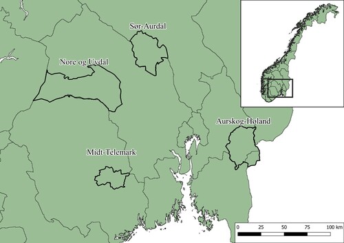
The average annual temperatures of the study areas range from 0 to 6°C. The topography of Norway features jagged mountains and deep valleys, and this was reflected in most of the study area. The sampled forests ranged from areas in close proximity to the tree line to lowland forests. Aurskog-Høland can, however, be regarded as more homogenous overall compared to the other municipalities, as the terrain is substantially flatter. In addition, it is the municipality with the strongest impact from forest harvest. “Bilberry woodlands” (Vaccinium myrtillus) and “Bilberry-lingonberry woodlands” (Vaccinium myrtillus-Vaccinium vitis-idaea) were the most frequent category of vegetation types (Larsson 2000).

Study design and sample tree selection

Several terms, such as veteran, ancient, heritage trees and champion trees, can overlap with the old tree, but these also emphasize other features than age. A veteran tree refers to a large tree with hollow trunks and receding crowns. An ancient tree is an old tree with veteran traits. Heritage and champions trees are mainly classified based on their cultural significance or size, respectively. Except for the term ancient, none of these related terms directly state that the trees must be old. For a more thorough discussion on these terms, see (Nolan et al. 2020). In our study, “Old tree” refers to a species-specific age threshold, i.e. Norway spruce trees older than 150 years and Scots pine older than 200 years (Baumann et al. 2001).

The fieldwork was carried out over two field seasons: Nore og Uvdal and Aurskog-Høland in August–October 2018 and Sør-Aurdal and Sauherad in August–September 2019. In each of the four municipalities, 10 old-tree habitats were selected randomly from the CHI registry (Anonymous 2021). Circular study-plots of 0.162 ha were laid out at the center of the old-tree habitats. The five in total assumed oldest living Norway spruce or Scots pine trees were carefully chosen within the study-plot following the CHI field guide’s descriptions. GPS coordinates were collected for each sample tree. The study-plot size and the selected number of sample trees corresponded to the minimum density threshold for the delimitation of old-tree habitats, i.e. at least three old trees per 0.1 ha (Baumann et al. 2001).

For each study-plot, a reference plot was established outside the respective Old-tree habitat. The purpose of the reference plots was to obtain similar tree age data from the oldest trees within a forest stand with comparable forest conditions in the vicinity of each of the Old-tree habitats. Two primary criteria were used to classify the reference plots. Firstly, they belonged to a mature forest cutting class V, i.e. forest old enough for harvest by foresters and located within 200–500 m from the Old-tree habitats. Secondly, the reference plots had the same elevation and composition of the main tree species. In one instance, an Old-tree habitat plot had no mature forest in the immediate vicinity. In this case, a reference plot was selected from the highest cutting class present (cutting class IV)

The paired-plot combination of study- and reference plots is referred to collectively as a locality. In total, 40 localities were selected, and consequently, 80 plots were included.

Site characteristics

The basal area (m² ha⁻¹) around each sample tree was measured with a relascope. The vertical forest structure and vegetation type (Larsson 2000) were classified within a 7-m radius of each sample tree. Vertical forest structure was divided into three categories: one-storied, two-storied or multistoried, based on trees’ representation in different canopy layers. An assessment of the topography within each study-plot was recorded in the following set of categories; (1) hilltop, (2) south-facing hill, (3) north-facing hill and (4) flat terrain (Table 1).

Table 1. A full list of all the collected variables, along with descriptive statistics for the Norway spruce sample trees.

Variable	Spruce – old-tree habitats		Spruce – references
	Mean	Range	Mean	Range
Tree variables
Age (years)	192.3	70–313	167.4	52–317
Height (m)	19.2	8.5–31.6	18.8	8.2–30.4
Diameter at 1.3 m (cm)	32.6	13.0–65.0	29.7	16.0–57
Diameter Height: ratio	1.7	1.1–3.6	1.6	0.9–4.5
Live crown (%)	80.6	53.7–99.3	77.5	29.2–100
Crown shape	2.6	1–4	2.6	1–4
Rot		0–1		0–1
Stem taper (%)	4.7	−0.74 to 12.3	6.1	0–16
Bark structure	3.0	1–4	2.6	1–4
Bark color	2.8	2–4	2.7	1–4
Spiral grain		0–1		0–1
Branch thickness (cm)	2.8	0–9	3.2	0–11
Drooping branches		0–1		0–1
Crookedness	2.0	1–4	1.8	1–4
Broken top/spike knot		0–1		0–1
Forked stems		1–2		1–2
Visible wounds		0–1		0–1
Site variables
Basal area (m^2 ha^−1)	19.4	5–45	21.9	4–50
Vertical forest structure		One – multistoried		One – multistoried
Vegetation type		Lichen – Tall herb		Lichen – Tall herb
Site index (m)	10.3	6–17	9.8	6–17
Topographic position	2.5	1–4	2.6	1–4
Distance to road (m)	650.2	46.3–1657.8	505.6	51.1–1726.7
Elevation (m)	650.0	207.9–1034.1	679.4	188.7–1018
Slope (%)	27.1	3.2–82.9	19.4	2.9–60.4

Note: The summary statistics is presented separately for each plot type.

Other site characteristics were based on geographic features and forest productivity measures analyzed in QGIS (QGIS Geographic Information System 2020). The K-nearest neighbors algorithm provided data on the proximity of forest access roads suited for timber harvests. Digital terrain models enabled the collection of elevation data in meters and the percentage slope of the 10-m radius buffer area surrounding each sample tree. Forest stand productivity was supplied by site indexes from forest inventory maps. In this case, the H40 index was adopted, which is based on the dominating tree species height at 40 years (Tveite and Braastad 1984). The forest inventory data was also collected from kilden.nibio.no (Anonymous 2021) and access road datasets from “vbase”. Data for DTM 10 were compiled from the geonorge.no database which is hosted at the Norwegian Map Authority (The Norwegian Mapping Authority 2021).

Morphological tree variables

Morphological traits reflecting size and shape were measured for every sample tree. Tree height in decimeters and the length of the living crown from the lowest living branch to the tree apex were measured with a vertex hypsometer. The relative crown length was calculated as the length of the living crown in percent of the total tree height. Cross calipered diameter at 1.3-m height (DBH) was measured to the nearest half-cm. Height and diameter registrations were combined into a diameter height ratio. Stem taper was estimated as the relative (%) change in diameter from breast height to the height of 5 m. The diameter at 5 m was estimated from photographs of trees, utilizing the known DBH (details in Appendix).

Different types of eccentricities along the tree stems were measured for each sample tree. The degree of stem crookedness was visually assessed as the deviation of the stem from a straight line, a leveled factor from 1 to 5 and devised from the lower ¾ of the tree stem. The scale measured the deviance from a straight line, and the classes were (1) < 2 cm, (2) 2–5 cm, (3) 6–15 cm, (4) 16–30 cm and (5) >30 cm. However, the crookedness also measured stem sinuosity. Trees with a strongly sinuous pattern were always classified as (>3) as they all were highly curved. Other registered eccentricities were the number of forked stems, the presence or absence of visible spike knots after a top breakage and the presence of wounding on the stem.

Additional species-specific morphological variables were defined to account for species-specific traits in pine and spruce trees (Table 2). Discriminant values of the different classes of bark texture, bark color, branch thickness and crown shape were defined and recorded. Initially, bark texture and bark color were encoded as five leveled factors, but this was simplified after the fieldwork to a four leveled factor because only two observations were found for the highest levels (Table 2). Spiral grain and drooping branches were recorded for both species, but since no spruce trees had visible spiral grain, and only one tree was without drooping branches, these parameters were only applicable for pine (Table 3).

Table 2. A full list of all the collected variables, along with descriptive statistics for the Scots pine sample trees.

Variable	Pine – old-tree habitats		Pine – references
	Mean	Range	Mean	Range
Tree variables
Age (years)	241.6	108–414	185.8	54–442
Height (m)	15.1	6.1–37.4	17.0	5.1–30.6
Diameter at 1.3 m (cm)	37.3	15.0–84	37.6	19.0–69
Diameter Height: ratio	2.8	1.1–9.6	2.4	0.8–5.4
Live crown (%)	43.0	6.2–84.4	77.5	29.2–100
Crown shape	2.3	1–4	1.7	1–4
Rot		0–1		0–1
Stem taper (%)	5.6	−1.8 to 21.4	5	−17.9 to 15.48
Bark structure	2.8	1–4	2.1	1–4
Bark color	3.1	1–5	3.0	1–5
Spiral grain		0–1		0–1
Branch thickness (cm)		0 to >20		0 to >20
Drooping branches		0–1		0–1
Crookedness	2.8	1–4	2.6	1–4
Broken top/spike knot		0–1		0–1
Forked stems		1–2		1–2
Visible wounds		0–1		0–1
Site variables
Basal area (m^2ha^−1)	19.1	5–36	21.9	4–50
Vertical forest structure		One – multistoried		One – multistoried
Vegetation type		Lichen – Tall herb		Bilberry-lingonberry – Tall herb
Site index (m)	9.5	6–17	10.3	6–17
Topographic position	2.1	1–4	2.1	1–4
Distance to road (m)	574.3	56.6–1396	433.0	51.1–1726.7
Elevation (m)	464.0	148.6–926.7	414.0	161–890
Slope (%)	23.8	3.2–82.9	23.8	1.3–84

The summary statistics are presented separately for each plot type.

Core extraction

The height of 0.5 m was chosen as the primary extraction point for core samples, whereas cores located at 1.3 m in height were also taken to achieve a better age estimate if butt rot was detected. The differences in coring height come as a compromise between ascertaining the total tree age while still being able to successfully extract a sample core. Often this was related to turning the handle of the corer or detecting butt rot within the sample core. Trees with rot were cored again at 1.3 m, and if rot was present on that core, this was also noted (Table 1).

Age determination of trees

Tree rings were measured using lintab 6 and the dendrochronology software TSAP-Win (Rinntech 2003). Incomplete core samples were corrected for the remaining distance to the pith. This was done by comparing the curvature of the last intact tree rings with a plastic template that had concentric circles (Applequist 1958). The distance to the pith was translated into an estimate of the remaining tree rings by dividing it with the mean width of the ten closest growth rings. Four of the trees had age corrections > 100 years, and these were capped at 100 years. Of the trees included in the sample, eight trees had more than 4 cm missing to the center of the pith. However, these were either characterized by large ring widths throughout their life or they were confirmed old trees by the total number of rings present already on the core. The number of growth rings in the samples was adjusted according to the core extraction height. One growth ring was added for every 5 cm in core extraction height above ground to provide an approximate for the true tree age (Kuuluvainen et al. 2002). Some core samples from Nore og Uvdal were unfortunately corrupted and were excluded from the material. This resulted in a total of 373 trees with estimates of total age that were included in the analysis.

Table 3. Species-specific tree variables.

Variable	Datatype	Norway spruce	Scots pine
Crown measurements	Ordered factor 1–4	Crown width: (1) > 0.7 m, (2) 0.7–1.5 m, (3) 1.5–4 m and (4) >4 m	Crown flatness was a measure of declining height growth with increasing age. (1) was cone-shaped, (2) strongly ellipsoid, (3) some curvature and (4) completely flat
Bark structure	Ordered factor 1–4	The bark thickness and roughness were expected to increase with age. The different bark morphologies were: (1) Smooth, (2) furrowed, (3) rough and (4) very rough.	This variable reflects the change from a cracked juvenile bark to a bark consisting of large, tightly interlocking plates: (1) Wide fissures, (2) fissured, (3) Bark plates and (4) dense plates.
Bark color	Ordered factor 1–4	A color variation on the first 5 meters of the stem from brown to increasingly light gray. These were brown, dark gray, gray and light gray.	Bark color variation on the first 5 m of the stem from orange to gray. (1) Orange, (2) dark brown, (3) brown gray and (4) gray
Branch thickness	Continuous/Ordered factor 1–4	The branch thickness was gathered by measuring the thickest branch in cm from within the stem’s lower 2.3 m.	The crown’s thickest branch was categorized into four levels: 0–5 cm, 6–10 cm, 11–20 cm and >20 cm.
Visible spiral grain	Binomial	Absent	Trees with visibly twisted right-oriented patterns on the stem were noted as spiral grained trees.
Drooping branches	Binomial	Only one found	To qualify as drooping branches, more than half of the branches on the tree inclined downwards.

Statistical analysis

To test the efficiency of the CHI method to visually identify patches of old trees, we compared age measurements of trees from Old-tree habitats to similar measurements from similar forest stands in the vicinity that were not recorded as Old-tree habitats. For this analysis, we used a pairwise t-test to test the difference in the mean age of the oldest trees on each plot pair (locality).

For the investigation of which tree variables and site characteristics that best function as indicators of old trees, we used regression models with tree age as a response and tree variables and site characteristics as dependent variables. All the analyses were performed in the statistical software R (R Core team 2018), and the presented figures were made using the package “ggplot2”.

Comparing the age of the oldest trees in the old-tree habitats with references

The Old-tree habitats and the reference plots were treated as pairs under the assumption that each locality, at some degree, shared a common forest history and site conditions. The mean age of the trees sampled in each study-plot was calculated. The mean plot age fulfilled the assumption of normality, and a pairwise t-test was deemed an appropriate test. We tested the null hypothesis that the mean of the age difference is equal. A complete list of the study-plot pairs containing the mean age of the oldest trees, locality number and the municipality is available in supplementary material 1.

Age regression models

The age models were constructed using a generalized linear mixed modeling approach to account for spatial autocorrelation between the sample trees within each of the localities (Crawley 2013). Localities and study-plots were represented in the models as random intercepts. The random effects structure was modeled by nesting each of the study-plot pairs by their locality. A random effect structure that also included municipality showed that the random effect variance from the municipality variable was exceedingly small (4.52 * 10⁻¹⁰), and thus this was left out from further analyses. The variation explained by the random clustering effect was measured through the intra-class correlation (ICC) (Crawley 2013). Continuous explanatory variables were centered and scaled to account for the large difference in scale between some variables.

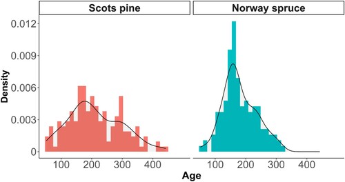
Both tree species featured skewed age distributions (Figure 2). To accommodate for positive and skewed values, we used a generalized linear mixed model with a gamma distribution (Crawley 2013). Generalized linear models provide flexibility in that they can account for error structures that are not normally distributed yet have a non-constant variance (Nelder and Wedderburn 1972). Age models were fitted with a log-link function by maximum likelihood in the package “glmmTMB” (Brooks et al. 2017). In this case, the age models were shown to all converge.

Figure 2. The age distributions in the sample represented as a combination between density plots and histogram with a bin width of 30 years

The models and their assumptions were described in the following way. (Notation from Nakagawa et al. 2017). The two sides of the equation $y_{ijk}=\mathrm{g}\mathrm{a}\mathrm{m}\mathrm{m}\mathrm{a}\left({\lambda }_{ijk},v\right)$

refers to; $y_{ijk}$, the ith observation/tree of the jth study-plot in the kth locality is defined by the two gamma-distributed parameters $\lambda$ and $v$. $v$ is the shape parameter of the distribution, while $\lambda$ is the mean of the gamma distribution, and the variance is ${\displaystyle \frac{{\lambda }^2}{v}}$. The expression $\ln \left({\lambda }_{ijk}\right)={\text{β}}_0+\sum _{h=1}^k{\text{β}}_h{x}_{h_{ij}k}+{\mathrm{{\rm Y}}}_k+{\alpha }_{jk}$

refers to the log-link function. $\ln \left({\lambda }_{ijk}\right)$ is the latent value for the ith tree of the jth study-plot in the kth locality. ${\mathrm{{\rm Y}}}_k\sim \mathrm{G}\mathrm{a}\mathrm{u}\mathrm{s}\mathrm{s}\mathrm{i}\mathrm{a}\mathrm{n}\left(0,{\sigma }_a^2\right)$

signifies each locality, which is assumed to be normal distributed around 0 with variance ${\sigma }_{\mathrm{{\rm Y}}}^2$. ${\alpha }_{jk}\sim \mathrm{G}\mathrm{a}\mathrm{u}\mathrm{s}\mathrm{s}\mathrm{i}\mathrm{a}\mathrm{n}\left(0,{\sigma }_a^2\right)$

refers to each study-plot pair which is nested inside each locality. This is assumed to be normally distributed around 0, with a variance of ${\sigma }_a^2$. The residual variance was approximated using the trigamma function: $e_{ijk}=\log \left(\psi \right)$

Model assumptions were tested with the package “DHARMa” which provides simulated residuals for generalized linear mixed models (Hartig 2020). The simulated residuals indicated that the gamma distribution was an appropriate fit for Norway spruce. The Scots pine models had a good fit, but these models were shown to underestimate the medium-aged trees’ age slightly, since bimodality was evident in the age distribution (Figure 2). Bimodality was, however, not caused by the differences between the study-plots in Old-tree habitats and/or reference plots (results not shown).

Effect size

Marginal R² and conditional R² determinations were extended into generalized linear mixed models with gamma as a measure of the goodness of fit (Nakagawa et al. 2013; Nakagawa et al. 2017). The marginal R² determination measures the variance explained by the fixed effects of the models, while the conditional R² included the random effect variance (Nakagawa et al. 2013). Supplying both determinations was seen as advantageous since they provided an intuitive comparison of both the fit from the explanatory models and then the relative contribution from random effects (Nakagawa et al. 2013; Nakagawa et al. 2017). Both R²s were calculated using the trigamma method in “r2.squared.glmm” from the package “MuMIn” (Nakagawa et al. 2017; Barton 2020).

Variable selection

Second-order terms were allowed in the models, and all variables were inspected for potential interactions. This inspection was related to the objective that interpretated the causal relationships between the variables. Kendall’s tau, a rank-based correlation coefficient, was used to look at relationships between categorical and continuous variables (supplementary material for full correlation matrix). In two cases, the interpretation of the relationships was problematic. Stem taper could not be calculated for all the trees, and thus analyses were made with and without this variable to compare the effect. The rot variable was also not included in the final models as it can only be found by coring, and thus, this did not align with the purpose of determining age visually.

Model selection

Model selection was made by comparing the AICc weight and residual analysis from different realistic models. The main aim was to find the most parsimonious models. Unless stated otherwise, the models shown in the results had an AICc weight >0.7. All the models were inspected for collinearity using generalized variance inflation and visual inspection by scatter plots.

Cross-validation

The robustness of the tree age models in terms of prediction was tested by cross-validation. A resampling procedure was repeated with 500 iterations for both tree species to estimate the bias of the estimator and the corresponding standard error. The prediction models were refitted on a fixed number of resampled trees randomly selected for each iteration. For each iteration, the refitted models were used to predict the age of the sample trees left for validation, and the mean difference between the measured tree ages and the predicted ages was calculated. The standard error of the overall mean difference was estimated as the standard deviation of the 500 individual mean differences. The Scots pine model was fit with 160 sample trees and validated on the remaining 31 sample trees. Similarly, the Norway spruce model was fit with 120 sample trees and validated on 20 sample trees.

Results

Comparing the age of the oldest trees in the old-tree habitats with references

The mean age of the trees in the Old-tree habitats was significantly older than those in the reference plots. The age differences between the plots were, on average, 41.9 years (p-value > 0.001, 38 pairs, CI (24.9, 61.6), Figure 3). A general trend was that localities with a high mean age in the Old-tree habitats had reference plots with correspondingly old trees (Simple linear R² = 0.21, p-value > 0.005). Of the 38 pairs, seven had reference plots with higher mean age compared to the Old-tree habitats. These seven discrepancies still fulfilled the age requirements (200 for Scots pine and 150 for Norway spruce) defined for the given tree species. However, there were some indications that pine-dominated Old-tree habitats were more clearly differentiated than the spruce-dominated ones (Table 2).

Age regression models

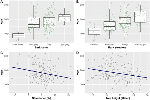
The measured morphological variables explained more age variance than the site variables, and the Scots pine models showed stronger relationships than the Norway spruce models. The age models for the two species were markedly different (Tables 4 and 5 and Figures 4 and 5). Several species-specific morphological traits were prominent in the models. Importantly no positive relation between age and large size was found. Instead, a negative correlation with tree height was identified. The majority of the oldest trees were not tall, and this was especially evident for Scots pine, where none of the trees older than 300 years stood taller than 20 m.

Figure 3. Boxplot comparison of the mean age of the oldest trees on each plot where the line shown in each box is the median age. The observations have been jittered using a width of 0.37 in the geom_jitter() function in ggplot2 to avoid overplotting.

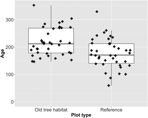
Figure 4. All the variables are included in the best model. Scots pine model excluding drooping branches. Categorical variables are shown as boxplots with jittering of the observations to avoid overplotting. Continuous variables are shown as scatterplots.

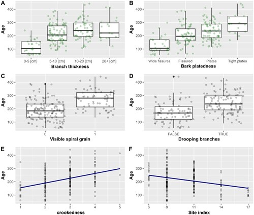
Table 4. The selected Scots pine model.

Age model Scots pine
Fixed effects	Estimate	SE	z Value	Pr(>|z|)
(Intercept)	4.586	0.085	53.87	***
Bark structure [2]	0.197	0.056	3.48	***
Bark structure [3]	0.277	0.065	4.23	***
Bark structure [4]	0.518	0.090	5.76	***
Visible spiral grain	0.128	0.042	3.06	**
Branch thickness [2]	0.186	0.060	3.08	**
Branch thickness [3]	0.263	0.070	3.76	***
Branch thickness [4]	0.263	0.083	3.19	**
Crookedness	0.071	0.021	3.41	***
Drooping branches	0.119	0.039	3.02	**
Scaled (Site index)	−0.094	0.031	−3.09	**
Random effects
ICC	0.53	–	–	–
NLocalities	27	–	–	–
Nplots	53	–	–	–
Observations	191	–	–	–
Marginal $R_{\mathrm{g}\mathrm{a}\mathrm{m}\mathrm{m}\mathrm{a}}^2$	0.51	–	–	–
Conditional $R_{\mathrm{g}\mathrm{a}\mathrm{m}\mathrm{m}\mathrm{a}}^2$	0.77	–	–	–

Notes: Bark structure, visible spiral grain and branch thickness are represented in the model as dummy variables, while site index and crookedness are continuous. ns corresponds to non-significant, *, ** and *** corresponds to p-values of >0.05 (non-significant), <0.05 and <0.

Table 5. The selected Norway spruce model.

Age model Scots pine
Fixed effects	Estimate	SE	z value	Pr(>|z|)
(Intercept)	4.369	0.161	27.18	***
Bark structure [2]	0.635	0.217	2.93	**
Bark structure [3]	0.646	0.212	3.04	**
Bark structure [4]	0.782	0.225	3.48	***
Branch color [2]	0.077	0.146	0.53	ns
Branch color [3]	0.166	0.144	1.15	ns
Branch color [4]	0.329	0.150	2.19	*
Scaled (Stem taper)	−0.076	0.021	−3.71	***
Scaled (Height)	−0.067	0.025	−2.69	**
Scaled(Stem taper) * Scaled (Height)	−0.062	0.023	−2.75	**
Random effects
ICC	0.14	–	–	–
NLocalities	22	–	–	–
Nplots	40	–	–	–
Observations	191	–	–	–
Marginal $R_{\mathrm{g}\mathrm{a}\mathrm{m}\mathrm{m}\mathrm{a}}^2$	0.40	–	–	–
Conditional $R_{\mathrm{g}\mathrm{a}\mathrm{m}\mathrm{m}\mathrm{a}}^2$	0.47	–	–	–

Notes: Bark roughness and Bark color are represented in the model as dummy variables, while Stem taper and Height are continuous. ns, *, ** and *** corresponds to p-values that are >0.05 (non-significant), <0.05, <0.01 and 0.001.

Including site variables in addition to morphological variables did not provide additional explanatory power, except when the productivity variable site index (H40) was included. Most productivity measures were, however, weakly linked with age (Kendall correlation coefficient τ < 0.22). The only multicollinearity was observed between the H40 site index and with the elevation data for Norway spruce. This had a Kendall correlation coefficient of τ = 0.63.

Scots pine

Age models for Scots pine performed better than for Norway spruce. However, Scots pine models also had the largest random effect term (n = 192, Marginal $R_{\mathrm{g}\mathrm{a}\mathrm{m}\mathrm{m}\mathrm{a}}^2$ = 0.51, Conditional $R_{\mathrm{g}\mathrm{a}\mathrm{m}\mathrm{m}\mathrm{a}}^2$ = 0.77). The oldest Scots pine trees were characterized by densely spaced bark plates, drooping branches, visible spiral grain and the selected model also included the H40 site index. The same model (Table 4), when height included, was similar (AICc weight = 0.655). Diameter at breast height and age were positively correlated, but the diameter was excluded from the final selected model.

Norway spruce

The selected Norway spruce model moderately explained the age variance (n = 139, Marginal $R_{\mathrm{g}\mathrm{a}\mathrm{m}\mathrm{m}\mathrm{a}}^2$ = 0.40, Conditional $R_{\mathrm{g}\mathrm{a}\mathrm{m}\mathrm{m}\mathrm{a}}^2$ = 0.47). The oldest spruce trees were characterized by light gray rough bark and columnar stems. The best model, when considered without the stem taper variable, and which included all the spruce tree samples, was, however, substantially weaker (n = 183, Marginal $R_{\mathrm{g}\mathrm{a}\mathrm{m}\mathrm{m}\mathrm{a}}^2$= 0.26, Conditional $R_{\mathrm{g}\mathrm{a}\mathrm{m}\mathrm{m}\mathrm{a}}^2$= 0.34). Site index was also shown to correlate with tree height. A comparison with a model where the same variables were considered but where the site index was included instead of tree height showed a highly similar fit (AICc weight = 0.63).

Cross-validation

The models only featured a minor bias. The result of the cross-validation with 500 resampling runs led to a bias of −5.4 with a standard deviation of 10.9 for Scots pine. Norway spruce had a bias of −1.6 with a standard deviation of 11.9.

Discussion

The oldest trees in the Old-tree habitats, identified visually using morphological traits, were on average 41.9 years older than comparable mature forests. Age regression models based on morphological and site characteristics explained around half of the age variation, and they performed better for Scots pine than for Norway spruce. Furthermore, the results show that visual age determination of Norway spruce and Scots pine benefitted from the inclusion of several discrete morphological characteristics used in a combination.

Most Old-tree habitats in this study included trees with total age estimates older than the defined age limits of 150 and 200 years (Baumann et al. 2001) for Norway spruce and Scots pine, respectively. Additionally, several of the reference plots had estimated ages well above these limits (Figure 3). The registration of Old-tree habitats requires a density corresponding to >30 old trees ha⁻¹ on a minimum of 0.2 ha to be mapped (Baumann et al. 2001). Given the size of the study-plots (0.162 ha), these reference plots would be eligible as Old-tree habitats. Some of these reference plots may indeed represent potential Old-tree habitats that border the requirements in registration or are overlooked by the forest planners during the survey. Nevertheless, applying the visual method did succeed in finding areas with old trees present.

Visual identification of old trees is not a measure without error (Pederson 2010; Brown et al. 2019). To determine the age of old trees using visual traits can be difficult and requires experience. Extra information gathered from the field may aid the process of selecting which areas to set aside. In this sense, photographs and rough classification of the tree ages can serve as additional documentation to later help the selection process. Likewise, the knowledge gained from this study may also likely reduce the future error rate. However, it is important to acknowledge that some old trees will remain undiscovered and similarly, some younger trees will also be falsely registered as old trees.

Forest history and current developments also affect the area, which can be eligible as Old-tree habitats. It is expected that there would be old trees outside the areas delimited by the forest planners as nearby localities tend to share general forest conditions. Because the amount of old forest in Norway is increasing, some areas adjacent to the Old-tree habitats now may meet the age requirements. Nevertheless, untangling which reference plots that could qualify as Old-tree habitats or were marginally classified as those habitats, was deemed outside the scope of this study since comparisons were only made between the ages of the paired study and reference plots.

Areas with old Scots pine trees were identified with more certainty compared to their spruce counterparts. Firstly, this may be because they have wider age demography than Norway spruce. Secondly, spruce forests are often darker and dense, making it harder to assess the older trees. Lastly, but perhaps the most important reason according to the age regression models: Scots pine trees have several better performing characteristics that correlate with age. When these factors are taken together, old Scots pine trees were easier to identify when compared to the variation observed in Norway spruce trees.

Of the site characteristics, the H40 site index contributed the most to tree age prediction. Although the maximum age of pines to some degree seems to be explained by aspect and slope (Bigler and Zang 2016), for spruce and pine trees as a whole, site characteristics are shown to be weak predictors of age (Bigler and Veblen 2009; Rötheli et al. 2012; Castagneri et al. 2013). Nevertheless, the site index parameter appears to be easiest to utilize as it both directly summarizes the various site conditions which regulate tree growth, and in many cases, can readily be accessed from forest resource maps (Sharma et al. 2012). This index can also be used to distinguish between medium-aged trees and old trees of the same size (Alberdi et al. 2013; Brown et al. 2019).

Site index and tree height were confounded (Supplementary) but seemed to diverge in older trees. The site index values are based on the height of the dominating trees (Tveite and Braastad 1984). Thus, in low productivity localities, one would expect shorter trees at a given age and lower potential maximum heights. Moreover, the oldest trees in the stand and the dominating trees are also not necessarily the same. The oldest trees measured in the current study were not the tallest. This may be because the utilized site indexes were initially developed for even-aged production forests, and old trees exceed the forest management cycles. Additionally, the age of the trees used to measure site index is also underestimated if they have been suppressed by neighboring trees in the past. In other words, site indexes aim to indicate site productivity and not age, but they can likely provide indications on the whereabouts of old trees.

The potential difference between the dominating trees and the oldest trees can be illustrated with two alternative life-history strategies; grow fast or grow slow (Bigler and Zang 2016). The first of these results in a competitive advantage early and while the latter increases the time available to reproduce. Slow growth seems to be a prerequisite for longevity (Black et al. 2008; Castagneri et al. 2013). Moreover, longer exposure times can increase the likelihood of treetop breakage (Kuuluvainen et al. 2002). Together these two factors can make tree height an unreliable indicator of age.

Old Scots pine trees often featured distinctive crowns, crooked stems and closely spaced bark plates. Younger individuals tended to have thin branches facing upwards and fissured bark. Such a morphology indicates that the trees in question are still vigorously growing and have not yet developed the individual traits associated with old pines (Weisberg and Ko 2012; Brown et al. 2019). Furthermore, the crooked stems may indicate selection from former harvesting periods that avoided trees with poor timber quality. Nevertheless, most of the characteristic morphological traits likely result from the legacy of a long life.

The spiral grain pattern may reflect a life-history strategy that contributes to longevity in conifers. Spiral grain is a biological phenomenon in which the orientation of the outer wood forms a helical pattern (Kubler 1991). This pattern becomes stronger with age and is hypothesized to either stabilize the trees against the wind (Skatter and Kučera 1997) or increase drought resistance by spreading the water into a larger part of the crown (Kubler 1991). Thus, spiral grain may prove an advantageous trait for pine trees and improve their ability to grow old.

Old Norway spruce trees were identified by their rough and light-colored gray bark. The properties of the bark are known to change with increasing age. However, age-related bark characteristics appear less prominent in spruces than pines (Van Pelt 2007; Pederson 2010; Weisberg and Ko 2012). The age varied considerably in Norway spruce trees, even when these trees had similar bark features. Bark color was the most statistically significant of the two bark variables, although bark color was prone to change with moisture content (own observation). When bark color was left out of the models (results not shown), the bark structure variable increased in statistical significance. Therefore, bark structure may serve an important role in identifying old individuals.

The stems of Norway spruce trees became less tapered with age. Juvenile trees generally tend to increase the stem diameter on the lower parts of the stem, but this difference evened out with increasing age. Thus, older trees usually have less tapered stems (Pederson 2010). However, some spruce trees are known to develop large root buttresses (Van Pelt 2007). Root buttresses were accounted for by calculating the stem taper between 1.3 and 5 m in tree height. Still, stem taper was not found independent of tree size, but this was adjusted for with an interaction term. Tapering was shown to be less in tall trees, but there are uncertainties as to how vital this interaction is for practical registration.

It seems that old age morphology is more distinct in old pine trees than old spruces (Rötheli et al. 2012; Weisberg and Ko 2012). Individual traits such as bark structure appear to be more distinctively associated with age for pine trees compared to that of spruce trees. With age, pines accumulate significant crown dieback leading to shorter, more open crowns (Weisberg and Ko 2012). This openness also makes it easier to assess other old age indicators as one gets a better view of the stem and the individual branches. In comparison, spruces show less variation with age in the bark and may retain their symmetric crowns for 200–300 years (Van Pelt 2007). Consequently, investigating other age indicators may improve the discovery of older spruces. One such alternative may be the presence or absence of visible scars from branches on the bole directly underneath the crown.

Remarkably, the age variation explained by the random effects for Scots pine was considerable, meaning that tree ages from each plot were more homogenous than that of Norway spruce. The substantial random effect for Scots pine trees may reflect their regeneration strategy. Scots pine predominantly regenerates in patches, whereas Norway spruce often regenerate by small-scale gap dynamics (Kuuluvainen and Aakala 2011). On a scale of 0.2 hectares, more Scots pine trees will belong to the same cohort. As a practical result, for this species, a single core sample using traditional age determination may also give relevant information on the age of surrounding trees.

The selected age regression models did not depend strongly on tree size. While the relationship between age and size in old trees is generally acknowledged to be weak (Kuuluvainen et al. 2002; Castagneri et al. 2013; Brown et al. 2019), it was still surprising how weak the relationship in our study was. This can be lingering effects from former periodical harvests selecting and removing the best and largest trees from the stand. The historic forest use in Norway is spatially extensive and difficult to disentangle from this dataset. While we cannot state for certain, we believe that the weak age-size relationship is inherently weaker in old trees. Sampling more young trees would likely reveal a monotonic positive relationship between age and size (Kuuluvainen et al. 2002; Castagneri et al. 2013). However, in old trees, the relation between size and age becomes weak due to a plateau effect. Once past 150–250 years old and depending on the site conditions, size seems to offer little information on the age for Norway spruce and Scots pine (Kuuluvainen et al. 2002; Brown et al. 2019).

The age regression models are explanatory but have generalizable results. The selected models maximize the explained age variation within the study area and are not directly aimed at prediction. Nevertheless, the sampling captures a wide environmental gradient, which might explain the low bias for the models. In addition, the mixed-effects models reduce overfitting by shrinking the random effect of locality (Crawley 2013). We deem that the currently devised models would translate to various forest types, including those with old characteristics.

Similar to our methods, comparable approaches have been successfully applied in a range of forest types, including those from ancient trees on near untouched cliffs (Matthes et al. 2008), montane areas (Brown et al. 2019) and arid environments (Weisberg and Ko 2012). It is uncertain how well our models would work in different types of natural forests, but the tree ages in the sample are arguably comparable to old trees present in old boreal forests (Kuuluvainen et al. 2002). Recognizing old trees visually may serve as a useful component in locating or circumscribing remnants of old forests.

Figure 5. All the variables included in the best model exclude the interaction between stem taper and height. Categorical variables are shown as boxplots with jittering of the observations to avoid overplotting. Continuous variables are shown as scatterplots.

Conclusion

This is the first comprehensive study of visual morphological traits that indicate old age in Norway spruce and Scots pine trees. We found several characteristics such as bark texture, stem taper and visible growth eccentricities that can be used to obtain age estimates for old trees. For Norway spruce, the models indicate that the tapering at the lower stem, and the bark structure and color, are the most important visual morphological traits for finding the oldest individuals. Determining the age of Scots pine visually benefits from assessing the whole tree, where characteristics like bark plates, branch morphology and stem eccentricities seem to be the most influential. For both species, a low site index may increase the probability of finding the old trees.

If the goal is to preserve or manage old trees within the forest matrix, one needs information about their whereabouts. Old trees represent habitats that require centuries to accumulate. Unlike dead wood such as logs and snags, one cannot simply make old trees, as they are unavoidably bound with time. Finding the old trees within the forest landscape is therefore vital to aid management decisions.

Acknowledgments

The authors thank Kajsa Sivertsen and Alexander Saša Bjelanović for their assistance with the fieldwork, and Adam Vivian-Smith and Wibecke Nordstrøm for proofreading the manuscript. We are also grateful to the reviewers for their valuable input, which considerably improved the manuscript.

Disclosure statement

No potential competing interest was reported by the authors.

Data availability

The data that support the findings of this study are available from the corresponding author, E.H., upon reasonable request.

Additional information

Funding

This work was supported by Norwegian Ministry of Agriculture and Food.

Appendix

Stem taper (%) was calculated from photographs as the difference between the diameter at 1.3 m and the diameter at 5-m height. These heights were chosen to enable a standardized comparison of the stem taper trees of varying tree heights and avoid the extreme stem taper in the lower part of the stem. Colored bands were tied around 1.3 m to locate the sample trees and connect the photographs with the field measurements. We translated the known field measurements into pixels for each sample tree. Therefore, we could use the ratio between the field measurements and the pixels to locate the height and diameter of 5 m on the stem. The difference in size at 5 m caused by the increased distance was adjusted with trigonometry. A triangle was calculated with the distance to the sample tree as length and 5 m as height. The diameter at 5 m height on the tree was corrected with the difference between the hypotenuse and length of the triangle.

References

- Alberdi I, Cañellas I, Hernández L, Condés S. 2013. A new method for the identification of old-growth trees in national forest inventories: application to Pinus halepensis mill. stands in Spain. Ann For Sci. 70(3):277–285.
- Andersson J, Domingo Gómez E, Michon S, Roberge J-M. 2018. Tree cavity densities and characteristics in managed and unmanaged Swedish boreal forest. Scand J For Res. 33(3):233–244.
- Andersson R, Östlund L. 2004. Spatial patterns, density changes and implications on biodiversity for old trees in the boreal landscape of northern Sweden. Biol Conserv. 118(4):443–453.
- Anonymous. 2021. Kilden – Arealinformasjon. Kilden: NIBIO.
- Applequist MB. 1958. A simple pith locator for use with off-center increment cores. J For. 56(2):141.
- Barton K. 2020. Package “MuMIn”: Multi-Model Inference.
- Baumann C, Gjerde I, Blom HH, Sætersdal M, Nilsen JE, Løken B, Ekanger I. 2001. Miljøregistrering i skog – Biologisk mangfold. Håndbok i registrering av livsmiljøer i skog. Hefte 3. Instruks for registrering 2001: Bd. H. 3. Skogforsk.
- Bigler C, Veblen TT. 2009. Increased early growth rates decrease longevities of conifers in subalpine forests. Oikos. 118(8):1130–1138.
- Bigler C, Zang RG. 2016. Trade-offs between growth rate, tree size and lifespan of Mountain Pine (Pinus montana) in the Swiss National Park. PLoS ONE. 11(3):1–18.
- Black BA, Colbert JJ, Pederson N. 2008. Relationships between radial growth rates and lifespan within North American tree species. Écoscience. 15(3):349–357.
- Braun DC, Reynolds JD. 2012. Cost-effective variable selection in habitat surveys. Methods Eco Evol. 3(2):388–396.
- Brooks ME, Kristensen K, van Benthem KJ, Magnusson A, Berg CW, Nielsen A, Skaug HJ, Mächler M, Bolker BM. 2017. GlmmTMB balances speed and flexibility among packages for zero-inflated generalized linear mixed modeling. R J. 9(2):378–400.
- Brown PM, Gannon B, Battaglia MA, Fornwalt PJ, Huckaby LS, Cheng AS, Baggett LS. 2019. Identifying old trees to inform ecological restoration in montane forests of the central Rocky Mountains, USA. Tree-Ring Res. 75(1):34–48.
- Castagneri D, Storaunet KO, Rolstad J. 2013. Age and growth patterns of old Norway spruce trees in Trillemarka forest, Norway. Scand J For Res. 28:232–240.
- Crawley MJ. 2013. The R book. 2nd ed. Hoboken (NJ): Wiley.
- Gauthier S, Bernier P, Kuuluvainen T, Shvidenko AZ, Schepaschenko DG. 2015. Boreal forest health and global change. Science. 349(6250):819–822.
- Gjerde I, Sætersdal M, Blom HH. 2007. Complementary Hotspot Inventory – a method for identification of important areas for biodiversity at the forest stand level. Biol Conserv. 137(4):549–557.
- Grantham HS, Moilanen A, Wilson KA, Pressey RL, Rebelo TG, Possingham HP. 2008. Diminishing return on investment for biodiversity data in conservation planning. Conserv Lett. 1:190–198.
- Handegard E. 2020. Identifying old Norway spruce and Scots pine trees by visual inspection: an analysis of the relationship between age, spatial distribution and morphological traits in trees [Norwegian University of Life Sciences]. https://hdl.handle.net/11250/2679452.
- Hartig F. 2020. DHARMa: residual diagnostics for hierarchical (multi-level/mixed) regression models. https://CRAN.R-project.org/package=DHARMa.
- Henttonen HM, Nöjd P, Suvanto S, Heikkinen J, Mäkinen H. 2019. Large trees have increased greatly in Finland during 1921–2013, but recent observations on old trees tell a different story. Ecol Indic. 99:118–129.
- Kirby K, Watkins C. 2015. Europe’s changing woods and forests: from wildwood to managed landscapes. Wallingford: CABI Publishing.
- Kubler H. 1991. Function of spiral grain in trees. Trees. 5(3):125–135.
- Kuuluvainen T, Aakala T. 2011. Natural forest dynamics in boreal fennoscandia: a review and classification. Silva Fenn. 45(5):823–841.
- Kuuluvainen T, Gauthier S. 2018. Young and old forest in the boreal: critical stages of ecosystem dynamics and management under global change. For Ecosyst. 5(1):26.
- Kuuluvainen Timo, Mäki Juha, Karjalainen Leena, Lehtonen Hannu. 2002. Tree age distributions in old-growth forest sites in Vienansalo wilderness, eastern Fennoscandia. Silva Fennica. 36(1). https://doi.org/http://doi.org/10.14214/sf.556.
- Larsson John Y. 2000. Veiledning i bestemmelse av vegetasjonstyper i skog. Ås: Norsk institutt for jord- og skogkartlegging.
- Lie MH, Arup U, Grytnes JA, Ohlson M. 2009. The importance of host tree age, size and growth rate as determinants of epiphytic lichen diversity in boreal spruce forests. Biodivers Conserv. 18(13):3579–3596.
- Lindenmayer D, Franklin J. 2002. Conserving forest biodiversity: a comprehensive multiscaled approach. Washington (DC): Island Press.
- Lindenmayer DB, Laurance WF, Franklin JF, Likens GE, Banks SC, Blanchard W, Gibbons P, Ikin K, Blair D, Mcburney L, et al. 2014. New policies for old trees: averting a global crisis in a keystone ecological structure. Conserv Lett. 7(1):61–69.
- Linder P, Östlund L. 1998. Structural changes in three mid-boreal Swedish forest landscapes, 1885-1996. Biol Conserv. 85:9–19.
- Liu J, Yang B, Lindenmayer DB. 2019. The oldest trees in China and where to find them. Front Ecol Environ. 17(6):319–322.
- Matthes U, Kelly PE, Larson DW. 2008. Predicting the age of ancient Thuja occidentalis on cliffs. Can J For Res. 38(12):2923–2931.
- Naidoo R, Balmford A, Ferraro PJ, Polasky S, Ricketts TH, Rouget M. 2006. Integrating economic costs into conservation planning. Trends Ecol Evol. 21(12):681–687.
- Nakagawa S, Johnson PCD, Schielzeth H. 2017. The coefficient of determination R2 and intra-class correlation coefficient from generalized linear mixed-effects models revisited and expanded. J R Soc Interface. 14(134):20170213.
- Nakagawa S, Schielzeth H, O'Hara RB. 2013. A general and simple method for obtaining R2 from generalized linear mixed-effects models. Methods Ecol Evol. 4(2):133–142.
- Nascimbene J, Marini L, Motta R, Nimis PL. 2009. Influence of tree age, tree size and crown structure on lichen communities in mature Alpine spruce forests. Biodivers Conserv. 18(6):1509–1522.
- Nelder JA, Wedderburn RWM. 1972. Generalized linear models. J Royal Stat Soc Ser A (Gen). 135(3):370. https://doi.org/https://doi.org/10.2307/2344614.
- Nolan V, Reader T, Gilbert F, Atkinson N. 2020. The ancient tree inventory: a summary of the results of a 15 year citizen science project recording ancient, veteran and notable trees across the UK. Biodivers Conserv. 29(11):3103–3129.
- Pederson N. 2010. External characteristics of old trees in the eastern deciduous forest. Nat Areas J. 30:396–407.
- QGIS Geographic Information System (3.2.3). 2020. Open Source Geospatial Foundation Project.
- R Core team. 2018. A language and environment for statistical computing. Vienna: R Foundation for Statistical Computing.
- Rinntech. 2003. TSAP-Win User Reference (version 0.53).
- Rötheli E, Heiri C, Bigler C. 2012. Effects of growth rates, tree morphology and site conditions on longevity of Norway spruce in the northern Swiss Alps. Eur J For Res. 131(4):1117–1125.
- Sharma RP, Brunner A, Eid T. 2012. Site index prediction from site and climate variables for Norway spruce and Scots pine in Norway. Scand J For Res. 27(7):619–636.
- Skatter S, Kučera B. 1997. Spiral grain – an adaptation of trees to withstand stem breakage caused by wind-induced torsion. Eur J Wood Wood Prod. 55(4):207–213.
- Sætersdal M, Gjerde I, Heegaard E, Schei F, Nilsen J. 2016. History and productivity determine the spatial distribution of key habitats for biodiversity in Norwegian forest landscapes. Forests. 7(12):11.
- The Norwegian Mapping Authority. 2021. Geonorge. https://www.geonorge.no/.
- Thunes KH, Skarveit J, Gjerde I. 2003. The canopy arthropods of old and mature pine Pinus sylvestris in Norway. Ecography. 26(4):490–502.
- Tveite B, Braastad H. 1984. Bonitering for gran, furu og bjørk. Ås: Norsk institutt for skogforskning.
- Van Pelt R. 2007. Identifying mature and old forests in western Washington. I Washington State Department of Natural Resources (s. 1–104). https://www.dnr.wa.gov/publications/lm_hcp_west_oldgrowth_guide_full_lowres.pdf?u29mn4.
- Weisberg PJ, Ko DW. 2012. Old tree morphology in singleleaf pinyon pine (Pinus monophylla). For Ecol Manag. 263:67–73.
- Wetherbee R, Birkemoe T, Sverdrup-Thygeson A. 2020. Veteran trees are a source of natural enemies. Sci Rep. 10(1):18485.