Modelling height in adolescence: a comparison of methods for estimating the age at peak height velocity

Abstract

Background: Controlling for maturational status and timing is crucial in lifecourse epidemiology. One popular non-invasive measure of maturity is the age at peak height velocity (PHV). There are several ways to estimate age at PHV, but it is unclear which of these to use in practice.

Aim: To find the optimal approach for estimating age at PHV.

Subjects and methods: Methods included the Preece & Baines non-linear growth model, multi-level models with fractional polynomials, SuperImposition by Translation And Rotation (SITAR) and functional data analysis. These were compared through a simulation study and using data from a large cohort of adolescent boys from the Christ’s Hospital School.

Results: The SITAR model gave close to unbiased estimates of age at PHV, but convergence issues arose when measurement error was large. Preece & Baines achieved close to unbiased estimates, but shares similarity with the data generation model for our simulation study and was also computationally inefficient, taking 24 hours to fit the data from Christ’s Hospital School. Functional data analysis consistently converged, but had higher mean bias than SITAR. Almost all methods demonstrated strong correlations (r > 0.9) between true and estimated age at PHV.

Conclusions: Both SITAR or the PBGM are useful models for adolescent growth and provide unbiased estimates of age at peak height velocity. Care should be taken as substantial bias and variance can occur with large measurement error.

Keywords:

• Age at peak height velocity
• derivative estimation
• physical development
• lifecourse epidemiology
• pubertal timing

Introduction

Adolescence is, after infancy, the period of greatest change in our body composition and underlying biology (Viner et al., 2015). Studies of adolescent health are, therefore, crucial to the developmental origins of health and disease. A key requirement of any such study will be to account for maturational status and the timing of puberty. The age of peak height velocity (PHV) is often thought of as the gold standard of non-invasive measures of maturational status in observational studies. Age at PHV has been widely used as an outcome (Didcock et al., 1995; Mason et al., 2011; Nielsen, 1985; Price et al., 1988), exposure of interest (Gastin et al., 2013; Mao et al., 2013; Sherar et al., 2007), or as a covariate to control for confounding (Baxter-Jones et al., 2011; Darelid et al., 2012; Forwood et al., 2004). The appeal of age at PHV is twofold: (1) it applies equally to both boys and girls (Sherar et al., 2004); and (2) the measure appears to be objective, particularly in comparison to other methods that rely on subjective decisions about physical development of primary (Taranger et al., 1976) (orchoidometry) and secondary sex characteristics (Tanner, 1962) (Tanner Staging), recall of (semi-) specific biological events (age at menarche (Bergsten-Brucefors, 1976; Damon & Bajema, 1974; Damon et al., 1969)/voice breaking (Billewicz et al., 1981; Hagg & Taranger, 1980)), comparison of skeletal (Greulich & Pyle, 1959; Roche, 1988; Tanner et al., 1962, 1975) and dental (Demirjian & Goldstein, 1976) radiographs with pre-defined standards or description or as a percentage of predicted adult stature (Bayley & Pinneau, 1952; Khamis & Roche, 1994; Roche et al., 1975; Tanner et al., 1975). However, estimating the age at PHV is not without complications, as it requires serial collection of height measurements and the cessation of vertical growth. Additionally, there are two methodological complications: (1) estimating derivatives (velocity and acceleration) from height measurements (Ramsay & Silverman, 2005); and (2) estimating the age at which peak velocity occurs (Krutchko, 1967).

Estimating the velocity and acceleration of height is difficult, as neither quantity is observed directly and only derived subsequently by observing changes in height. Therefore, it is difficult to know whether the best model for height is also the best model for velocity or acceleration (Ramsay & Silverman, 2005). Estimating the age at which PHV occurs is also different from scenarios usually encountered in epidemiological studies and is characterised as an inverse prediction problem (Krutchko, 1967). In this context, inverse prediction describes the process of estimating the age of an individual (the independent variable) when velocity (the dependent variable) is at its maximum, whereas standard prediction methods would use the age of an individual to estimate velocity.

Due to the interest in human growth, there are numerous linear and non-linear models that could be used to parameterise growth (Bock et al., 1973; Cole et al., 2010; Goldstein, 1986; Jolicoeur et al., 1988; Kanefuji & Shohoji, 1990; Preece & Baines, 1978; Reed & Berkey, 1989). It is not clear how well the various models perform in comparison to each other in identifying the age at which PHV occurs. We have chosen to investigate different methods that could be used to identify the age at PHV and that have increasing complexity: (1) a non-linear regression model (Preece & Baines, 1978); (2) a multi-level model (Goldstein, 1986) including fractional polynomials (Royston & Altman, 1994); (3) a multi-level model with natural cubic splines (SITAR) (Cole et al., 2010); and (4) a functional data analysis approach (PACE) (Liu & Muller, 2009; Muller & Yao, 2010). Methods were compared using a simulation study to find the optimal method for estimating age at PHV. In addition, we used a large observational cohort to investigate the agreement and computational efficiency of the methods.

Methods

Simulated data

To compare the methods, we simulated growth data for a cohort of individuals, such that the true age at PHV for each individual was known. Data were simulated using the second model from the Preece & Baines family of growth functions (Figure 1) (Preece & Baines, 1978). The true age at PHV was calculated using the solution recently described (Sayers et al., 2013). The functional form and parameter values for the data generating process are described in the Supplementary material and the true mean height, velocity and acceleration profile is illustrated in Figure 1. Sampling ages (I) were specified from 10.00–19.75 years in quarter year steps in a fully balanced design. The number of individuals in the study (J) was set to 1000 to illustrate a medium-to-large sized cohort study. Experiments were created by manipulating the magnitude of measurement error of height (e_ij), selecting sub-sets of individuals to vary sample size (J), selecting data with increasing sparseness (I, the number of measures per individual) and varying balance by selecting measurements at different occasions for each individual. Experimental scenarios are described in Table 1.

Figure 1. True population mean height, velocity and acceleration.

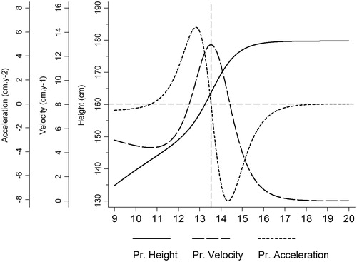
Table 1. Experimental parameters and rationale used in the simulation study.

Experiment	Description
1 Measurement error (σe = 0.5, 1, 2 cm)	The effect of measurement error under three different scenarios representing small (σe = 0.5 cm), medium (σe = 1 cm) and large measurement error (σe = 2 cm). The aim is to replicate the precision that may be achieved: under strict laboratory settings using specialist equipment, in field experiments using specialist equipment and field experiments using home based measuring equipment, respectively.
2 Sample size (J = 100, 500, 1000)	The effect of differing sample sizes, using small (J = 100), medium (J = 500) and large (J = 1000) samples sizes to reflect the variety of research studies from small scale project and trials, to larger cohort studies.
3 Measurement frequency (I = 40, 20, 10, 5)	The effect of the frequency of measurement occasions; which ranged from I = 40, 20, 10, 5, i.e. quarterly, biannual, annual and biennial measurement occasions.
4 Measurement balance (I = 10, 5)	The effect of moving from regular to irregular measurement occasions when I = 10 or I = 5 and measurements could occur in any quarter of the year. Measurement occasions were irregular between individuals, but regular within the individual, i.e. those measured in the first quarter of the year would always be measured in the first quarter of year, etc.

Methods used to estimate age at peak height velocity

Preece & Baines model 1 (PBGM)

The PBGM is a five parameter, non-linear model of height estimated for each individual in the cohort (Preece & Baines, 1978). Separate models are fitted for each individual in the dataset. Using the analytical solution for velocity and acceleration, age at PHV was estimated for each individual (Sayers et al., 2013).

Multi-level linear models using fractional polynomials (MLM-FP)

The MLM-FP is a simple extension of the multi-level linear model using conventional polynomials, similar to the model proposed by Goldstein (1986). The MLM-FP approach selects the best fitting polynomial terms of age from a given set and number (degrees) of terms (Royston & Altman, 1994). A detailed description of the model fitting and selection procedure is described in the Supplementary material. Following the selection of the best-fitting model, analytical solutions for velocity and acceleration are applied to calculate age at PHV and its confidence interval.

Superimposition by translation and rotation (SITAR) model

The SITAR model is a non-linear multi-level model with natural cubic splines, which estimates the population average growth curve and departures from it as random effects (Cole et al., 2010). The SITAR model uses three parameters which have direct interpretations: size, tempo and velocity of growth (Cole et al., 2010). PHV is identified using numerical differentiation of the individually predicted growth curves, with age at PHV being the age at which the maximum velocity is observed.

Principal analysis by conditional expectation (PACE)

PACE is an extension of functional principal components analysis which allows the inclusion of sparse and irregularly spaced longitudinal data (Yao et al., 2005). Derivative estimation using this method has previously been developed (Liu & Muller, 2009; Muller & Yao, 2010) such that individual velocity and acceleration trajectories can be predicted. Age at PHV is found by recording the age at which PHV is observed.

Summary statistics of interest

Bias was assessed at the level of the individual within each simulated dataset; mean bias, interquartile range of bias and 95% range of bias were calculated. Bias in age at PHV defined as Additionally, each method’s ability to preserve the ranking of age at PHV was assessed using Spearman’s rank correlation. To assess model fit, we compare bias in height at PHV defined as

Simulation implementation

All data were generated using Stata 12.1. (StataCorp, 2009) The MLM-FP were fitted in MLwIN 2.26 (Rasbash et al., 2009) via the runmlwin Stata command (Leckie & Charlton, 2011) and the individual predictions of velocity and acceleration for these models were calculated in Stata 12.1. SITAR models were fitted in R v2.7 (R Development Core Team, 2012) using the sitar package developed by Professor Tim Cole and PACE was fitted in MATLAB v7.14 (MATLAB, 2012). Annotated code and additional information is given in the Supplementary material.

The Preece & Baines growth model 1 was fitted to the data and age at PHV was estimated for each simulated dataset using a recently developed Stata command (Sayers et al., 2013). This Preece & Baines model is different to the DGP (P&B growth model 2).

Christ’s Hospital school data analysis

In total, 126 897 height measurements were available from 3123 boys who attended the school between 1939 and 1968. The cohort has been described in detail elsewhere (Sandhu et al., 2006). In this study we applied each of the four methods described above to these longitudinal data and then estimated age at PHV for each child. Pearson’s correlation was then used to assess the level of agreement between the methods. The time to fit the model was also recorded.

Comparing results between simulation and Christ’s Hospital school results

Bias could not be compared using the real data, since true age at PHV was not known in the Christ’s data. Thus, to compare results from our simulation study and real data example, we measured the level of agreement between methods in the simulated data. This was carried out in just those simulations which were most similar to the Christ’s data, i.e. 10 irregular repeated measures per individual.

Results

Results with respect to bias in age at PHV are presented in Figure 2. Each panel represents mean, inter-quartile range of bias and 95% range of bias in age at PHV on average across the simulated datasets. Results are described in comparison to the reference simulation, which has measurement error e_ij = 1 cm, sample size J = 1000 (balanced) and I = 10 measurement occasions.

Figure 2. Mean bias with interquartile range and 95% range of bias for the Preece & Baines, multi-level models-fractional polynomial (MLM-FP), superimposition by translation and rotation (SITAR) and principal components analysis through conditional expectation (PACE) methods used to estimate age at PHV across different experimental scenarios.

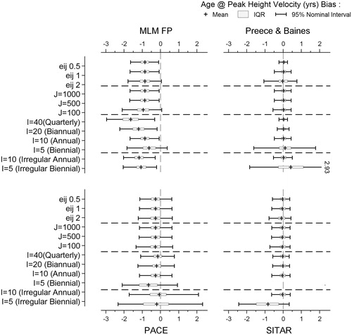
The PBGM modestly over-estimates the age at PHV by an average of 0.02 years, the interquartile range of bias is 0.25 years and the 95% range of bias is 0.92 years. Changes in measurement error (e_ij) have a small effect on the mean bias; however, the interquartile range of bias and 95% range of bias both increase as e_ij increases. Changes in sample size (J) have little influence on the bias, interquartile range of bias or 95% range of bias. Changes in the number of measurement occasions (I) have little effect on the mean bias and they result in only modest increases in the interquartile range of bias when I ≥ 10 and a more substantial increase when I = 5 (interquartile range of bias = 0.65 (–0.22, 0.43) years). The effect of changes in I on 95% range of bias is more gradual, although there is a large increase when I = 5 (95% range of bias = 3.39 years). Imbalance in the data has very little effect on the results when I = 10, although when I = 5 bias, interquartile range of bias and 95% range of bias increase dramatically in comparison to balanced data (interquartile range of bias = 1.39 years, 95% range of bias = 2.72 years).

The MLM-FP under-estimates the age at PHV by an average of 0.85 years, interquartile range of bias is 0.46 years, and the 95% range of bias is 1.6 years. Changes in measurement error (e_ij) have very little effect on the mean bias and only modestly increase the 95% range of bias when e_ij is 2 cm. Similarly, changes in sample size (J) also have very little effect on results with only a minor increase in the mean bias, interquartile and 95% range of bias. However, changes in the number of measurement occasions (I) result in dramatic changes in bias, the bias is greatest and most variable when the frequency of measurement is highest (I = 40). Imbalance in measurements when I = 10 results in similar characteristics to when I = 20, i.e. 10 heights recorded at irregular measurement occasions lead to similar results as 20 heights recorded at the same time for a cohort of individuals.

SITAR modestly under-estimates the age at PHV by an average of 0.04 years, the interquartile range of bias is 0.31 years and the 95% range of bias is 1 year. Changes in measurement error (e_ij) have very little effect on the mean bias or IQRB and there is only a modest increase in the 95%RB when e_ij is 2 cm. Similarly, changes in the sample size (J) and the number of measurement occasions (I) have very little effect on results. However, the model completely fails to fit when I = 5 and data are balanced. Imbalance when I = 10 has very little effect on mean bias, interquartile range of bias and 95% range of bias compared to the balanced data. When I = 5 and data are imbalanced the model converges, however the results are biased (–0.83 years) and are very variable (IQR = 1.24, 95% range = 2.77 years).

PACE moderately under-estimates the age at PHV by an average of 0.28 years, interquartile range of bias is 0.5 years, and 95% range of bias is 1.78 years. Changes in measurement error (e_ij) have very little effect on the mean bias and there is only a modest increase in the 95% range of bias when e_ij is 2 cm. Similarly, changes in sample size (J) have very little effect on results, with only a modest increase in the 95% range of bias when J = 100. As the number of measurement occasions (I) reduces from I = 40 to I = 10 there is a modest increase in the mean bias and when I = 5 the variability of the bias is greatly increased. Imbalance in measurement occasions, either when I = 5 or 10, results in a reduction in bias, but greatly increases the variability in both the interquartile range of bias (1.4 years) and 95% range of bias (2.31 years).

Model failures

The PACE approach was very robust and results were obtained under all conditions (Table 2). Convergence in the MLM-FP was part of the selection criteria for picking the best model. However, non-convergence in the inverse prediction step was common using the automated method we implemented in Stata. The PBGM did not converge on all occasions and the proportion of models that failed greatly increased when measurements were infrequent (I = 5) and when measurement error (e_ij) became large. Non-convergence rates for SITAR increased with measurement error e_ij =2 and when sample size was small (J = 100) or measurements became infrequent (I = 5). The SITAR model did not converge when I = 5 with balanced data.

Table 2. Non-convergence rates of the central difference, Preece & Baines, MLM-FP, SITAR and PACE methods used to estimate age at peak height velocity across different experimental scenarios.

	Failed (%)
Experiment	PB	MLM-FP	SITAR	PACE
1. Measurement error
0.5 cm	0.45	4.02	0.1	0
1 cm	1.06	4.15	3.8	0
2 cm	7.09	7.26	61.3	0
2. Sample size
n = 1000	1.06	4.15	3.8	0
n = 500	1.07	7.63	8.7	0
n = 100	1.66	96.02	17.1	0
3. Measurement frequency
I = 40	0.26	13.92	1	0
I = 20	0.31	8.16	0.3	0
I = 10	1.06	4.15	3.8	0
I = 5	26.76	20.60	100	0
4. Measurement balance
Irregular I = 10	2.62	11.43	0.4	0
Irregular I = 5	41.93	99.90	28.1	0

Correlation between estimated and true PHV

All the approaches investigated had a high level of correlation between true and estimated age at PHV (ρ_spearman > 0.9) (Table 3), with moderate measurement error (e_ij = 1), annual measurement (I = 10) and large sample size (J = 1000). The correlation between true and estimated age at PHV falls when measurement error is large (e_ij = 2), when measurement occasions are infrequent (I = 5) and more so when they are both infrequent (I = 5) and unbalanced. The MLM-FP approach is the only approach which occasionally results in an inverse correlation between the true and estimated age at PHV. The PBGM PACE approaches demonstrated low correlations between true and estimated age at PHV when data were infrequent (I = 5) and unbalanced, ρ_spearman < 0.4.

Table 3. Spearman’s rank correlation between the true age at PHV and the age at PHV estimated using the central difference, MLM FP, SITAR and PACE methods across different simulated scenarios.

	Spearman correlation (95% confidence interval)^1
Experiment	PB	MLM-FP	SITAR	PACE
1. Measurement error
0.5 cm	0.99 (0.99–1.00)	0.94 (0.93–0.95)	0.97 (0.97–0.98)	0.95 (0.94–0.96)
1 cm	0.98 (0.97–0.98)	0.94 (0.93–0.95)	0.97 (0.96–0.97)	0.95 (0.93–0.95)
2 cm	0.90 (0.88–0.92)	0.91 (0.90–0.92)	0.95 (0.94–0.96)	0.93 (0.91–0.94)
2. Sample size
n = 1000	0.98 (0.97–0.98)	0.94 (0.93–0.95)	0.97 (0.96–0.97)	0.95 (0.93–0.95)
n = 500	0.98 (0.96–0.98)	0.94 (0.92–0.95)	0.97 (0.96–0.97)	0.94 (0.93–0.96)
n = 100	0.97 (0.95–0.98)	0.93 (0.89–0.96)	0.96 (0.94–0.98)	0.94 (0.27–0.96)
3. Measurement frequency
I = 40	0.99 (0.99–0.99)	0.86 −(0.70–0.92)	0.97 (0.96–0.98)	0.96 (0.95–0.96)
I = 20	0.99 (0.98–0.99)	0.91 (0.82–0.93)	0.97 (0.96–0.97)	0.95 (0.27–0.96)
I = 10	0.98 (0.97–0.98)	0.94 (0.93–0.95)	0.97 (0.96–0.97)	0.95 (0.93–0.95)
I = 5	0.76 (0.72–0.80)	0.93 (0.00–0.94)	0.00 (0.00–0.00)	0.73 (0.66–0.81)
4. Measurement balance
Irregular I = 10	0.97 (0.96–0.97)	0.94 (0.92–0.95)	0.97 (0.96–0.97)	0.95 (0.10–0.96)
Irregular I = 5	0.39 (0.32–0.44)	0.91 (0.89–0.93)	0.86 (0.83–0.89)	0.26 (0.01–0.87)

PB: Preece & Baines model; MLM-FP: multi-level models with fractional polynomials; SITAR: superimposition by translation and rotation; PACE: principal components analysis through conditional expectation.

Bias in height at PHV

Table 4 displays bias in estimating the true height at peak height velocity and so allows us to see how well each model fits the height data. The Preece & Baines method achieves the lowest bias in height estimated at the peak height velocity, at just 0.17 cm on average (95% range of bias = –4.19, 3.66 cm). SITAR slightly under-estimates the height at PHV, with an average bias of –0.26 cm (95% range of bias = –4.51, 3.52 cm). PACE under-estimates height by 1.73 cm (95% range of bias = –7.01, 3.83 cm), while fractional polynomials have the highest bias with an over-estimate of 6.15 cm (95% range of bias = 1.34, 11.91 cm).

Table 4. Bias in height at PHV using the Preece & Baines, MLM FP, SITAR and PACE methods across different simulated scenarios.

	Bias in height (cm) at peak height velocity (95% range of bias)^1
Experiment	PB	MLM-FP	SITAR	PACE
1. Measurement error
0.5 cm	0.24 (−2.09–1.96)	6.15 (1.37–11.80)	−0.14 (−4.29–3.54)	−1.73 (−6.96–3.83)
1 cm	0.17 (−4.19–3.66)	6.15 (1.34–11.91)	−0.26 (−4.51–3.52)	−1.73 (−7.01–3.83)
2 cm	−0.28 (−8.91–5.98)	6.15 (1.09–12.10)	−0.74 (−5.28–3.27)	−1.76 (−7.21–3.85)
2. Sample size
n = 1000	0.17 (−4.19–3.66)	6.15 (1.34–11.91)	−0.26 (−4.51–3.52)	−1.73 (−7.01–3.83)
n = 500	0.17 (−4.24–3.64)	6.19 (1.30–11.99)	−0.24 (−4.58–3.55)	−1.74 (−7.08–3.83)
n = 100	0.17 (−5.00–3.66)	6.68 (0.36–12.53)	−0.24 (−5.18–3.56)	−1.79 (−7.75–3.72)
3. Measurement frequency
I = 40	0.22 (−2.07–2.03)	11.02 (2.15–20.61)	−0.08 (−4.05–3.27)	−1.14 (−6.12–4.13)
I = 20	0.22 (−2.87–2.74)	8.41 (1.32–17.02)	−0.03 (−4.10–3.41)	−1.62 (−6.99–3.97)
I = 10	0.17 (−4.19–3.66)	6.15 (1.34–11.91)	−0.26 (−4.51–3.52)	−1.73 (−7.01–3.83)
I = 5	−0.25 (−25.51–11.27)	4.73 (−0.02–10.73)		−3.72 (−11.41–3.98)
4. Measurement balance
Irregular I = 10	0.12 (−4.87–4.36)	8.23 (2.68–15.46)	−0.19 (−4.68–3.65)	−1.48 (−9.32–6.40)
Irregular I = 5	0.45 (−33.97–15.85)	7.44 (2.70–12.95)	−6.68 (−18.22–2.47)	−1.98 (−10.99–6.65)

PB: Preece & Baines model; MLM-FP: multi-level models with fractional polynomials; SITAR: superimposition by translation and rotation; PACE: principal components analysis through conditional expectation.

Christ’s Hospital school data

True age at PHV is not known for these data, but we present the results from each method in Table 5. Mean estimated age at PHV ranged from 13.21 years (PACE) to 14.26 years (SITAR). The strongest agreement was between the SITAR and MLM-FP methods, with ρ_pearson = 0.81 in the Christ’s Hospital data. The Preece & Baines method had the weakest association with the other methods, with ρ_pearson ranging from 0.07 (with PACE) to 0.20 (with SITAR). Runtime varied between methods; SITAR 20 minutes, MLM-FP took 1 hour to select the best model and less than 1 minute to fit it, PACE 6 hours and Preece & Baines 24 hours. Preece & Baines failed to converge for 336 children (11%), while all other methods reached convergence.

Table 5. Average age at PHV for the Christ’s Hospital school data, with Pearson’s correlation coefficients between estimated age at PHV from each pair of methods.

Method	Age at PHV	95% confidence interval	Runtime	PB	MLM-FP	SITAR	PACE
PB	12.70	12.62–12.78	24 hours	1	–	–	–
MLM-FP	13.44	13.40–13.48	1 hour	0.1782	1	–	–
SITAR	14.26	14.22–14.30	20 minutes	0.1974	0.8105	1	–
PACE	13.21	13.16–13.25	6 hours	0.0734	0.3298	0.3524	1

PHV: peak height velocity; PB: Preece & Baines model; MLM-FP: multi-level models with fractional polynomials; SITAR: superimposition by translation and rotation; PACE: principal components analysis through conditional expectation.

In the simulated data, the level of agreement was much higher than in the Christ’s data (Table 6). Each pair of methods, excluding PACE, had an average correlation of over 0.86. PACE seemed to least agree with the other methods, with average correlations between 0.6 and 0.7.

Table 6. Pearson correlation coefficients between estimated age at PHV in the simulation study.

Method
	P & B	MLM-FP	SITAR	PACE
PB	1	–	–	–
MLM-FP	0.87 (0.04)	1	–	–
SITAR	0.93 (0.03)	0.90 (0.04)	1	–
PACE	0.63 (0.34)	0.63 (0.38)	0.68 (0.34)	1

PB: Preece & Baines model; MLM-FP: multi-level models with fractional polynomials; SITAR: superimposition by translation and rotation; PACE: principal components analysis through conditional expectation.

Discussion

We have demonstrated the strengths and weaknesses of different methods used to estimate the age at peak height velocity (PHV) in childhood growth data. Age at PHV bias was smallest using the Preece & Baines and SITAR methods in nearly all experimental scenarios. Height at PHV bias was also smallest using these two approaches. Comparing these two, the SITAR method was much faster when fitting to the Christ’s Hospital data (20 minutes vs 24 hours) and the Preece & Baines method is similar to the model which generated our simulated data. The efficiency, flexibility and consistency of estimates using the SITAR approach make it an ideal method for exploring hypotheses which relate to the age at PHV. However, the SITAR approach had the highest rate of convergence problems. When measurement error was large (2 cm) only 40% of models successfully converged and when the number of measurement occasions were balanced and biennially spaced, model convergence was not possible. Therefore, the utility of this method using noisy or coarsely spaced balanced data may be limited. The PACE model was the most reliable (i.e. found an age at PHV for all simulations). The MLM-FP approach consistently had the greatest bias across experiments. Despite the increased complexity and flexibility from using fractional polynomials opposed to conventional polynomials, models were not sufficiently flexible to capture an individual’s underlying growth trajectory and accurately estimate their age at PHV. Furthermore, when assessing the correlation between true and estimated PHV, the MLM-FP was the only approach to result in inverse correlations, indicating that this approach should be used with caution.

Our results also illustrate a number of potential trade-offs when designing a study or choosing a method to estimate age at PHV. For example, the PBGM results demonstrate that study designs which have small measurement error and annual measurements can be used to estimate age at PHV with a similar degree of accuracy to study designs with higher frequency measurements (quarterly) and large measurement error. The MLM-FP method illustrates the consequences of using methods which respond to local changes in the data with global changes to the model, e.g. as measurement frequency increases the noise in estimated derivatives also increases.

Despite the limitations associated with each of the approaches investigated, the ability of nearly all approaches to preserve the ranking between true and estimated age at PHV is good, with Spearman correlations typically greater than 0.9. Therefore, the use of age at PHV estimated by any method in stratum-specific control of confounding should be effective (Greenland et al., 1999). Comparing the real and simulated results, we see an overall increase in the level of agreement when analysing simulated data. This is probably due to the ‘cleaner’ simulated data, with potentially more measurement error and irregular measurement in the Christ’s Hospital data. PACE has low levels of agreement with most other methods in both the real and simulated data, while SITAR and MLM-FP have relatively high levels of agreement in both the real and simulated scenarios.

There are several approaches which have been developed to mathematically model human height before (Count, 1943; Deming, 1957; Jenss & Bayley, 1937; Marubini et al., 1971) and after (Jolicoeur et al., 1988; Shohoji & Sasaki, 1987) the PBGM (Preece & Baines, 1978) which we have included for comparison here. The lack of comparison among these methods and with other non-parametric options (e.g. cubic splines) is a major limitation of our study. However, the availability of software to implement Preece & Baines (Sayers et al., 2013) influenced our decision on which of these structural models to include. The performance of the PBGM should highlight the benefits of implementing older approaches into modern software packages over using easily available but less flexible methods (i.e. fractional polynomials).

Our simulation study has extensively explored a variety of modelling approaches and experimental scenarios which may affect the design or implementation of studies investigating childhood growth. We have generated data from a biologically plausible model, which is consistent with the descriptions in the literature. However, the simulation study could be extended to explore other growth models, non-parametric models (e.g. restricted cubic splines) and the effect of different patterns of missing data. Also, we have not investigated the effect of using estimated age at PHV as a primary exposure in subsequent models or its use to control for confounding. Furthermore, the similarity between the data generating process and the PBGM (i.e. PBGM is a special case of the DGP when γ = 1) has likely resulted in over-optimistic model performance in comparison to other modelling approaches which are less closely related. This is evident when comparing the level of agreement between our simulated and real data results. The potential use of SITAR and PACE methods would be enhanced if the uncertainty of the estimates of age at PHV could be incorporated into their calculation.

Conclusion

Both SITAR and the PBGM are useful models for adolescent growth and provide unbiased estimates of age at PHV. The PBGM may provide an unbiased fit, but is computationally inefficient since each child needs to be modelled separately, so its use in large cohorts will take time. When designing a study to measure adolescent growth, the frequency of measurement occasions should be greater than five. Attempting to minimise measurement error will reduce bias and facilitate model convergence and increasing measurement frequency will also enhance model performance. Balancing the cost of reducing measurement error or increasing measurement frequency should be considered carefully.

Acknowledgements

AJS is funded by Medical Research council grant MR/L011824/1. AS was funded by MRC grant G1000726. Christs Hospital school data follow-up was funded by University of Bristol and the Medical Research Council. The authors would like to thank Professor Yoav Ben-Shlomo for use of the Christs Hospital school data.

Disclosure statement

No potential conflict of interest was reported by the authors.

Additional information

Funding

AJS is funded by Medical Research council grant MR/L011824/1. AS was funded by MRC grant G1000726. Christs Hospital school data follow-up was funded by University of Bristol and the Medical Research Council.

References

- Baxter-Jones AD, Faulkner RA, Forwood MR, Mirwald RL, Bailey DA. 2011. Bone mineral accrual from 8 to 30 years of age: an estimation of peak bone mass. J Bone Miner Res 26:1729–1739.
- Bayley N, Pinneau SR. 1952. Tables for predicting adult height from skeletal age: revised for use with the greulich-pyle hand standards. J Pediatr 40:423–441.
- Bergsten-Brucefors A. 1976. A note on the accuracy of recalled age at menarche. Ann Hum Biol 3:71–73.
- Billewicz WZ, Fellowes HM, Thomson AM. 1981. Pubertal changes in boys and girls in newcastle upon tyne. Ann Hum Biol 8:211–219.
- Bock RD, Wainer H, Petersen A, Thissen D, Murray J, Roche A. 1973. A parameterization for individual human growth curves. Hum Biol 45:63–80.
- Cole TJ, Donaldson MD, Ben-Shlomo Y. 2010. SITAR-a useful instrument for growth curve analysis. Int J Epidemiol 39:1558–1566.
- Count EW. 1943. growth patterns of the human physique: an approach to kinetic anthropometry: part I. Hum Biol 15:1–32.
- Damon A, Bajema CJ. 1974. Age at menarche: accuracy of recall after thirty-nine years. Hum Biol 46:381–384.
- Damon A, Damon ST, Reed RB, Valadian I. 1969. Age at menarche of mothers and daughters, with a note on accuracy of recall. Hum Biol 41:160–175.
- Darelid A, Ohlsson C, Nilsson M, Kindblom JM, Mellstrom D, Lorentzon M. 2012. Catch up in bone acquisition in young adult men with late normal puberty. J Bone Miner Res 27:2198–2207.
- Deming J. 1957. Application of the gompertz curve to the observed pattern of growth in length of 48 individual boys and girls during the adolescent cycle of growth. Hum Biol 29:83.
- Demirjian A, Goldstein H. 1976. New systems for dental maturity based on seven and four teeth. Ann Hum Biol 3:411–421.
- Didcock E, Davies HA, Didi M, Ogilvy Stuart AL, Wales JK, Shalet SM. 1995. Pubertal growth in young adult survivors of childhood leukemia. J Clin Oncol 13:2503–2507.
- Forwood MR, Bailey DA, Beck TJ, Mirwald RL, Baxter-Jones AD, Uusi-Rasi K. 2004. Sexual dimorphism of the femoral neck during the adolescent growth spurt: a structural analysis. Bone 35:973–981.
- Gastin PB, Bennett G, Cook J. 2013. Biological maturity influences running performance in junior Australian football. J Sci Med Sport 16:140–145.
- Goldstein H. 1986. Efficient statistical modelling of longitudinal data. Ann Hum Biol 13:129–141.
- Greenland S, Robins JM, Pearl J. 1999. Confounding and collapsibility in causal inference. Statis Sci 14:29–46.
- Greulich WW, Pyle SI. 1959. Radiographic atlas of skeletal development of the hand and wrist. Stanford: Stanford University Press.
- Hagg U, Taranger J. 1980. Menarche and voice change as indicators of the pubertal growth spurt. Acta Odontol Scand 38:179–186.
- Jenss RM, Bayley N. 1937. A mathematical method for studying the growth of a child. Hum Biol 9:556.
- Jolicoeur P, Pontier J, Pernin MO, Sempe M. 1988. A lifetime asymptotic growth curve for human height. Biometrics 44:995–1003.
- Kanefuji K, Shohoji T. 1990. On a growth model of human height. Growth Dev Aging 54:155–165.
- Khamis HJ, Roche AF. 1994. Predicting adult stature without using skeletal age: the khamis-roche method. Pediatrics 94:504–507.
- Krutchko RG. 1967. Classical and inverse regression methods of calibration. Technometrics 9:425.
- Leckie G, Charlton C. 2011. Runmlwin: stata module for fitting multilevel models in the Mlwin software package. Centre for Multilevel Modelling, University of Bristol.
- Liu BT, Muller HG. 2009. Estimating derivatives for samples of sparsely observed functions, with application to online auction dynamics. J Am Statist Assoc 104:704–717.
- Mao SH, Xu LL, Zhu ZZ, Qian BP, Qiao J, Yi L, Qiu Y. 2013. Association between genetic determinants of peak height velocity during puberty and predisposition to adolescent idiopathic scoliosis. Spine 38:1034–1039.
- Marubini E, Resele L, Barghini G. 1971. A comparative fitting of the gompertz and logistic functions to longitudinal height data during adolescence in girls. Hum Biol 43:237–252.
- Mason A, Malik S, Russell RK, Bishop J, Mcgrogan P, Ahmed SF. 2011. Impact of inflammatory bowel disease on pubertal growth. Horm Res Paediatr 76:293–299.
- MATLAB. 2012. Version 7.14 (R2012a). The Mathworks Inc., Natick, Massachusetts.
- Muller HG, Yao F. 2010. Empirical dynamics for longitudinal data. Ann Statis 38:3458–3486.
- Nielsen S. 1985. Evaluation of growth in anorexia nervosa from serial measurements. J Psychiatr Res 19:227–230.
- Preece MA, Baines MJ. 1978. A new family of mathematical models describing the human growth curve. Ann Hum Biol 5:1–24.
- Price DA, Shalet SM, Clayton PE. 1988. Management of idiopathic growth hormone deficient patients during puberty. Acta Paediatr Scand Suppl 347:44–51.
- R Development Core Team. 2012. R: A language and environment for statistical computing. R foundation for statistical computing, Vienna, Austria. Available online at: http://www.R-Project.Org/.
- Ramsay RO, Silverman BW. 2005. Functional data analysis. New York: Springer.
- Rasbash J, Charlton C, Browne WJ, Healey M, Cameron B. 2009. Mlwin version 2.24. Centre for multilevel modelling, University of Bristol.
- Reed RB, Berkey CS. 1989. Linear statistical model for gorwth in stature from birth to maturity. Am J Hum Biol 1:257–262.
- Roche AF. 1988. Assessing skeletal maturity of the hand-wrist: Fels method. Springfield: IL: Charles C Thomas.
- Roche AF, Wainer H, Thissen D. 1975. The Rwt method for the prediction of adult stature. Pediatrics 56:1027–1033.
- Royston P, Altman DG. 1994. Regression using fractional polynomials of continuous covariates: parsimonious parametric modeling. Appl Statis J R Statis Soc Ser C 43:429–467.
- Sandhu J, Ben-Shlomo Y, Cole TJ, Holly J, Smith GD. 2006. The impact of childhood body mass index on timing of puberty, adult stature and obesity: a follow-up study based on adolescent anthropometry recorded at Christ's hospital (1936–1964). Int J Obes 30:14–22.
- Sayers A, Baines M, Tilling K. 2013. A new family of mathematical models describing the human growth curve-erratum: direct calculation of peak height velocity, age at take-off and associated quantities. Ann Hum Biol 40:298–299.
- Sherar LB, Baxter-Jones AD, Faulkner RA, Russell KW. 2007. Do physical maturity and birth date predict talent in male youth ice hockey players? J Sports Sci 25:879–886.
- Sherar LB, Baxter-Jones ADG, Mirwald RL. 2004. Limitations to the use of secondary sex characteristics for gender comparisons. Ann Hum Biol 31:586–593.
- Shohoji T, Sasaki H. 1987. Individual growth of stature of japanese. Growth 51:432–450.
- StataCorp. 2009. Stata Statistical Software: Release 11, College Station, TX: Statacorp Lp.
- Tanner JM. 1962. Growth at adolescence. Oxford: Blackwell.
- Tanner JM, Whitehouse RH, Healy MJR. 1962. A new system for estimating skeletal maturity from hand and wrist, with standards derived from a study of 2600 health British children. Paris: International Children's Centre.
- Tanner JM, Whitehouse RH, Marshall WA, Healy MJR, Goldstein H. 1975. Assessment of skeletal maturity and prediction of adult height (Tw2 method). New York: Academic Press.
- Taranger J, Engstrom I, Lichtenstein H, Svennberg-Redegren I. 1976. Somatic pubertal development. Acta Paediatr 65(S258):121–135.
- Viner RM, Ross D, Hardy R, Kuh D, Power C, Johnson A, Wellings K, et al. 2015. Life course epidemiology: recognising the importance of adolescence. BMJ Publishing Group Ltd.
- Yao F, Muller HG, Wang JL. 2005. Functional data analysis for sparse longitudinal data. J Am Statis Assoc 100:577–590.