Evaluation and prediction of individual growth trajectories

Abstract

Background

Conventional growth charts offer limited guidance to track individual growth.

Aim

To explore new approaches to improve the evaluation and prediction of individual growth trajectories.

Subjects and methods

We generalise the conditional SDS gain to multiple historical measurements, using the Cole correlation model to find correlations at exact ages, the sweep operator to find regression weights and a specified longitudinal reference. We explain the various steps of the methodology and validate and demonstrate the method using empirical data from the SMOCC study with 1985 children measured during ten visits at ages 0–2 years.

Results

The method performs according to statistical theory. We apply the method to estimate the referral rates for a given screening policy. We visualise the child’s trajectory as an adaptive growth chart featuring two new graphical elements: amplitude (for evaluation) and flag (for prediction). The relevant calculations take about 1 millisecond per child.

Conclusion

Longitudinal references capture the dynamic nature of child growth. The adaptive growth chart for individual monitoring works with exact ages, corrects for regression to the mean, has a known distribution at any pair of ages and is fast. We recommend the method for evaluating and predicting individual child growth.

Keywords:

• Conditional SDS gain
• correlation model
• longitudinal growth reference
• multiple testing
• adaptive growth chart

Introduction

Evaluation and prediction of child growth are central activities in child health care. Conventional growth charts display the variation in growth in the population by age. Such charts offer limited guidance to address questions of parents and health professionals. Typical questions that parents have are: Is my child’s growth normal? Why is my child not following the centile line? What are the options to counter my child’s inhibited growth? Where will the next measurement be? Health professionals have questions like: Given what I know of the child, how will it develop in the future? Did the child grow normally since the last visit? What can I tell the parent about the child’s realised and future growth? While this article does not address all these questions directly, it offers tools that aim to advance the evaluation and prediction of individual growth curves.

Most published growth charts are distance references that portray the effects of age and sex on growth. Distance references have two primary uses. First, we can use them to evaluate the attained child’s growth at a particular age by comparing the child’s measurement to the population centiles in the chart. Second, we can apply distance references to remove the effects of age and sex on growth by transforming each measurement to a standard deviation score (SDS) or $Z$-score. As a result, effects on growth unrelated to age or sex will be easier to detect. Distance-based charts provide limited guidance on individual growth. Differences in tempo between children may produce distance references that are both biased and inefficient for studying growth during puberty (Tanner 1990, p. 187). At the individual level, it is better to look for unexpected changes in growth (e.g. failure-to-thrive, slow persistent deceleration, developmental delay) to identify potential pathology. This paper, therefore, concentrates on measures of change.

A simple measure of change is velocity, defined as $V=(Y_2-Y_1)/(T_2-T_1)$, where $Y_1$ and $Y_2$ are the attained size at ages $T_1$ and $T_2$. Low velocity appears on the distance chart as a downwards centile crossing. The level and variance of $V$ depend on age and sex, so proper interpretation of $V$ requires age- and sex-conditional references. Replacing $Y$ by $Z$ standardises the velocity scale to SDS per year, but its distribution depends on $T_1$ and $T_2$. Whereas a decelerating curve with a slope of −1 SDS/year indicates a dramatic height loss during childhood, the same value in infancy could fall within the normal range. Cole (1995) discussed a standardised version of velocity $Z^u=(Z_2-Z_1)/\sigma$, where $\sigma =\sqrt{2-2r}$ and $r$ is the correlation between $Z_1$ and $Z_2$. $Z^u$ has a standard normal distribution for all pairs of $\{T_1,T_2\}$ However, the problem with $Z^u$ is that it fails to account for regression to the mean. Generally, a child with a $Z_1$ value below zero has a higher expected growth rate than a child with a $Z_1$ value above zero. The strength of the effect depends on $r$.

Healy (1974) proposed a regression approach that conditions the reference on one or more known child factors. Prior measurements made at an earlier age are predictive in longitudinal settings. Early examples of references that condition previous data include Cameron (1980) and Berkey et al. (1983). Cole (1995) developed the conditional gain score $Z^g=(Z_2-r{Z}_1)/\sigma$ with $\sigma =\sqrt{1-r^2}$, which predicts $Z_2$ from a prior measurement $Z_1$. Conditioning may also involve multiple factors. For example, Thompson and Fatti (1997) proposed weight charts that adjusted the references to individual characteristics like height, age, and parity. The idea of conditioning can improve screening and monitoring tools with elevated sensitivity and specificity for detecting growth-related diseases.

Table 1 lists velocity and conditional indices for two measurements. The conditional SDS gain is the preferred measure in Table 1. It is the only measure that standardises for age and sex and that corrects for regression to the mean, a fundamental statistical phenomenon. Regression to the mean stems from the natural variation in weight gain from child to child. This variation is a combination of measurement error and actual biological differences in weight gain, so both components contribute to regression to the mean (Wright et al. 1994; Cole 1995). Moreover, especially for small values of $r$, its variance $1-r^2$ is low, so it is less sensitive to measurement error in $Z_1$ and $Z_2$ than alternatives. For these reasons, this paper concentrates on conditional SDS gain $Z^g$ as the measure of change.

Table 1. Overview of distance, velocity and conditional gain measures for longitudinal data.

Definition	Name	Advantages	Disadvantage
$Y_1$	Size at $T_1$	Simple	Age- and sex-dependent
$Z_1$	Size at $T_1$ in SDS	Standardised for age and sex	No information on growth
$V=(Y_2-Y_1)/(T_2-T_1)$	Velocity	Easy to calculate	Age- and sex-dependent
$W=(Z_2-Z_1)/(T_2-{}_1)$	Velocity in SDS	Standardised for time interval	Age- and sex-dependent
$Z^u=(Z_2-Z_1)/\sqrt{2-2r}$	Unconditional SDS gain	Standardised for age and sex	No regression to the mean
$Z^g=(Z_2-r{Z}_1)/\sqrt{1-r^2}$	Conditional SDS gain	Handles regression to the mean
		Standardised for age and sex

Despite its technological superiority, the conditional SDS gain has yet to be widely adopted. One reason for the slow update is that calculating by hand is difficult. In addition, there are no accepted standards or references for the time-to-time correlation matrix, i.e. the correlation matrix of the measurement taken at different ages. Another complication is that $Z^g$ is defined for two ages. In practice, we need to assess growth curves that consist of more than two measurements. In that case, there are multiple ways to select two ages. Calculating $Z^g$ for many age pairs leads to issues related to multiple testing. This paper, therefore, concentrates on extending $Z^g$ to work with more than two ages.

Wright et al. (1994) introduced the term thrive line. Until now, thrive lines have enjoyed limited popularity. For example, the overview by Scherdel et al. (2016) shows that many routine monitoring systems rely on decision rules with arbitrary cut points and unconditional SDS gain scores. Visual thrive line overlays exist that help interpret the growth chart, but these apply only to fixed age intervals. Technically, the thrive line is equivalent to a centile of the distribution of $Z^g$. This paper adopts the concept of the thrive line as a natural and elegant criterion for finding children experiencing failure to thrive.

This paper aims to develop, validate and demonstrate tools to evaluate and predict individual growth. The tools should work on growth curves with measurements taken at arbitrary ages, allow for a flexible choice of growth reference, take the dynamic nature of growth into account, be fast, intuitive, and easy to communicate, and have known statistical properties. Evaluation should inform us whether the observed growth is normal and assist in decision-making in cases where the child’s growth is unusual. Prediction should inform us about the likely growth path in the future and portray the inherent uncertainty associated with this prediction.

Section 2 (Materials) introduces the data used. Section 3 (Methodology) presents a definition of a longitudinal reference, extends $Z^g$ to include additional measurements, describes a fast algorithm to fit the relevant regression models, and explains how the method can work with arbitrary ages. Section 4 (Statistical Analysis) describes the quantitative techniques used to estimate the model parameters and validation statistics. Section 5 (Results) reports the results of the quantitative analysis. Section 6 (Applications) describes two applications: estimation of the overall referral rate and visualisation by the adaptive growth chart. Section 7 (Discussion) highlights the pros and cons and identifies areas for further research.

Subjects and methods

Materials

Data

The SMOCC study (Herngreen et al. 1994) collected weight measurements of a representative sample of 2151 Dutch children aged 0–2 between 1989 and 1990. Trained observers monitored and measured children at ten visits: birth and at months 1, 2, 3, 6, 9, 12, 15, 18, and 24. We selected the subset of 1895 children with a gestational age $>=$ 37 weeks and a minimum of four visits. Raw weights and heights were transformed into age- and sex-conditional $Z$-scores using references from the Fourth Dutch Growth Study (Fredriks et al. 2000).

Descriptive statistics

Table 2 contains the time-to-time correlations $\times$ 1000 calculated from the $Z$-scores in the SMOCC study subsample of term births. The number of measurements used to calculate Table 2 was 16,266 (height) and 17,618 (weight). We grouped the measurement ages into ten age bins and calculated the pairwise Pearson correlation matrix from the wide data.

Table 2. Time-to-time correlations times 1000 for Dutch children measured at birth, 1, 2, 3, 6, 9, 12, 15, 18 and 24 months. The upper triangle contains height correlations and the lower triangle represents weight correlations at different ages. Source data: Herngreen et al. (1994).

Month	0	1	2	3	6	9	12	15	18	24
0	–	702	663	580	524	462	440	425	390	374
1	790	–	856	791	691	614	598	585	563	518
2	655	902	–	844	745	671	646	630	587	560
3	532	776	909	–	803	741	715	687	651	627
6	412	587	696	817	–	862	829	784	747	702
9	384	508	589	683	884	–	890	843	814	759
12	390	486	544	615	793	926	–	895	863	818
15	395	480	526	579	727	867	938	–	884	843
18	397	467	503	556	681	808	880	933	–	866
24	392	462	499	535	636	751	828	881	918	–

Methodology

Longitudinal reference

A longitudinal reference $L$ describes the variation in growth between and within children. It is convenient to compose a longitudinal reference from two independent parts, a distance reference, and a time reference.

The distance reference $D$ describes how growth depends on sex and age (or on height, in the case of weight-for-height). Distance references derive from cross-sectional or longitudinal data or mixes of these. A significant application of $D$ is transforming measurements $Y$ into $Z$-scores, which removes the effects of age and sex. Assuming that $D$ is appro­priate for the sample of interest, then $Z$ follows a normal distribution with a zero mean and a unit variance at every age.

The time reference $R$ describes how $Z$-scores are related over time by the time-to-time correlation matrix $R$ of $Z$-scores. Time references can be calculated only from longitudinal studies. The idea of modelling distance and time references in successive stages is not novel. Pan and Goldstein (1997) emphasise that modelling on the scale of $Z$ is statistically convenient since it allows us to characterise the multivariate data structure fully.

We use the notation $L=\{D,R\}$ to refer to a longitudinal reference $L$. Note that we do not require that $D$ and $R$ stem from the same study. In this paper, we take $D$ as the height and weight references from the Fourth Dutch Growth Study (Fredriks et al. 2000) and define $R$ as the values in Table 2. The combination of $D$ and $R$ completely defines this study’s longitudinal reference $L$.

Conditional SDS gain for multiple time points

Let $Y_t$ stand for a measurement made at child age $t$ (in months). Once we have reference $L$ in place, the objective is to model $P(Y_t|Y_{t\prime <t},L)$, i.e. the distribution of outcome $Y$ at time points $t$ given any measurements observed at earlier time points $t\prime <t$. Subscript $t$ represents a vector of time points, possibly in the past, present or future. $P(Y_t|Y_{t\prime <t},L)$ describes the predictive distribution of $Y_t$ if $t$ lies in the future. For present and past $t$, the observed value $Y_t$ can be checked against the predicted distribution. We first consider this situation.

Two-time points

Suppose that we have height measurements $Y_2$ and $Y_6$ taken at ages of $t\prime =2$ (past) and $t=6$ (present) months, respectively. In a screening context, we wish to evaluate whether the realised height gain of the child during the interval $[2,6]$ is deficient. We check whether the probability of observing a value $Y_6$ given $Y_2$, $P(Y_6|Y_2,L)$, exceeds a pre-set cut point. Let the “hat notation” ${\stackrel{\wedge }{Y}}_6$indicate the predicted child height at month 6 given the child’s observed height at month 2 and reference $L$. We are interested in answering two questions: What is the expected score ${\widehat{Y}}_6$given a previous $Y_2$ and $L$? How far is realised $Y_6$ from the expected ${\widehat{Y}}_6$? The recipe for calculating the conditional SDS gain $Z_6^g$ is:

1. Transform measurements $\{Y_2,Y_6\}$ into $\{Z_2,Z_6\}$

2. Interpolate $r$ from $R$ at ages $t\prime =2$ and $t=6$

3. Calculate conditional SDS gain $Z_6^g$ as

$$Z_6^g=\frac{Z_6-r{Z}_2}{\sigma },\text{}\text{where}\sigma =\sqrt{\left(1-r^2\right)}$$

• Back transform ${\widehat{Z}}_6=r{Z}_2$ into ${\widehat{Y}}_6$

• Back transform $[{\widehat{Z}}_6\pm \left\{1,2\right\}\sigma ]$ into centiles -2, -1, +1 and +2 SD of the prediction interval for $Y_6$

• Assess the location of realised $Y_6$ within the prediction interval

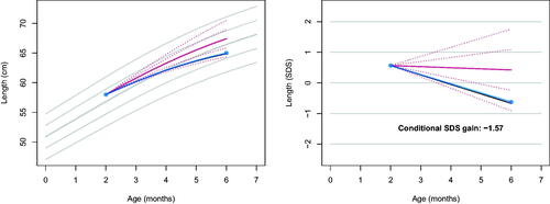
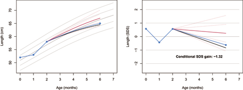
For example, suppose that $Y_2=58$, $Y_6=65$ and $r=0.745$, where $Y$’s unit is CM. Figure 1 plots the observed curve (solid, blue) and the predicted centiles at −2 SD, −1 SD, 0 SD, +1 SD, +2 SD of the prediction interval (in red) at $t\prime =2$. The left-hand plot depicts the observed and predicted curves in the measurement scale, whereas the right-hand side figure plots the same data in the SDS scale. The conditional SDS gain is $Z_6^g=-1.57$, just above the thrive line at the fifth centile (solid, black), at $Z=-1.645$.

Figure 1. Observed length curve (blue) plotted on top of the personalised reference (solid red: predicted growth; dotted red: centiles -2, -1, +1, +2 SD of the prediction interval), in the measurement scale (left) and the SDS scale (right). The conditional SDS gain at month 6 is equal to -1.57, just above thrive line at -1.64 (solid black). The grey lines in the background correspond to the height references for girls from the Fourth Dutch Growth Study.

Three time points

Growth faltering between months 2 and 6 is substantial in the example, but the value of −1.57 is slightly above the cut-off. Could our evaluation change if we use more than one historic measurement? To gain further insight, let us model $P(Y_6|Y_1,Y_2,L)$ and address the following questions: What is the expected score ${\widehat{Y}}_6$ given $Y_1$, $Y_2$ and $L$? How far is realised $Y_6$ from the expected ${\widehat{Y}}_6$? Suppose we have an additional measurement at month 1. The recipe for calculating the conditional SDS gain from time points $\{1,2,6\}$ is:

1. Transform measurements $\{Y_1,Y_2,Y_6\}$ into $\{Z_1,Z_2,Z_6\}$

2. Define time model $Z_6=Z_1{\beta }_1+Z_2{\beta }_2+ϵ$ with $ϵ\sim N(0,{\sigma }^2)$

3. Calculate regression weights ${\beta }_1=(r_{16}-r_{26}{r}_{12})/(1-r_{12}^2)$ and ${\beta }_2=(r_{26}-r_{16}{r}_{12})/(1-r_{12}^2)$

4. Calculate multiple correlation $r^2=(r_{16}^2+r_{26}^2-2r_{12}{r}_{16}{r}_{26})/(1-r_{12}^2)$

5. Calculate conditional SDS gain $Z_6^g$

$$Z_6^g=\frac{Z_6-(Z_1{\beta }_1+Z_2{\beta }_2)}{\sigma },\mathrm{where}\mathrm{ }\sigma =\sqrt{(1-r^2)}$$

• Then follow the previous recipe

Using $r_{16}=0.691$, $r_{26}=0.745$ and $r_{12}=0.856$ from Table 2, we obtain ${\beta }_1=0.198$, ${\beta }_2=0.575$ and $r^2=0.566$. Suppose $Y_1=56$ CM, then $Z_1=1.065$ so $Z_6^g=-1.76$.

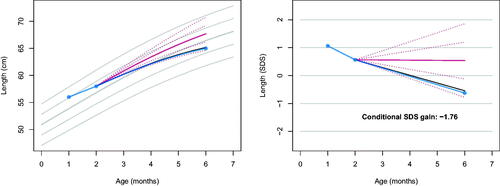
Figure 2 communicates that the curve shows a prolonged growth failure starting at month 1. The conditional SDS gain of −1.76 indicates a more severe growth deceleration than before. As a result of adding the additional measurement, the realised gain is below the fifth centile thrive line.

Figure 2. Observed length (blue) on the personalised reference (solid red: predicted growth; dotted red: centiles -2, -1, +1, +2 SD of the prediction interval) with three time points. The conditional SDS gain of -1.76 indicates a more severe drop-off (4 out of 100) than in Figure 1, thus providing an early warning of possible growth failure.

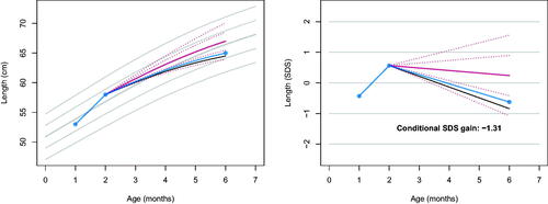
Figure 3 shows the same analysis, with one difference: $Y_1=53$ instead of $Y_1=56$. Now $Z_1=-0.432$, which changes $Z_6^g=-1.31$, so for these data 10 out of 100 have a lower $Y_6$ value. Compared to Figure 2, deceleration between months 2 and 6 now appears less alarming. The jagged nature of the trajectory in Figure 3 suggests that $Y_2$ may be too high, perhaps due to measurement error. The difference between Figures 2 and 3 illustrates that adding one extra observation affects the interpretation of the growth curve in an intuitive way.

Figure 3. Same as Figure 2, but now with an altered starting observation. Observed length (blue) on the personalised reference (solid red: predicted growth; dotted red: centiles -2, -1, +1, +2 SD of the prediction interval) with three time points. The conditional SDS gain of -1.31 indicates that drop-off is less severe than in Figure 1. The pattern suggests that the drop-off between months 2 and 6 may partly result from measurement error at month 2.

Estimation with more than three time points

The calculation of $\beta$ and ${\sigma }^2$ in recipe 2 becomes cumbersome for more than three-time points. The sweep operator (Beaton 1964; Goodnight 1979) is a fast and easy way to obtain these quantities for arbitrary time points. The operator calculates $\beta$ and ${\sigma }^2$ for any linear regression by applying simple pivots to the correlation matrix. Suppose we have the correlation matrix for time points 1, 2, and 6 months, and we wish to obtain ${\beta }_1$ and ${\beta }_2$ for predicting the outcome at month 6. The procedure below uses the sweep.operator() function from the R package fastmatrix (Osorio and Ogueda 2022). We start with the relevant $3\times 3$ correlation matrix:

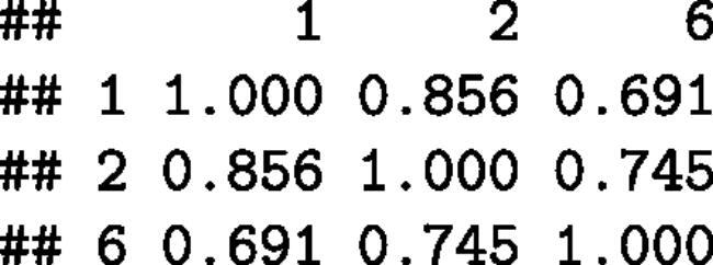
All variables are outcomes, but we may sweep out (“turn into in predictor variable”) columns 1 and 2 as follows:

We find the values of the $\beta$ and ${\sigma }^2$ parameters in the third column of the calculated result matrix s. The two regression weights ${\beta }_1$ and ${\beta }_2$ are $\{0.198,0.575\}$, and ${\sigma }^2$ equals $0.434$.

Application of the sweep operator to the time-to-time correlation table generalises the conditional SDS gain to any number of time points. For example, Figure 4 adds a birth length of $52$ cm to the curve. Note that the conditional SDS gain of −1.32 is similar to the previous model, which included two historical points. Adding birth length here had only a minimal impact on the evaluation.

Figure 4. Same as Figure 3, but now with an additional observation at birth. The conditional SDS gain of -1.32 is similar in size as in Figure 3, suggesting that including birth length does not add new information.

Arbitrary observation ages

Until now, the text presented examples where the measurement ages coincide with tabulated time points in $R$. In reality, the measurement ages and tabulated time points will differ. To make it useable, our model needs to work with arbitrary ages.

Correlation models express the correlation $\rho (t_1,t_2)$ between two Z-scores $Z_1$ and $Z_2$ at successive ages $t_1$ and $t_2$ as a function of those ages. The Cole correlation model (Cole 1995) describes the Fisher-transform $\varphi =\frac{1}{2}\text{log}\left((1+\rho )/(1-\rho )\right)$ of the correlation $\rho$ as a function of the sum $(t_1+t_2)$, the difference $(t_2-t_1)$, the reciproke $(t_2-t_1{)}^{-1}$ and includes two multiplicative terms. If $V_1=\log ((t_1+t_2)/2)$, $V_2=\log (t_2-t_1)$ and $V_3=1/(t_2-t_1)$ the model $$\varphi \left(t_1,t_2\right)={\beta }_0+{\beta }_1{V}_1+{\beta }_2{V}_2+{\beta }_3{V}_3+{\beta }_4{V}_1{V}_2+{\beta }_5{V}_1^2+ϵ,ϵ\sim \text{N}\left(0,{\sigma }^2\right)$$ has six unknown parameters that need to be estimated from $R$. Once the model is fitted and applied to new $t_1$ and $t_2$, the outcomes can be back-transformed into the correlation scale as $\rho =(\exp (2\varphi )-1)/(\exp (2\varphi )+1)$.

Statistical analysis

The aims of the statistical analyses were 1) to estimate the parameters of the correlation model and 2) to validate the statistical properties of the proposed methodology.

The first task was to estimate the parameters of the correlation model from the data in Table 2. The shortest interval in the table is one month, so the fitted model will need to extrapolate outside the data when $t_2-t_1$ is shorter than one month. To stabilise the estimates for such intervals, we arbitrarily specified the correlation of any 3-day difference to be equal to 0.95.

The second task was to obtain insight into the statistical properties of the method in practice. We calculated the mean and the standard deviation of the empirical distribution of the conditional SDS gain $P(Z_t|Z_{t\prime },L)$ for two models, called LAST and ALL. Model LAST conditions on the most recent measurement, while model ALL conditions on all historic measurements since birth. We estimated the proportion of explained variance and percentage of observations below the thrive line at each visit.

Results

Correlation model estimates

Table 3 contains the parameter estimates of the Cole model fitted to the Fisher-transformed weight and height correlations in Table 2. The fit for weight is near perfect with a percentage of explained variance of 99.7 per cent. Height correlations (97.1 per cent) are more challenging to model, especially for correlations below 0.5. After back-transformation into the correlation scale, the standard deviation of the observed minus predicted correlations was equal to 0.012 and 0.043, respectively, for weight and height.

Table 3. Linear regression of Fisher transformed correlations between Z-scores as predicted by mean age and time gap (in months), fitted on the data in Table 2.

	Estimate	Std. Error	t value	Pr(>|t|)
Child weight
${\mathit{\beta }}_0$	1.539	0.014	107.172	0.000
${\mathit{\beta }}_1$	0.329	0.008	39.384	0.000
${\mathit{\beta }}_2$	−0.951	0.013	−72.454	0.000
${\mathit{\beta }}_3$	−0.190	0.004	−50.485	0.000
${\mathit{\beta }}_4$	0.143	0.004	40.345	0.000
${\mathit{\beta }}_5$	0.001	0.003	0.188	0.852
Child height
${\mathit{\beta }}_0$	1.329	0.036	36.443	0.000
${\mathit{\beta }}_1$	0.250	0.021	11.799	0.000
${\mathit{\beta }}_2$	−0.672	0.033	−20.185	0.000
${\mathit{\beta }}_3$	−0.104	0.010	−10.927	0.000
${\mathit{\beta }}_4$	0.105	0.009	11.697	0.000
${\mathit{\beta }}_5$	−0.003	0.007	−0.428	0.670

Note: Adj $r^2$ (weight) = 0.997, Adj $r^2$ (height) = 0.971, n = 45.

Validation

Table 4 summarises the mean and standard deviations of the $Z$-scores for weight and height relative to the Dutch references for the SMOCC data. As expected, most aggregates are close to 0 (mean) and 1 (sd). The empirical distribution of the conditional SDS weight and height gains $Z^g$ is close to the standard normal distribution. The SMOCC children are slightly heavier and taller than the references between months 2 and 6. Note that the weight gain at month 2 has a positive bias (0.416 and 0.453), which indicates that children grow faster than expected between months 1 and 2. Weight gain is slower between months 3 and 6. The empirical standard deviation of $Z^g$ tends to be smaller than 1.0 around month 12. The proportion of explained variance for child weight from visit-to-visit is around 80 per cent. An exception is month 3 due to the relatively large time gap between month 3 and month 6. For height, predictive accuracy hovers around 73 per cent. Finally, the observed percentage of children below the P5 thrive line is 4.1 (weight) and 4.5 per cent (height), close to the nominal percentage of 5 per cent. Differences are generally slight between models LAST and ALL.

Table 4. Mean (MEAN) and standard deviations (SD) of Z-scores $Z$ and conditional SDS gains $Z^g$, the proportion of variance explained $r^2$ and the percentage of children below the P5 for models LAST (only last measurement) and ALL (all historic measurements), aggregated by visits (in months).

			MEAN($Z^g$)		SD($Z^g$)		$r^2$		p < P5
Month	MEAN(Z)	SD(Z)	LAST	ALL	LAST	ALL	LAST	ALL	LAST	ALL
Child weight
0	0.028	1.237
1	0.008	1.025	−0.043	−0.044	1.098	1.097	0.575	0.575	7.1	7.1
2	0.153	0.997	0.416	0.453	1.058	1.080	0.802	0.808	2.8	2.4
3	0.151	0.964	−0.010	−0.112	0.993	1.002	0.821	0.829	4.5	5.4
6	0.032	0.913	−0.172	−0.188	0.938	0.944	0.719	0.730	4.6	5.1
9	0.006	0.926	−0.023	0.013	0.941	0.942	0.808	0.812	2.9	2.5
12	0.009	0.929	−0.027	−0.022	0.882	0.874	0.870	0.875	3.3	3.0
15	0.025	0.940	0.054	0.050	0.927	0.929	0.889	0.891	3.8	3.7
18	0.047	0.961	0.117	0.109	1.002	1.005	0.875	0.877	3.9	4.1
24	0.093	0.974	0.119	0.110	1.020	1.047	0.842	0.841	3.2	3.4
Total	0.056	0.994	0.046	0.039	0.999	1.009	0.793	0.796	4.0	4.1
Child height
0	−0.149	1.127
1	0.005	1.018	0.252	0.252	1.167	1.167	0.466	0.466	5.5	5.5
2	0.063	1.004	0.174	0.176	1.113	1.120	0.728	0.723	5.0	4.9
3	0.153	0.962	0.159	0.165	1.083	1.055	0.727	0.740	4.6	4.5
6	0.102	0.933	−0.051	−0.046	0.928	0.939	0.694	0.688	3.2	3.3
9	0.060	0.953	−0.032	0.003	0.937	0.941	0.767	0.775	3.2	3.0
12	0.058	0.966	0.009	0.063	0.951	0.932	0.804	0.818	3.7	4.2
15	0.094	0.994	0.071	0.152	1.039	1.016	0.801	0.820	5.1	4.8
18	0.077	0.998	0.013	0.022	1.102	1.079	0.782	0.801	6.5	5.9
24	0.127	1.031	0.138	0.206	1.111	1.145	0.740	0.749	4.7	4.2
Total	0.062	1.001	0.068	0.112	1.046	1.051	0.731	0.726	4.5	4.5

Note: n = 17,618 (weight), n = 16,266 (height), 1,895 term-born Dutch children.

Applications

We demonstrate two applications of the method. The first application studies the effect of multiple testing on the overall referral rate. The second application uses the conditional SDS gain to create an adaptive growth chart that adds two new graphical elements.

Overall referral rate

Suppose we refer a child if its conditional gain SDS at some age is below a pre-specified centile. We wish to study the statistical properties of a growth monitoring scheme with $k$ visits. What is the probability that we refer a child in any of those $k$ visits? Under successive independent assessments, we can calculate the theoretical answer as 1 - pbinom(0, k − 1, 0.05). For example, if $k=5$, we obtain a probability of 0.185. How accurate is the theoretical answer in practice for different $k$?

We calculated the percentage of children with a conditional SDS gain below the 5 per cent thrive line in one or more of 10 visits and compared the result to the cumulative binomial distribution. Table 5 specifies three base referral probabilities $P\in \{0.05,0.025,0.01\}$ and compares the theoretical answer to the actual proportions in the SMOCC data. The theoretical proportion rapidly grows as the number of evaluations increases. For example, if we refer if the conditional SDS gain is below −1.645 ($P=0.05)$, then the binomial predicts that a sequence of ten evaluations will refer 37.0 per cent of all children at least once. Although the realised percentages are lower (28.2 and 30.5 per cent), these referrals are unreasonably large parts of the population. Using a stricter cut-off of −2.326 ($P=0.01$) reduces the rate to a more reasonable 8.6 per cent.

Table 5. Percentage of children with at least one referral based on the evaluation of the conditional SDS gain for a growth monitoring scheme with 10 visits in the first two years. For three base probabilities (0.05, 0.025, 0.01) the table gives the probability according to the binomial distribution, the realised proportion for weight, and the realised proportion for height.

	p = 0.05			p = 0.025			p = 0.01
Month	Binomial	Weight	Height	Binomial	Weight	Height	Binomial	Weight	Height
0	0.0			0.0			0.0
1	5.0	7.2	5.5	2.5	3.7	3.1	1.0	1.7	1.2
2	9.8	9.0	10.3	4.9	5.3	5.6	2.0	2.6	2.2
3	14.3	14.0	14.2	7.3	8.6	7.7	3.0	4.8	3.0
6	18.5	17.8	16.8	9.6	10.4	9.0	3.9	5.7	3.8
9	22.6	19.5	19.4	11.9	11.2	10.0	4.9	6.1	4.1
12	26.5	21.7	21.9	14.1	12.4	11.5	5.9	6.5	5.2
15	30.2	24.2	25.0	16.2	13.6	13.3	6.8	6.8	6.1
18	33.7	26.8	28.4	18.3	14.9	16.5	7.7	7.5	7.7
24	37.0	28.2	30.5	20.4	16.0	18.2	8.6	8.4	8.9

Note: n = 17,618 (weight), n = 16,266 (height), 1895 term-born Dutch children.

The binomial provides a reasonably accurate representation of the realised proportions, especially for small base probabilities. The distribution appears as a workable approximation for calibrating referral proportions in a growth monitoring scheme. Table 5 suggests that we may change the base referral probability, but there are also other alternatives. For example, we can tailor cut-off values to different actions (e.g. planning an additional visit), reduce the evaluation moments to a subset of time points, or - more generally - specify different referral proportions at different ages. The sequential testing literature on alpha spending functions (Demets and Lan 1994) treats the problem in detail.

Adaptive growth chart

A frequently asked question among parents is how tall their child will be. We know that tall parents have tall offspring, but for a given child, an accurate answer depends primarily on the realised growth of that child. Prediction of future growth can help to set expectations and motivate healthy behaviour. This section explores the techniques proposed in this paper to draw personalised growth charts.

The conditional SDS gains conditions on realised child growth and predicts current growth from previous growth. The same technique also applies to future growth. We can augment the correlation table of measurements at past ages with a set of future ages and calculate a personalised growth chart from the augmented table.

Figure 5 presents an adaptive growth chart that combines four graphic elements, each with a specific function:

Figure 5. Adaptive growth chart for the same child at nine successive visits (top-left to bottom-right). A computer-generated dispay would show one panel at a time, so the elements change dynamically at every new measurement. Each panel contains four graphic elements: the child’s growth curve (blue line), the population reference band (light green), amplitude showing the conditional SDS gain (darker bars, left of last measurement) and the flag, personalised reference band of future growth one-year ahead for the child.

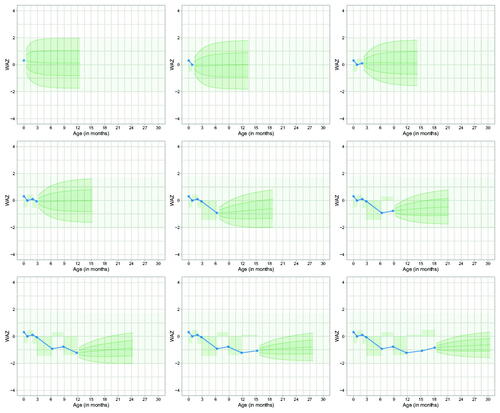
1. Blue points and lines: the child’s growth curve;

2. Reference band: area for evaluating the child’s data relative to a reference population;

3. Amplitude: area to evaluate how common the variation in the data over time is;

4. Flag: a mini-growth chart delimiting the area where we expect the child’s subsequent measurement one-year ahead.

We discuss each in turn.

The blue points represent the realised weight measurements adjusted for age (WAZ) for nine successive visits. Each visit adds one measurement. We see the top-left chart at birth, the top-middle chart at month 1, and the bottom-right chart at 18 months.

The reference band between the −2.0 SD and +2.0 SD delimits the normal range of the reference population. We expect that 95.4 per cent of the measurements of children of a given age will fall within this range. We can quickly evaluate whether some of the blue points are located outside the normal range and take appropriate action accordingly.

The amplitude element visualises a series of conditional SDS gains calculated for successive age intervals. The amplitude element is empty at birth and expands as a new measurement arrives. The element indicates how common the observed variability in the growth curve is. A zero amplitude means that the child grows precisely according to expectation. This could occur occasionally, but actual child growth typically deviates from the expectation. The level expresses the deviation’s direction and intensity during the age interval. A positive direction indicates that the child grew faster than expected, while the intensity level measures how much. The amplitude element provides a quick assessment of the commonness of variations in the data. We expect 95.4 per cent of the intensity levels to lie between the −2.0 SD and −2.0 SD centiles. Levels beyond this range could indicate that something is wrong, for example, that the child has rapidly lost weight due to an illness. However, an extreme value could also signal a measurement error in the data. If that is the case, we often see that the intensity level for a subsequent fidel measurement is extreme in the other direction. Measurement error will manifest itself by rapidly changing directions. Finding a run of four visits in the same direction is exceptional and could indicate slow growth failure, especially when combined with sizeable intensities. For this child, all levels fall nicely in the horizontal band, so the variation in the curve is normal.

The last element looks like a flag with the wind coming from the East. The flag element is a mini-growth chart that visualises the prediction interval for the next 12 months as centile lines −2 SD, −1 SD, 0 SD (median), +1 SD and +2 SD. More precisely, we expect with a confidence of 95 per cent that the subsequent measurement for the child will be located within the range of −2 SD to +2 SD. Centile lines grow apart with age because predicting further in time is more error-prone. The prediction interval is initially wide because infant growth at these ages is highly variable. As time goes by, predictions will become more accurate.

All elements work together. For example, consider the middle-left chart when the child is three months old. The 95 per cent prediction interval of the (yet unobserved) WAZ at month 6 varies roughly between −1.3 SD and +1.1 SD (read off the flag at month 6). Three months later, the realised value is slightly above −1.0 SD. This value locates approximately halfway between the −1.0 and −2.0 flag centile lines. The central chart for month 6 adds the −1.4 SD level to the amplitude element (read-off amplitude between months 3 and 6). We can quickly gauge whether the value falls outside the −2.0 SD to +2.0 SD range. Note that we use the same reference band for evaluating distance and gain, but one may set these levels independently when required. The prediction interval is updated with the new data point, and the cycle repeats.

The graph contains more information than might be needed for some purposes. Depending on the intended user, we could alter various aspects of the design. For example, a bouncing amplitude element could feel uncomfortable for parents. We could replace it with a smiley for periods when the conditional SDS gain falls within preset bounds or show a question mark or a frown when outside. Also, we could tweak the flag centiles as more straightforward interquartile ranges or even show only the predicted value without indicating uncertainty. To enhance compliance, we could tightly shrink the flag’s width to an age interval around the next scheduled visit. Another possibility to communicate the inherent predictive uncertainty is to plot the realised curves of children with a similar predicted value, a technique known as curve matching (van Buuren 2014; Toet et al. 2019). Another idea is to apply a one-sample runs test (Siegel and Castellan 1988) to separate measurement error from biological variation in a more formal way.

Discussion

The generalisation of the conditional SDS gain to the complete historical data requires us to specify three model components: a longitudinal reference, a correlation model to deal with arbitrary time points, and a prediction model for individual child data. The text below discusses these choices and their interdependencies.

The longitudinal reference consists of a distance and a time component. Both can be estimated from the same data but may derive from different samples. Although any distance reference defines a transformation from raw measurements into $Z$-scores, an improper reference choice can bias predictions. Suppose that the references are too low, then regression to the mean is more forceful for taller or heavier children, which results in a prediction that is too low and an SDS gain that is too high. As a rule of thumb, we suggest that the $Z$-score mean in the target sample should lie between −0.1 SD and +0.1 SD to prevent this bias.

The time component is a time-to-time correlation table. Table 2 was estimated by assigning each $Z$-score to the closest scheduled age. This procedure is sub-optimal because it assumes that the correlation is constant within bins, which may not hold. Binning may reduce correlations, but we do not yet know by what amount and what the impact would be in practice. The use of specialised estimation methods, as proposed by Xiao et al. (2018), Anderson et al. (2019), and van Buuren (2023) may improve upon simple binning. The Pearson correlation measures the strength between two normally distributed variables. Realise that applying a correlation for pairs of $Z$-scores that systematically deviate from bivariate normality may fail to capture subtle effects in growth.

The primary function of the correlation model is to produce a correlation table per child between ages of measurement. We used the parametrisation of the Cole correlation model and estimated the parameters from our data. Other correlation models with applications in child growth can be found in Lesaffre et al. (2000), Argyle et al. (2008) and Feng et al. (2020), and could potentially be used to improve the Cole model.

One striking result in Table 4 is that including more historical data points hardly raises the proportion of explained variance $r^2$. This finding is at variance with Ivanescu et al. (2017), who concluded, “Prediction performance increases substantially when using the entire growth history relative to using only the last and first observation” and “Subtle changes in the subject-specific history contain substantial additional information.” In contrast, in our approach, the inclusion of additional time points had negligible effects on $r^2$. Regression weights vanished after conditioning on the last two observations. Adding more than two measurements had little effect on the predicted value and the conditional SDS gain. It is an open question whether these results hold more generally. One reason why prediction may not get more precise could be that the correlation model smoothes out meaningful relationships beyond lag 2. It would be interesting to investigate this hypothesis in more detail. Finding a correlation model directly from the source data (instead of compressing the dynamic information into the correlation matrix) could shed light on the issue.

There is not yet much experience with formal growth prediction in preventive settings. My vision is that prediction intervals can help practitioners set expectations, motivate healthy behaviours, and communicate the variability in human growth. The predictive model produces a personalised mini-chart for the child’s subsequent measurement. The current model returns the area that contains a single future observation. Depending on the setting, one may also construct intervals in which all $m$ future observations will lie or contain $k$ out of $m$ (Hahn and Meeker 1991).

The predictive model is fast. For a given person, the algorithm calculates the personalised correlation matrix, the regression weights, the prediction and the SDS gain for each measurement. On an M1 Max processor, the calculations for all children in the data ($n=1895$) took 1.8 s, irrespective of the number of historical data points added. Thus, for a child with a growth curve of 10 measurements, we need about 1 millisecond to calculate the nine SDS gains.

A limitation of the current model is that it conditions only on previous outcomes. Including other time-varying outcomes or covariates (e.g. parental weights and heights, socio-economic factors) as predictors lead to sharper predictions. Technically, such extensions can be done in multiple ways. One straightforward possibility is to augment the time-to-time correlation matrix with the relevant factors.

The validation study revealed that the generalised conditional SDS gain has the expected statistical properties. Figures 2–4 show that the inclusion of the second last visit affects the value and interpretation of the conditional SDS gain. Cole (1995) said: “Strictly speaking, weight is better predicted if more than one previous weight is used.” Our study found only a slight increase in the proportion of explained variance. Still, using all historical information produces more informative gain scores less impacted by measurement error. In order to benefit, we suggest including at least the last two historical measurements in the conditional SDS gain.

The paper used the distance references $D$ from the Fourth Dutch Growth Study and calculated the time-to-time correlation matrices $R$ from the SMOCC data. Users from non-Dutch countries may want to use their national reference or adopt the WHO Child Growth Standards. For $D$, there are many options. However, only a few published estimates exist for $R$, so choices are minimal. We have yet to learn how $R$ differs across child populations. The SMOCC study involved a large longitudinal sample from 0–2 years from the general population. For the time being, we suggest using $R$ from Table 2 as a replacement.

Tracking individual child growth sounds easier than it is. This paper provides the theory, algorithms and tools for assembling an extensible modular monitoring system from simple principles. Setting a distance reference, a time-to-time correlation matrix, and a correlation model is enough to capture the dynamic nature of child growth. The adaptive growth chart for individual tracking works with exact ages, corrects for regression to the mean, and has a known distribution at any pair of ages. These properties turn the methodology presented here into an ideal vehicle for evaluating and predicting child growth.

The adaptive growth chart proposed in the Applications section incorporates two novel graphical elements: amplitude and flag. Incorporating these elements into one display will contribute to well-informed decision-making for parents, health professionals, and researchers.

Acknowledgements

The author wishes to thank the collaborators from the Child Health Clinics of the SMOCC cohort study for their contributions to the data collection.

Disclosure statement

No potential conflict of interest was reported by the author(s).

Data availability statement

The data used in this study are not public. The point of contact for the data is dr. Paul Verkerk (email: [email protected]).

Additional information

Funding

This study was financially supported by the Prevention, Work and Health research program, TNO, Leiden.

References

- Anderson C, Xiao L, Checkley W. 2019. Using data from multiple studies to develop a child growth correlation matrix. Stat Med. 38(19):3540–3554.
- Argyle J, Seheult A, Wooff D. 2008. Correlation models for monitoring child growth. Stat Med. 27(6):888–904.
- Beaton A. 1964. The use of special matrix operations in statistical calculus. Princeton, NJ: Educational Testing Service. Research Bulletin RB-64-51.
- Berkey C, Reed R, Valadian I. 1983. Longitudinal growth standards for preschool children. Ann Hum Biol. 10(1):57–67.
- Cameron N. 1980. Conditional standards for growth in height of British children from 5.0 to 15.99 years of age. Ann Hum Biol. 7(4):331–337.
- Cole T. 1995. Conditional reference charts to assess weight gain in British infants. Arch Dis Child. 73(1):8–16.
- Demets D, Lan K. 1994. Interim analysis: the alpha spending function approach. Stat Med. 13(13–14):1341–1352.
- Feng Y, Xiao L, Li C, Chen S, Ohuma E. 2020. Correlation models for monitoring fetal growth. Stat Methods Med Res. 29(10):2795–2813.
- Fredriks A, van Buuren S, Burgmeijer R, Meulmeester J, Beuker R, Brugman E, Roede M, Verloove-Vanhorick S, Wit J. 2000. Continuing positive secular growth change in The Netherlands 1955–1997. Pediatr Res. 47(3):316–323.
- Goodnight J. 1979. A tutorial on the sweep operator. Am Stat. 33(3):149–158.
- Hahn G, Meeker W. 1991. Statistical intervals: a guide for practitioners. New York: John Wiley & Sons.
- Healy M. 1974. Notes on the statistics of growth standards. Ann Hum Biol. 1(1):41–46.
- Herngreen W, van Buuren S, van Wieringen J, Reerink J, Verloove-Vanhorick S, Ruys J. 1994. Growth in length and weight from birth to 2 years of a representative sample of Netherlands children (born in 1988–89) related to socio-economic status and other background characteristics. Ann Hum Biol. 21(5):449–463.
- Ivanescu A, Crainiceanu C, Checkley W. 2017. Dynamic child growth prediction: a comparative methods approach. Stat Mod. 17(6):468–493.
- Lesaffre E, Todem D, Verbeke G, Kenward M. 2000. Flexible modelling of the covariance matrix in a linear random effects model. Biom J. 42(7):807–822.
- Osorio F, Ogueda A. 2022. fastmatrix: Fast computation of some matrices useful in statistics. R Package Version 0.4-124. https://CRAN.R-project.org/package=fastmatrix
- Pan H, Goldstein H. 1997. Multi-level models for longitudinal growth norms. Stat Med. 16(23):2665–2678.
- Scherdel P, Dunkel L, van Dommelen P, Goulet O, Salaün JF, Brauner R, Heude B, Chalumeau M. 2016. Growth monitoring as an early detection tool: a systematic review. Lancet Diabetes Endocrinol. 4(5):447–456.
- Siegel S, Castellan N.Jr 1988. Nonparametric statistics for the behavioral sciences. 2nd ed. New York, USA: McGraw-Hill Book Company.
- Tanner J. 1990. Foetus into man: physical growth from conception to maturity. 2nd ed. Cambridge, MA: Harvard University Press.
- Thompson M, Fatti L. 1997. Construction of multivariate centile charts for longitudinal measurements. Stat Med. 16(4):333–345.
- Toet A, van Erp J, Boertjes E, van Buuren S. 2019. Graphical uncertainty representa- tions for ensemble predictions. Inf Vis. 18(4):373–383.
- van Buuren S. 2014. Curve matching: a data-driven technique to improve individual prediction of childhood growth. Ann Nutr Metab. 65(3):227–233.
- van Buuren S. 2023. Broken stick model for irregular longitudinal data. J Stat Softw. 106(7):1–51.
- Wright C, Matthews J, Waterston A, Aynsley-Green A. 1994. What is a normal rate of weight gain in infancy. Acta Paediatr. 83(4):351–356.
- Xiao L, Li C, Checkley W, Crainiceanu C. 2018. Fast covariance estimation for sparse functional data. Stat Comput. 28(3):511–522.