Growing for good: producing a healthy, low greenhouse gas and water quality footprint diet in Aotearoa, New Zealand

ABSTRACT

Food production plays a central role in the health of humanity and our environment. New Zealand produces a large amount of food, but it is unknown if it can produce enough of the right crops in the places to better the health of New Zealanders, profitably, while maintaining New Zealand’s primary production exports and meeting ambitions to lower greenhouse gas (GHGs) emissions and nutrient losses to water. We tested two scenarios that aimed at delivering a healthy diet while maximising profit and minimising GHGs (climate-focused scenario) or losses of nitrogen (N) and phosphorus (P) to water (freshwater-focused scenario). Land use change was targeted to areas not currently meeting bottom lines for N or P loss but needed to spill over to other areas to meet dietary targets in both scenarios. The maximum cost of the required land use change was about 1% of the primary sector’s export revenues, and orders of magnitude less than the estimated savings for the health system from an optimised diet. We conclude that shifting productive land uses can help meet environmental targets for GHGs, N and P while saving money and improving the health of its people.

KEYWORDS:

• Eutrophication
• gross margin
• land use
• nitrogen
• phosphorus

Introduction

Food is at the centre of our health and the health of our environment. A shift towards processed foods and away from plant-based diets has coincided with a rise in cardiovascular disease, cancer, and diabetes which collectively now account for 73% of deaths worldwide (Roth et al. 2018). Replacing plant-based diets has increased livestock production and products (Swain et al. 2018). Livestock have been implicated in an increase in greenhouse gasses (GHG), mainly methane, and as a cause of poor water quality by increasing the loss of contaminants such as nitrogen (N) and phosphorus (P) from land to water (Steinfield et al. 2006).

Like many industrialised nations, New Zealand has reported a steady increase in the last 30 years in GHG emissions and an increase in N and P contamination of streams, rivers, and lakes. As of 2018, gross GHG emissions were 78.9 million tonnes of CO₂ equivalents (CO₂-e), representing a 24% increase on 1990. Emissions are roughly split between transport, manufacturing, and electricity generation (45%) and agricultural production (44% from methane and 9% from nitrous oxide). Emissions from agriculture, largely related to livestock farming, have increased by 8% (methane) and 54% (nitrous oxide) since 1990 (Statistics New Zealand 2021). Long-term monitoring of 77 sites draining almost half of New Zealand’s land area shows significant increases in dissolved nitrate-nitrite-nitrogen in 27 catchments from 1989–2014, while a snapshot of streams and rivers nationally in 2020 reported 95% of catchments in pastoral land cover exceeded guideline values for N, P and turbidity (derived from sediment) (Ministry for the Environment and Statistics New Zealand 2020b). This deterioration has corresponded with a change in livestock numbers and an increase in the intensity of land use management. For example, dairy cattle have increased from 3.8 million in 1994–6.5 million in 2017, and nitrogen fertiliser has increased from 59,000 tonnes in 1990–429,000 tonnes in 2015 (Fertiliser Association of New Zealand 2018; Livestock Improvement Corporation Limited and DairyNZ 2019; Ministry for the Environment and Statistics New Zealand 2020b).

In response to these changes, the New Zealand Government has enacted policies to reduce GHG emissions and improve the state of waterways. The amended Climate Change Response Act (New Zealand Government 2019) has set targets to reduce methane emissions by at least 10% by 2030 and 24-47% by 2050 compared to 2017 emissions and to reduce emissions of other GHGs to net zero by 2050. Policy for freshwater also set targets in the form of national bottom lines for maximum allowable concentrations of N and P either directly or indirectly (e.g. via concentrations of periphyton), and environmental standards for the maximum allowable application rates of nitrogen fertiliser to contiguous parcels of pastoral land (190 kg N ha⁻¹ yr⁻¹) (Ministry for the Environment 2020a). These limits come into effect in 2024.

Recognising that the effects of land use and management on water and air cannot be separated, the New Zealand Climate Commission estimated that some reductions in biogenic methane emissions would occur due to the implementation of freshwater policy. However, they also estimated that to meet targets, these changes would not be enough – requiring livestock numbers to reduce further by 13% and assuming that some land use would change to forestry (Climate Change Commission 2021).

New Zealand’s policy to reduce GHG emissions or improve water quality will act as a catalyst for land use change (Wang et al. 2021). In addition to converting land used for livestock to forestry, we could embrace international dietary trends to produce arable and horticultural crops with lower GHG and water quality footprints (Poore and Nemecek 2018). Although livestock production systems in New Zealand tend to be more efficient, losing less GHG per unit area or product than intensive international examples (Mazzetto et al. 2021), losses still tend to be greater than seen in the arable or some horticultural sectors (McDowell and Wilcock 2008; Norris et al. 2019) due to the significant contribution of enteric methane produced by ruminants (e.g. cattle, sheep, deer).

Recent work has examined what healthy and low GHG producing diets may look like in New Zealand (Drew et al. 2020). However, within a land use, the range of GHG and water quality footprint can range greatly depending on how well management matches land characteristics like soil type, slope, and climate. Land Use Suitability (LUS) is a concept that identifies the productive potential of land for a particular crop and assesses its contribution to causing water quality problems (McDowell et al. 2018). Using LUS can help plan for a transition to an alternative and profitable land use that has a much lower environmental impact.

International markets have long dictated what is grown in New Zealand, with some sectors exporting up to 95% of produce. New Zealand produce has long attracted a premium in many international markets owing to its high quality, safety and taste properties (Saunders et al. 2016). Together with an innovative workforce, strong returns have created well established value chains that may be resistant to change. With a small population of 5 million (in 2020), relative to land area, it is estimated that New Zealand produces food for 40 million people (KPMG 2017). However, because of imbalances in what is grown and needed, 40% of adults and 20% of children live in a household with severe to moderate food insecurity (Rush and Obolonkin 2020), leading to poor health outcomes . To improve health and environmental outcomes, the quantity and array of crops grown will be different from that produced now. The aim of this paper was to determine if New Zealand can produce a healthy diet while maintaining our primary export sector and moving towards meeting objectives for water quality and greenhouse gas emissions. We set and tested those objectives in two scenarios: one focused on using land use change to reduce GHG emissions (climate-focused), while the other used land use change to reduce water quality impact from N and P losses (freshwater-focused).

Materials and methods

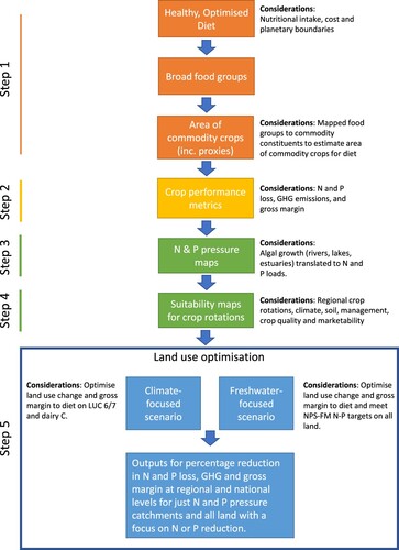
We tested the ability to grow a healthy diet within two scenarios where we optimised land use change according to gross margin to meet climate- and freshwater-focused objectives. This was done in five steps as outlined below and in Figure 1.

Figure 1. Schematic outline of the process followed to create and test the two scenarios to achieve a healthy diet.

Step 1: Healthy diet

Optimisation methods, as outlined in 2022b, were used to develop a healthy diet for the New Zealand population using the current New Zealand diet, as of the last Adult Nutrition Survey (2008/09), as a starting point (University of Otago and Ministry of Health 2011). Optimisation used equations that ensure that:

• average population diets met New Zealand food based dietary guidelines (Ministry of Health 2020) and nutrient guidelines for the minimum intakes of 17 micronutrients and three macronutrients and maximum intake for total fat, saturated fat, sugar and sodium (https://www.health.govt.nz/publication/nutrient-reference-values-australia-and-new-zealand);

• energy intake was within 10% of baseline energy intake.

• the cost to the consumer was below the baseline 2011 costs of the average diet; and diet-related GHG emissions were minimised and did not exceed the New Zealand-specific planetary boundary of 1.9486 kg CO_2-e person⁻¹ d−¹ for the baseline year of 2010 (Andersen et al. 2020).

• grams per food group were not more than twice the baseline intake to ensure a realistic intake.

Methods for how the GHG emissions per Adult Nutrition Survey food group were calculated have been published previously (Drew et al. 2020).

Optimisation was carried out in Microsoft Excel using an Excel add-in, ‘Solver’. The solver function worked with a group of cells, called decision variables (e.g. grams of fruit). Solver adjusted the values in the decision variable cells to satisfy the limits on constraint cells and produce the desired result for the objective cells (e.g. total sodium content of the diet). Optimisation was carried out by gender and ethnicity (Māori/non-Māori) and created an average diet for these four population subgroups. It should be noted that the optimised diet is an average diet for one day’s consumption by the whole adult population and the 185 food groups it draws on are from the last Adult Nutrition Survey (2008/09) (University of Otago and Ministry of Health 2011). Although some may find the list of foods acceptable or unacceptable, acceptability of diets and day-to-day eating habits were not taken into consideration.

Based on this diet, a list of food groups and amounts consumed was extrapolated to annual consumption at a national level (Cleghorn et al. 2022a). The grams of food groups produced by the optimisation were per person per day. They were totalled based on a national population of 5,116,300 people and 365.25 days per year.

The next step was to link foods to agricultural products. The modelling produced an optimised diet by broad food groups (31 in total in the baseline Adult Nutrition Survey (University of Otago and Ministry of Health 2011), 13 included in the optimised diet). The agricultural model and data about economic farm performance and environmental impacts related to types of farming and crops. To link performance and impact, each broad food group was assigned to one or more crops. We chose crops that represented the food groups directly (e.g. potatoes) or by the nearest available proxy for product or crop (e.g. breakfast cereals were considered 50 per cent wheat and 50 per cent oats, while onions were chosen to represent all alliums). The mapping of foods to crops is shown below in Supplementary Table S1.

For each broad food group, the amount required was multiplied by the percentage of the requirement being supplied by agricultural product (e.g. crop or livestock produce). The result was then adjusted to account for losses in postharvest handling and storage, processing and packaging, and distribution (Gustavsson et al. 2011), and then summed for each crop (Supplementary Table S2). We did not adjust the area required for an optimised healthy diet for some crops like wheat or barley where a variable proportion of production is used for animal feed instead of human consumption because of issues like inconsistent supply or low selenium concentrations in wheat (Curtin et al. 2008). Instead, we assume that existing supply (either domestic or bought in) is maintained and that inconsistent supply or low selenium concentration can be overcome resulting in >95% of new production being used for human consumption. The calculation produced an estimated annual farm-gate production of each crop required to meet the optimised diet.

The required crop production was converted to areas of each crop based on data on per-hectare production (Ministry for Primary Industries 2017; Plant and Food Research 2019; Reynish 2020; Monaghan et al. 2021). Production and the area required to meet the diet are given in Supplementary Table S1 and Table 1. For the most accurate data on current tonnage, yield and quality of different arable crops, readers are directed to data produced by the Arable Food Industry Council 2022

Table 1. Annual production, per hectare production required, and the crop areas required (and in addition to areas above current production) to grow the optimised healthy diet. Information is also given about the areas available for crop rotations, on average, within N and P pressure catchments. Refer to Table S3 for information on the crop rotations in major crop growing regions.

Land uses and crops	Production (t)	Current per ha production (t)	Area (ha) required for healthy diet (ha)	Area required above current production (ha)^a	Area provided by likely crop rotations within pressure catchments (ha)^b	Area provided by likely crop rotations outside of pressure catchments (ha)^b
Apples	358,477	61.0	5,877	−4,123	Na	Na
Broad beans	112,774	9.8	11,508	10,508	213,164	317,956
Carrots	91,682	85.0	1,079	−921	Na	Na
Dairy	84,253	1.2	72,867	−1,687,133	Na	Na
Oats	95,105	6.4	14,860	7,860	35,519	76,143
Onions	186,303	60.0	6,210	1,210	12,251	29,451
Citrus	325,204	35.0	9,292	7,292	−	7,292
Peas	207,543	9.0	23,060	9,060	213,164	317,956
Potatoes	689,652	65.0	10,610	610	3,423	8,755
Sheep/beef	8,036	0.3	26,785	−8,738,215	Na	Na
Wheat/barley	500,502	11.5	43,522	2,522	35,519	76,143

^a Negative values indicate that more area is already in production than required to meet the healthy diet.

^b These data are only for the targeted crop within a rotation. To calculate the total area occupied by the rotation, including non-target crops across New Zealand, divide the target crop area by 0.33, 0.37, 0.43, 0.43, 0.30, and 0.355 for Broad beans, Oats, Onions, Peas, Potatoes, and Wheat/Barley, respectively.

Step 2: Crop performance

To produce a healthy, low-GHG diet that fits within the New Zealand Government’s ambitions for GHG emissions and water quality, we collated the likely losses of N and P to water, and GHG emissions to air of proxy crops from a range of measured and modelled data. We also included forestry in this mix of crops, not as part of the low-GHG diet but to be used as a tool should other land uses not enable GHG or water quality targets to be met. We included data on their profitability as measured by gross margin (i.e. excluding costs associated with land rental or owner salaries, which are generally not reported). All data for the proxy crops (+ forestry) were sourced from the literature and are outlined in Table 2.

Table 2. Current area and the environment, production, and economic performance of agricultural product classes for a low GHG diet for New Zealand.

Crop class^a	Current area (km^2)	N loss (kg ha^−1 yr^−1)	P loss^b (kg ha^−1 yr^−1)	GHG loss (kg CO2-e ha^−1 yr^−1)	Production^c	Gross margin^d ($ ha^−1 yr^−1)	References
1-Dairy A	2,562	35	1.2	13330	1160	3,759	(Van der Weerden et al. 2018; Monaghan et al. 2021)
2-Dairy B	1,667	29	1.4	12881	1100	3,759	(Van der Weerden et al. 2018; Monaghan et al. 2021)
3-Dairy C	1,618	103	0.7	14506	1317	5,262	(Van der Weerden et al. 2018; Monaghan et al. 2021)
4-Dairy D	2,422	38	0.7	12492	1048	3,954	(Van der Weerden et al. 2018; Monaghan et al. 2021)
5-Sheep/beef A	10,334	8	0.5	448	1.4	199	(Hutchinson et al. 2019; Monaghan et al. 2021)
6-Sheep/beef B	7,920	17	1.1	3604	9.8	1392	(Hutchinson et al. 2019; Monaghan et al. 2021)
7-Sheep/beef C	8,714	5	0.3	2176	6.8	966	(Hutchinson et al. 2019; Monaghan et al. 2021)
8-Sheep/beef D	8,149	16	0.7	3714	10.1	1434	(Hutchinson et al. 2019; Monaghan et al. 2021)
9-Wheat	41	50	0.66	1643	11.5	2578	(Ryden et al. 1973; Barber et al. 2011; Norris et al. 2019)
10-Barley	56	28	0.12	1309	9.0	2064	(Evans 2002; Saunders et al. 2006; Norris et al. 2019)
11-Oats	7	74	0.33	1179	6.4	2286	(Ryden et al. 1973; Evans 2002; Rajaniemi et al. 2011; Norris et al. 2019)
12-Apple	10	18	0.48	673	61	18772	(Fenemor et al. 2015; Norris et al. 2019; Plant and Food Research 2019; Thomas et al. 2020)
13-Potato	10	88	0.16	1696	65	13050	(Norris et al. 2019; Plant and Food Research 2019; Thomas et al. 2020)
14-Onion	5	81	0.33	619	30	3053	(Norris et al. 2019; Plant and Food Research 2019; Thomas et al. 2020)
15-Peas	14	28	0.50	350	9	1080	(Norris et al. 2019; Plant and Food Research 2019; Thomas et al. 2020)
16-Carrot	2	30	0.13	431	85	3400	(Norris et al. 2019; Plant and Food Research 2019; Thomas et al. 2020)
17-Citrus	2	40	0.48	215	35	12872	(Tsushima et al. 2009; Plant and Food Research 2019; Thomas et al. 2020)
18-Bean	1	28	0.50	302	9.8	2830	(Evans 2002; Norris et al. 2019; Plant and Food Research 2019)
19-Plantation forestry	21,000	4	0.1	−25000	580	1150	(Cooper and Thomsen 1988; Davis 2014; Thomas et al. 2020)

^a Classes are designed to represent generic performance. Dairy A-D are sourced from Monaghan et al. (2021) for a Warm/Flat/Well drained/Moist typology in Waikato (A), Warm/Flat/Poorly-drained/Moist typology in Waikato (B), a Cool/Flat/Light soil/Irrigated typology in Canterbury (C), and a Cool/Flat/Well-drained/Moist typology in Southland. Sheep/beef A-D are sourced from Monaghan et al. (2021) for hill country typology in Marlborough-Canterbury (A), a hill country typology in Northland-Waikato-Bay of Plenty (B), a high country typology in Otago-Southland (C), and a finishing and breeding typology in Marlborough-Canterbury (D). Note that these typologies were compared and found to be similar to measured losses of N and P for the farm class (see Supplementary data in Monaghan et al. 2021).

^b Phosphorus losses for barley, potato, onions, peas, carrots, and beans are for subsurface flow only. Owing to a lack of data, P losses for apples are assumed to be the same as citrus.

^c Production is listed as stock units ha⁻¹ for dairy and sheep and beef classes and as t ha⁻¹ yr⁻¹ for all other crops. Production and gross margin for forestry were sourced from Farm Forestry New Zealand (nzffa.org.nz). Production data for arable crops are sourced from https://www.far.org.nz/assets/files/blog/files/c2bbd3c1-b18a-55dd-ba61-6126c8d5a939.pdf and from colleagues at the Foundation for Arable Research and Horticulture NZ.

^d Gross margins were sourced from Reynish (2020) for dairy, sheep and beef, wheat, barley, potatoes, and onions; the margin for apples were sourced from the Pipfruit Monitoring Programme (Ministry for Primary Industries 2017); the margin for oats came from the Foundation for Arable Research, while Horticulture New Zealand supplied margins for peas, carrot, citrus and beans. For sheep/beef classes A, B and D assume $142 per stock unit for Crossbred Ewe flock breeding own replacements, 155% lambing rate and $118 revenue per head, and $65.5 per head of beef cattle; sheep/beef class C assumes $142 per stock unit Merino Ewe flock breeding own replacements, $112 for meat and a 20-micron fleece for wool at $18.50 per head sold; Potato data are for the Agria variety.

To calculate GHG emissions for different crop types (and pastoral systems), we included biological emissions (methane and nitrous oxide) from livestock (enteric methane, excretal returns to soil), synthetic N fertiliser applied to land, and crop residues returned to land. For nitrous oxide emissions, both direct and indirect (via ammonia volatilisation and N leaching) emissions were included. For dairy systems we applied the relationship between amount of feed consumed/hectare (ha) and GHG emissions ha⁻¹ (Van der Weerden et al. 2018) while GHG emissions were estimated for sheep and beef systems based on revised stock units ha⁻¹ (Hutchinson et al. 2019). For arable and horticultural crops we applied the national inventory methodology (Ministry for the Environment 2021) and assumed all N fertiliser was non-urea based. We adjusted total GHG emissions associated with the loss of soil C with land use change to forestry from low producing pasture (sheep and beef), or from sheep and beef or high producing pasture (dairy) to arable or horticultural crops or forestry. We used coefficients for changes in soil C stocks for post-1989 planted forests (−14.1 t C ha⁻¹) and annual cropland (−16.2 t C ha⁻¹) (for arable and horticultural crops) relative to low producing grassland or high producing grassland (after adjusting for soil C losses compared to low producing grassland; −0.6 t c ha⁻¹) (McNeill et al. 2014; Ministry for the Environment 2021). We adjusted changes in soil C stocks, given for a 20-year period, to annualised losses as CO_2-eq. and consider our system was in equilibrium meaning that there was no change in soil C stocks within a given land use type.

Step 3: Pressure maps and scale

Pressure maps outline the magnitude of N and P loads exceeding a maximum allowable load for attributes within the NPS-FM (Supplementary Figure S1). The NPS-FM stipulates that limits and action plans are to be set within freshwater management units or parts thereof. Although the isolation of freshwater management units (FMUs) is well advanced, sub-FMU catchments that will be subject to limits and action plans are not. We therefore chose to delineate streams and catchments within FMUs at the fourth (Strahler) order.

Pressure maps identify critical points that cause all upstream areas to exhibit the same pressure. To manage the spatial area subject to land use optimisation for good water quality and low GHG emissions, we again focused on fourth order catchments which are under pressure at their outlet. In making this choice, we recognise that we may miss opportunities to optimise land use in some smaller streams that are under pressure within fourth order catchments that are not. For total N and P this represented the difference between the current load and the load corresponding to the C band for periphyton in streams and rivers and phytoplankton in lakes and estuaries.

The presence and magnitude of pressure differs by contaminant, meaning that a catchment may be under pressure by one or both contaminants. For simplicity, we chose to optimise land uses for N and P in separate scenarios but also recorded for each scenario the effect of changing land use on reducing the load of P and N (see later), respectively. Our calculations did not include any change to or contribution from urban land use nor for mitigations over and above those already accounted for within existing land use classes. For example, classes Dairy A through D were assumed to have already implemented stock exclusion commensurate with existing freshwater regulation.

The baseline land use map was derived from a combination of sources. The Land Cover Database version 5 (2018/19) (Landcare Research 2017) was used to isolate native forest, plantation forestry, scrub, mountainous areas and land used for extensive (sheep and beef) and intensive agriculture (dairy and sheep and beef, arable and horticultural enterprises). Intensive land use was further disaggregated by enterprise type using AgriBase (Sanson 2005). Where the intersection of the baseline land use map and pressure map returned more than one land use, pressure was split according to the area of each land use within the catchment. Note that land use areas for sheep and beef (∼11 M ha), dairy (2.2 M ha), forestry (2.1 M ha) and cropland (0.34 M ha) differ from those reported by Statistics New Zealand (2018) as part of the agricultural census (8.8, 1.7, 1.8 and 0.37 M ha, respectively). This was caused by our inclusion of some upland grassland areas in sheep and beef land, whole farm areas for dairy land (not just effective areas), recently harvested forested land (∼0.2-0.3 M ha p.a.) and our exclusion of cropland thought to be used for grazing.

Losses of N and P under the baseline land use were approximated by enterprise and within some enterprises by different system types. Values for N and P losses and GHG emissons were taken from the literature (Table 1). Current pressure was normalised to loads in the baseline map, i.e. the sum of losses from farm types within a catchment were set to equal catchment loads. New catchment loads drew from the same set of N and P losses thereby enabling a relative drop in pressure to be assessed. This avoids any complications or uncertainty associated with attenuation of lag times of nutrient losses from farm to catchment scale.

Step 4: Crop suitability

We derived maps of crop suitability to match crops required for the low GHG diet with areas of pressure that are more likely to exhibit land use change than areas not under pressure. Crop suitability maps were derived from a combination of climate, soil, and management factors to determine the likelihood of a crop being grown in marketable quantities. Suitability was classed as good, moderate, marginal, or unsuitable and ranked 1, 0.67, 0.33 and 0, respectively (Supplementary Figures S2–S5). Details of how these maps were derived are available elsewhere (Thomas et al. 2020; Harris et al. 2021). The minimum scale considered for suitability was 5 hectares, considered representative of the minimum area required for a commercial arable or horticultural enterprise (mean farm sizes for arable and horticultural farms were 38 and 14 ha, respectively in 2012 (Ministry for the Environment and Statistics New Zealand 2020a)). We recognise that within, especially, vegetable operations, multiple crops may be grown during the year and at smaller spatial scales. However, crop categories were considered broad enough to capture such changes. For example, conditions for growing onions were considered representative of conditions for garlic and leeks.

As crops are not grown as continuous monocultures, suitability was then matched to regional rotations to meet the minimum growth requirement for individual crops (See Supplementary Table S3 and Figures S8 and S9). This recognised that for some rotations, the required crop may only be grown one out of three to 10 years on the same land parcel and hence the area required to grow the crop would have to be three to 10 times greater in any one year. In this process, the demand for a suitable area to grow beans and oats favoured rotations, including those crops over rotations that only included peas or did not include oats. As a result, not all rotations given in Table S3 were considered for land-use optimisation (cf. Table S3 and Figures S8 and S9). To reduce the computational cost of the land-use optimisation and to simplify the mapping, we grouped regional crop rotations according to their effective growth area per individual crop and their associated environmental and economic performance (see ‘Rotation group’ in Table S3). As the optimisation is based on the annual performance of individual rotations per unit area, this did not affect the result of the optimisation.

Step 5: Land use optimisation

The next step involved intersecting pressure and crop suitability maps and optimising land use for profit within catchments under N or P pressure using the following principles in two scenarios.

1. To avoid capability and capacity issues, new crops (and their rotations, excluding forestry) did not occupy more than three times the current land area used for that crop. To maximise the use of existing infrastructure (e.g. packhouses), but without precise knowledge of where current infrastructure lies, conversion is weighted in favour of land parcels that contain the same crop within a 20 km radius for horticulture and 35 km radius for arable cropping. This is represented in our model by an index value that is the product of the normalised distance and suitability ranking (Supplementary Figure S3).

2. Areas under pressure in each region were converted to crops according to the available suitable area and the regional crop allocation was represented by specific rotations to meet the requirements of the low GHG diet.

3. Where land was suitable for more than one crop rotation, the allocation maximised profit within a given region subject to the maximum allowed and available suitable area for individual crop rotations.

4. Conversion of pastoral land to forestry was driven by Land Use Capability class in the climate-focused scenario and by low profit (baseline) land-uses and the requirement to meet freshwater objectives in the freshwater-focused scenario.

We implemented land use optimisation within the Land Use and Management Support System (LUMASS).¹ LUMASS is a free and open-source spatial modelling and optimisation framework and employs the mixed-integer linear programming system ‘lp solve’ (Berkelaar 2007) to solve multi-objective spatial optimisation problems. It has been described in more detail by Herzig et al. (2013) and Herzig et al. (2018) and has been utilised in various spatial optimisation case studies in New Zealand (Herzig et al. 2016; Thomas et al. 2020) and abroad (Herzig et al. 2018).

We used LUMASS to output the effect of land-use optimisation on crop area and the ability to meet the low GHG diet, N and P maximum allowable loads, GHG emissions and profitability under the following two scenarios:

1. A climate-focused scenario achieves a healthy diet by allowing crops onto dairy production system ‘Dairy C’ and reductions in GHG emissions and water quality impact by allowing forestry to expand onto sheep and beef and dairy land in Land Use Capability classes 6 and 7 (removing up to 13% of stock numbers by area as outlined by the Climate Change Commission (2021)). We used the land use capability system as it has been used for decades to identify key constraints to production in New Zealand (Lynn et al. 2009). We focused on dairy (‘Dairy C’) as it was the most polluting land use modelled (Table 1).

2. A freshwater-focused scenario achieves a healthy diet and water quality objectives for periphyton by allowing crops and forestry to expand onto all pastoral farming systems until the maximum allowable load, corresponding to zero pressure is achieved. For this scenario, we removed catchments under low pressure that would not benefit from substituting existing land uses with forestry. This accounts for 675 out of 3513 catchments under N pressure and 4156 out of 8116 under P pressure of stream order four within the considered regions (cf. Supplementary Figures S8 and S9).

We output values for the percentage reduction in N and P losses, GHG emission and gross margin for areas within N and P pressure catchments and for each region for 2035. We considered this sufficiently far into the future to allow for change to take place and N and P losses to reach their receiving waterbody. Where the healthy diet was not met by changing land use in areas under pressure, we then allowed for changing land use outside of pressure catchments. However, effects of land use change were only modelled for areas under pressure. For N and P loss calculations, we assumed, like others (Oehler and Elliott 2011; Snelder et al. 2019), that by choosing a different land use that caused a 10% reduction in N or P losses to water resulted in a 10% reduction in pressure. We did not account for nutrient attenuation in surface or groundwaters in this calculation. Although we argue that since the pressure maps already account for attenuation, we avoid this effect by using relative reductions. However, we acknowledge that different lag times will create substantial variation in the time it would take these relative reductions to come into full effect.

To calculate total land use change to cropland across New Zealand, we summed the area used in rotations specific to target crops with area outside of pressure catchments used for cropping. However, as we did not optimise for crops outside of pressure catchments, we instead used the average area for rotations after accounting for non-target crops. To calculate the total area occupied by rotations, including non-target crops, areas outside of pressure catchments were divided the target crop area by 0.33, 0.37, 0.43, 0.43, 0.30, and 0.355 for Broad beans, Oats, Onions, Peas, Potatoes, and Wheat/Barley, respectively, and adjusted for the total area suitable for cropland in the region.

Results

The total area under pressure for N and P was 5.6 and 7.1 M ha, respectively. However, the freshwater-focused scenario used a reduced area of 3.8 and 2.3 M ha for fourth order catchments under N and P pressure. The remaining catchments had water quality that would not be improved by land use change to forestry – the land use with the lowest N and P losses.

Land use change

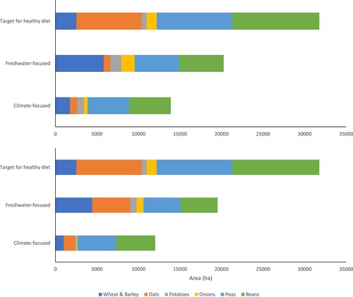
New Zealand does not currently produce enough of the right food for the prescribed and optimsed healthy diet. Not accounting for rotations, areas required to meet this healthy diet were 2522 ha wheat and barley, 7860 ha oats, 610 ha potatoes, 1210 ha onions, 9060 ha peas and 10508 ha beans above that currently produced for each of these crops (Table 1). Production targets were not met for all crops within the pressure catchments in either scenario (Figure 2). The deficit was grown outside the pressure catchments by replacing land use in suitable areas with crops that were more profitable (Table 1). However, a small deficit of 10% for citrus remained from a lower availability of suitable land for these crops (Table 1). Hence, to maintain the healthy diet, these deficits would have to be filled by imported food. Alternatively, the optimised diet could be reformulated to account for this constraint, which might allow New Zealand to produce a healthy diet completely domestically.

Figure 2. Areas (ha) of different crops grown for both scenarios in catchments under pressure for nitrogen (top) and phosphorus (bottom). Note that these data are not adjusted for rotations. For example, a crop may only be grown in one out of four years and require times the area to meet targeted yield. Total cropland in catchments under N pressure for the climate and freshwater-focused scenarios were 37,693 and 46,862 ha, respectively, while areas under P pressure were 34,671 and 45,763 ha, respectively. To adjust individual crop areas to account for their production within a rotation across New Zealand, areas outside of pressure catchments can be adjusted for wheat and barley, oats, potatoes, onions, peas and beans by dividing by 0.355, 0.37, 0.30, 0.43, 0.43 and 0.33, respectively.

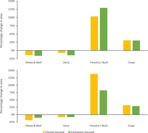
Nationally, land use change after accounting for target and non-target crops in rotations in order to decrease GHG emissions and water quality pressure amounted to an increase in cropland of 29-32% (on land suitable for cropping) and of 82-138% for forestry (on land not suitable for cropping). To accommodate this expansion of cropland and forestry, land in sheep and beef decreased by 11-19%, while land used for dairying decreased between 7-14% (Figure 3). Again, there was variation in these broad land use classes between N and P pressure catchments reflecting how much, for instance, class 6 and 7 land was present.

Figure 3. Percentage change across New Zealand in sheep and beef, dairy, forestry, and crops (adjusted for non-target crops in region-specific rotations) from current areas under both scenarios when focused on reducing nitrogen (top) or phosphorus (bottom). Current areas in sheep and beef, dairy, forestry, and cropland are 11.27, 2.24, 1.61, and 0.33 M ha, respectively.

Environmental performance

Within catchments under N pressure, the implementation of land use change in the climate- and freshwater-focused scenarios decreased N loss by 17.7 and 43.6%, respectively (Table 3). Within the P pressure catchments, land use changes decreased P losses in the climate- and freshwater-focused scenarios by 34.6 and 55.1%, respectively. Co-benefits of decreasing the non-target nutrient in a pressure catchment, for instance N in the P pressure catchments, were substantial, but generally less than for the targeted nutrient. For instance, P reductions in the N pressure catchments were 31.8 and 50.2% in the climate- and freshwater-focused catchments. The exception was a similar reduction in N load in the P pressure catchments in the climate-focused scenario (Table 3).

Table 3. Effect of each scenario on the non-optimised percentage change in nitrogen and phosphorus load, greenhouse gas emissions and gross margin, in catchments under pressure from nitrogen and phosphorus and when these data are scaled up (along with land use changes outside pressure catchments) to the national level focusing on N or P. Values in parentheses are the standard error calculated from regional values.

Area and scenario	Nitrogen load	Phosphorus load	Greenhouse gas emissions	Gross margin
N pressure catchments only
Climate focused	−17.7 (3.0)	−31.8 (4.3)	−535 (408)	1.3 (4.3)
Freshwater focused	−43.6 (5.3)	−50.2 (6.7)	−566 (302)	−8.9 (7.6)
P pressure catchments only
Climate focused	−20.9 (3.1)	−34.6 (4.6)	−824 (113)	0.5 (4.5)
Freshwater focused	−35.3 (6.0)	−55.1 (7.4)	−369 (132)	−8.3 (8.3)
National – N focus
Climate focused	−6.0 (1.6)	−9.9 (2.3)	−260 (176)	0.4 (1.7)
Freshwater focused	−12.7 (2.5)	−12.9 (2.8)	−336 (205)	−2.4 (2.6)
National – P focus
Climate focused	−7.1 (2.0)	−12.3 (3.1)	−348 (238)	0.2 (2.6)
Freshwater focused	−6.1 (1.7)	−9.7 (2.2)	−183 (59)	−1.4 (1.2)

When scaled to the national level, including land use outside of pressure catchments, N and P losses decreased between 6.0 and 12.9%. Interestingly, P losses decreased by 12.9% in the freshwater scenario when focusing on reducing N, presumably as these catchments were also nationally accounting for a disproportionately large amount of P loss (Table 3).

Land use change caused substantial decreases in GHG emissions associated with an increase in forestry. A much greater percentage reduction in GHG emissions occurred in the climate-focused scenario than the freshwater-focused scenario in the catchments under P pressure (Table 3). Reductions were slightly greater for the freshwater-focused scenario in N pressure catchments. This arose from less converson to forestry in the freshwater-focused scenario in N pressure catchments (Figure 3) and the reliance of suitable cropland being planted outside of the P pressure catchments.

The percentage gross margin was improved within both pressure catchments and when scaled up nationally under the climate-focused scenario but decreased under the freshwater-focused scenario (Table 3).

Land use changes in pressure catchments translated into a net loss of $1.29 to $1.90B for the sheep and beef sector and loss of $0.70 to $1.47B for the dairy sector. However, when profits from cropland and forestry were accounted for, gross margin ranged from a loss of $526M to a profit of $89M (Table 4).

Table 4. Effect of land use change on absolute ($M) gross margin in pressure catchments focusing on N or P.

Scenario	Cropland	Dairy	Sheep and Beef	Forestry	Sum difference
N focus
Climate focused	158	−702	−1,288	1,921	89
Freshwater focused	144	−1,466	−1,607	2,402	−526
P focus
Climate focused	155	−786	−1,897	2,571	42
Freshwater focused	145	−744	−1,242	1,526	−315

Regional effects

Amongst regions, large reductions in both N and P losses were noted in N and P pressure catchments for the Southland, Otago, Canterbury, Wellington, Manawatu-Wanganui, Hawkes Bay, and Waikato regions (Figures 4 and 5). The same inter-regional contrasts held for the magnitude of these percentage reductions but was attenuated when all land was considered within a region (see Supplementary Figures S6 and S7). When converted to absolute losses the greatest reductions within pressure catchments occurred in Canterbury, Manawatu-Wanganui, and Waikato regions (see Supplementary Data).

Figure 4. Effect of each scenario on the percentage change in nitrogen and phosphorus load, greenhouse gas emissions and gross margin in catchments under pressure from nitrogen in each region. The least significant difference at the P < 0.05 level is given for the contrast of regional means for both scenarios. Values refer to absolute estimated change in gross margin (millions NZD). Note that some decreases in greenhouse gas emissions exceed the y-axis scale.

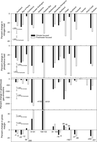
Figure 5. Effect of each scenario on the percentage change in nitrogen and phosphorus load, greenhouse gas emissions and gross margin in catchments under pressure from phosphorus in each region. The least significant difference at the P < 0.05 level is given for the contrast of regional means for both scenarios. Values refer to absolute estimated change in gross margin (millions NZD).

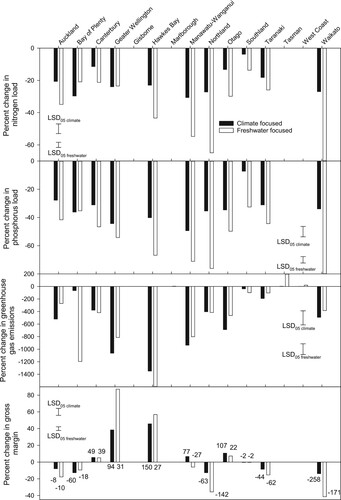
Many regions saw substantial percentage decreases in GHG emissions, but because of its large size and extent of pressure catchments, Canterbury saw the greatest absolute reductions. However, Manawatu-Wanganui saw the greatest absolute reductions in the climate-focused scenario, probably owing to a large amount of land in LUC class 6 and 7 that was converted to forestry (see Supplementary data).

Owing to the large areas of dairy land that was converted, gross margin was decreased in Waikato more than any other region across both scenarios within pressure catchments (Figures 4 and 5) and when scaled to the regional level (Supplementary Figures S6 and S7). However, because of the different areas and land uses present in Canterbury under N and P pressure, gross margin in the pressure catchments under a freshwater-focused scenario varied from a decrease of $288M in N pressure catchments to an increase of $39M in P pressure catchments (Figures 4 and 5). Under a climate-focused scenario, Canterbury had an increase in gross margin of $58 to $49M for catchments under N and P pressure, respectively owing to changes in sheep and beef land to forestry (Figures 4 and 5). National maps of land use change under both scenarios are also available in Supplementary Figures S8 and S9. Note that Gisborne, Tasman, and the West Coast had only small areas (<1% of the region) suitable for land use change (e.g. classified as Dairy C) near to processing faclities within catchments under pressure. Hence, these regions were excluded from optimisation to grow crops to meet the healthy diet in catchments under pressure. However, we did include these regions in our calculation to grow crops to meet the healthy diet outside of pressure catchments.

Discussion

Our aim was to determine if an optimised healthy diet could be grown in New Zealand, placing an emphasis on changing to the most suitable land in areas most likely to change. It can, but this varies depending on the scenario and which pressure catchments are assessed. There is also the potential for increased cost, but it is useful to put these costs into context. First, the highest modelled loss in gross margin at a national level of $526M is about 1% of the expected export revenues for the primary sector of $50.8B in the year to June 2022 (Ministry for Primary Industries 2021).

Internationally, much recent research has highlighted a link between an increase in the consumption of meat, cooking oils and non-starchy foods with an increase in GHG emissions and N and P losses to water (He et al. 2018). Globally, GHG emissions are estimated to be approximately 35–50% lower in ovolactovegetarian and vegan diets, respectively (Fresán and Sabaté 2019), while a water quality target of 1 mg L⁻¹ could be achieved across China if nutrient recycling rates increased from 36 to 87% (Yu et al. 2019). However, because pollution is high in China, achieving this target was estimated to have a capital cost of $100B USD with an annual cost of $18 to $29B USD (Yu et al. 2019). Amongst industrialised nations, water pollution in New Zealand is low (McDowell et al. 2020), while many mitigation options exist to reduce N and P losses (McDowell et al. 2018). This means that an array of cost-effective mitigation actions can be found and matched to combinations of catchment by land use resulting in lower costs on a per hectare basis than many other jurisdictions who have fewer, less cost-effective, options (McDowell et al. 2014). Our analysis therefore suggests that New Zealand has greater potential than many other countries to grow a healthy diet while minimising environmental and economic costs associated with land use change. Not only would such changes have potential to benefit New Zealander’s health and environment, they may also serve to support environmental credentials that aim to capture price premiums for exported produce before competitors (see also Implications section).

Limitations

Our modelling makes several assumptions and uses data which can inform the debate of national policy but should not be used to direct land use change at catchment scales. This recommendation arises from the coarse spatial scale of the available data which may make broad suitability of some crops invalid at finer scales (e.g., the ability to produce high quality milling wheat), potential inaccuracies in the tonnage or proxies for commodity crops that arise through changing annual production, and a static approach that did not consider flow paths or lag times between land use change and freshwater loads and concentrations.

In a little more detail, N and P pressure maps were produced at the catchment (often reach) scale. This assumes that if more than one farm is present, they are contributing to losses in proportion to their area. However, variation in climate, catchment conditions and farm management mean that N and P losses and GHG emissions will vary from the average types used here. Furthermore, the potential for N and P loss decreases the farther a farm is from the receiving environment (Macintosh et al. 2018). This occurs through processes such as attenuation that remove N and P by denitrification and sorption or settling-out or filtration of particles and often results in lag times between losses and the receiving waterbody that vary across a catchment (Van Meter and Basu 2017). We could not account for these processes in our optimisation of land use locations in every catchment owing to the computational power required and because data for attenuation is only available in a few locations. However, to mitigate their influence, we choose to optimise land use for fourth order streams, commensurate with the smallest scale at which Regional Authorities would likely mange land use and assumed that our estimates are relevant for 2035. This date accounts for the rate of agricultural innovation uptake which can vary from 6–23 years in Australasia (Botha et al. 2015; Kuehne et al. 2017) and lag times between land use change and surface water bodies in large catchments which have been estimated to be frequently <10 years (McDowell et al. 2021).

Another important source of potential error is a mismatch between the commodity crops modelled and the broad food groups they represent. Error here comes in two forms. The first is that the commodity is only a minor component of the broad food group. The second is that the commodity chosen had to be replaced by an ill-matched proxy. To alleviate both sources of error we matched commodities to broad food groups based on ingredient lists of the most popular food brands in the group and then checked whether these commodities could be grown and if not then chose a suitable proxy based on the work of Thomas et al. (2020). This work was checked by both growers and representatives from the arable and horticultural industries. However, additional work should also be done to determine if crops can be grown locally and matched to an appropriate supply and value chain.

Implications

An optimised healthy diet can be grown in New Zealand but utilises different areas when grown under a climate- and freshwater-focused scenario. Much of this was caused by our use of suitability mapping and the location of catchments under water quality pressure from N or P inputs. However, it is important to reiterate that our choice to let all land in class 6 and 7 change to forestry goes beyond the additional 570,000-760,000 ha proposed by the Climate Commission to meet the Government’s 2050 target (Climate Change Commission 2021). We did this to see if forestry, on land which can be poorly profitable, could result in lower N and P losses – thereby benefiting freshwater. It did, but depending on whether these were in N or P pressure catchments, additional reductions in N and P loads of 14-26% were required to meet the bottom line for algal growth in freshwaters (Table 3).

Reductions in N and P loads to meet the bottom lines for algal growth (freshwater-focused scenario) were larger than the climate-focused scenario and led to losses in gross margin compared to current values (Table 3). These losses were estimated to be up to $1.6B for the sheep and beef sector and $1.5B for the dairy sector in pressure catchments. These values contrast with the $6B loss estimated by the dairy sector in meeting nutrient limit (DairyNZ 2019). However, when other land uses were accounted for, losses in the freshwater scenario ranged from $315M to $526M (Table 3). These losses were closer to the $190M benefit estimated by the Government (Ministry for the Environment 2020b). The Ministry’s estimate (and our estimate) included income from land use change which DairyNZ excluded (Ministry for the Environment 2020b). However, it is important to note that our estimate was leveraged by forestry returns (of up to $2.4B). Concern has been raised over the proliferation of land use change from sheep and beef land to forestry (Yule 2022). This change is driven by greater returns for carbon sequestration but has begun to lock land into rotations of 20–30 years causing communities to wither as fewer people and their families are required to tend plantations. Additional concern has been raised over the aesthetics of plantation forestry. This has been somewhat alleviated by the realisation that about 20% of the 92,118 ha planted from 2017–2020 has been into manuka or native production forestry (Orme and Orme 2021). While manuka and native trees are likely to have similar N and P losses to exotic production forestry (Baillie and Neary 2015), the economic return from native trees, in particular totara, is limited to warmer regions where growth is quicker (Satchell 2021). Returns from manuka plantations are also variable depending on the quality of the honey produced (McPherson 2016). Even if the return from manuka/native forestry is half that of exotic plantation, at the current rate of planting (20%), the potential loss in revenue is far below the $14-20B cost savings estimated in the health care system from the consumption of the healthy diet (Drew et al. 2020). Hence, when the health of our people and environment are considered together, there is likely to be a net benefit from land use change.

Looking at exports, the reduction in sheep/beef and dairy land is 11-19%; however, as noted by the Climate Change Commission (2021) such a reduction may not impact on exports if improvements in productivity through genetic gain and farm management can be made on the remaining land. Genetic gain increases the feed conversion efficiency, with less feed required for animal maintenance and more feed converted into product. Evidence of gains already exist from both sectors. Mackay et al. (2012) noted that from 1989/90–2009/10 saleable product in the sheep and beef sector has increased 47% ha⁻¹ despite the area in sheep and beef shrinking from about 12 M ha in 1990/91–8. M ha in 2010/11 (Journeaux et al. 2017). Over this time, nitrate leaching and GHG emissions have decreased 21 and 40% per saleable product, respectively. In the dairy sector, land area has expended from 1.3M to 2.1 M ha (Journeaux et al. 2017), but productivity increased from 588 kg milk solids ha⁻¹–920 kg milk solids ha⁻¹ (DairyNZ 2015).

Conclusions

The modelling exercise presented here has connected a healthy diet, agricultural land use and environmental impacts for New Zealand in an integrated analysis. It has shown that shifting productive land uses to support a healthy, domestically produced diet for the New Zealand population can support meeting environmental targets for GHGs, N and P. The maximum cost of these changes is about 1% of the primary sector’s export revenues, and orders of magnitude less than the estimated savings for the health system from an optimised diet. Considered as an agri-food system, the country can improve its health and its environment while saving money.

Acknowledgements

We are grateful to Horticulture New Zealand and the Foundation for Arable Research in providing data on crop performance.

Disclosure statement

No potential conflict of interest was reported by the author(s).

Data availability statement

The supplementary data that support the findings of this study are openly available in figshare at https://doi.org/10.6084/m9.figshare.16614124.

Correction Statement

This article has been corrected with minor changes. These changes do not impact the academic content of the article.

Additional information

Funding

Funding for the paper was received through the Our Land and Water and Healthier Lives National Science Challenges from the Ministry of Business, Innovation and Employment (contracts: C10X1507 and UOOX1902, respectively).

Notes

1 https://manaakiwhenua.github.io/LUMASS

References

- Andersen LS, Gaffney O, Lamb W, Hoff H, Wood A. 2020. A safe operating space for New Zealand/Aotearoa: translating the planetary boundaries framework. [accessed 1 April, 2022]:[69 p.]. https://environment.govt.nz/assets/Publications/Files/a-safe-operating-space-for-nz-aotearoa.pdf.
- Baillie BR, Neary DG. 2015. Water quality in New Zealand’s planted forests: a review. N Z J For Sci. 45(1):7.
- Barber A, Pellow G, Barber M. 2011. Carbon footprint of New Zealand arable production - wheat, maize silage, maize grain and ryegrass seed. MAF Technical Paper No: 2011/97. [accessed 13 August, 2022]:[68 p.]. https://www.mpi.govt.nz/dmsdocument/4018/direct.
- Berkelaar M. 2007. LP solve: Opern Source (Mixed-Integer) Linear Programming System (2007). http://lpsolvesourceforgenet/55/.
- BERL. 2022. Economic impact 2021. Arable Food Industry Council. [accessed 2022 Sep]. https://www.afic.co.nz/wp-content/uploads/2022/07/AFIC-Economic-Impact-2021.pdf.
- Botha N, Turner JA, Sinclair S, Brazendale R, Dirks S, Blackett P, Lambert G. 2015. Assessing the economic impact of a co-innovation approach: the case of dairy heifer rearing in New Zealand. ImpAR Conference 2015 Impacts of agricultural research - towards an approach of societal; 3-4 November, 2015; Pairs, France.
- Cleghorn C, Nghiem N, Ni-Mhurchu C. 2022a. New Zealand diet optimised for health, cost and climate protection. Sustainable Healthcare and Climate Health Aotearoa conference; Wellington, New Zealand.
- Cleghorn C, Nghiem N, Ni-Mhurchu C. 2022b. Assessing the health and environmental benefits of a New Zealand diet optimised for health and climate protection. Sustainability. In press.
- Climate Change Commission. 2021. Ināia tonu nei: a low emissions future for Aotearoa. [accessed 13 August, 2022]:[418 p.]. https://ccc-production-media.s3.ap-southeast-2.amazonaws.com/public/Inaia-tonu-nei-a-low-emissions-future-for-Aotearoa/Inaia-tonu-nei-a-low-emissions-future-for-Aotearoa.pdf.
- Cooper AB, Thomsen CE. 1988. Nitrogen and phosphorus in streamwaters from adjacent pasture, pine, and native forest catchments. N Z J Mar Freshwat Res. 22:279–291.
- Curtin D, Hanson R, Van Der Weerden TJ. 2008. Effect of selenium fertiliser formulation and rate of application on selenium concentrations in irrigated and dryland wheat (Triticum aestivum). N Z J Crop Hortic Sci. 36(1):1–7.
- DairyNZ. 2015. 2014/15 New Zealand Dairy Statistics. [accessed 13 September, 2016]. https://www.dairynz.co.nz/publications/dairy-industry/new-zealand-dairy-statistics-2014-15/.
- DairyNZ. 2019. Action for healthy waterways: DairyNZ submission. [accessed 6 March, 2020]:[236 p.]. https://www.dairynz.co.nz/media/5792331/dairynz-ef-submission.pdf.
- Davis M. 2014. Nitrogen leaching losses from forests in New Zealand. N Z J For Sci. 44(1):2.
- Drew J, Cleghorn C, Macmillan A, Mizdrak A. 2020. Healthy and climate-friendly eating patterns in the New Zealand context. Environ Health Perspect. 128(1):017007.
- Evans R. 2002. An alternative way to assess water erosion of cultivated land – field-based measurements: and analysis of some results. Applied Geography. 22(2):187–207.
- Fenemor A, Green S, Dryden G, Samarasinghe O, Newsome P, Price R, Betts H, Lilburne L. 2015. Crop production, profit and nutrient losses in relation to irrigation water allocation and reliability – Waimea Plains, Tasman District. [accessed 13 August, 2022]:[73 p.]. https://www.mpi.govt.nz/dmsdocument/9899/direct.
- Fertiliser Association of New Zealand. 2018. Fertiliser Association of New Zealand. Wellington, New Zealand: Fertiliser Association of New Zealand; [accessed 2018 September]. http://www.fertiliser.org.nz.
- Fresán U, Sabaté J. 2019. Vegetarian diets: planetary health and its alignment with human health. Adv Nutr. 10(Supplement 4):S380–S388.
- Gustavsson J, Cederberg C, Sonesson U, van Otterdijk R, Maeybeck A. 2011. Global food and food waste. [accessed 14 September, 2021]:[37 p.]. http://www.fao.org/3/mb060e/mb060e00.htm.
- Harris S, McDowell RW, Lilburne L, Laurenson S, Dowling L, Guo J, Pletnyakov P, Beare M, Palmer D. 2021. Developing an indicator of productive potential to assess land use suitability in New Zealand. Environ Sustain Indic. 11:100128.
- He P, Baiocchi G, Hubacek K, Feng K, Yu Y. 2018. The environmental impacts of rapidly changing diets and their nutritional quality in China. Nat Sustain. 1(3):122–127.
- Herzig A, Ausseil A-G, Dymond JR. 2013. Spatial optimisation of ecosystem services. Ecosystem services in New Zealand – conditions and trends.[511-523 p.]. http://www.mwpress.co.nz/__data/assets/pdf_file/0005/77063/3_3_Herzig.pdf.
- Herzig A, Dymond J, Ausseil AG. 2016. Exploring limits and trade-offs of irrigation and agricultural intensification in the Ruamahanga catchment, New Zealand. N Z J Agric Res. 59(3):216–234.
- Herzig A, Nguyen TT, Ausseil A-GE, Maharjan GR, Dymond JR, Arnhold S, Koellner T, Rutledge D, Tenhunen J. 2018. Assessing resource-use efficiency of land use. Environ Model Softw. 107:34–49.
- Hutchinson K, Rennie G, Vibart R, Mercer G, O'Neil K, Burtt A, Chrystal J, Devantier B, Smiley D, Taylor A, et al. 2019. Greenhouse gas emissions from New Zealand sheep-and-beef farm systems. N Z J Sci Product. 79:56–60.
- Journeaux P, van Reenan E, Manjala T, Pike S, Hanmore I, Millar S. 2017. Analysis of drivers and barriers to land use change. [accessed 12 August, 2022]:[90 p.]. https://www.mpi.govt.nz/dmsdocument/23056/direct.
- KPMG. 2017. Agribusiness agenda 2017: the recipe for action. https://home.kpmg.com/content/dam/kpmg/nz/pdf/June/agri-agenda-2017-kpmg-nz.pdf.
- Kuehne G, Llewellyn R, Pannell DJ, Wilkinson R, Dolling P, Ouzman J, Ewing M. 2017. Predicting farmer uptake of new agricultural practices: a tool for research, extension and policy. Agric Syst. 156:115–125.
- Landcare Research. 2017. NZ Land Cover Database. Lincoln, New Zealand: Landcare Research: Manaaki Whenua; [accessed 2018 11 April]. http://www.lcdb.scinfo.org.nz/home.
- Livestock Improvement Corporation Limited, DairyNZ. 2019. New Zealand Dairy Statistics 2018-19. [accessed 13 August, 2022]:[60 p.]. https://www.dairynz.co.nz/media/5792471/nz_dairy_statistics_2018-19_web_v2.pdf.
- Lynn IH, Manderson AK, Page MJ, Harmsworth GR, Eyles GO, Douglas GB, Mackay AD, Newsome PJF. 2009. Land use capability survey handbook. A New Zealand handbook for the classification of land. 3rd ed. Hamilton: AgResearch, Landcare Research, GNS Science. http://www.landcareresearch.co.nz/publications/books/luc.
- Macintosh KA, Mayer BK, McDowell RW, Powers SM, Baker LA, Boyer TH, Rittmann BE. 2018. Managing diffuse phosphorus at the source versus at the sink. Environ Sci Technol. 52(21):11995–12009.
- Mackay AD, Rhodes AP, Power I, Wedderburn ME. 2012. Has the eco-efficiency of sheep and beef farms changed in the last 20 years? Proc N Z Grass Assoc. 74:11–16.
- Mazzetto A, Falconer S, Ledgard S. 2021. Mapping the carbon footprint of milk for dairy cows. [accessed 20 August 2021]:[25 p.]. https://www.dairynz.co.nz/media/5794083/mapping-the-carbon-footprint-of-milk-for-dairy-cows-report-updated.pdf.
- McDowell RW, Moreau P, Salmon-Monviola J, Durand P, Leterme P, Merot P. 2014. Contrasting the spatial management of nitrogen and phosphorus for improved water quality: modelling studies in New Zealand and France. Eur J Agron. 57:52–61.
- McDowell RW, Noble A, Pletnyakov P, Haggard BE, Mosley LM. 2020. Global mapping of freshwater nutrient enrichment and periphyton growth potential. Sci Rep. 10(1):3568.
- McDowell RW, Schallenberg M, Larned S. 2018. A strategy for optimizing catchment management actions to stressor–response relationships in freshwaters. Ecosphere. 9(10):e02482.
- McDowell RW, Simpson ZP, Ausseil AG, Etheridge Z, Law R. 2021. The implications of lag times between nitrate leaching losses and riverine loads for water quality policy. Sci Rep. 11(1):16450.
- McDowell RW, Snelder T, Harris S, Lilburne L, Larned ST, Scarsbrook M, Curtis A, Holgate B, Phillips J, Taylor K. 2018. The land use suitability concept: introduction and an application of the concept to inform sustainable productivity within environmental constraints. Ecol Indicators. 91:212–219.
- McDowell RW, Wilcock RJ. 2008. Water quality and the effects of different pastoral animals. N Z Vet J. 56(6):289–296.
- McNeill SJE, Golubiewski N, Barringer J. 2014. Development and calibration of a soil carbon inventory model for New Zealand. Soil Res. 52(8):789–804.
- McPherson A. 2016. Manuka – a viable alternative land use for New Zealand’s hill country? N Z J Forest. 61(3):11–19.
- Ministry for Primary Industries. 2017. 2017 Pipfruit Monitoring Programme. [accessed 13 August, 2022]:[4 p.]. https://www.mpi.govt.nz/dmsdocument/26506-farm-monitoring-report-2017-pipfruit-monitoring-programme.
- Ministry for Primary Industries. 2021. Situation and Outlook for Primary Industries. [accessed 6 March, 2022]:[43 p.]. https://www.mpi.govt.nz/resources-and-forms/economic-intelligence/situation-and-outlook-for-primary-industries/sopi-reports/.
- Ministry for the Environment. 2020a. National Policy Statement for Freshwater Management 2020. [accessed 11 August, 2022]:[70 p.]. https://www.mfe.govt.nz/sites/default/files/media/Fresh%20water/national-policy-statement-for-freshwater-management-2020.pdf.
- Ministry for the Environment. 2020b. Overview of the impact analysis undertaken to inform decisions on freshwater policy, with a focus on monetised costs. [accessed 6 June, 2020]:[14 p.]. https://www.mfe.govt.nz/sites/default/files/media/Fresh%20water/overview-of-impact-analysis-undertaken-to-inform-decisions-freshwater-policy.pdf.
- Ministry for the Environment. 2021. New Zealand's Greenhouse Gas Inventory 1990-2019. [accessed 9 September, 2022]:[531 p.]. https://environment.govt.nz/assets/Publications/New-Zealands-Greenhouse-Gas-Inventory-1990-2019-Volume-1-Chapters-1-15.pdf.
- Ministry for the Environment, Statistics New Zealand. 2020a. Agricultural and horticultural land use. Wellington, New Zealand: Statistics New Zealand; [accessed 2020 11 November]. http://infoshare.stats.govt.nz/browse_for_stats/environment/environmental-reporting-series/environmental-indicators/Home/Land/land-use.aspx.
- Ministry for the Environment, Statistics New Zealand. 2020b. Our Freshwater 2020. [accessed 13 August, 2022]:[94 p.]. https://environment.govt.nz/assets/Publications/Files/our-freshwater-2020.pdf.
- Ministry of Health. 2020. Eating and activity guidelines for New Zealand adults: updated 2020. [accessed 13 August, 2022]:[164 p.]. https://www.health.govt.nz/system/files/documents/publications/eating-activity-guidelines-new-zealand-adults-updated-2020-jul21.pdf.
- Monaghan R, Manderson A, Basher L, Smith C, Burger D, Meenken E, McDowell RW. 2021. Quantifying contaminant losses to water from pastoral landuses in New Zealand I. Development of a spatial framework for assessing losses. N Z J Agric Res. 64(3):344–364.
- New Zealand Government. 2019. Climate Change Response (Zero Carbon) Amendment Act 2019. Public Act 2019 No 61. [accessed 13 August, 2022]:[32 p.]. http://www.legislation.govt.nz/act/public/2019/0061/latest/096be8ed8190b20c.pdf.
- Norris M, Johnstone P, Liu J, Arnold N, Sorenson I, Green S, van den Djissel C, Dellow S, Wright P, Clark G. 2019. Rootzone reality: technical review on network performance. [accessed 3 March 2021]:[66 p.]. https://www.vri.org.nz/dmsdocument/192-16576-matthew-norris-rootzone-reality-technical-review-on-network-final2.
- Oehler F, Elliott AH. 2011. Predicting stream N and P concentrations from loads and catchment characteristics at regional scale: a concentration ratio method. Sci Total Environ. 409(24):5392–5402.
- Orme S, Orme P. 2021. Independent validation of land-use change from pastoral farming to large-scale forestry. [accessed 29 March, 2022]:[38 p.]. https://beeflambnz.com/sites/default/files/Potential-land-use-change-pasture-to-forest-species-report.pdf.
- Plant and Food Research. 2019. Fresh facts: New Zealand horticulture 2019. [accessed 13 August, 2022]:[23 p.]. https://www.freshfacts.co.nz/files/freshfacts-2019.pdf.
- Poore J, Nemecek T. 2018. Reducing food’s environmental impacts through producers and consumers. Science. 360(6392):987–992.
- Rajaniemi M, Mikkola H, Ahokas J. 2011. Greenhouse gas emissions from oats, barley, wheat and rye production. Agron Res. 9:189–194.
- Reynish R. 2020. Financial budget manual gross margins 2020. Lincoln: Lincoln University.
- Roth GA, Abate D, Abate KH, Abay SM, Abbafati C, Abbasi N, Abbastabar H, Abd-Allah F, Abdela J, Abdelalim A, et al. 2018. Global, regional, and national age-sex-specific mortality for 282 causes of death in 195 countries and territories, 1980–2017: a systematic analysis for the Global Burden of Disease Study 2017. The Lancet. 392(10159):1736–1788.
- Rush E, Obolonkin V. 2020. Food exports and imports of New Zealand in relation to the food-based dietary guidelines. Eu J Clin Nutr. 74(2):307–313.
- Ryden JC, Syers JK, Harris RF. 1973. Phosphorus in runoff and streams. Adv Agron. 25:1–45.
- Sanson R. 2005. The AgribaseTM farm location database. Proceedings of the New Zealand Society of Animal Production. 65(93–96).
- Satchell D. 2021. Land Use Options and Economic returns for Marginal Hill Country in Northland. [accessed 30 March, 2022]:[19 p.]. https://www.nrc.govt.nz/media/maylldkj/land-use-options-and-economic-returns-for-marginal-hill-country-in-northland-final-a1412777.pdf.
- Saunders C, Barber A, Taylor G. 2006. Food miles – comparative energy/emissions performance of New Zealand’s agriculture industry. Christchurch: Agribusiness & Economics Research Unit, Lincoln University. http://hdl.handle.net/10182/125.
- Saunders C, Dalziel P, Guenther M, Saunders J, Rutherford P. 2016. The land and the brand. [accessed 22 May 2022]:[127 p.]. https://researcharchive.lincoln.ac.nz/bitstream/handle/10182/6920/AERU%20RR%20339%20Land%20and%20the%20Brand%20Report.pdf?sequence = 3.
- Snelder TH, Moore C, Kilroy C. 2019. Nutrient concentration targets to achieve periphyton biomass objectives incorporating uncertainties. JAWRA J Amer Water Resour Assoc. 55(6):1443–1463.
- Statistics New Zealand. 2018. Agriculture, horticulture, and forestry. Wellington, New Zealand: Statistics New Zealand; [accessed 2018 8 October]. http://archive.stats.govt.nz/browse_for_stats/industry_sectors/agriculture-horticulture-forestry.aspx.
- Statistics New Zealand. 2021. New Zealand's greenhouse gas emissions. Wellington, New Zealand: Statistics New Zealand; [accessed 2021 20 August]. https://www.stats.govt.nz/indicators/new-zealands-greenhouse-gas-emissions.
- Steinfield H, Gerber P, Wassenaar T, Castel V, Rosales M, de Haan C. 2006. Livestock's long shadow: environmental issues and options. Rome, Italy.
- Swain M, Blomqvist L, McNamara J, Ripple WJ. 2018. Reducing the environmental impact of global diets. Sci Total Environ. 610-611:1207–1209.
- Thomas S, Ausseil A-G, Guo J, Herzig A, Khaembah EN, Palmer D, Renwick A, Teixeira E, van der Weerden T, Wakelin SJ. 2020. Evaluation of profitability and future potential for low emission productive uses of land that is currently used for livestock Wellington, New Zealand.
- Tsushima K, Koike T, Horinouchi Y, Inoue T, Yamada T. 2009. Evaluation of nutrient loads from a citrus orchard in Japan. J Water Environ Technol. 7(4):267–276.
- University of Otago, Ministry of Health. 2011. A focus on nutrition: key findings of the 2008/09 New Zealand Adult Nutrition Survey. Wellington, New Zealand.
- Van der Weerden T, Beukes P, De Klein C, Hutchinson K, Farrell L, Stormink T, Romera A, Dalley D, Monaghan R, Chapman D, et al. 2018. The effects of system changes in grazed dairy farmlet trials on greenhouse gas emissions. Animals. 8(12):234.
- Van Meter KJ, Basu NB. 2017. Time lags in watershed-scale nutrient transport: an exploration of dominant controls. Environ Res Lett. 12(8):084017.
- Wang Y, Sharp B, Poletti S, Nam K-M. 2021. Economic and land use impacts of net zero-emission target in New Zealand. Intern J Urban Sci. (Jan):291–308. https://doi.org/10.1080/12265934.2020.1869582.
- Yu C, Huang X, Chen H, Godfray HCJ, Wright JS, Hall JW, Gong P, Ni S, Qiao S, Huang G, et al. 2019. Managing nitrogen to restore water quality in China. Nature. 567(7749):516–520.
- Yule L. 2022. Managing firestry land-use under the influence of carbon: the issues and options. [15 p.]. https://beeflambnz.com/sites/default/files/news-docs/Green-Paper-Managing%20Forestry-Land-Use%20-Carbon.pdf.