The role of governmental weapons procurements in forecasting monthly fatalities in intrastate conflicts: A semiparametric hierarchical hurdle model

Abstract

Accurate and interpretable forecasting models predicting spatially and temporally fine-grained changes in the numbers of intrastate conflict casualties are of crucial importance for policymakers and international non-governmental organizations (NGOs). Using a count data approach, we propose a hierarchical hurdle regression model to address the corresponding prediction challenge at the monthly PRIO-grid level. More precisely, we model the intensity of local armed conflict at a specific point in time as a three-stage process. Stages one and two of our approach estimate whether we will observe any casualties at the country- and grid-cell-level, respectively, while stage three applies a regression model for truncated data to predict the number of such fatalities conditional upon the previous two stages. Within this modeling framework, we focus on the role of governmental arms imports as a processual factor allowing governments to intensify or deter from fighting. We further argue that a grid cell’s geographic remoteness is bound to moderate the effects of these military buildups. Out-of-sample predictions corroborate the effectiveness of our parsimonious and theory-driven model, which enables full transparency combined with accuracy in the forecasting process.

Los modelos de previsión precisos e interpretables que predicen los cambios a nivel espacial y temporal en la cantidad de víctimas de los conflictos intraestatales son de vital importancia para los responsables políticos y las organizaciones no gubernamentales (ONG) internacionales. Utilizando un enfoque de datos de recuento, proponemos un modelo de regresión Hurdle jerárquico para abordar el correspondiente reto de predicción a nivel mensual de PRIO-GRID. Más concretamente, modelamos la intensidad del conflicto armado local en un momento determinado como un proceso de tres etapas. Las etapas uno y dos de nuestro enfoque estiman si observaremos alguna víctima a nivel de país y de celda de la red, respectivamente, mientras que la etapa tres aplica un modelo de regresión para datos truncados con el propósito de predecir la cantidad potencial de dichas víctimas mortales en función de las dos etapas anteriores. Dentro de este marco de modelización, nos centramos en el rol de las importaciones de armas por parte de los gobiernos como un factor de proceso que permite a los gobiernos intensificar o impedir los enfrentamientos. Además, sostenemos que la lejanía geográfica de una célula de la red está destinada a moderar los efectos de estas concentraciones militares. Las predicciones fuera de la muestra corroboran la eficacia de nuestro modelo parsimonioso y basado en la teoría, que permite una transparencia total combinada con precisión en el proceso de previsión.

Les modèles de prévision précis et interprétables, qui permettent de prédire spatialement et temporellement les détails des changements dans les nombres de victimes de conflits intra-étatiques, sont d’une importance cruciale pour les décideurs politiques et les organizations non gouvernementales (ONG) internationales. Nous adoptons une approche par données de comptage et nous proposons un modèle de régression hiérarchique à obstacle (hurdle) pour relever le défi de la prédiction correspondante au niveau de la grille mensuelle du PRIO (Peace research institute Oslo, Institut de recherche sur la paix d’Oslo). Plus précisément, nous modélisons l’intensité des conflits armés locaux à un moment spécifique sous la forme d’un processus en trois étapes. Les étapes un et deux de notre approche consistent à estimer si nous observerons des pertes respectivement au niveau du pays et de la cellule de grille, tandis que l’étape trois consiste à appliquer un modèle de régression pour les données tronquées afin de prédire le nombre de ces pertes en fonction des deux étapes précédentes. Dans ce cadre de modélisation, nous nous concentrons sur le rôle des importations d’armes gouvernementales en tant que facteur processuel permettant aux gouvernements d’intensifier ou de dissuader les combats. Nous soutenons également que l’isolement géographique d’une cellule de la grille est susceptible de modérer les effets de ces renforcements militaires. Des prédictions hors échantillon corroborent l’efficacité de notre modèle parcimonieux fondé sur la théorie qui permet une totale transparence associée à une précision du processus de prévision.

Keywords:

• Conflict forecasting
• conflict intensity
• Forecasting
• hurdle regression
• semiparametric regression

View correction statement:

Correction

Introduction

Within sub-Saharan Africa alone, the violent deaths of close to 8,500 people are attributed to state-based armed conflict in 2019 (Pettersson and Öberg 2020). Reliable forecasts of conflict intensifications before they occur allow policymakers to take precautionary and de-escalatory measures, thus decreasing the human toll of organized violence. We present an approach that extends recent advances in the forecasting of armed conflicts (e.g., Blair and Sambanis 2020; Chiba and Gleditsch 2017; Hegre et al. 2019; Ward et al. 2013) toward forecasting conflict intensity, as indicated by the number of casualties resulting from state-based conflicts. We follow this endeavor at the geographically highly disaggregated level of the PRIO grid cell, which is a standardized structure introduced by Tollefsen, Strand, and Buhaug (2012) comprising quadratic grid cells that cover the entire world at an approximate resolution of 55 × 55 km. By doing so, we extend the current literature in two main regards. First, we propose to forecast the intensity of state-based fighting by employing a novel hierarchical hurdle regression model that we develop in accordance with our theoretic considerations. Second, we expand the suite of commonly used covariates to include the role of governmental weapons procurements on the country level.

Our model rests on the idea of hurdle models (Cragg 1971) but advances the corresponding model class in two main aspects: we incorporate three nested stages and adopt thresholding (Sheng and Ling 2006), a technique from cost-sensitive classification, to hurdle models. In this stage-wise regression, the first stage indicates whether we will observe any fatalities at the country level (country violence incidence). The second stage controls whether conditional on having any casualties at the country level, we will also observe a non-zero number of deaths in a given grid cell (cell violence incidence). Given that this is the case, the third stage then uses truncated regression to estimate the number of fatalities (cell violence intensity). To make predictions that are consistent with the training observations, we introduce two cutoff parameters that serve as thresholds known from cost-sensitive classifications in the first two binary stages of our model (Hernández-Orallo, Flach, and Ferri 2012). We set these parameters according to a metric that ensures well-calibrated predictions, i.e., predicting approximately the cumulative fatalities we observe.

In applying our three-staged approach to forecasting local conflict intensity, we heed recent calls for more theory-based conflict prediction (Blair and Sambanis 2020; Cederman and Weidmann 2017; Chiba and Gleditsch 2017) and limit the covariates in our model to a parsimonious set of theoretically motivated variables. In line with the suggestion to “focus on the processes that produce violence closer to the moment of onset” (Chiba et al. 2017, 3), we emphasize governmental major conventional weapons imports as a driver of conflict intensity (Mehrl and Thurner 2020). These transfers include large-scale weapons such as aircraft, artillery, or tanks,¹ and also increase the risk of violence to occur (Magesan and Swee 2018; Pamp et al. 2018). However, as we discuss below, their conflict-inducing effect will not be homogeneous across all locations within a country. In particular, we expect that governmental imports of major conventional weapons increase fighting intensity but that this effect decreases with a location’s distance from the capital. This is the case as remote localities are harder to reach for armies that employ major conventional weapons due to their lower ability to traverse rough terrain, increased reliance on road infrastructure, and more challenging logistics.

In support of our modeling approach, the out-of-sample evaluation indicates that our hierarchical hurdle regression model outperforms a competitive random forest benchmark model. Furthermore, our test results suggest that the inclusion of governmental arms imports increases the predictive accuracy of the forecasts. We will henceforth use the abbreviations PGM and CM when referring to monthly observations at the PRIO-grid and country level. The corresponding spatial units are shortened to PG (PRIO-grid cell) and C (country).

This article’s remainder is structured as follows: the next section motivates the hierarchical structure and use of a hurdle model in the application case. Building on this theoretical foundation, we then formally introduce the semiparametric hierarchical hurdle model. Subsequently, we apply this model to predict local conflict intensity at the PRIO grid level. This section also presents the specification of a parsimonious suite of covariates, out-of-sample evaluation results, as well as forecasts until March 2021. The paper concludes with a discussion of possible future directions.

Theoretical Motivation

A principal issue in modeling armed conflict is that conflict events are empirically rare. This is the case for all commonly used units of observation (state-dyads, country-years, etc.) but in particular at more granular levels of spatiotemporal resolution such as PGs. For instance, even throughout the Liberian civil war, most locations in Liberia did not experience any fighting as violence instead clustered in a few areas (Hegre, Østby, and Raleigh 2009). And while resulting in over 22,000 civilian casualties, much of the violence in the Bosnian civil war was concentrated in a few infamous events, most prominently the massacres in Srebrenica and Prijedor. In contrast, other periods passed without any reported killings of civilians (Schneider, Bussmann, and Ruhe 2012). The main concern here is that an excess of zero-observations exists, i.e. observations where no conflict occurs (Bagozzi 2015; Beger, Dorff, and Ward 2016). Most obviously, some country-pairs, states, or subnational locations may be as good as immune to armed conflict because of their particular wealth, institutional features, or geographical attributes. For instance, it is highly improbable that Djibouti and Lesotho would ever engage in a mutual dispute or that Liechtenstein would experience civil war. But even in countries with an ongoing conflict, fighting is usually geographically confined and unlikely to reach locations such as the capital (Buhaug 2010; Hegre, Østby, and Raleigh 2009; Tollefsen and Buhaug 2015). Furthermore, such excess zeroes can also occur temporally and, if left unaccounted for, threaten both inference and our ability to forecast fighting (Bagozzi 2015).

When predicting the monthly conflict intensity at the spatially highly disaggregated PRIO grid level, this discussion has relevant implications. To begin, we can expect that as numerous countries will be at peace in either a month under observation or even across the entirety of the period we study, none of the grid cells contained within them will experience any fighting. And even when violence does occur on the country-month level, the majority of its grid cells will nonetheless see no combat. A descriptive analysis of the available data, covering violence at the cell-month level across Africa during the period 1990–2019, supports these expectations. First, most fatalities occur in a small subset of countries that hardly changes over time.² This implies that hierarchical structure, i.e., in which country each cell is situated, carries vital information for the prediction task. Second, the vast majority of grid cells—even within countries experiencing combat—($99.2\mathrm{\%}$) are reporting zero cases. As there are more than 10,000 grid cells defined in Africa for each month, the datasets might therefore include up to 3,8 million observations. This, in turn, can posit an obstacle when estimating flexible and realistic models in a context where fast as well as precise and interpretable predictions are needed.

In predicting PGM-level fighting, we focus on the external procurement of major conventional weapons as a critical factor that allows governments to engage in and escalate armed conflict. Existing studies identify these imports as drivers of conflict onset (Magesan and Swee 2018; Pamp et al. 2018) but also emphasize their potential to intensify current fighting as they increase governmental forces’ ability to pin down the enemy and engage in decisive battles (Caverley and Sechser 2017; Mehrl and Thurner 2020). Hence, the procurement of weapons is a driver of both the occurrence and intensity of conflict. That being said, governmental arms imports are a country-level factor while we are interested in predicting grid-level fighting; this is particularly relevant as grid cells differ in terms of their potential to experience conflict or be exposed to government-owned heavy weaponry. Namely, the state’s reach—and hence rebels opportunity to challenge it—varies over its territory, with locations far away from the capital being the most difficult to govern and thus most suitable for rebellion (Boulding 1962; Buhaug 2010; Tollefsen and Buhaug 2015). Such remoteness may, in turn, mainly affect the power projection ability of forces employing major conventional weapons given their comparatively lower ability to traverse rough terrain, higher reliance on road infrastructure, and more challenging logistics. In addition to increasing the country-level occurrence and intensity of fighting, governmental arms imports may hence also determine combat severity at the more local level. We thus use the external procurement of weapons to identify which countries experience fighting and, in interaction term with a PG’s distance from the capital, to predict the local occurrence and intensity of violence within these countries. Additionally, we differentiate between the short- and long-term effects of these weapons as they may correspond to different theoretical mechanisms. Along these lines, MCW may increase the risk of short-term combat incidence as they allow a threatened incumbent to attack their challenger. But in the long-run, such weapon buildups may instead serve to deter to challengers, thus decreasing conflict risk (see Pamp et al. 2018). At the same time, for MCW imports to increase an incumbent’s ability to not just strike once against a challenger but to meaningfully intensify fighting, a period of distributing and training on these weapons will be necessary. As such, MCW imports may be expected to affect the intensity of combat mainly in the long run.

Hierarchical Hurdle Regression

Stemming from this discussion, we propose a forecasting model, which can incorporate the hierarchical data structure, given by each PG allocation in a country, as well as appropriately deal with the high rate of excess zeros. These aims are mirrored in two model characteristics: a stage-wise formulation and an application of cutoff values for prediction. Our model explicitly assumes that state-based PG fatalities occur only in countries that we predict to have at least one fatality. We make this prediction based on a binary regression model on the country level and introduce a cutoff value to obtain binary predictions. Given that this prediction forecasts fatalities on the country level, we progress to a second binary decision on the PG level to determine if we will observe at least one case in the respective cell. Similar to the first binary choice, we use an additional cutoff value to attain binary predictions. Provided that this binary result is again positive at the PGM level, we capture the realized count by a truncated distribution defined over the positive natural numbers.³

Model Formulation

For a precise notation, we order each grid cell according to the country it is situated in and, therefore, define $y_{ijt}$ to be the observed number of state-based fatalities in PRIO-grid $i$ situated in country $j$ and month $t,$ with $i=1,\dots ,n_j,$ $j=1,\dots ,n$ and $t\in \mathcal{T}=\{\mathrm{J}\mathrm{a}\mathrm{n}\mathrm{u}\mathrm{a}\mathrm{r}\mathrm{y}\mathrm{ }1990,\dots ,\mathrm{M}\mathrm{a}\mathrm{r}\mathrm{c}\mathrm{h}\mathrm{ }2021\}.$

In our application we set $n=55$ (number of countries) and $n_j$ denotes the number of cells located in country $j=1,\dots ,n.$ Since our model combines both the country and grid level, let $y_{\cdot jt}={\sum }_{i=1}^{n_j}{y}_{ijt}$ be the corresponding observation aggregated at the country level. In accordance with the abbreviations introduced earlier, we write CM $jt$ and PGM $ijt$ to shorten the corresponding observations. Further, we define a binarised version of $y_{\cdot jt}$ by ${\tilde{y}}_{\cdot jt},$ hence ${\tilde{y}}_{\cdot jt}=y_{\cdot jt}>0.$ Within this notation, the aim of the prediction task is to forecast ${\mathrm{\Delta }}_{ijt}^s$ defined by: (1) $$\text{log}\hspace{0.17em}(y_{\mathit{ijt}}+1)-\hspace{0.17em}\text{log}\hspace{0.17em}(y_{\mathit{ijt}-s}+1)\text{with}(t,s)\in \{(\text{October}2020,2),\dots ,(\text{March}2021,7)\},$$(1) with data given until $t-s.$ Since the sole stochastic component of (1) is $\text{log}(y_{ijt}+1)$ it suffices to model the observed counts at the point in time $t.$ We tackle this endeavor with six models that only differ by the assumed lag structure of $s$ months between the measurement of all covariates and the target variable (with $s=2,\dots ,7$). Since we have data until August 2020, the one-step-ahead forecasts of these models yield the predictions needed in (1). Simply put, the prediction of the time-step $s$ months into the future translates into a lag of $s$ months between covariates and the target variable. Without a loss of generality, we hence formulate our model for the arbitrary delay structure of $s$ months.

In our three-stage hurdle regression model, we decompose the probability distribution of the random variable $Y_{ijt}$ into two binary decisions and a truncated counting model. In stage 1 we start with a binary classification model on the country level in which the target variable is the random variable $Y_{\cdot jt},$ indicating whether we observed at least one fatality in CM $jt.$ Conditional on having observed at least one fatality in CM $jt,$ the consecutive two stages encompass a standard hurdle regression model (Mullahy 1986). Therefore, stage 2 constitutes another binary decision determining if we observe at least one fatality in PGM $ijt,$ while stage 3 models the count of deaths conditional on having observed at least one death in the respective cell. For stage 3, we utilize a truncated counting distribution. Mathematically, the resultant probability model of this stage-wise approach can be stated as the joint bivariate probability of $Y_{ijt}$ and ${\tilde{Y}}_{\cdot jt}$ with delay structure $s$ by: (2) $$\mathbb{P}(Y_{ijt}=y_{ijt},{\tilde{Y}}_{\cdot jt}={\tilde{y}}_{\cdot jt}|x_{\cdot jt-s}^{(1)},x_{ijt-s}^{(2)},x_{ijt-s}^{(3)})=\left\{\begin{array}{l}(1-{\pi }_{\cdot jt}^{(1)}){\tilde{y}}_{\cdot jt}=0,y_{ijt}=0\\ {\pi }_{\cdot jt}^{(1)}(1-{\pi }_{ijt}^{(2)}){\tilde{y}}_{\cdot jt}=1,y_{ijt}=0\\ {\pi }_{\cdot jt}^{(1)}{\pi }_{ijt}^{(2)}{f}_{tr}^{(3)}(y_{ijt}){\tilde{y}}_{\cdot jt}=1,y_{ijt}>0\\ 0\mathrm{e}\mathrm{l}\mathrm{s}\mathrm{e}\end{array}\right.,$$(2) where ${\pi }_{\cdot jt}^{(1)}$ is the probability of observing at least one fatality in CM $jt,$ ${\pi }_{ijt}^{(2)}$ the probability of observing at least one fatality in PGM $ijt,$ and $f_{tr}^{(3)}(y_{ijt})=\frac{f_C(y_{ijt})}{1-f_C(0)}$ the density of a zero-truncated version of a discrete random variable with density $f_C(y_{ijt}).$ The bivariate nature of (2) is a technical necessity and due to ${\tilde{Y}}_{\cdot jt}$ being the target variable in the first stage. However, when using model (2) to obtain forecasts we only consider the prediction of $y_{ijt}$ and view the prediction of ${\tilde{y}}_{\cdot jt}$ as a byproduct. The required quantities are obtained from the three sub-models, which each incorporate covariates that are measured at time point $t-s$ and denoted by $x_{\cdot jt-s}^{(1)},x_{ijt-s}^{(2)},$and $x_{ijt-s}^{(3)}$ for the commensurate sub-models. The corresponding dependency is implicitly assumed to guarantee a less cluttered notation. The marginal expected value of $Y_{ijt}$ defined in (2) is given by (3) $$\mathbb{E}(Y_{ijt})=\frac{{\pi }_{\cdot jt}^{(1)}{\pi }_{ijt}^{(2)}}{1-f_C(0)}{\mathbb{E}}_C(Y_{ijt}),$$(3) where ${\mathbb{E}}_C(Y_{ijt})$ is the expected value of the counting variable with density $f_C(y_{ijt})$ and $Y_{ijt}$ is defined in (2).⁴

Stage-Wise Specification

In general, the quantities defining (2), namely ${\pi }_{\cdot jt}^{(1)},{\pi }_{ijt}^{(2)}$ and $f_{tr}^{(3)}(y_{ijt}),$ can be specified separately by arbitrary regression techniques. Our specification aims to be as flexible as needed while, at the same time, providing transparent and interpretable forecasts and coefficients. Therefore, we suggest the usage of generalized additive mixed models (Ruppert, Wand, and Carroll 2003, 2009; Wood 2017), which entail the following distributional assumptions:

1. The two binary targets in stage 1 and 2, $y_{\cdot jt}>0$ and $y_{ijt}>0,$ follow a Binomial distribution with the corresponding success probabilities ${\pi }_{\cdot jt}^{(1)}$ and ${\pi }_{ijt}^{(2)}.$

2. The truncated counting variable in stage 3 follows a truncated Poisson disctribution with (untruncated) mean ${\lambda }_{ijt}^{(3)}.$

We parameterize the means of the three corresponding distributions in terms of stage-specific lagged covariates, $x_{\cdot jt-s}^{(1)},x_{ijt-s}^{(2)},x_{ijt-s}^{(3)}.$ As our model is of a semiparametric nature, we incorporate these covariates in each stage as having either a linear ($L$) or nonlinear ($NL$) effect. Accordingly, we decompose all covariates along their effect type, e.g., in the third stage $x_{ijt-s}^{(3)}=(x_{ijt-s}^{(3,L)},x_{ijt-s}^{(3,NL)})$ for covariates with linear and non-linear effects (the same holds for stage 1 and 2). The sum of all effects results in stage-wise linear predictions, which in our specification are given by: (4) $$\begin{array}{c}{\eta }_{·jt}^{(1)}={({\theta }^{(1,L)})}^{\top }{x}_{·jt-s}^{(1,L)}+\sum _{\tilde{x}\in x_{·jt-s}^{(1,NL)}}f(\tilde{x})+u_j\\ {\eta }_{\mathit{ijt}}^{(2)}={({\theta }^{(2,L)})}^{\top }{x}_{\mathit{ijt}-s}^{(2,L)}+\sum _{\tilde{x}\in x_{\mathit{ijt}-s}^{(2,NL)}}f(\tilde{x})\\ {\eta }_{\mathit{ijt}}^{(3)}={({\theta }^{(3,L)})}^{\top }{x}_{\mathit{ijt}-s}^{(3,L)}+\sum _{\tilde{x}\in x_{\mathit{ijt}-s}^{(3,NL)}}f(\tilde{x}),\end{array}$$(4) where ${\theta }^{(k,L)}$ with $k=1,2,3$ are linear coefficients to be estimated, $f(\cdot )$ smooth non-linear functions specified through basis functions, e.g., P-Splines (Eilers and Marx 1996), and $u_j$ is a Gaussian country-specific random effect.⁵ Let the stage-specific parameters defining all components in (4) be ${\theta }^{(1)},{\theta }^{(2)},{\theta }^{(3)}.$

Besides, we accommodate possible restrictions on the means, i.e., ${\pi }_{\cdot jt}^{(1)}\in [0,1]$ and ${\lambda }_{ijt}^{(3)}\in {\mathbb{R}}^{+},$ by transforming the linear predictors defined in (4) by a response function (Nelder and Wedderburn 1972). While we apply the inverse logit transformation for the binary regressions, the exponential function is used for the truncated Poisson model. The relations between the stage-wise means and linear predictors are therefore given by: $${\pi }_{\cdot jt}^{(1)}=\frac{\text{exp}\{{\eta }_{\cdot jt}^{(1)}\}}{1-\text{exp}\{{\eta }_{\cdot jt}^{(1)}\}},{\pi }_{\mathit{ijt}}^{(2)}=\frac{\text{exp}\{{\eta }_{ijt}^{(2)}\}}{1-\text{exp}\{{\eta }_{ijt}^{(2)}\}},\mathrm{ }\mathrm{a}\mathrm{n}\mathrm{d}\mathrm{ }{\lambda }_{ijt}^{(3)}=\text{exp}\{{\eta }_{ijt}^{(3)}\}.$$

Under conditional independence between the model stages, we estimate ${\theta }^{(1)},{\theta }^{(2)},{\theta }^{(3)}$ through three separate generalized additive mixed models. The contribution of $y_{ijt}$ to the joint likelihood of time-step $s$ is: $$\mathcal{L}({\theta }^{(1)},{\theta }^{(2)},{\theta }^{(3)}|y_{ijt},y_{\cdot jt})=f_{Bin}^{(1)}(y_{\cdot jt}>0|{\theta }^{(1)}{)}^{1/n_j}{f}_{Bin}^{(2)}(y_{ijt}>0|{\theta }^{(2)}{)}^{\mathbb{I}(y_{\cdot jt}>0)}$$ (5) $$f_{trP}^{(3)}(y_{ijt}|{\theta }^{(3)}{)}^{\mathbb{I}(y_{ijt}>0)},$$(5) where $f_{Bin}(y|\theta )$ is the density of a Bernoulli random variable and $f_{trP}(y|\theta )$ the density of a zero-truncated Poisson distribution both parametrized as described in the distributional assumptions of the previous paragraph. The two levels of analysis at the CM and PGM level entail the inclusion of a scale factor $1/n_j.$ Heuristically this is necessitated by the fact that from any $y_{ijt}>0$ it follows that $y_{\cdot jt}>0$ must hold, hence all other observations in the respective countries $y_{\tilde{i}jt}\mathrm{\forall }\tilde{i}\in \{1,\dots ,n_j\}$ and $\tilde{i}\ne i$ do not include any additional information regarding the first stage. The product of (5) over all observations in the training set yields a complete likelihood. To achieve the best trade off between complexity and simplicity, we penalize the roughness of all nonlinear terms and include side constraints to ensure identifiability as detailed in Wood (2020). For details on the implementation, we refer to Annex D.

Sparse Predictions by Thresholding

To obtain sparse predictions from the estimated model, we introduce two additional cutoff parameters. In classification tasks, cutoff values are commonly used to transform the probability output of a model, here the probability of a unit to observe at least one fatality, into a binary classification whether we predict at least one fatality for a country or not (Domingos 1999). For instance, assuming that this value is 0.4, we would predict at least one death in a country if the respective predicted probability is above 0.4. Theoretically, the threshold should be 0.5, yet for applications with strongly imbalanced data such as ours or cost-sensitive misclassification, e.g. the diagnosis of cancer, Sheng and Ling (2006) proposed to learn this value as an additional tuning parameter.

Along these lines, we extend thresholding to our multi-stage hurdle regression (the application to standard hurdle regression follows naturally) and introduce two additional parameters that serve as thresholds for the first two binary stages of our model. Building on the notion of crossing hurdles and the corresponding model class’s name, we call these parameters hurdles and denote them by ${\tau }_1$ and ${\tau }_2.$ By applying those hurdles, we only predict non-zero values on the PGM level if the corresponding country probability from the first stage is higher than ${\tau }_1$ and the probability to have at least one case in the PG from the second stage is above ${\tau }_2.$ Having specified ${\pi }_{\cdot jt}^{(1)},{\pi }_{ijt}^{(2)},$ and $f_{tr}^{(3)}(y_{ijt})$ by generalized additive mixed models, we obtain predicted values for each stage, denoted by ${\widehat{\pi }}_{·jt}^{(1)},{\widehat{\pi }}_{\mathit{ijt}}^{(2)},$ and ${\widehat{\lambda }}_{\mathit{ijt}}^{(3)}.$ With these values, the prediction ${\widehat{y}}_{ijt}$ under ${\tau }_1$ and ${\tau }_2$ is given by: (6) $${\widehat{y}}_{ijt}({\tau }_1,{\tau }_2)=\left\{\begin{array}{ll}0& ({\widehat{\pi }}_{ijt}^{(1)}<{\tau }_1)\vee ({\widehat{\pi }}_{ijt}^{(2)}<{\tau }_2)\\ {\widehat{\lambda }}_{ijt}^{(3)}& \mathrm{e}\mathrm{l}\mathrm{s}\mathrm{e}\end{array}\right..$$(6)

Generally, there are numerous ways to set these thresholds, and the decision highly depends on the desired forecast. For instance, if the MSE of the predictions should be as low as possible, the thresholds can be picked so that the misclassification rates of the two corresponding binary models are minimized. Since this approach often leads to overly sparse predictions, we seek well-calibrated predictions in our application. In other words, we want to predict approximately the amount of fatalities that are observed. We thus opt to minimize the following loss in terms of ${\tau }_1$ and ${\tau }_2:$ (7) $$loss({\tau }_1,{\tau }_2|y)=|\text{log}(\widehat{y}({\tau }_1,{\tau }_2)+1{)}^{\mathrm{T}}\mathbf{1}-\text{log}(y+1{)}^{\mathrm{T}}\mathbf{1}|,$$(7) where $\widehat{y}({\tau }_1,{\tau }_2)$ defines the vector stacking all predictions obtained through applying (6), $y$ the stacked observed counts, and $\mathbf{1}$ a vector of ones. To minimize (7) in a time-efficient fashion, we apply an algorithm for global optimization, namely differential evolution (Das and Suganthan 2011). Overall, these hurdles make our modeling framework more flexible and adaptable to specific goals that can be set by the practitioner.

Table 1. Periodisation of data for expanding window evaluation at time point $t\in \{\text{Jan}.2017,\dots ,\text{Dec}.2019\}$ and $s\in \{2,\dots ,7\}$ and forecasting.

	Evaluation	Forecast
Pre-training	Jan. 1990 to $(t-s-1)$	Jan. 1990 to Jul. 2020
Calibration	t – s	Aug. 2020
Training	Jan. 1990 to t – s	Jan. 1990 to Aug. 2020
Test	t	Oct. 2020 to Mar. 2021

Data Partitioning

To provide the forecasts in (1) with data available until August 2020, we employ an one-step-ahead procedure on the models with $s=2,\dots ,7.$ For instance, we forecast the counts in November 2020 by lagging the covariates by $s=3$ months as we are given data until August 2020. 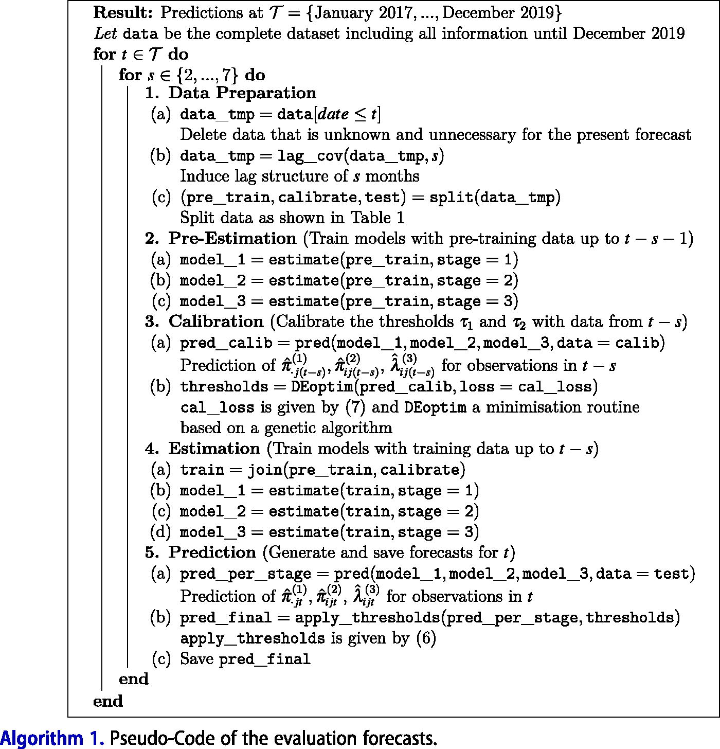In the same manner, we calculate expanding-window evaluation forecasts for January 2017 to December 2019 for all time-steps ($s=2,\dots ,7$) to measure the out-of-sample performance of our model. This procedure adequately replicates the real forecasting situation (Richardson, van Florenstein Mulder, and Vehbi 2020). In accordance with the real forecasts in (1), the prediction task of the evaluation is thus given by: (8) $$\text{log}\hspace{0.17em}(y_{\mathit{ijt}}+1)-\hspace{0.17em}\text{log}\hspace{0.17em}(y_{\mathit{ijt}-s}+1) \forall s=2,\dots ,7,i=1,\dots ,n_j,j=1,\dots ,n\text{and}t\in {\mathcal{T}}_{\mathit{Evaluation}},$$(8) where ${\mathcal{T}}_{Evaluation}=\{\mathrm{J}\mathrm{a}\mathrm{n}\mathrm{u}\mathrm{a}\mathrm{r}\mathrm{y}\mathrm{ }2017,\dots ,\mathrm{D}\mathrm{e}\mathrm{c}\mathrm{e}\mathrm{m}\mathrm{b}\mathrm{e}\mathrm{r}\mathrm{ }2020\}$ and given data until $t-s.$ The entire procedure for the latter type of prediction is summarized in Algorithm 1.⁶

For predicting the fatalities at time point $t$ and time-step $s,$ we use data until $t-s$ which we split into pre-training and calibration dataset according to Table 1 (sub-task 1). We start by estimating the model with the data from the pre-training data (sub-task 2). Consecutively, we optimize (7) given the calibration data (sub-task 3) and re-estimate the model on the training data (sub-task 4). Finally, we transform the forecasted fatalities at $t$ by applying (8) to ${\mathrm{\Delta }}_{ijt}^s$ and save the results (sub-task 5).

Application

We next employ the hierarchical hurdle regression model formulated above to forecast monthly changes in the intensity of fighting across the African continent. In particular, we focus on governmental arms imports and, on the PG level, their interaction with a location’s distance from the capital as theoretically critical covariates. We first discuss the construction of these and other covariates. Consecutively, we present out-of-sample evaluations of our proposed model as well as forecasts for October 2020 until March 2021.

Description of Covariates

The covariates, denoted by $x_{\cdot jt-s}^{(1)},x_{ijt-s}^{(2)}$ and $x_{ijt-s}^{(3)},$ can be specified for each stage individually. As discussed above, each regression model we calculate has a specific delay between target and regressor $s\in \{2,\dots ,7\}.$ For clarity, we define all covariates here before applying these model-specific lags.

For our key independent variable, governmental imports of major conventional weapons, we use data from the SIPRI Arms Transfer Database (SIPRI 2020a), covering global arms transfers from 1950 to the present. We construct two yearly variables from this dataset as we distinguish between “short-term” and “long-term” imports of weapons. The former cover the weapon imports during the present and previous year, while the latter sums up the procurements between three and ten years before the present year. We denote the corresponding yearly covariates by $x_{\cdot jy}^{LT}$ and $x_{\cdot jy}^{ST}$ for country $j$ and year $y$ to define them as: $$\begin{array}{c}{x}_{·jy}^{ST}=\hspace{0.17em}\text{log}\hspace{0.17em}(x_{j,y}^{\text{MCW Import}}+x_{j,y-1}^{\text{MCW Import}})\\ x_{·jy}^{LT}=\hspace{0.17em}\text{log}\left(\sum _{\tilde{y}=y-10}^{y-2}{x}_{j,\tilde{y}}^{\text{MCW Import}}\right),\end{array}$$ where $x_{j,y}^{\mathrm{M}\mathrm{C}\mathrm{W}\mathrm{ }\mathrm{I}\mathrm{m}\mathrm{p}\mathrm{o}\mathrm{r}\mathrm{t}}$ is given by the yearly import of major conventional weapons measured in TIVs (SIPRI 2020b). The temporal scale of the resultant covariates is then transformed from yearly to monthly by setting $x_{\cdot jt}^{ST}=x_{\cdot jy}^{ST}$ and $x_{\cdot jt}^{LT}=x_{\cdot jy}^{LT}$ for all months $t$ within year $y.$ In other words, short-term imports of MCW reflect the total strategic value of the weapons procured from abroad in the two years preceding an observation while long-term imports indicate the aggregate value of arms obtained in the eight years before that. As discussed above, we include these variables in all three stages of the model, but in stages 2 and 3 interact them with the location’s distance to the capital (Weidmann, Kuse, and Gleditsch 2010), which accordingly also enters stages 2 and 3 as a covariate. To capture the belligerents’ (potential) structural military power (Mehrl and Thurner 2020), we further include governmental military expenditures in all three stages (SIPRI 2019).

Additionally, our model contains three further groups of selected covariates. First, we account for spatial dynamics in our data by including a country-specific Gaussian random effect in the first stage as well as a smooth spatial effect of a location’s average longitude and latitude in all three stages. Second, we include a smooth time trend, dummy variables for month effects, the time since the last fatality as well as the total number of fatalities in the previous month resulting from organized violence to take temporal dynamics into account. Third, we incorporate a small number of covariates that have been shown to be key structural predictors of armed conflict onset and intensity (see Hegre et al. 2013, 2019). In Appendix A, a complete list of all included covariates is given with the respective data sources and transformations.

Results

Out-of-sample evaluation

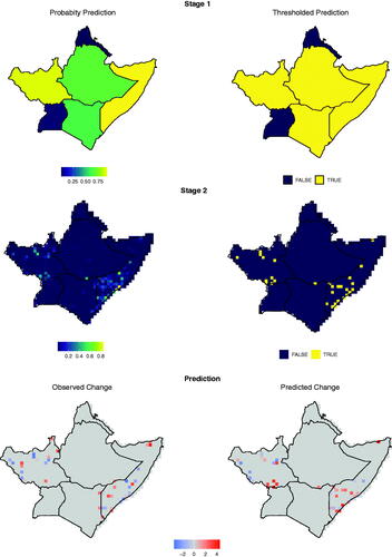
All three steps needed to obtain predictions for the number of state-based casualties in June 2018 with data until April 2018 ($s=2$) are illustrated in Figure 1 for a sub-sample of five countries in North-Eastern Africa (Eritrea, Ethiopia, Uganda, Somalia, Kenya, South Sudan). The first row depicts the predicted probability of country fighting incidence as well as whether the model expects violence to occur after applying the calibrated threshold. The second row presents these quantities for the cell level and shows that in this example, the optimized threshold probabilities at which the model expects fighting to take place differ from 0.5 (${\tau }_1=0.563,{\tau }_2=0.263$). In the third row, the final out-of-sample predicted fatalities in June 2018 are transformed to changes in conflict intensity. Here, we show the predictions on the right and the observed changes on the left side. A comparison of these two final maps suggests that our model is generally successful in identifying which countries will experience armed conflict as well as in predicting where those fatalities will occur. Notably, the model correctly identifies Eritrea and Uganda as not experiencing conflict in this month. On the sub-national scale, we predict both the location and the direction of, for instance, changes in the intensity of fighting in western South Sudan and southern Somalia rather well. At the same time, the maps demonstrate that our model was unable to forecast what seems like relatively isolated flare-ups of violence in, e.g. eastern Kenya.

Figure 1. Observed and predicted changes in fatalities ${\Delta }_{\mathit{ijt}}^s$ with s = 2 in June 2018 in a sub-sample of countries. The predictions are separated along Stage 1 (first row), Stage 2 (second row), and final predicted change to April 2018 (third row).

To evaluate the model in a more principled manner, we compare the out-of-sample performance of 1) the fully specified hierarchical hurdle regression model, 2) the same model without MCW imports and military capacities, and 3) the PGM benchmark model based on a random forest introduced by Hegre, Vesco, and Colaresi (2022) and Vesco et al. (2022). Let ${\widehat{y}}_{ts}$ be the stacked vector of all predictions at time point $t$ with data until $t-s,$ while the stacked predicted changes from (8) are denoted as $\mathrm{\Delta }{\widehat{y}}_{ts}$ and the matching observed values are $y_t$ and $\mathrm{\Delta }{y}_{ts}.$ Under this notation, the MSE and TADDA scores for $s=2,\dots ,7$ are given by: $$\begin{array}{l}MS{E}_s=\frac{1}{\text{\#}{\mathcal{T}}_{\mathit{Evaluation}}}\sum _{t\in {\mathcal{T}}_{\mathit{Evaluation}}}\frac{1}{\text{\#}{y}_t}{({\widehat{y}}_{ts}-y_t)}^2\\ T\mathit{ADD}{A}_s^{ϵ}=\frac{1}{\text{\#}{\mathcal{T}}_{\mathit{Evaluation}}}\\ \sum _{t\in {\mathcal{T}}_{\mathit{Evaluation}}}\frac{|\Delta y_{ts}-\Delta {\widehat{y}}_{ts}|+|\Delta {\widehat{y}}_{ts}|\mathbb{I}(\Delta {\widehat{y}}_{ts}^{(\pm )}\ne \Delta y_{ts}^{(\pm )})\mathbb{I}(|\Delta {\widehat{y}}_{ts}-\Delta y_{ts}|>ϵ)}{\text{\#}\Delta y_{ts}},\end{array}$$ where $\mathbb{I}(\cdot )$ is the indicator function, $y^{(\pm )}$ denotes the sign of all values in vector $y$ and $\mathrm{\#}y$ the dimension of $y,$ i.e., $\mathrm{\#}y=n$ for $y\in {\mathbb{R}}^n.$ Finally, $\epsilon$ is a value set at 0.048 to roughly correspond to a change of $5\mathrm{\%}$ in state-based fatalities. The resulting values are presented in Table 2. Overall, the MSE and TADDA scores are consistently higher for the benchmark model than for both hierarchical hurdle models. This indicates that accounting for the hierarchical structure of and excess zeroes within our data improves the ability to forecast conflict escalation and de-escalation. Simultaneously, these results suggest that weapons transfers and capabilities are key covariates when predicting the dynamics of state-based fighting. The out-of-sample validation hence provides clear support for our proposed model in terms of utilized model class and model specification.

Table 2. Out-of-sample MSE and TADDA scores from the hierarchical hurdle model with and without the MCW-related covariates as well as the benchmark model.

	MSE			TADDA
S	MCW	No MCW	Benchmark	MCW	No MCW	Benchmark
2	0.033	0.034	0.045	0.016	0.016	0.151
3	0.035	0.037	0.046	0.017	0.017	0.138
4	0.037	0.040	0.050	0.018	0.017	0.140
5	0.038	0.042	0.048	0.018	0.018	0.151
6	0.036	0.043	0.050	0.018	0.018	0.142
7	0.037	0.048	0.052	0.017	0.020	0.151

Forecasts

As already explained, we can exploit the proposed model to make monthly predictions up to March 2021. Figure 2 graphically presents the starting and end points of these forecasts. Similar to Figure 1, changes in conflict intensity are predicted to geographically cluster in a few regions which are often more distant to the corresponding country’s capital. One of these regions is the border area between Cameroon, Chad, Niger, and Nigeria, where Boko Haram has been particularly active. There, our model predicts violence to both de-escalate and escalate within the forecasting period. For October 2020, the forecast indicates that violence will decrease in most Nigerian locations but increase in PGs very close to Nigeria’s borders with Cameroon and Niger. In contrast, it expects violence to increase almost across the board in March 2021 as many locations both within Nigeria and bordering Cameroon and Niger are predicted to experience a rise in casualty numbers. The forecast concurrently expects Chad to remain unaffected by these changes in violence.

Figure 2. Forecasted log changes ${\Delta }_{\mathit{ijt}}^s$ in fatalities to October 2020 (s = 2) and March 2021 (s = 7), focused on the border region between Nigeria, Niger, Cameroon, and Chad.

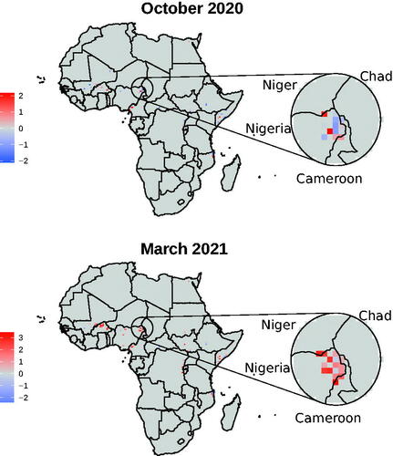
While less publicized than the Boko Haram case, Mozambique has also experienced the rise of a violent Islamist insurgency since its first attacks in 2017 (Morier-Genoud 2020). These insurgents have claimed numerous attacks in the country’s northeastern Cabo Delgado province and our model also predicts casualty numbers to shift in this region.⁷ It expects violence to move southwards along the coast as it predicts casualties to decrease in some of the northernmost areas of the province but to increase closer to its administrative center Pemba. Violence is thus expected to spread further within Cabo Delgado, reaching areas where the terrorist organization has previously shown little activity, but not across the border into Tanzania.

Finally, we present a subset of the linear estimates underlying the October 2020 forecasts in Table 3 (hence $s=2$) to examine to what extent weapons imports drive these predicted changes in violence. These results support our general expectation that arms imports fuel conflict. As suggested, at least long-term arms imports increase local conflict intensity, but this relationship becomes weaker for locations farther away from the capital. This conclusion is displayed in the negatively signed and statistically significant interaction terms in stage three. While there is little evidence that recent imports of MCW affect fighting at the PG-level, the estimates of stage 1, in contrast, allow drawing the inference that such transfers can trigger the country-level occurrence of fighting while longer-term imports are associated with a lower probability of lethal violence.

Table 3. The subset of the parametric estimates regarding the governmental procurement of weapons with s = 2 and training data from January 1990 to August 2020.

	Covariate	Estimate	Std. error	t-Value	p-Value
Stage 1	Military expenditure	0.0624	0.0511	1.2212	0.222
	Long-term import of MCW	−0.091	0.0453	−2.0075	0.0447
	Short-term import of MCW	0.1105	0.0286	3.8669	0.0001
Stage 2	Military expenditure	0.0917	0.0173	5.3150	<0.0001
	Distance to capital (CD)	0.0001	0.0001	1.2355	0.2167
	Long-term import of MCW (LT)	−0.0288	0.0229	−1.2530	0.2102
	Short-term import of MCW (ST)	−0.0642	0.0179	−3.5951	0.0003
	LT × CD	−0.0002	0.0000	−9.5278	<0.0001
	ST × CD	0.0000	0.0000	1.4594	0.1445
Stage 3	Military expenditure	0.1870	0.0438	4.2726	<0.0001
	Distance to capital (CD)	0.0020	0.0002	11.2856	<0.0001
	Long-term import of MCW (LT)	0.6842	0.0519	13.1847	<0.0001
	Short-term import of MCW (ST)	−0.0142	0.0418	−0.3397	0.7341
	LT × CD	−0.0009	0.0001	−12.7753	<0.0001
	ST × CD	−0.0002	0.0001	−3.5264	0.0004

These results contribute to clarifying our understanding of the relationship between arms imports and conflict intensity. They show that MCW imports do not escalate fighting immediately and everywhere, but that this effect instead takes some time to appear as troops take delivery of and get trained on the new weapons and is strongest close to the national capital. This points to the importance of logistical and infrastructure factors in the deployment of MCW and emphasizes the interplay of geographical and military endowments in determining incumbents’ ability to project power and wage war.

Our model thus performs well in out-of-sample predictions and enables users to understand how specific covariates affect the forecasts. This can add nuance to existing research and lead to new policy implications. The long-term effect of arms imports on conflict intensity uncovered here suggests that arms export bans as a reaction to fighting are insufficient to stop conflict escalation. Even peace-time exports, meant to stabilize politically challenged governments, can lead to increased bloodshed at the core of the state when fighting erupts. These results once more point to a need for stricter arms export policies.

Conclusion

Predicting the escalation and de-escalation of armed conflict at fine-grained spatio-temporal levels is a crucial concern to researchers and policymakers alike. In this article, we develop and apply a hierarchical hurdle regression model that explicitly accounts for two key features of conflict event data, namely hierarchical structure and excess zeroes. Inspired by recent calls to develop theoretically motivated conflict forecasting models, we, in particular, emphasize the role of governmental weapons imports as a potential driver of both country- and local-level fighting. Out-of-sample evaluations attest that both of our methodological and substantive contributions increase the ability to predict conflict (de-)escalations. We employ our modeling approach to forecast changes in the log-transformed number of casualties for October 2020 to March 2021. Showcasing the interpretability of our model, we further examine to what extent arms imports trigger and fuel violence. As a result, we find evidence that such transfers impact the occurrence and intensification of fighting in nuanced, previously unobserved ways. Overall, our model hence not only provides practitioners and policymakers with forecasts on future conflict escalation but can furthermore inform them about the principal drivers of—and hence levers to address—this fighting.

More generally, the hierarchical hurdle approach presented here will also be of interest to conflict scholars and forecasters due to its adaptability. For instance, its hurdle regression step could easily be appended to the binary ensemble model proposed in Hegre et al. (2019) by merely adding a conditional truncated layer onto the predicted posterior probabilities. Similarly, the semi-parametric specification we utilized in all three stages can easily be exchanged for arbitrary machine learning techniques.

Finally, this research points to the added value of including theoretically grounded processual covariates such as arms imports when forecasting conflict. As such, future work on conflict forecasting should leverage increasingly available fine-grained event data on other theoretically relevant covariates such as crop production, weather events, or migration. Along these lines, future research may also consider the influence of resources such as foreign aid which, in contrast to weapons, do not allow incumbents to deter or defeat challengers, but instead to buy them off, thus potentially decreasing the risk of conflict onset and escalation (Findley 2018). To better account for the serial dependencies and resulting self-exciting behavior, another possible enhancement of the covariates would be to incorporate self-exciting terms in the flavor of Porter and White (2012). Further, armed conflict is not the only type of event which is essential to forecast and occurs within a hierarchical data structure and with a wealth of excess zeroes. Hence, it would be fruitful to apply and extend our model to study any hierarchically clustered count data. Examples of such data are manifold and include the occurrence and local intensification of different types of conflict (e.g., one-sided or non-state), protests or infectious disease outbreaks.

Disclosure statement

No potential conflict of interest was reported by the author(s).

Correction Statement

This article was originally published with errors, which have now been corrected in the online version. Please see Correction (http://dx.doi.org/10.1080/03050629.2022.2101217).

Additional information

Funding

The work has been partially supported by the German Federal Ministry of Education and Research (BMBF) under Grant No. 01IS18036A. The project was also supported by the German Peace Science Foundation under Grant FP 08/16-SP 08/12-2015: International Arms Trade and Intrastate Conflict. The authors of this work take full responsibilities for its content.

Notes

1 For more details, see https://www.sipri.org/databases/armstransfers/background/coverage.

2 To be precise, almost 70% of fighting casualties occur in only four countries, namely Eritrea, Ethiopia, Sudan, and Somalia.

3 As we do not use the standard 25 battle death threshold for armed conflict, the first two classification stages of our model should not be interpreted as identifying conflict and non-conflict units.

4 This result follows from the direct calculation of the marginal density of $Y_{ijt}$ and the application of the total law of probability.

5 For our application the definition of those sets of covariates ($x_{ijt-s}^{(k,L)},x_{ijt-s}^{(k,NL)}$ with $k=1,2,3$) as well as the specification of smooth components are given in Appendix A.

6 This approach is used as contemporaneous covariates to forecast a target value are usually not available. To clarify, data until a specific point in time $t$ describes observations where the target variable was measured at $t$ and the covariates at $t-s.$ As we provide expanding-window forecasts, we run through the inner loop of Algorithm 1 (sub-task 1 through 5) for the prediction of each month ($\mathcal{T}=\{\mathrm{J}\mathrm{a}\mathrm{n}\mathrm{u}\mathrm{a}\mathrm{r}\mathrm{y}\mathrm{ }2017,\dots ,\mathrm{D}\mathrm{e}\mathrm{c}\mathrm{e}\mathrm{m}\mathrm{b}\mathrm{e}\mathrm{r}\mathrm{ }2019\}$) and time-step ($s=\{2,\dots ,7\}$), where we set the periodization according to Table 1.

7 See Figure 7 in Appendix C.

References

- Bagozzi, B. E. 2015. “Forecasting Civil Conflict with Zero-Inflated Count Models.” Civil Wars 17 (1): 1–24. doi:10.1080/13698249.2015.1059564.
- Beger, A., C. L. Dorff, and M. D. Ward. 2016. “Irregular Leadership Changes in 2014: Forecasts Using Ensemble, Split-population Duration Models.” International Journal of Forecasting 32 (1): 98–111. doi:10.1016/j.ijforecast.2015.01.009.
- Blair, R. A., and N. Sambanis. 2020. “Forecasting Civil Wars: Theory and Structure in an Age of ‘Big Data‘ and Machine Learning.” Journal of Conflict Resolution 64 (10): 1885–915. doi:10.1177/0022002720918923.
- Boulding, K. E. 1962. Conflict and Defense: A General Theory. New York: Harper.
- Buhaug, H. 2010. “Dude, Where’s My Conflict? LSG, Relative Strength, and the Location of Civil War.” Conflict Management and Peace Science 27 (2): 107–28. doi:10.1177/0738894209343974.
- Caverley, J. D., and T. S. Sechser. 2017. “Military Technology and the Duration of Civil Conflict.” International Studies Quarterly 61 (3): 704–20. doi:10.1093/isq/sqx023.
- Cederman, L.-E., and N. B. Weidmann. 2017. “Predicting Armed Conflict: Time to Adjust Our Expectations?” Science 355 (6324): 474–76. doi:10.1126/science.aal4483.
- Chiba, D., and K. S. Gleditsch. 2017. “The Shape of Things to Come? Expanding the Inequality and Grievance Model for Civil War Forecasts with Event Data.” Journal of Peace Research 54 (2): 275–97. doi:10.1177/0022343316684192.
- Cragg, J. G. 1971. “Some Statistical Models for Limited Dependent Variables with Application to the Demand for Durable Goods.” Econometrica 39 (5): 829–44. doi:10.2307/1909582
- Das, S., and P. N. Suganthan. 2011. “Differential Evolution: A Survey of the State-of-the-art.” IEEE Transactions on Evolutionary Computation 15 (1): 4–31. doi:10.1109/TEVC.2010.2059031.
- Domingos, P. 1999. “MetaCost: A General Method for Making Classifiers Cost-Sensitive.” In Proceedings of the Fifth ACM SIGKDD International Conference on Knowledge Discovery and Data Mining, KDD ’99,155–64. San Diego: Association for Computing Machinery. doi:10.1145/312129.312220.
- Eilers, P. H., and B. D. Marx. 1996. “Flexible Smoothing with B-splines and Penalties.” Statistical Science 11 (2): 89–102. doi:10.1214/ss/1038425655.
- Findley, M. G. 2018. “Does Foreign Aid Build Peace?” Annual Review of Political Science 213:59–384. doi: 10.1146/annurev-polisci-041916-015516.
- Hegre, H., G. Østby, and C. Raleigh. 2009. “Poverty and Civil War Events: A Disaggregated Study of Liberia.” Journal of Conflict Resolution 53 (4): 598–623. doi:10.1177/0022002709336459.
- Hegre, H., J. Karlsen, H. M. Nygård, H. Strand, and H. Urdal. 2013. “Predicting Armed Conflict, 2010–2050.” International Studies Quarterly 57 (2): 250–70. doi:10.1111/isqu.12007.
- Hegre, H., M. Allansson, M. Basedau, M. Colaresi, M. Croicu, H. Fjelde, F. Hoyles, L. Hultman, S. Högbladh, R. Jansen, et al. 2019. “ViEWS: A Political Violence Early-warning System.” Journal of Peace Research 56 (2): 155–74. doi:10.1177/0022343319823860.
- Hegre, H., P. Vesco, and M. Colaresi. 2022. “Lessons from an Escalation Prediction Competition.” International Interactions 48 (4): 000–000.
- Hernández-Orallo, J., P. Flach, and C. Ferri. 2012. “A Unified View of Performance Metrics: Translating Threshold Choice into Expected Classification Loss.” Journal of Machine Learning Research 13 (91): 2813–69. http//:jmlr.org/papers/v13/hernandez-orallo12a.html.
- Magesan, A., and E. L. Swee. 2018. “Out of the Ashes, into the Fire: The Consequences of U.S. Weapons Sales for Political Violence.” European Economic Review 1071: 33–156. doi: 10.1016/j.euroecorev.2018.05.003.
- Mehrl, M., and P. W. Thurner. 2020. “Military Technology and Human Loss in Intrastate Conflict: The Conditional Impact of Arms Imports.” Journal of Conflict Resolution 64 (6): 1172–96. doi:10.1177/0022002719893446.
- Morier-Genoud, E. 2020. “The Jihadi Insurgency in Mozambique: Origins, Nature and Beginning.” Journal of Eastern African Studies 14 (3): 396–412. doi:10.1080/17531055.2020.1789271.
- Mullahy, J. 1986. “Specification and Testing of Some Modified Count Data Models.” Journal of Econometrics 33 (3): 341–65. doi:10.1016/0304-4076(86)90002-3.
- Nelder, J. A., and R. W. M. Wedderburn. 1972. “Generalized Linear Models.” Journal of the Royal Statistical Society: Series A (General) 135 (3): 370–84. doi:10.2307/2344614.
- Pamp, O., L. Rudolph, P. W. Thurner, A. Mehltretter, and S. Primus. 2018. “The Buildup of Coercive Capacities: Arms Imports and the Outbreak of Violent Intrastate Conflicts.” Journal of Peace Research 55 (4): 430–44. doi:10.1177/0022343317740417.
- Pettersson, T., and M. Öberg. 2020. “Organized Violence, 1989–2019.” Journal of Peace Research 57 (4): 597–613. doi:10.1177/0022343320934986.
- Porter, M. D., and G. White. 2012. “Self-exciting Hurdle Models for Terrorist Activity.” Annals of Applied Statistics 6 (1): 106–24. doi:10.1214/11-AOAS513.
- Richardson, A., T. van Florenstein Mulder, and T. Vehbi. 2020. “Nowcasting GDP Using Machine-learning Algorithms: A Real-time Assessment.” International Journal of Forecasting 37(2): 941–48. doi:10.1016/j.ijforecast.2020.10.005.
- Ruppert, D., M. Wand, and R. J. Carroll. 2003. Semiparametric Regression. Cambridge: Cambridge University Press.
- Ruppert, D., M. Wand, and R. J. Carroll. 2009. “Semiparametric Regression during 2003–2007.” Electronic Journal of Statistics 3 (3): 1193–256. doi:10.1214/09-EJS525.
- Schneider, G., M. Bussmann, and C. Ruhe. 2012. “The Dynamics of Mass Killings: Testing Time-Series Models of One-Sided Violence in the Bosnian Civil War.” International Interactions 38 (4): 443–61. doi:10.1080/03050629.2012.697048.
- Sheng, V. S., and C. X. Ling. 2006. “Thresholding for Making Classifiers Cost-Sensitive.” In Proceedings of the 21st National Conference on Artificial Intelligence - Volume 1, AAAI’06, 476–81. Boston, MA: AAAI Press.
- SIPRI. 2019. Military Expenditure Database. Accessed September 30, 2019. https://www.sipri.org/databases/milex.
- SIPRI. 2020a. Arms Transfers Database. Accessed March 9, 2020. https://www.sipri.org/databases/armstransfers.
- SIPRI. 2020b. Arms Transfers Database: Sources and methods. Accessed March 9, 2020. https://www.sipri.org/databases/armstransfers/sources-and-methods.
- Tollefsen, A. F., and H. Buhaug. 2015. “Insurgency and Inaccessibility.” International Studies Review 17 (1): 6–25. doi:10.1111/misr.12202.
- Tollefsen, A. F., H. Strand, and H. Buhaug. 2012. “PRIO-GRID: A Unified Spatial Data Structure.” Journal of Peace Research 49 (2): 363–74. doi:10.1177/0022343311431287.
- Vesco, Paola, Håvard Hegre, Michael Colaresi, Remco Bastiaan Jansen, Adeline Lo, Gregor Reisch, and Nils B. Weidmann. 2022. “United They Stand: Findings from an Escalation Prediction Competition.” International Interactions 48 (4): 000–000. 10.1080/03050629.2022.2029856.
- Ward, M. D., N. W. Metternich, C. L. Dorff, M. Gallop, F. M. Hollenbach, A. Schultz, and S. Weschle. 2013. “Learning from the past and Stepping into the Future: Toward a New Generation of Conflict Prediction.” International Studies Review 15 (4): 473–90. doi:10.1111/misr.12072.
- Weidmann, N. B., D. Kuse, and K. S. Gleditsch. 2010. “The Geography of the International System: The CShapes Dataset.” International Interactions 36 (1): 86–106. doi:10.1080/03050620903554614.
- Wood, S. N. 2017. Generalized Additive Models: An Introduction with R. Boca Raton: CRC press.
- Wood, S. N. 2020. “Inference and Computation with Generalized Additive Models and Their Extensions.” Test 29:307–39. doi:10.1007/s11749-020-00711-5.