Predicting (de-)escalation of sub-national violence using gradient boosting: Does it work?

Abstract

This article presents a prediction model of (de-)escalation of sub-national violence using gradient boosting. The prediction model builds on updated data from the PRIO-GRID data aggregator, contributing to the ViEWS prediction competition by predicting changes in violence levels, operationalized using monthly fatalities at the 0.5 × 0.5-degree grid (pgm) level. Our model's predictive performance in terms of mean square error (MSE) is marginally worse than the ViEWS baseline model and inferior to most other submissions, including our own supervised random forest model. However, while we knew that the model was comparatively worse than our random forest model in terms of MSE, we propose the gradient boosting model because it performed better where it matters—in predicting when (de-)escalation happens. This choice means that we question the usefulness of using MSE for evaluating model performance and instead propose alternative performance measurements that are needed to understand the usefulness of predictive models. We argue that future endeavors using this outcome should measure their performance using the Concordance Correlation, which takes both the trueness and the precision elements of accuracy into account, and, unlike MSE, seems to be robust to the issues caused by zero inflation.

Este artículo presenta un modelo de predicción de la desescalada de la violencia subnacional mediante el uso de la potenciación del gradiente. El modelo de predicción se basa en los datos actualizados que provienen del agregador de datos de PRIO-GRID, contribuye al concurso de predicciones de ViEWS al predecir cambios en los niveles de violencia y es operacionalizado utilizando las muertes mensuales a nivel de cuadrícula de 0.5 × 0.5 grados (pgm). El rendimiento predictivo de nuestro modelo desde el punto de vista del error cuadrático medio (mean square error, MSE) es ligeramente peor que el modelo de referencia del sistema de alerta temprana sobre la violencia (Violence Early Warning System, ViEWS) e inferior en relación con la mayoría de las otras presentaciones, incluido nuestro modelo de bosque aleatorio y supervisado. No obstante, si bien sabíamos que el modelo era comparativamente peor que nuestro modelo de bosque aleatorio en relación con el MSE, proponemos el modelo de potenciación del gradiente porque funcionó mejor en el aspecto que importa: predecir cuándo ocurre la desescalada. Esta elección significa que cuestionamos la utilidad del uso del MSE para evaluar el rendimiento del modelo y, en cambio, proponemos mediciones de rendimiento alternativas que son necesarias para comprender la utilidad de los modelos predictivos. Sostenemos que, en los futuros proyectos en los que se utilice este resultado, se debería medir el rendimiento mediante la correlación de concordancia, la cual tiene en cuenta tanto los elementos de veracidad como los de precisión de la exactitud y, a diferencia del MSE, parece ser resistente a los problemas generados por la inflación cero.

Cet article présente un modèle de prédiction de la (dés)escalade de la violence infranationale utilisant un boosting de gradient. Ce modèle de prédiction repose sur des données à jour de l’agrégateur de données de la grille PRIO. Il contribue au concours de prédiction ViEWS (Violence early-warning system, système d’alerte précoce sur la violence) en prédisant les évolutions des niveaux de violence qui sont opérationnalisés sur la base du nombre mensuel de décès au niveau 0.5 × 0.5 degré de la grille (PGM). Les performances prédictives de notre modèle en termes d’erreur quadratique moyenne (EQM) sont légèrement moins bonnes que celles du modèle de référence ViEWS et inférieures à la plupart des autres modèles soumis, y compris à celles de notre propre modèle à forêt aléatoire supervisée. Cependant, bien que nous sachions que ce modèle à boosting de gradient était comparativement moins bon que notre modèle à forêt aléatoire en termes d’EQM, nous l’avons proposé car il était plus efficace dans le domaine qui compte : la prédiction du moment auquel une (dés)escalade interviendrait. Ce choix signifie que nous remettons en question l’utilité de l’utilisation de l’EQM pour évaluer les performances des modèles et nous proposons au lieu de cela des mesures de performances alternatives nécessaires pour comprendre l’utilité des modèles prédictifs. Nous soutenons que les futurs efforts utilisant ce résultat devraient plutôt mesurer leurs performances à l’aide de la Corrélation de concordance, qui prend à la fois en compte les éléments Exactitude et Précision et qui, contrairement à l’EQM, semble être robuste face aux problèmes causés par l’inflation zéro.

Keywords:

• Conflict
• statistical methodology
• Civil war
• GIS

View correction statement:

Correction

Introduction

This article presents a gradient boosting model using newly updated data from the PRIO-GRID v.3(alpha) data aggregator, contributing to the ViEWS prediction competition by predicting changes in violence levels, operationalized using monthly fatalities at the 0.5 × 0.5-degree grid (pgm) level (Hegre, Vesco, and Colaresi 2022). Our initial interest was in evaluating whether improved and new data-sources would yield improved predictions. However, the question quickly became how to measure predictive improvement for change in battle-related deaths (BRDs) at the pgm level. Three issues stand out as important: (a) how zero-inflation affects evaluation of predictive performance of accuracy, (b) the trade-offs of going from probabilistic prediction of events to point-prediction of change, and (c) how the outcome relates to the concept of (de-)escalation.

We submitted three different models to the competition. A gradient boosting model using the xgboost algorithm (Chen and Guestrin 2016) and a broad selection of input features, a random forest model with the same input features (Breiman 2001), and a null-model that simply predicts 0 in all cell-months. We show that the null-model is very good in terms of mean square error (MSE) due to zero-inflation in the pgm-scheme. The gradient boosting model was worse than the zero-model and the random forest model in terms of MSE. However, the gradient boosting model was more sensitive to signals of change than the random forest, and less dependent on its approximation towards the zero-model.

To think systematic around this, we provide a discussion around the two components of accuracy: trueness and precision, how we can measure these two components in terms of MSE/MAE and Pearson’s Correlation Coefficient, and how to weigh the two components using the Concordance Correlation Coefficient (Lin 1989) (${\rho }_c$). We argue that ${\rho }_c$ is superior compared to MSE/MAE at selecting the best model at the pgm level if we are more interested in anomaly detection than fitting the predictive mean (and that we should be in this case). We also discuss the extent to which TADDA is able to account for imprecisions at the pgm level and conclude that it reduces to MAE when outcomes are zero-inflated.

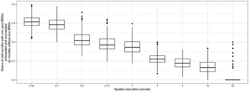
In addition, we discuss the trade-offs of moving from probabilistic event forecasting to point-forecasting of change in BRDs. As argued by Gneiting (2011), our baseline preference should be to prefer probabilistic forecasting over point-forecasting. From our perspective, the gains of moving to point-forecasting are that we can include, on the one hand, information about the intensity of violence and, on the other hand, trends in intensity of violence while it is ongoing (e.g., perhaps there is interesting information in the fact that intensity went down from 100 BRDs to 50). The intensity of violence could in principle be modelled through probabilistic forecasting, e.g., as a Poisson process or similar (returning the predicted distribution as your forecast). We are therefore left with the benefit that a measure of change appreciates trends in the data. We show, however, that this benefit is not applicable to at least 43% of cells with violence at the pgm level (see Figure 1). Since the benefits are small, we question the value of predicting change at high spatio-temporal resolutions.

Figure 1. Share of cell-months with recorded BRDs that did not observe violence the month before or after. Source: UCDP GED 20.1.

Finally, we pose the question if this dependent variable could/should be thought of as measuring conflict (de-)escalation. We argue that (de-)escalation should be thought of as a latent variable that needs to be modelled. The empirical question becomes whether there is sufficient information contained in event data at the pgm level to support a reliable model of (de-)escalation, and if so, whether the first-order difference in BRDs is the best operationalization of (de-)escalation. We argue that the pgm-level operationalization is not likely to capture what we commonly think of as (de-)escalation, and that more work needs to be put into developing measurements of (de-)escalation that can be better used to supervise models.

The Gradient Boosting Model

A core assumption in the ViEWS system is that what drives violence might vary across time and space (Hegre et al. 2019). To address this idea, the ViEWS system builds an ensemble of themed models (mostly trained through a random forest algorithm) that are given weights through a calibration process. Here, we test another approach, namely gradient boosting (Chen and Guestrin 2016). The gradient boosting algorithm commonly beats random forest on real-world tasks (Hastie, Tibshirani, and Friedman 2009; Chen and Guestrin 2016), which by itself is a sufficient motivation for exploring this algorithm.

Boosting algorithms build decision-trees in a serialized fashion, where observations poorly handled by the combined efforts of the previously fitted trees are weighted more heavily when fitting subsequent trees. The random forest algorithm, used in the current state-of-the-art in conflict early warning (Muchlinski et al. 2016; Hegre et al. 2019; Breiman 2001), is an ensemble method where bootstrapped samples are used to build de-correlated decision trees where each gets a vote in the final prediction (or in the case of regression: the average prediction across trees). The boosting algorithm we use, extreme gradient boosting (Chen and Guestrin 2016), also includes ideas from the random forest, such as taking bootstrapped samples when training each tree and sampling variables that can be evaluated at each node (i.e. de-correlating the trees).

In a random forest model, all performance improvements of the ensemble vis-à-vis an individual tree comes from variance reduction (Hastie, Tibshirani, and Friedman 2009, 601), the bias is the same in both (because each tree is identically distributed). In a boosting model, on the other hand, performance can also be improved through bias reduction. Another way to think of this is that in a boosting model, there is a place for specialized decision-trees. If we believe that the outcome we are trying to predict is a result of a set of (potentially highly varied) processes, i.e., one where the true process varies depending on where (and when) you look, then we could be missing out on performance gains by sticking to random forests. However, this potential gain could drown in other issues, such as boosting models being more prone to overfitting than the random forest.

As opposed to the random forest algorithm, a complication with gradient boosting is that we need to tune hyperparameters—a computationally intensive task. We use a set of parameters arrived at for another project with a slightly different dependent variable. The parameters were manually tuned using training data from 1998 to 2012 and testing from 2013 to 2015, with a binary dependent variable (whether a cell had observed organized armed conflict, based on the UCDP definition). We tuned using a combination of manual tuning and grid search, following guidelines by Jain (2016): Start with a high learning rate, an educated guess of the tree-specific parameters and no regularization, find a ballpark number of trees to train, tune the tree-specific parameters before regularization parameters, and only then lower learning rate and fine-tune. Our experience was that performance could vary significantly depending on the choice of hyperparameters. Since we have not fine-tuned our model for this learning task, there are likely some gains to be made by tuning more. Our tuning parameters can be found in the Supplementary Materials.

Data

High-quality data is imperative to predict with high spatial and temporal fidelity escalation and de-escalation of conflict. PRIO-GRID, a data-aggregator and -framework, has been used by many conflict researchers over the last decade (Tollefsen, Strand, and Buhaug 2012), including in the ViEWS project (Hegre et al. 2019). The framework has been updated periodically, from the initial release in 2012 to the first update in 2016. The sub-national data we use here is taken from our current efforts at updating PRIO-GRID to version 3 (see https://github.com/prio-data/priogrid). There are three significant changes in version 3(alpha): PRIO-GRID is now an R-package, it can be built to any spatio-temporal resolution (e.g., quarterly 1 × 1 degree cells), and we have added and removed several data-sources.

The improvements in version 3 should improve our ability to do early-warning. Some of the most important changes to the data, we believe, are the addition of the Subnational Human Development indicators (Smits and Permanyer 2019) and swapping out GlobCover2008 land cover data with FAO-GLCshare. Research has found that land cover datasets do not always agree on classifications, and GLCshare is found to be among the best performing datasets (Pérez-Hoyos et al. 2017). Both our random forest and our gradient boosting model are using 48 predictors in all, where 12 are country-level predictors, and 36 are sub-national level predictors. Table 1 provides an overview of the predictors.

Table 1. Predictors. Sub-national level variables were calculated using the PRIO-GRID v.3(alpha) framework.

Variable	Description	Source
ged_best_(sb|ns|os)_sum12	UCDP GED Candidate Dataset sum of state-based, non-state, and onesided violence (respectively) over a moving 12-month window	(Hegre et al. 2020)
ged_best_(sb|ns|os)_sum12grwtr6	6-month moving average growth of each of ged_best_(sb|ns|os)_sum12	(Hegre et al. 2020)
quad(1–4) and protest	Count of ICEWS events at the country-month level, separate variables for (verbal cooperation, material cooperation, verbal conflict, material conflict, protest)	(Boschee et al. 2018)
homicide	Global Burden of Disease 2017 country-year homicide rates	(Global Burden of disease Collaborative Network 2018)
v2x_clphy	Varieties of Democracy v.10 physical integrity index	(Coppedge et al. 2020)
v2x_libdem	Varieties of Democracy v.10 liberal democracy index	(Coppedge et al. 2020)
eld2m	REIGN 2-month half-life time until election day at country-month level	(Bell 2016)
esch	SHDI expected years of schooling at entrance age	(Smits and Permanyer 2019)
msch	SHDI mean years of schooling of adults aged 25+	(Smits and Permanyer 2019)
gnic	SHDI gross national income per capita	(Smits and Permanyer 2019)
lifexp	SHDI life expectancy at birth	(Smits and Permanyer 2019)
glcs_(landcovertype)	GLC-SHARE share of land covered with artificial surfaces, cropland, grassland, shrubs, mangroves, trees, freshwater, and snow, respectively	(Latham et al. 2014)
capdist	cShapes v.0.6 distance to capital	(Weidmann, Kuse, and Gleditsch 2010)
bdist3	cShapes v.0.6 distance to nearest internal border	(Weidmann, Kuse, and Gleditsch 2010)
riverdist	GSHHG v.2.3.7 distance to nearest major river or lake	(Wessel and Smith 1996)
coastdist	GSHHG v.2.3.7 distance to nearest coast	(Wessel and Smith 1996)
ruggedness	Terrain ruggedness	(Shaver, Carter, and Shawa 2019)
temp	CRU TS4.04 monthly gridded temperature	(Harris et al. 2020)
pre	CRU TS4.04 monthly gridded precipitation	(Harris et al. 2020)
spei(1,3,6,12,24)	Standardized Precipitation- and Evapotranspiration Index (1,3,6,12,24)-month intervals respectively using CRU TS4.04	(Harris et al. 2020)
waterrisk	WRI Aqueduct 3.0 Composite Water Risk Index (static)	(Hofste et al. 2019)
pop_gpw_sum	GPW 4.0 gridded yearly population (interpolated from 5-year data)	(CIESIN 2018)
eth_(promoted|demoted|excluded)	ETH EPR count of groups (promoted|demoted|excluded) at country-month	(Vogt et al. 2015)
epr_(promoted|demoted|excluded)	GeoEPR count of groups (promoted|demoted|excluded) at grid-month	(Vogt et al. 2015)
epr_regional	GeoEPR presence of regional groups (static)	(Vogt et al. 2015)

All variables were lagged 6 months.

Our dependent variable is growth in battle-related deaths (state-based) (using the log method, as indicated in the competition guidelines) [depvar] (Hegre, Vesco, and Colaresi 2022, A-2). Following the ViEWS competition guidelines, we supply predictions for January 2014 until July 2016, January 2017 until July 2019, and October 2020 until March 2021. To reduce the amount of computation and simulate the anticipated time required to collect all data, we have lagged all predictors for 6 months. We only estimate the model anew each 6 months, so predictions for June 2016 are based on the same statistical model as for January 2016 until May 2016. Lastly, we included a lag of 2 months between training and testing to accommodate the anticipated time to estimate the model. For the historical predictions, s2 are January and July, while s7 are June and December. For the actual forecast, we estimated the model once, with outcome data from August 2020 and predictors from February 2020 (i.e., lagged 6 months). Using the ViEWS lingo, Oct 2020 is, therefore, s2, while March 2021 is s7. We deem our setup as feasible to deploy in real-time, and we have production-level code to build the complete dataset and run estimations.

On Evaluating Accuracy

According to the ISO 5725 standard (ISO 1994), accuracy can be broken down into trueness (closeness of the mean of a set of values to the true) and precision (closeness of agreement among this set). It is quite common, however, to use accuracy in place for trueness, even in highly specialized analytical settings (Menditto, Patriarca, and Magnusson 2007). One reason for this could be that optimizing for trueness can yield improvements also for precision. This is not necessarily the case, however (Pandit and Schuller 2020).

One rule of thumb is that we should not only be optimizing for trueness when the predictive mean is a poor representation of the data (Czado, Gneiting, and Held 2009), for instance, if the true distribution is zero-inflated and overdispersed. When building point-forecasts, however, we are not evaluating the whole predictive distribution. As Gneiting (2011) points out, unless the scoring function is specified ex ante, evaluating point-forecasts can quickly deteriorate into data-mining of the predictive distribution. At the same time, if we are using point-forecasts, then the scoring function specified ex ante should be properly motivated.

The outcome used here has a median of 0, mean of 0.000027, minimum value –10.78 and maximum value 10.31 (using data between 1995 and 2019). 99.56% of all observations are zeroes. We contend that we should not only be interested in trueness (i.e., getting the predictive mean right). Rather, we are interested in models that can detect anomalies from zero. Since the mean square error (MSE) is a measurement of trueness (e.g., Czado, Gneiting, and Held 2009, 1257f), using MSE as the point-forecast scoring function is poorly motivated.

As a case in point, the null model (MSE = 0.032) beats the ViEWS benchmark model (MSE = 0.047) by some margin. If the forecast task were oblivious to precision, and only cared about the long-run expected "gains" by betting on one model, it would be reasonable to scrap the ViEWS model. However, that is not why we are interested in building these models.

What are our alternatives? One is to build models that return predictive distributions and evaluate these using scoring functions that consider the whole distribution (Czado, Gneiting, and Held 2009). Another is to combine the evaluation of trueness with the evaluation of precision. In the following, we consider the latter alternative. $$\rho =\mathrm{ }\frac{\mathit{cov}(X,\mathrm{ }Y)}{{\sigma }_X{\sigma }_Y}$$

We start our consideration with the Pearson correlation coefficient (ρ). ρ is a measurement of precision. More precisely, it measures the extent of linear relationship between two variables. However, it completely ignores the trueness. Lin (1989) effectively shows this using the idea that accuracy (i.e., trueness + precision) could be thought of as the degree to which the true values and the predicted values fall on a 45° line through the origin when plotted in a scatter-plot. ρ fails to capture location shifts (i.e., where Y is different from X by a constant A) and scale shifts (i.e., where Y is different from X by a multiplicative factor α) or a combination of these. Lin (1989) suggests to augment ρ with a bias correction factor C where, $$C={\left[\frac{\nu +\frac{1}{\nu }+u^2}{2}\right]}^{-1}$$ $$\nu =\frac{{\sigma }_1}{{\sigma }_2}=\mathit{scale}\mathrm{ }\mathit{shif}\mathrm{t}$$ $$u=\frac{u_1-u_2}{\sqrt{{\sigma }_1{\sigma }_2}}=\mathit{location}\mathrm{ }\mathit{shift}\mathrm{ }\mathit{relative}\mathrm{ }to\mathrm{ }\mathit{the}\mathrm{ }\mathit{scale}$$ $${\rho }_c=\mathrm{ }\rho C=\mathrm{ }\frac{2{\sigma }_{12}}{{\sigma }_1^2+\mathrm{ }{\sigma }_2^2+{\left(u_1-u_2\right)}^2}$$

Unlike ρ, ${\rho }_c$ (the Concordance Correlation Coefficient) does evaluate the extent to which observations fall on the 45° line through the origin, and therefore the accuracy. ${\rho }_c$ falls within the [–1, 1] range, where 0 signals no agreement, 1 signifies perfect agreement, and –1 signifies perfect disagreement. Correlations close to zero should be regarded as very poor and unreliable for use in forecasting.

${\rho }_c$ is a perfect measurement of accuracy when we believe that our measurement of the outcome is exactly what we want to match, such as when the outcome is without measurement errors or in reproducibility studies. Conflict is not measured without errors, and the forecasting skill of a model will not be improved by fitting better to noise, meaning that higher ${\rho }_c$ does not necessary translate into improved forecasting skill. When evaluating ${\rho }_c$ (and ρ), we should have this in mind. While MSE is arguably more robust against such noise, we worry that using MSE for our outcome at the pgm level is throwing the baby out with the bathwater—that it is unable to differentiate models that can predict spikes from those that are not.

What we have considered here is the accuracy between two continuous variables. As exemplified by the ViEWS competition scoring guidelines, other issues regarding the measurement of accuracy can arise. The pseudo-Earth Mover Divergence (pEMDiv) (Greene et al. 2019) considers the idea that predicting escalation in areas close to where escalation actually happened is more correct than predicting it farther away. The Targeted Absolute Distance with Direcation Augmentation (TADDA) adds a penalty to predicting escalation when de-escalation happened, and vice-versa, as well as a penalty to predicting zero (de-)escalation when (de-)escalation happened, with the aim to select for models that are particularly good at separating escalation, de-escalation, and no-change. $$\mathit{TADDA}=\mathrm{ }\frac{\sum \left|Y-\mathrm{ }\widehat{Y}\right|+\widehat{\left|Y\right|}I[Y^{\pm }\ne \widehat{Y^{\pm }}]I\left[\right|Y-\widehat{Y}|>\epsilon ]}{N}$$

While TADDA does include a penalty for models that predict zeroes when the truth is non-zero (with threshold ε), there is a worry still that trueness overwhelms precision. The reason is that the penalty is additive and proportional to the size of cell-months with observed BRDs. Consider and compare with ${\rho }_c,$ where trueness and precision are weighed equally and multiplicatively. Near zero precision and high trueness yields near zero score. With TADDA, the same scenario would yield almost the same score as for MSE when the share of zero observations become large.

Evaluation of Model Performance

Figure 2 shows the model rank per metric for ten different models and five metrics. The models we submitted to the competition was the Null model and the two main (6 m lag) models (Random Forest and xgboost). To further explore the metrics, we have added models with more conflict history (using 1 m lag of predictors and adding counts of BRDs split on conflict type for the month before). We also test attenuating the xgboost model estimates toward zero by multiplying all predictions with .25. Figure 3 shows all point estimates for these models [triangle] as well as for additional models using PRIO-GRID year (pgy) [square] and country-month resolution models (cm) [circle], both using absolute estimate and truth [left column] and the normal approach [right column].

Figure 2. Performance evaluation based on model rank per metric. Colors in online version.

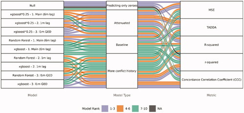
Figure 3. Performance metrics for predictions between 2014 and 2019. CCC (${\rho }_c$) is bound between [–1,1], r-squared is bound between [0,1], R-squared is bound between [–∞,1], while MSE and TADDA are bound between [0, ∞]. Higher is better for CCC, r-squared and R-squared, while lower is better for MSE and TADDA. Colors in online version.

The metrics we calculate are the mean square error (MSE), TADDA, the coefficients of determination (both r-squared and R-squared), and the concordance correlation coefficient (${\rho }_c$). R² can be calculated either as ρ² (r-squared), or as 1- MSE/Var(Y) (R-squared). In the latter definition, the relative ranking of models is identical with MSE, because Var(Y) does not change across models. R-squared is useful as a standardization of MSE that can be compared across samples, e.g., for future reference, while r-squared is a useful reference point to see how important the bias factor is in ${\rho }_c.$

What Figure 2 tells us is that MSE, TADDA, and R-squared tend to favor the zero model, attenuated models, or models without more conflict history included. r-squared and the CCC, on the other hand, favors models with conflict history. We see the same patterns for pgy-level models, but with a more mixed picture for cm-level models (where all metrics favor models with more conflict history).

TADDA and MSE yield very similar results. The main difference is that TADDA is based on mean absolute errors, which penalize outliers less than MSE. The result is that TADDA has an even stronger affinity towards the Null model. The bias-correction in TADDA can only be observed at the 3rd or 4th decimal (for values around .1) when comparing TADDA and MAE. We think the reason is that TADDA reduces to MAE as zero-inflation goes to 1 due to N in the denominator and the size of the numerator being dependent on the size of non-zero observations.

Since TADDA is not doing work to distinguish models that separate positive and negative values from those that struggle with this, we suggest comparing model performance between the left and right column in Figure 3. Note that we cannot directly compare MSE and TADDA, as these values are absolute and not relative. The differences in R-squared, r-squared and ${\rho }_c$ are clear for models without access to recent conflict history (e.g., ${\rho }_c$ goes from 0 to .16 in the xgboost model), but larger for xgboost than for random forest. The differences are smaller for models with access to recent conflict history, but with slight improvements when not having to separate positive and negative spikes (${\rho }_c$ is around .4, r-squared around .2, and R-squared around -.8 in both cases for xgboost). Looking at a few time-series for cells with violent events shows that adding 1-month lags enables the model to predict both (to some extent) positive spikes and (definitively) the subsequent negative spike (see Supplementary Materials for plots), while models without such variables are mostly non-responsive to the spikes.

If we want models that can fit to the observed spikes in the outcome (and not just have a well calibrated predicted mean), we found ${\rho }_c$ and r-squared to be more useful performance measurements than MSE, TADDA, and R-squared. r-squared and ${\rho }_c$ ranks models similarly at the pgm, pgy, and cm levels, but the bias adjustment in ${\rho }_c$ does come into play in certain cases. For instance, at the cm level, MSE and r-squared agrees that the Random Forest with 1-month lag GED counts is best, while ${\rho }_c$ scores the xgboost model with 1-month lag GED counts higher. Further research is needed to understand these trade-offs better. We observe that the choice of algorithms has relatively little to say, perhaps with a small advantage to xgboost over random forest (considering that we use the same hyperparameters for all our models).

An argument could be made that our output is noisy, and that the precision-based metrics are better at capturing noise, while trueness-based metrics are better at capturing the signal from the underlying data-generating process. This interpretation would lead us to think that adding 1-month lag of the dependent variable to models induce more noise than signal, since MSE increases when doing so. This might be true. However, from Czado, Gneiting, and Held (2009), we get that trueness-based metrics such as MSE is not suitable for capturing the signal when the data-generating process is not Gaussian, something which is highly likely in our case (the count data is zero-inflated and overdispersed). An alternative interpretation is therefore that the trueness-indicators are throwing the baby out with the bathwater, meaning that point-prediction evaluation of change in conflict intensity at the pgm level is unable to separate noise and signal.

If the latter interpretation is true, we have some alternatives: One alternative is to report the whole predictive distribution and evaluate that (and not only the predictive mean), as suggested in Czado, Gneiting, and Held (2009). A second alternative is to accept that we are not able to separate signal from noise at high spatio-temporal resolutions, rather use precision-based approaches to evaluate performance, and hope that it will translate into improved forecasting skill. A third alternative is to think more theoretically through what (de-)escalation means, and how we can reliably measure it.

Are we Measuring (de-)Escalation?

The Cambridge Dictionary defines escalation as "a situation in which something becomes greater or more serious." A conflict can become more serious in many ways. Bartusevičius and Gleditsch (2019) argue that conflicts can usefully be understood using a two-stage approach, where the relationship between two groups can escalate from peace into a contested incompatibility (conflict origination), and then into violence (conflict militarization). Conflicts can become more serious if they become more difficult to end. A classical case could be if another party enters the conflict, or if one party splits into more factions, making it more difficult to reach negotiated settlements (Walter 2009). Conflicts can also become more serious if the risk of future violence increases. The rationale for measuring the change in fatalities in an area over time is to capture this latter kind of escalation.

However, a change in fatalities in an area over a given time is not the same as (de-)escalation. It becomes clear at the limits, for instance if time is measured in seconds. The fact that one combatant died one second ago does not mean the conflict has de-escalated now. At the opposite scale of the spectrum, there is an ongoing debate in conflict research whether the total risk of (death from) conflict in the world has gone down (since WWII and further back) (Pinker 2011; Cunen, Hjort, and Nygård 2020). The variable of interest—(de-)escalation—is latent. Measuring change in BRDs (at the pgm level) is but one operationalization of that latent dimension, and it is possible to discuss the validity and reliability of such an operationalization (and perhaps it turns out to be a many-faceted concept with many valid operationalizations).

The fact that we are doing well using the pEMDiv (Vesco et al. 2022, Figure D-8) but poor in cell-month specific performance metrics could be attributed to potential noise in the operationalization of (de-)escalation, or that our input features are capturing broader structures while the pgm operationalization values models that capture micro-structures. For instance, consider a cell with high fatality events every other month. The pattern could have been produced by a conflict experiencing a rollercoaster pattern of (de-)escalation, or the conflict risk could have been always equally high—but with actualizations of this risk every other month. While a cell-month specific point-performance metric could easily conclude that a model capturing the risk is terrible, a probabilistic approach or the pEMDiv approach does alleviate the issue. It would be even better to align/define the outcome variable (used for model supervision) so that the models are properly trained, and input features have a chance to fit well to the signal. In our case, our input features are not well aligned to the outcome (and vice versa).

Figures 4 shows a concrete example from the data in the border areas between Nigeria/Chad/Cameroon (2C) and Mozambique/Tanzania (2D). We can see that "escalation" and "de-escalation" happens as subsequent pulses over several years (the black line is the actual outcome). A more useful measurement of escalation would have been to denote when the frequency/seriousness of events changed substantially, such as estimated through a change-point model, or through aggregations of events over longer time-periods. From visual inspection, in some of the cells, the event risk seems to be stable across the three-year period, while in others, there might be a few (de-)escalatory periods. The spatio-temporal resolution possible to achieve whilst still reliably measuring (de-)escalation could very well vary across time and space.

Figure 4. Zoom of the forecasts for Nigeria/Cameroon/Chad border (A + C) and Mozambique/Tanzania border (B + D). A + B shows the xgboost model's forecasts for October 2020 and the sum of battle-related deaths over the last year (since August 2020) in red. C + D shows the predictions (red, green, and blue line) plotted against the actual (black line) for the same cells as in A + B from January 2017 until December 2019. Colors in online version.

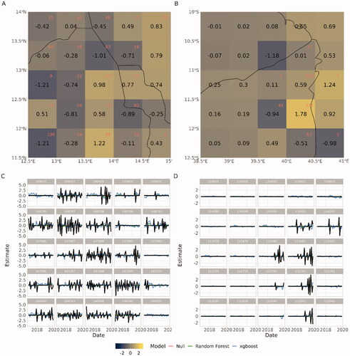
The negative pulses following positive pulses, seen in Figure 4, should be given some consideration when thinking about how to optimally define (de-)escalation. Figure 1 shows how often violence is observed in a cell-month without violence in the month before and after at varying spatial resolutions. For instance, for the pgm resolution (0.5), 43% of the cell-months that did observe violence did not observe any violence either before or after. For these observations, we have essentially transformed the information of BRDt0 into a tuple (BRDt0, -BRDt1). These tuples act more as noise than information if the goal is to fit input features to (de-)escalatory signals, and models using 1-month lag outcome data have an easy time fitting to this pulse. This capacity is not prediction of de-escalation at t + 1, but rather just the observation that violence on time t. In the Supplementary Materials, we show anecdotal evidence that it is this negative pulse we are mainly able to “predict” using 1 m lags of GED counts at the pgm level.

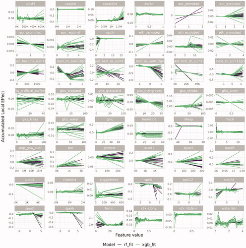
Figure 5 shows the accumulated local effects (Apley and Zhu 2019) for each variable in our main gradient boosting model (green lines) and main the random forest model (purple lines). The accumulated local effect makes arbitrary shifts between being positive and negative across the value range for a wide range of variables. In other words, the model has trouble separating the process determining positive values and the process determining negative values in the outcome. We believe that the way escalation and de-escalation is defined when using monthly changes in fatalities makes it very difficult for the algorithm to find any signal separating positive and negative values in the data using these predictors.

Figure 5. Accumulated local effects. Colors in online version.

Forecasts

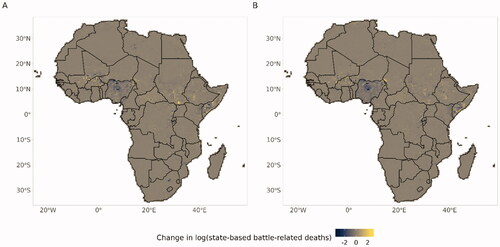
Based on our performance evaluation, we do not believe that the forecasts generated from our main model are able to separate escalatory and de-escalatory processes, nor that we are able to predict (de-)escalatory spikes very well (with a CCC of .16 at the highest). Furthermore, from our discussion on whether what we are measuring should be thought of as escalation, we want to highlight that different operationalizations of the dependent variable are likely to capture/value different aspects of conflict dynamics. Our model is able to roughly point to places and times where conflict history and structural conditions tell us that conflict risk is high (as measured by pEMDiv), but not skillfully predict the micro-dynamics of violence intensities. Despite these big caveats, and for the sake of transparency, we show our point forecasts in Figure 6.

Figure 6. The maps show the forecasts from the xgboost model for (A) October 2020 and (B) March 2021.

Acknowledgements

The authors would like to thank Michael Colaresi, Håvard Hegre, Paola Vesco, and two anonymous reviewers for great comments, discussions, and help.

Correction Statement

This article was originally published with errors, which have now been corrected in the online version. Please see Correction (http://dx.doi.org/10.1080/03050629.2022.2101217).

Additional information

Funding

This research has received financial support from the European Research Council through grant 648291 and from the European Union’s Horizon 2020 research and innovation program under grant agreement no. 769886.

References

- Apley, Daniel W., and Jingyu Zhu. 2020. “Visualizing the Effects of Predictor Variables in Black Box Supervised Learning Models.” Statistical Methodology, Series B 82 (4): 1059-1086. doi:10.1111/rssb.12377.
- Bartusevičius, Henrikas, and Kristian Skrede Gleditsch. 2019. “A Two-Stage Approach to Civil Conflict: Contested Incompatibilities and Armed Violence.” International Organization 73 (1): 225–248. doi:10.1017/S0020818318000425.
- Bell, Curtis, Besaw, Clayton., Frank, Matthew. 2021. “The Rulers, Elections, and Irregular Governance (REIGN) Dataset.” Broomfield, CO: One Earth Future. Accessed June 26, 2020. https://oefdatascience.github.io/REIGN.github.io/.
- Boschee, Elizabeth, Jennifer Lautenschlager, Sean O'Brien, Steve Shellman, and James Starz. 2018. “ICEWS Weekly Event Data.” Harvard Dataverse. Accessed November 15, 2021. doi:10.7910/DVN/QI2T9A.
- Breiman, Leo. 2001. “Random Forests.” Machine Learning 45 (1): 5–32. doi:10.1023/A:1010933404324.
- Chen, Tianqi, and Carlos Guestrin. 2016. “XGBoost: A Scalable Tree Boosting System.” In Proceedings of the 22nd ACM SIGKDD International Conference on Knowledge Discovery and Data Mining, edited by Balaji Krishnapuram, Mohak Shah, Alex Smola, Charu Aggarwal, Dou Shen, and Rajeev Rastogi, 785–94. New York: Association for Computing Machinery. Accessed November 10, 2021. doi:10.1145/2939672.2939785.
- CIESIN. 2018. Gridded Population of the World, Version 4 (GPWv4): Population Density, Revision 11.” Palisades, NY: NASA Socioeconomic Data and Applications Center (SEDAC). Accessed November 10, 2021. doi:10.7927/H49C6VHW.
- Coppedge, Michael, John Gerring, Carl Henrik Knutsen, Staffan I. Lindberg, and Jan Teorell, 2020. “V-Dem Country-Year Dataset V10.” University of Gothenburg: Varieties of Democracy (V-Dem) project.
- Cunen, Céline, Nils Lid Hjort, and Håvard Mokleiv Nygård. 2020. “Statistical Sightings of Better Angels: Analysing the Distribution of Battle-Deaths in Interstate Conflict over Time.” Journal of Peace Research 57 (2): 221–234. doi:10.1177/0022343319896843.
- Czado, Claudia, Tilmann Gneiting, and Leonhard Held. 2009. “Predictive Model Assessment for Count Data.” Biometrics 65 (4): 1254–1261. doi:10.1111/j.1541-0420.2009.01191.x.
- Global Burden of Disease Collaborative Network. 2018. Global Burden of Disease Study 2017 (GBD 2017) All-cause Mortality and Life Expectancy 1950–2017. Seattle: Institute for Health Metrics and Evaluation (IHME). Accessed January 14, 2020. http://ghdx.healthdata.org/record/ihme-data/gbd-2017-all-cause-mortality-and-life-expectancy-1950-2017
- Gneiting, Tilmann. 2011. “Making and Evaluating Point Forecasts.” Journal of the American Statistical Association 106 (494): 746–762. doi:10.1198/jasa.2011.r10138.
- Greene, Kevin, Håvard Hegre, Frederick Hoyles, and Michael Colaresi. 2019. “Move It or Lose It: Introducing Pseudo-Earth Mover Divergence as a Context-Sensitive Metric for Evaluating and Improving Forecasting and Prediction Systems.” Paper presented at Barcelona School of Economics Summer Forum 2019, Barcelona, Spain, June 19.
- Harris, Ian, Timothy J. Osborn, Phil Jones, and David Lister. 2020. “Version 4 of the CRU TS Monthly High-Resolution Gridded Multivariate Climate Dataset.” Scientific Data 7 (1): 1–18. doi:10.1038/s41597-020-0453-3.
- Hastie, Trevor, Robert Tibshirani, and J. H. Friedman. 2009. The Elements of Statistical Learning: Data Mining, Inference, and Prediction. 2nd ed. Springer Series in Statistics. New York: Springer.
- Hegre, Håvard, Marie Allansson, Matthias Basedau, Michael Colaresi, Mihai Croicu, Hanne Fjelde, Frederick Hoyles, et al. 2019. “ViEWS: A Political Violence Early-Warning System.” Journal of Peace Research 56 (2): 155–174. doi:10.1177/0022343319823860.
- Hegre, Håvard, Mihai Croicu, Kristine Eck, and Stina Högbladh. 2020. “Introducing the UCDP Candidate Events Dataset.” Research and Politics 7(3): 1–8.
- Hegre, Håvard, Paola Vesco, and Michael Colaresi. 2022. “Lessons from an Escalation Prediction Competition.” International Interactions 48 (4): 000-000.
- Hofste, Rutger Willem, Samantha Kuzma, Sara Walker, Edwin H. Sutanudjaja, Marc F.P. Bierkens, Marijn J.M. Kuijper, Marta Faneca Sanchez, Rens Van Beek, Yoshihide Wada, Sandra Galvis Rodrıǵuez, and Paul Reig. 2019. “Aqueduct 3.0: Updated Decision-Relevant Global Water Risk Indicators.” World Resources Institute. Accessed November 15, 2021. https://doi.org/10.46830/writn.18.00146
- ISO. 1994. ISO 5725-1: Accuracy (Trueness and Precision) of Measurement Methods and Results. ISO. 1994. Accessed March 4, 2021. https://www.iso.org/cms/render/live/en/sites/isoorg/contents/data/standard/01/18/11833.html
- Jain, Aarshay. 2016. “XGBoost Parameters | XGBoost Parameter Tuning.” Analytics Vidhya (blog), March 1, 2016. https://www.analyticsvidhya.com/blog/2016/03/complete-guide-parameter-tuning-xgboost-with-codes-python/.
- Latham, John, Renato Cumani, Ilaria Rosati, and Mario Bloise. 2014. Global Land Cover Share (GLC-SHARE) Database Beta-Release Version 1.0-2014. Rome: FAO.
- Lin, Lawrence I-Kuei. 1989. “A Concordance Correlation Coefficient to Evaluate Reproducibility.” Biometrics 45 (1): 255–268. doi:10.2307/2532051.
- Menditto, Antonio, Marina Patriarca, and Bertil Magnusson. 2007. “Understanding the Meaning of Accuracy, Trueness and Precision.” Accreditation and Quality Assurance 12 (1): 45–47. doi:10.1007/s00769-006-0191-z.
- Muchlinski, David, David Siroky, Jingrui He, and Matthew Kocher. 2016. “Comparing Random Forest with Logistic Regression for Predicting Class-Imbalanced Civil War Onset Data.” Political Analysis 24 (1): 87–103. doi:10.1093/pan/mpv024.
- Pandit, Vedhas, and Björn Schuller. 2020. “The Many-to-Many Mapping Between the Concordance Correlation Coefficient and the Mean Square Error.” ArXiv:1902.05180 [Cs, Math, Stat], July. http://arxiv.org/abs/1902.05180.
- Pérez-Hoyos, Ana, Felix Rembold, Hervé Kerdiles, and Javier Gallego. 2017. “Comparison of Global Land Cover Datasets for Cropland Monitoring.” Remote Sensing 9 (11): 1118. doi:10.3390/rs9111118.
- Pinker, Steven. 2011. The Better Angels of Our Nature: The Decline of Violence in History and Its Causes. London: Penguin UK.
- Shaver, Andrew, David B. Carter, and Tsering Wangyal Shawa. 2019. “Terrain Ruggedness and Land Cover: Improved Data for Most Research Designs.” Conflict Management and Peace Science 36 (2): 191–218. doi:10.1177/0738894216659843.
- Smits, Jeroen, and Iñaki Permanyer. 2019. “The Subnational Human Development Database.” Scientific Data 6 (1): 1–5. doi:10.1038/sdata.2019.38.
- Tollefsen, Andreas Forø, Håvard Strand, and Halvard Buhaug. 2012. “PRIO-GRID: A Unified Spatial Data Structure.” Journal of Peace Research 49 (2): 363–374. doi:10.1177/0022343311431287.
- Vesco, Paola, Håvard Hegre, Michael Colaresi, Remco B. Jansen, Adeline Lo, Gregor Reisch, and Nils B. Weidmann 2022. “United They Stand: Findings from an Escalation Prediction Competition.” International Interactions 48 (4): 000–000.
- Vogt, Manuel, Nils-Christian Bormann, Seraina Rüegger, Lars-Erik Cederman, Philipp Hunziker, and Luc Girardin. 2015. “Integrating Data on Ethnicity, Geography, and Conflict: The Ethnic Power Relations Data Set Family.” Journal of Conflict Resolution 59 (7): 1327–1342. doi:10.1177/0022002715591215.
- Walter, Barbara F. 2009. “Bargaining Failures and Civil War.” Annual Review of Political Science 12 (1): 243–261. doi:10.1146/annurev.polisci.10.101405.135301.
- Weidmann, Nils B., Doreen Kuse, and Kristian Skrede Gleditsch. 2010. “The Geography of the International System: The CShapes Dataset.” International Interactions 36 (1): 86–106. doi:10.1080/03050620903554614.
- Wessel, Paal, and Walter H. F. Smith. 1996. “A Global, Self-Consistent, Hierarchical, High-Resolution Shoreline Database.” Journal of Geophysical Research: Solid Earth 101 (B4): 8741–8743. doi:10.1029/96JB00104.