United they stand: Findings from an escalation prediction competition

Abstract

This article presents results and lessons learned from a prediction competition organized by ViEWS to improve collective scientific knowledge on forecasting (de-)escalation in Africa. The competition call asked participants to forecast changes in state-based violence for the true future (October 2020–March 2021) as well as for a held-out test partition. An external scoring committee, independent from both the organizers and participants, was formed to evaluate the models based on both qualitative and quantitative criteria, including performance, novelty, uniqueness, and replicability. All models contributed to advance the research frontier by providing novel methodological or theoretical insight, including new data, or adopting innovative model specifications. While we discuss several facets of the competition that could be improved moving forward, the collection passes an important test. When we build a simple ensemble prediction model—which draws on the unique insights of each contribution to differing degrees—we can measure an improvement in the prediction from the group, over and above what the average individual model can achieve. This wisdom of the crowd effect suggests that future competitions that build on both the successes and failures of ours, can contribute to scientific knowledge by incentivizing diverse contributions as well as focusing a group’s attention on a common problem.

Este artículo presenta los resultados y las enseñanzas extraídas en el marco de un certamen de predicción organizado por los responsables del proyecto Sistema de Alerta Temprana de Violencia (Violence Early-Warning System, ViEWS) con el propósito de mejorar los conocimientos científicos colectivos sobre la previsión de la (des)escalada en el continente africano. En el certamen se pidió a los participantes que desarrollaran una previsión con respecto a los cambios en la violencia estatal para el futuro real (de octubre de 2020 a marzo de 2021), así como para una muestra de prueba que se mantendría. Se formó un comité de calificación externo, independiente tanto de los organizadores como de los participantes, para evaluar los modelos en función de criterios cualitativos y cuantitativos, como el rendimiento, la novedad, la singularidad y la replicabilidad. Todos los modelos contribuyeron a avanzar en la frontera de la investigación mediante el aporte de nuevos conocimientos metodológicos o teóricos, la inclusión de nuevos datos o la adopción de especificaciones innovadoras del modelo. Aunque se debarió sobre varios aspectos del certamen que podrían mejorarse de cara al futuro, lo que se recopiló pasó una prueba importante. Cuando se construye un simple modelo de predicción de conjunto, que se basa en los conocimientos únicos de cada contribución en diferentes grados, se puede medir una mejora en la predicción del grupo, por encima de lo que el modelo individual promedio puede lograr. Este efecto de la sabiduría de la multitud sugiere que los futuros certámenes que se basen tanto en los éxitos como en los fracasos propios, pueden contribuir al conocimiento científico incentivando diversas contribuciones, así como centrando la atención de un grupo en un problema común.

Cet article présente les résultats et les enseignements tirés d’un concours de prédiction organisé par ViEWS (Violence early-warning system, système d’alerte précoce sur la violence) pour améliorer nos connaissances scientifiques collectives en prévision de la (dés)escalade de la violence sur le continent africain. L’appel à concours demandait aux participants de prévoir les évolutions de la violence étatique pour le futur réel (octobre 2020-mars 2021) ainsi que pour une partition test retenue. Un comité de notation externe, indépendant à la fois des organisateurs et des participants, a été constitué pour évaluer les modèles à la fois sur des critères qualitatifs et quantitatifs, notamment sur leurs performances, leur nouveauté, leur unicité et leur reproductibilité. Tous les modèles ont contribué à faire avancer la frontière des recherches en apportant un éclairage méthodologique ou théorique inédit, en incluant de nouvelles données ou en adoptant des caractéristiques de modèle innovantes. Bien que nous abordions plusieurs facettes du concours qui pourraient être améliorées en allant de l’avant, l’ensemble de modèles a réussi un test important. Lorsque nous concevons un modèle de prédiction par ensemble simple - qui s’appuie sur les renseignements uniques de chaque contribution aux différents degrés -, nous pouvons mesurer une amélioration de la prédiction du groupe par rapport à ce que le modèle individuel moyen permet d’obtenir. Cet effet de sagesse de la foule suggère que les futurs concours, qui s’appuieront à la fois sur les réussites et les échecs du nôtre, pourront contribuer aux connaissances scientifiques en encourageant des contributions diverses et en concentrant l’attention d’un groupe sur un problème commun.

Keywords:

• Conflict
• escalation
• forecasting
• political violence
• prediction

View correction statement:

Correction

Overview

In this article, we evaluate and compare the contributions to the ViEWS prediction competition summarized in this special issue, and reflect on lessons for competitions such as this one to accelerate progress in peace and conflict research. The forecasting tasks, the structure of the competition, and contributions themselves are outlined in the introduction to this special issue (Hegre, Vesco, and Colaresi 2022). Here, we report a short summary of the contributions (Table 1) for convenience. The competition enabled us to draw numerous lessons for conflict processes research methodology and theory, as well as takeaways on the value of running similar future prediction competitions.

Table 1. Overview of the contributions at country-month cm and PRIO-GRID-month pgm.

Model name	Level	Method and main features	References
Attinà et al.	cm	Adaptive elastic net & event data from GDELT (https://www.gdeltproject.org)	Attinà, Carammia, and Iacus 2022
Bätz et al.	cm	Expert surveys data, information on political leaders, actual and anticipated elections and on COVID-19 (Bätz, Klöckner, and Schneider 2022)
Brandt et al.	pgm	Spatio-Temporal Graph Convolutional Networks	Brandt et al. 2022
Chadefaux	cm, pgm	Dynamic time warping based on sequences of conflict events	Chadefaux 2022
Ettensperger	cm	Ensemble of Random forest and XGboost models	Ettensperger 2022
Fritz et al.	pgm	Hierarchical hurdle model and data on governmental arms imports	Fritz et al. 2022
Hultman et al.	pgm	Geo-PKO disaggregated data on UN peace-keeping operations	Hultman, Leis, and Nilsson 2022
Lindholm et al.	pgm	State-space model	Lindholm et al. 2022
Malone	cm	Long-short Term Memory Recurrent Neural Network, conflict history data	Malone 2022
Mueller & Rauh	cm	Topic modelling to extract text features from newspaper articles	Mueller and Rauh 2022
D’Orazio & Lin	cm, pgm	Automated Machine Learning systems	D’Orazio and Lin 2022
Oswald & Ohrenhofer	cm	Wikipedia meta-data as measures of country’s saliency and rising political tensions	Oswald and Ohrenhofer 2022
Randahl & Vegelius	cm	Ensemble of Hidden and Visible Markov models	Randahl and Vegelius 2022
Radford	pgm	Spatial Convolutions and Long Short-Term Memory Neural Networks	Radford 2022
Vestby et al.	pgm	Updated PRIO-GRID geographical data, XGBoost	Vestby et al. 2022

When initiating this prediction competition project, we posed several questions to which we may now offer answers. These include:

1. How will highly flexible, data-hungry model representations compare to sparser, linear models that may include new theoretically-driven features? (they compare relatively well);

2. How will forecasts degrade (or improve) as forecast windows stretch further into the future? (they degrade non-linearly in the test set, vary more substantively in the true future partition);

3. What set of performance metrics will help us to usefully diagnose the multiple dimensions of model success when we are analyzing a complex process, such as changes in violence? (distinct scores that reward precision, accuracy, innovation or diversity of the contributions);

4. How will performance change from the aggregated country-month to the disaggregated PRIO-GRID-cell-month levels of analysis? (it decreases, with caveats).

5. Can a competition such as this one generate new insights, collectively, that would not be present in any one model—also known as the wisdom of the crowd effect? (yes, it can).

As the last question emphasizes, while we spend a significant portion of this article analyzing and celebrating individual contributions to the competition, we also highlight and contrast the collective set of patterns that were generated by the competition.

Summary of the Tasks

Participants were asked to provide forecasts based on their model contributions for two time periods. Task 1 was to predict the change in fatalities for the true future at the time of the deadline (October 2020–March 2021). In task 2, participants submitted forecasts for a test period (January 2017–December 2019). In both tasks, they were asked to generate separate forecasts for each step (month) ahead in the forecasting window.

The Role of the Scoring Committee

The organizers (Hegre, Vesco, Colaresi) set up an independent scoring committee with wide-ranging expertise to evaluate the contributions. The committee consists of Nils Weidmann (Konstanz), Adeline Lo (Wisconsin-Madison), and Gregor Reisch (formerly German Federal Foreign Office). The scoring committee was asked to evaluate the submitted predictions for task 2 (the test set) and task 1 (the true future set) based on both a qualitative and a quantitative assessment. The report, written by the scoring committee independently from the ViEWS Team, is reproduced in Section ‘Scoring Committee's Summary’ below. The scoring committee's' evaluation is primarily based on the well-known Mean Squared Error (MSE), but also makes use of two new metrics introduced below. These metrics reward models that get the direction of change right, not only the magnitude, and which are particularly valuable in an ensemble constructed from all submitted models. All the measures and procedures are described extensively in Section ‘Evaluation of the Contributions’.

Evaluation of the Contributions

Evaluation Procedures

This section presents the evaluation process, criteria, and metrics set up by the ViEWS team to evaluate the contributions. The evaluation is performed for two main tasks (tasks 1 and 2 as described above and in Hegre, Vesco, and Colaresi 2022). Due to space constraints, here we focus on the evaluation for task 1, performed on the future set, or the months of October 2020–March 2021. The evaluation for task 2 is presented in the Online Supplementary Appendix.

As participants could train the models using data up until the last available month of data in the UCDP candidate dataset (August 2020), each prediction in the future set corresponds to a specific step ahead. Predictions for October 2020 based on data up to August 2020 correspond to s = 2, predictions for November 2020 correspond to s = 3, and so on up to March 2021 (s = 7).

The main criteria and metrics were communicated to all participants when announcing the competition;¹ some additional metrics have been added as the competition unfolded, following the suggestions and needs advocated by the participants. Out of the whole set of metrics, only MSE, MAL, and TADDA (discussed in Section ‘Main Evaluation Metrics’: MSE, TADDA, pEMDiv and in Hegre, Vesco, and Colaresi 2022) were considered by the scoring committee in their evaluation; the others, presented in Section ‘Evaluation of the Contributions’, were included to underscore additional aspects of the model that could not be captured by the main metrics, as well as to emphasize the learning process that the competition has nurtured.

Our goal for this competition was not simply to reward one “best” model based on a single metric but to improve our collective knowledge of an open problem in conflict forecasting. Therefore, to help both recruit and reward the diverse contributions necessary to achieve this objective (Page 2007), our announced criteria for evaluation were multi-dimensional and included qualitative considerations. The key criteria guiding the evaluation of the contributions are the following: (a) Relative predictive performance of the entry on its own—in the true forecasting window and the test window; (b) Marginal contribution of the entry to a model ensemble provided by ViEWS, based on forecasts for the true future-set (October 2020–March 2021); (c) Innovation in designing features that contribute significantly to predictive performance; (d) Novelty/uniqueness of the entry and its ability to predict particularly difficult cases or special circumstances that were not picked up by the average model; (e) Interpretability and parsimoniousness of the entry, and replicability of results; and (f) Entry’s ability to predict relevant outcomes, that is, to predict changes where they truly occur and to correctly discriminate between positive and negative changes in fatalities.

We highlight that these criteria serve the underlying purpose of drawing collective attention and insights to the problem of forecasting changes in violence. Therefore, we also evaluate the overall success of the competition, based on the collection of entries, by creating an ensemble prediction from the contributed models, and assessing whether it improves predictive performance more than any of the other best-performing individual models. Here, we present and discuss the evaluation metrics and illustrate how the models rank accordingly.

Main Evaluation Metrics: MSE, TADDA, pEMDiv

The scoring committee’s evaluation places most emphasis on the three metrics that were explicitly mentioned to the participants when they were invited to the competition. The first of these is the Mean Squared Error (MSE). MSE is attractive as the main metric as it is easily computed and therefore lowers the bar for participation in the competition.

Ideally, the lower the MSE score, the better the models’ predictions. However, MSE is strongly affected by the proportion of zeros in highly imbalanced datasets, as is the case for the data in this competition. Especially at the pgm level, “majority class” models that only predict zeros show systematically good MSE scores, outperforming many other models. In other words, MSE provides a good representation of how distant the predictions are from the observed—but does not account for how good is the model in predicting when (de-)escalation happens. To remedy these shortcomings, we included a set of additional metrics that provide a broader representation of models’ performance, uniqueness, precision, and relevance.

The Targeted Absolute Distance with Direction Augmentation (TADDA) is a new metric specifically developed for the change in fatalities, the outcome of interest in this competition. TADDA could potentially be applied to all research domains studying escalation and de-escalation, or other systems where there is momentum in a given direction that is useful to account for, as it rewards predictions for both matching the sign and magnitude of the actual change.

To define TADDA for a forecasting model M, let $y_{\Delta ,i}$ represent the actual change in fatalities and $f_{\Delta ,i}$ the forecasted change in observation i. $$\text{TADDA}{(d)}_{i,M}^{(1)}=|y_{\Delta ,i}-f_{\Delta ,i}^{(M)}{|}^{(1)}+t_d^{(1)}$$

Here $t_d^{(1)}$ references a distinct penalty for mis-identifying the actual direction of change and the (1)(1) $$MA{L}_m^{\mathit{MSE}}=-(MS{E}^{\mathit{full}}-MS{E}_m^{\mathit{abl}})$$(1) superscript throughout references the L1 (absolute value) distance used within that calculation. We discuss this and other potential penalties more extensively in the Supplementary Appendix. While herein we utilize the L1 (absolute value) distance, as this was announced to the participants, other distance functions can also be deployed within TADDA, including squared distance.

When expectations are taken across the set of N observed and predicted value pairs, with the predictions computed from model M, we have: $$\text{TADDA}{(d)}_M^{(1)}=\sum _{i=1}^N\frac{\text{TADDA}{(d)}_{i,M}^{(1)}}{N}$$ When the competition was first launched, $\text{TADDA}{(1)}_M^{(1)}$ was selected for inclusion. However, after extensive discussion with the competition participants, the members of the scoring committee, as well as the feedback of the two reviewers of this paper, we introduced some adjustments and now utilize two versions of the metric here, $\text{TADDA}{(1)}_M^{(1)}$ which we refer to as TADDA1 and $\text{TADDA}{(2)}_M^{(1)}$ which we refer to as TADDA2. The former corresponds to the original version communicated to the participants which treats zero values as both positive and negative in sign; the latter is an improved version in cases where discrete zeroes are present and those zero values should be treated as qualitatively distinct from positive or negative changes. TADDA2 treats zero values as their own discrete case/direction and is more suitable to reward models that predict changes when there are observed changes in fatalities, as well as penalize models that predict no change when actual changes did occur. An extensive description of these two versions of TADDA is found in the Supplementary Appendix, Section B.²

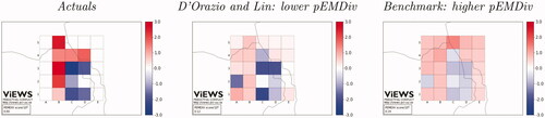
Third, we included the Greene et al. (2019) pseudo-Earth Mover Divergence—pEMDiv. pEMDiv is a network-based, context-sensitive performance metric that nests Earth Mover Distance calculations while simultaneously allowing mis-calibrated predictions as well as asymmetric distance calculations. pEMDiv thus solves the problem of incorporating asymmetric movement costs, and rewards models that produce good but imperfect temporal and spatial approximations even when they fail to hit the target exactly. Predictions are rewarded according to whether they place predicted mass closer in space and time to the actual values they are attempting to forecast. Figure 1 exemplifies the computation of pEMDiv for selected cells based on different sets of predictions for December 2020, s = 2. PRIO-GRID cells are colored according to the prediction; red shades indicate an increase in fatalities, blue shades a decrease. Assuming predictions are identical to the actuals (left panel) pEMDiv equals 0—no energy is needed to move the mass of prediction closer to its actual locations. A low pEMDiv is assigned to predicted changes in fatalities that are close in space to the observed values. For example, the model by D’Orazio and Lin (central panel) correctly predicts de-escalation in grids C1-D1 and C3-D3, and escalation in grids B2-B3, although it under/over-predicts changes in the other grid-cells. The benchmark model (right panel) performs quite well in predicting negative changes in C1-D1 and C3-D3 but is moderately wrong with everything else. For instance, the large over-prediction in the benchmark for column E is far from where escalation actually occurred (e.g. column A). Across all 25 cells, the benchmark requires more “earth movement” and is thus assigned a higher (worse) pEMDiv score than the D’Orazio and Lin model.

Figure 1. Example of pEMDiv (10⁶ scale) computation for selected PRIO-GRID cells for October 2020, using predictions from D’Orazio and Lin (center) and the benchmark model (right) compared to the actuals (left).

In the main text of this article, we report evaluation metrics for the future (October 2020–March 2021; “task 1”). In the Supplementary Appendix, we report the same metrics for the test set (January 2017–December 2019), “task 2”). The evaluation for each task has different advantages and disadvantages. The test set can be sensitive to over- or under-fitting and to data leakage that true future predictions safeguard against. However, the test set has much more actual data to compare against, as the prediction for each step ahead can be compared against all 36 months in the 2017–19 window. The true future set solves the problem of over- or under-fitting, but as it relies on only six months of data for the evaluation, it may be more sensitive to random fluctuations, such as extensive spikes up or down in the number of fatalities.

Summary of Main Evaluation Metrics

Figure 2 summarizes all the model contributions’ performance across the main metrics in a parallel coordinates plot for s = 2 (October 2020). The error is smaller when going from top to bottom of the axis so that the best models lie at the lower end of the graph. As it will be clearer in what follows, we chose to present the evaluation for s = 2, as the predictive task for the true future appears to be more challenging in October 2020 than at the end of the forecasting horizon (s = 7). The Supplementary Appendix reports the evaluation scores and figures for s = 7. In addition to the individual contributions, we present results for the benchmark model (see Hegre, Vesco, and Colaresi 2022), a dumb no-change model predicting no change uniformly across the forecasting window, and an ensemble of all contributions (see Section ‘Scoring the Models Together: An Ensemble of Forecasts’).

Figure 2. Parallel coordinates plots for the main metrics in the True future set (task 1), for s = 2. pEMDiv scores are reported in the scale 10⁹.

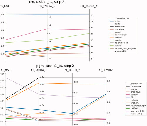
The performance differs by metric. At the cm level, all models perform better than the benchmark (black line) across all metrics. The model by Randahl and Vegelius has the lowest MSE, beating the weighted ensemble by a narrow margin, and immediately followed by Mueller and Rauh, and then Ettensperger. The weighted ensemble of all model contributions (see Section ‘Scoring the Models Together: An Ensemble of Forecasts’) performs only slightly worse than the best individual contribution, according to MSE. Models by Chadefaux and Malone present the best TADDA scores at cm, although all models at the cm level are out-performed by the no-change model according to TADDA. This suggests additional work still needs to be done to improve our understanding of changes in fatalities across space and time.³

At the pgm level, MSE and TADDA scores are considerably lower than at the cm level due to the higher proportion of zeros. The model by D’Orazio and Lin presents the lowest MSE for the true future partition as well as the test set, immediately followed by Radford and Lindholm et al. and closely approached by the weighted ensemble of all contributions. The models by Fritz et al., D’Orazio and Lin, Chadefaux, and Radford rank the best for pEMDiv. The models by D’Orazio and Lin 2022 and Fritz et al. 2022 present the best TADDA scores, outperforming the no-change model according to TADDA1.

Interesting variations in performance are found according to the unit of analysis: for example, the model by D’Orazio and Lin performs quite poorly at cm but ranks the best across all metrics at the pgm level. As the authors suggest, this may indicate that the latent information contained in the dependent variable—which their models rely on—plays a primary role in predicting (de-)escalation at the sub-national level, whereas exogenous variables are more important to forecast changes at higher levels of spatial aggregation.

Variations in performance are found also over time, although the ranking of the models remains quite steady along with the forecasting window. The weighed ensemble performs better for s = 7 than s = 2, beaten only by a narrow margin by Ettensperger at cm and D’Orazio and Lin at pgm (see Supplementary Appendix, Section C).

To give an overview of how performance varies for different steps ahead, Figure 3 shows how MSE changes along the forecasting horizon. The underlying boxplots report the distribution of the actual realizations of conflicts for each step (month ahead) in the October 2020–March 2021 period. The outliers for s = 6 correspond to the secession conflict in Tigray between the Ethiopian government and the Tigray People’s Liberation Front (TPLF) that reignited in November 2020, causing over 1,300 fatalities (Pettersson et al. 2021) in a single month.

Figure 3. MSE for each step (month ahead) relative to the predictions for the true future (Task 1), at the cm (left) and pgm (right) level. The boxplots refer to the actual realizations of conflicts for each month in the October 2020–March 2021 period. The black dot represents the mean with all observations included, the dashed line is the mean with zero changes excluded, the red line is the median.

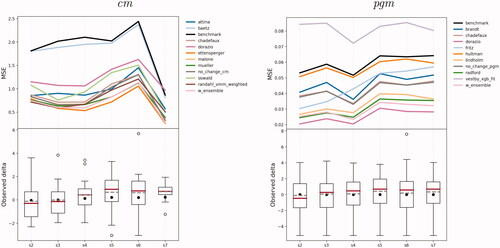
On average, both cm and pgm models’ performance tends to deteriorate along the forecasting horizon, in particular at the pgm level. The further into the future, the harder is the forecasting problem, as one would expect. This gradual deterioration is less clear at the cm level.

This reflects that there is much less data to evaluate against at this level, so individual events influence performance considerably. In particular, the lower performance in February 2021 (s = 6) corresponds to the abrupt escalation of violence in the Tigray region that month, as well as an upsurge in fatalities in Mali, where the government remains challenged by the pro-al-Qaida alliance JNIM. Simultaneously, there was a strong de-escalation of violence in Mozambique after security forces attacked a militant base in Mocímboa da Praia district. Since changes in these three countries dominate fluctuations in all other countries, our evaluation metrics for the true future are very sensitive to this handful of cases. Our metrics for cm predictions for the test set show the same gradual deterioration in predictive performance over time (cf. Table 2).

Table 2. Ensemble scores by step (months into the future), for True future set (task 1) and Test set (task 2), and for cm (top) and pgm (bottom).

Step	Task 1: true future (October 2020–March 2021)				Task 2: test set (2017–2019)
cm	MSE	TADDA1	TADDA2		MSE	TADDA1	TADDA2
2	0.746	0.488	0.596		0.504	0.371	0.419
3	0.600	0.407	0.491		0.551	0.379	0.422
4	0.591	0.391	0.488		0.579	0.394	0.436
5	0.824	0.520	0.627		0.548	0.381	0.429
6	1.134	0.507	0.600		0.573	0.386	0.429
7	0.277	0.331	0.418		0.599	0.400	0.447
sc	0.695	0.441	0.537		NaN	NaN	NaN
Step	Task 1: true future (October 2020–March 2021)				Task 2: test set (2017–2019)
pgm	MSE	TADDA1	TADDA2	PEMDIV	MSE	TADDA1	TADDA2	PEMDIV
2	0.025	0.026	0.028	0.228	0.028	0.039	0.045	0.230
3	0.028	0.031	0.033	0.681	0.025	0.038	0.043	0.174
4	0.023	0.029	0.032	0.283	0.026	0.038	0.043	0.183
5	0.034	0.036	0.038	1.037	0.026	0.038	0.044	0.188
6	0.033	0.030	0.033	0.160	0.026	0.038	0.043	0.144
7	0.032	0.033	0.036	0.389	0.025	0.038	0.044	0.144
sc	0.029	0.031	0.034	0.045	NaN	NaN	NaN	NaN

By and large, pgm models show a similar deterioration in performance along the forecasting window, but many models improve performance in s = 4 (December 2020), characterized by a widespread increase in violence. The better predictive performance of pgm models in s = 4 as well as the trends observed at cm seems to suggest that models are generally better in predicting positive than negative changes in fatalities.

On average across all steps, cm models by Mueller and Rauh, Ettensperger and Chadefaux and pgm models by D’Orazio and Lin and Radford are confirmed as the best performers for both the test partition (2017–2019) and the future set (see Supplementary Appendix, Section C,D). The model by Chadefaux performs very well according to TADDA also at the pgm level. This suggests that the models do not overfit for the test set, with the exclusion of the benchmark model whose performance deteriorates substantially for the true future. Notably, the model presented by Lindholm et al. at the pgm level ranked quite low in the test set, but is one of the best performers for the true future, especially according to MSE and MAL (See p. 16). This set of scores is consistent with a model that appeared to under-perform for the test set but did learn how to generalize the patterns in the historical data relatively well.

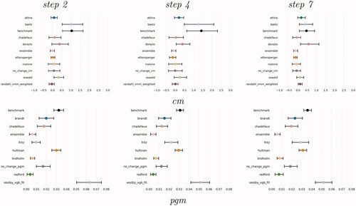
As differences in model performance between the future set and the test set might be due to sampling variability, Figure 4 presents the average difference between the MSE score of each model and the MSE of the best performing model in the test set that is, Mueller and Rauh for the cm and D’Orazio and Lin for pgm level (Supplementary Appendix, Section B). Negative values represent lower MSE in the true future set as compared to the best performing MSE in the test set. The Figure visualizes the uncertainty related to forecasts by plotting confidence intervals. The 95% confidence intervals are obtained by bootstrapping the vectors of predicted and observed values in the future set 1,000 times and computing the difference between the MSE of each contribution and the MSE of the reference model for all bootstrapped pairs. At the cm level, in particular, we see small differences and intervals that cross zero, denoting that several models have avoided overfitting the training data or epiphenomenal signals and have similar generalization performance to the model identified as best in the test set. This helps increase our confidence that if these models were deployed to make predictions in the field, their future error rates would be similar to the estimated error rates from the test set. The ensembling approach by Ettensperger, the ensemble of all contributions, and the weighted Markov Model presented by Randahl and Vegelius are the closest in MSE to the score of Mueller and Rauh. The models by Chadefaux and Malone also present very similar MSE scores to the one of Mueller and Rauh, but the uncertainty around the metric is relatively higher. The MSE score of the benchmark and the model by Bätz, Klöckner, and Schneider show the highest distance to the one of the best model. These results do not change considerably along the forecasting horizon, although the uncertainty of the metrics tends to increase for s = 4. At pgm, the model by Radford and the one by Lindholm et al. as well as the ensemble of all models present the closest MSE to the one of D’Orazio and Lin. The model by Fritz et al. also has quite a similar MSE than D’Orazio and Lin for s = 2 but the difference increases further ahead into the future.

Figure 4. Difference in MSE, True future set (task 1), between each model and model performing best in the test set (task 2), cm (top) and pgm, bottom. The bars represent 95% confidence intervals obtained by bootstrapping the vectors of predictions and actual values 1000 times and computing MSE for each bootstrapped pair. The best models, Mueller and Rauh (cm) and D’Orazio and Lin (pgm) are not shown.

Scoring the Models Together: An Ensemble of Forecasts

One of the goals of the competition was to leverage multiple and diverse prediction approaches toward the same target to increase forecasting accuracy. The “wisdom of the crowd” suggests that the aggregation of diverse models provides a more precise forecast than its single components (Page 2018). The diversity prediction theorem is key here—a diverse group of problem solvers is better than a homogeneous group with the same average performance (Page 2007, 209), so that the more diverse the forecasting models, the better the aggregated prediction.

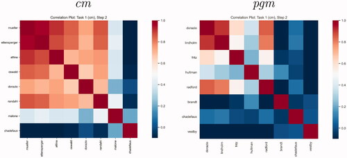
For an overview of the similarities and disparities among contributions, Figure 5 shows the correlations between predictions from every model at the cm and pgm levels. The correlation map shows that most models at the cm level yielded predictions with a moderate correlation. Malone and Chadefaux are more distinct models compared to the average. At the pgm level, Radford; D’Orazio and Lin, and Lindholm et al. exhibit a modest correlation, while Vestby et al., Chadefaux; and Brandt et al. are more diverse.

Figure 5. Plots of correlations between predictions from all contributed models, forecasts for October 2020, cm (left) and pgm (right).

Computing an ensemble of all predictions provides an intuitive representation of the wisdom of the crowd. Table 2 presents the MSE and TADDA score of an ensemble of the contributions, weighted by the inverse of MSE for task 2 (2017–2019).

In line with the diversity prediction theorem, the average performance of the ensemble across all steps is better than the average single contribution.

Gathering a crowd of diverse models has generated a global forecast that improves upon the vast majority of individual predictions, although the best individual models at both levels of analysis score better than the ensemble of contributions. This might to some extent reflect the relatively poor performance of some models in the test set, such as that of Lindholm et al., which are correspondingly assigned a lower weight in the ensemble than would be optimal for the true future. The ensemble predictions are heavily influenced by the average prediction: if almost all models predict an increase in fatalities where there was a decrease, the ensemble is likely to predict an increase. Even though the best model may have correctly identified the negative trend, its individual contribution is compensated by the power of the crowd. This reiterates the importance of having both diverse and good predictions to maximize ensemble performance. To further improve the state-of-the-art, new innovations for diverse, accurate predictions will need to be uncovered.

Additional Metrics to Identify Diverse Contributions and Other Valuable Traits

We have considered a comprehensive set of metrics in line with the overarching goal of the competition (see Hegre, Vesco, and Colaresi 2022) and the evaluation criteria presented in Section ‘Evaluation Procedures’.

Since some of these metrics were not specifically announced to participants in advance, we discuss them separately in the evaluation below.⁴

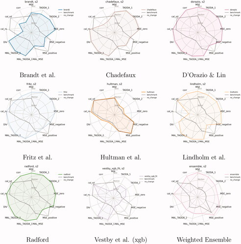
Figures 6 and 7 summarize all of them for s = 2) and indicate the relative strengths and weaknesses of the models. The same figures are replicated in the Supplementary Appendix for s = 7. There is one radar plot for each contributed model. Each radial axis represents one metric, normalized on a 0–1 scale. All axes are scaled so that the line for the best-performing model reaches the outer ring, and the poorest model is placed at the inner ring.⁵ Models that do well on many metrics, then, have a large shaded area, while smaller areas represent less-performant models.

Figure 6. Summary of evaluation metrics by model (cm), True Future set (Task 1), predictions for October 2020 (s = 2). All metrics are normalized; MSE and TADDA scales are inverted so that the further away from the origin the better the model’s performance.

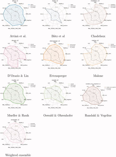
Figure 7. Summary of evaluation metrics by model (pgm), True Future set (Task 1), predictions for October 2020 (s = 2). All metrics are standardized; MSE and TADDA scales are inverted so that the further out from the origin, the better the model’s performance.

A comparison with the Figures in the Supplementary Appendix reveals that models perform better for s = 7 than for s = 2. This may suggest that the prediction task is more challenging for October 2020 than for March 2021, where the change in fatalities is more homogeneously positive across locations. An assessment of the evaluation metrics across all time-steps, in fact, reveals a higher degree of complexity and points to a non-linear deterioration of the model’s performance over time.

Each sub-figure includes the scores of two reference models: a benchmark model distributed by the ViEWS team to all participants a few months before their submission deadline, and a no-change model. The benchmark is summarized in the introduction to this Special Issue (Hegre, Vesco, and Colaresi 2022), and the no-change model simply predicts no change for all units of analysis. The Figure also includes the scores for the weighted ensemble of all contributions.⁶

First, based on an ensemble where all models were weighted equally, we computed the Model Ablation Loss (MAL), a metric aimed at rewarding models’ unique contributions to the “wisdom of the crowd.” MAL is obtained by observing how the performance of the ensemble of the predictions varies when dropping a specific model from it. Specifically, we define MAL as the change in the ensemble MSE determined by removing the model from that ensemble: (1) $$MA{L}_m^{\mathit{MSE}}=-(MS{E}^{\mathit{full}}-MS{E}_m^{\mathit{abl}})$$(1) where m is the model, MSE^full is the MSE for the ensemble with all models, and $MS{E}_m^{\mathit{abl}}$ the score for the ensemble without model m. We also derive MAL based on TADDA scores. When MSE increases as a result of the model’s removal, the contribution of that model is positive—removing the model from the ensemble harms the predictive performance. If MSE (TADDA) decreases, the ensemble performs better without that model.

Figure 8 shows the MAL values for different steps ahead. The metric is positive—the dot is to the right of the central line—if the ensemble without model m is worse than the ensemble including it, meaning that the model contributes positively to the predictive performance.

Figure 8. MAL—losses from removing individual models from the unweighted average ensemble. Dots are colored according to the MSE of the models on their own. Models that improve the predictive performance of the ensemble have positive scores and are plotted to the right of each panel.

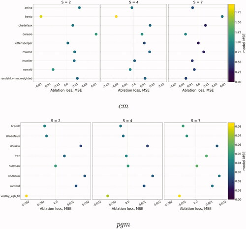
On average, Mueller and Rauh, Chadefaux, and Malone have the best MAL scores at the cm level. The model by D’Orazio and Lin presents the best MAL score for s = 2 while the model by Bätz, Klöckner, and Schneider adds a significant contribution to the ensemble for s = 7. The contribution of each individual model to the ensemble drops considerably when predicting far ahead into the future (for March 2021), and five out of nine cm models have a non-positive MAL for s = 7. The model by Oswald and Ohrenhofer has a slightly negative contribution in the future set despite presenting one of the best MAL scores in the test set.

The time trend is less clear at the pgm level, where the models by D’Orazio and Lin and Lindholm et al. display the best average MAL score along the entire forecasting horizon. The model by Fritz et al. scores positively for s = 2 and s = 7, but its contribution drops for the other steps. As Figure 8 makes clear, novel insights and unique contributions to the ensemble may come from models that do not have the best MSE or TADDA scores individually.

Next, as models’ diversity can contribute to improve the ensemble forecast, we complemented our evaluation metrics with a measure that approximates models’ contribution to diversity (Equation 2(2) $$\frac{1}{n}\sum _{i=1}^N\left[\frac{1}{M}\sum _{m=1}^M\left(p_i^{(M)}-p_i^{(e)}\right){}^2\right]$$(2) ). Following the diversity prediction theorem, we compute the diversity of the ensemble as: (2) $$\frac{1}{n}\sum _{i=1}^N\left[\frac{1}{M}\sum _{m=1}^M\left(p_i^{(M)}-p_i^{(e)}\right){}^2\right]$$(2) for m models in $[1,2\dots M].$ $p_i^{(e)}$ is the ensemble prediction; $p_i^{(M)}$ is the individual prediction from model M across n units at pgm or cm (adapted from Page 2007).

To understand how different models enhanced or reduced the diversity of the ensemble across all predictions, we calculated the contribution of each model to the crowd’s diversity in the same way we computed MAL (1)(1) $$MA{L}_m^{\mathit{MSE}}=-(MS{E}^{\mathit{full}}-MS{E}_m^{\mathit{abl}})$$(1) , but replacing MSE with the diversity score as defined above. These scores are visually summarized in Figures 6 and 7.

At cm, the greatest contributions to diversity come from the models presented by Bätz, Klöckner, and Schneider, and to a lesser extent from D’Orazio and Lin. Models by Hultman, Leis, and Nilsson, Vestby et al., and Lindholm et al. achieve the highest diversity score at pgm, along with the benchmark model. Particularly at cm, the most diverse models correspond quite well with those performing poorly according to MSE. As ensembles reflect the diversity of the crowd of models, these trends may explain why the ensemble of the contributions is out-performed by the best individual models. Constructing an ensemble that step-wisely evaluates the performance and removes the poor-performing models might therefore help improve the prediction of the crowd.

Building on the participants’ feedback, we also introduce some evaluation metrics that take the forecasting distribution into account. Many participants in the competition have correctly pointed to the importance of evaluating the distribution of forecasts other than point predictions (Hegre, Vesco, and Colaresi 2022). Evaluating the distribution of forecasts would avoid the problem of extracting a single parameter, such as the mean from a distribution, which is a sub-optimal representation of the vector of predictions, particularly for non-normal distributions like the one of interest here (Lindholm et al. 2022). For the target of this competition, models should be rewarded for their ability to predict at the ends of the distribution where a change actually occurs, other than in the neighborhood of the distribution mean, which is close to zero.

Calibration

A good prediction model can rank observations correctly so that the cases where we observe the largest increases in fatalities correspond to those where the predicted increases are the largest. In addition, however, models should also be well-calibrated—on aggregate, they should predict the right amount of change in violence, and also have a variance that reflects that of the actuals.⁷ We compute two measures: $\mathit{cal}\_m,$ which is the squared difference between the predictions mean and the mean of the actuals, and $\mathit{cal}\_\mathrm{sd},$ which is the squared difference between the standard deviation of the predictions and the standard deviation of the actuals.⁸ Scores are reported in Figures 6 and 7. A $\mathit{cal}\_m$ score of 0 would indicate a perfect prediction.

Both cm and pgm models are on average miscalibrated, as suggested by the magnitude of $\mathit{cal}\_m$ being >0. The models tend to be poorly calibrated for s = 2 (October 2020), while the scores improve for s = 7 (March 2021). Predictions at both cm and pgm are on average close to the observed mean, but less so to the true variance of the predictions. The best $\mathit{cal}\_\mathrm{sd}$ scores at the cm level are those by Oswald and Ohrenhofer; Attinà, Carammia, and Iacus; Ettensperger; and Mueller and Rauh, reiterating that ensembles of models like those by Ettensperger and models that can capture early signals of tensions, such as those by Mueller and Rauh and Oswald and Ohrenhofer can lead to measurable performance gains even on less traditional metrics.

At pgm, models by Fritz et al., Hultman, Leis, and Nilsson, Lindholm et al., and Vestby et al. present the best $\mathit{cal}\_\mathrm{sd}$ scores, suggesting that these specifications could usefully learn patterns that are not necessarily obvious from comparing MSE or other metrics. The calibration metrics also suggest that the poorer performance of some of the models might simply be the by-product of bad calibration.

Conditional MSEs and Correlation

As conflicts fortunately are rare events, evaluation metrics are heavily influenced by the performance for all cases with zero change. To give a simple measure of how models rank in predicting changes where they do occur, we compute conditional MSE and correlation scores. Conditional MSEs represent models’ precision across different subsets of the target. Each measure indicates the models’ contribution to their MSE, conditional on the value of the outcome—positive, negative or close to zero.

Correlation between the vector of predictions and the vector of the actuals can be thought of as a rescaled measure of co-variance and gives a simple representation of how predictions are linearly related to the outcome. We compute the correlation for the full sample (presented in Figures 6 and 7) as well as partial correlations conditioned on the value of Y being positive, negative or close to zero. Partial correlation and MSEs embrace the precision component of accuracy, which complements standard metrics by taking into account how good models are in predicting actual changes. In Figure 9, we plot conditional MSEs (x-axis) against the partial correlation between Y and $\widehat{Y}$ (y-axis) for s = 2 (scores for s = 7 are reported in Supplementary Appendix).

Figure 9. Scatterplots of conditional MSEs (x-axis) against the partial correlation between Y and $\widehat{Y}$ (y-axis) for s = 2, True future set. Scores are defined with respect to the value of the outcome Y being equal, greater or lower than ϵ (0.048). Shapes correspond to different outcome values; dots stand for outcome values close to zero; upward triangles represent cases of escalation, and downward triangles those of de-escalation. To make dots visible, axes’ range differs for the near-zero subset (left column).

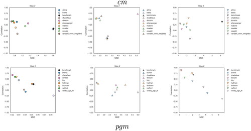
To make visualization easier around the zero value, we define each subset of the outcome for both MSE and correlation with respect to ϵ = 0.048, that is, for $y<-ϵ,$ $-ϵ<y<ϵ,$ and $y>ϵ.$ This mitigates the overlapping of dots around the zero value and enables us to compute the partial correlation for the subset of the sample where Y approximates but is not exactly equal to zero. Dots on the top left corner of the graphs represent models that have both high correlation and low MSE.

As the labels on the x axis in Figure 9 make clear, near-zero observations (left plots for cm in the first row, and pgm in the second row) have a much lower contribution to the MSE compared to the observations where there were actual positive or negative changes. For the observations with changes >0.048 (central columns for cm, first row, and pgm, second row), with very few exceptions, the correlation and MSE tell similar stories across the models. Models that predict changes in absolute terms that are closer to the actual values (and thus have a lower MSE) also tend to have a higher covariance with the true values (higher correlation) on that set of observations. This does not have to be the case. For example, the cm model by D’Orazio and Lin has a much higher covariance with the positive changing observation than one would expect from the MSE alone. Since our true future set is so short, this can be due to random variation. But this can also happen when a prediction is mis-calibrated. In absolute terms, that mis-calibrated model might drastically over or under-predict changes of a particular type, but still be useful as an index, such that high values of the prediction index lead to higher changes of interest. In addition, we can see that while changes are indeed more difficult to predict than no-change—one of the factors motivating this competition—almost all models improve on the MSE and correlation of the benchmark model specifically for these observations of upward and downward shifts in fatality levels at both cm and pgm levels. Also, both cm and pgm models are relatively better at predicting positive rather than negative changes, as shown by the clear cluster of upward triangles with at least moderately high correlation and low MSE in the central column of Figure 9.

At cm, predictions by Mueller and Rauh (green) and Ettensperger (orange) show the best partial correlation and MSEs for all values of the outcome. Randahl and Vegelius (brown) perform particularly well when predicting positive changes in fatalities, whereas Malone (light orange) and Chadefaux (light brown) have among the best scores for negative changes. These results overall suggest that sophisticated modeling approaches that work on the latent information contained in the outcome variable, for example by improving the identification of temporal/spatial trends, may reduce the costs of errors in observations where changes are occurring (up or down). At pgm, D’Orazio and Lin (pink) and Lindholm et al. (light orange) have the lowest partial MSEs and highest correlations across the different subsets of the target, especially for the negative one. The model by Radford (light green), which tends to predict a decrease in fatality if there exist non-zero casualties at the initial time step (Radford 2022), performs particularly well for predicting negative changes. Predictions by Hultman, Leis, and Nilsson (orange), which integrate the moderating effect of Peace Keeping Operations on ongoing conflicts, rank among the best for the positive sub-sample.

Visualizing the Prediction Errors

We can learn even more from the predictions by mapping and plotting the types of errors each is making. In Figures 10 and 12, we plot the prediction errors in map form for October 2020 (s = 2) relative to August 2020. Prediction errors are the simple difference between the forecasts and the actual observations.⁹

Figure 10. Error in predictions, Future set, cm, predictions for October 2020, s = 2.

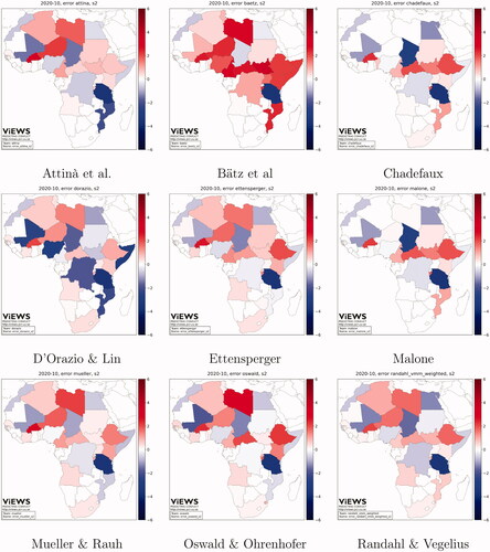
Models at cm level show a tendency to under-predict the change in fatalities (blue shades) in Tanzania, Chad, and Egypt. Almost every model predicts a higher positive change in fatalities than the actual (red shades) in Libya, Algeria, Burkina Faso, Ethiopia, and Central African Republic. Models are more distinct in their predictions for Nigeria, Mali, and Somalia, although the errors of some cm models show very similar patterns, such as Mueller and Rauh and Oswald and Ohrenhofer, or Malone, and Chadefaux.

Pgm models (maps in Figure 12) differ more substantially than cm ones. Brandt et al. and Hultman, Leis, and Nilsson show a slight tendency to over-predict change in fatalities (brown shades). With few exceptions, all models under-predict (green shades) the change in violence in central Mali and in the area of the Lake Chad basin, whereas they over-predict violence in the south and central Somalia and at the border between Tanzania and Mozambique. Predictions are more diverse for the Anglophone region of Cameroon and the northeast of Democratic Republic of the Congo (DRC).

To complement the maps of prediction errors, and visualize where and when the contributions perform well and where/when they are less accurate, Figures 11 and 12 show an adapted version of the model criticism plots (Colaresi and Mahmood 2017) for October 2020 s = 2, at the cm and pgm level.

Figure 11. Model criticism plot, Future set, cm, Predictions for October 2020.

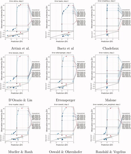
Figure 12. Model criticism plot, Future set, pgm, Predictions for October 2020.

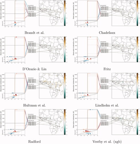
The plots visualize discrepancies between the observed continuous outcome and the corresponding predicted value. The x axis plots the predicted change $\Delta \widehat{y};$ the y axis rank-orders the forecasts from lowest to highest to make the observations visible. To ease the comparison against observations, the dots are colored by the observed value; blue dots indicate that the actual observed change in BRDs was negative, while red stands for an actual increase. In a perfect model, all blue dots would be on the left-hand side of the x-axis, all red dots on the right-hand side, and all dots on the zero line would be white (no-change). Blue dots toward the right, then, indicate that the model predicted a positive change in fatalities where there was an actual decrease; red dots on the left side conversely indicate a predicted negative change whereas the true delta value was positive. The more intense the shade of the color, the larger the actual change in fatalities. Dark-shaded dots should therefore lay toward the extremes of the x-axis. To ease the visualization of the grid-cell locations, pgm plots are complemented by error maps that show the simple difference between the predicted and actual value.

Cm models by Chadefaux, Malone, and Randahl and Vegelius, as well as pgm models by Brandt et al. and Chadefaux have few large under-predictions (the predicted change is lower than the actual) or over-prediction (the predicted change is higher than the actual).

Cm models by Bätz, Klöckner, and Schneider, D’Orazio and Lin, and Attinà, Carammia, and Iacus display considerably higher distances between predicted and realized values, especially for their over-predictions. These impressions are related to the variance in predictions, as seen in the prediction maps presented in Hegre, Vesco, and Colaresi (2022).

As displayed in Figure 10, almost all cm models over-predict the change in fatalities in Lybia and Burkina Faso and under-predict the changes in Tanzania and Egypt. Mis-predictions of Tanzania are notable as most of the models miss the outbreak of conflict in Tanzania as the escalating violence perpetrated by IS in the neighboring Mozambique spread across the border in October 2020.

Pgm models by Radford and D’Orazio and Lin and to some extent by Fritz et al. display similar error patterns, while the Xgboost model by Vestby et al. has a tendency to predict negative changes in fatalities where positive changes occurred. Models by Brandt et al. and Radford also predicted a negative change in fatalities in the Sinai peninsula, missing the occurrence of one battle-related death in October 2020.

Summary of the Models’ Performance

The ranking of the models across various metrics and criteria point to the potential of data-driven algorithms that learn how to generalize the spatio-temporal dependencies in the observed data. This is particularly true at the pgm level (e.g. D’Orazio and Lin, Radford, Chadefaux, Figure 7). Models that leverage the flexibility of machine learning and do not superimpose any constraints to the functional form perform better than models that rely on more rigid specifications. At the same time, unique insights come from the introduction of contextual variables that can help to predict early signals of escalation (e.g. Bätz, Klöckner, and Schneider, Fritz et al., Oswald and Ohrenhofer) as well as features that compensate for the tendency of over-predicting positive changes in locations with a strong legacy of violence (e.g. Hultman, Leis, and Nilsson). Ensemble approaches like the one presented by Ettensperger and Randahl and Vegelius, Markov models like those by Lindholm et al. and Randahl and Vegelius, and techniques that extract textual information to detect early tensions, like the model specified by Mueller and Rauh, rank particularly high.

A comparison of the models’ performance for s = 2 (Figures 6 and 7) with that for s = 7 reported in the Supplementary Appendix suggests that almost all models perform better for s = 7 than for s = 2 (see Figure C-6 and C-7 in Supplementary Appendix). This is quite opposite to the trend observed in the test set (see Supplementary Appendix, Section D), for which most models, especially at cm, perform better for a shorter time horizon. As the evaluation for the test set relies on a higher amount of data that makes it more accurate than the evaluation for the true future, trends in predictive performance observed for the future set are likely driven by random fluctuations in the conflict data rather than by a genuine improvement of the models’ abilities for longer time horizons.

Figures 6 and 7 and the evaluation of the various metrics we have presented also show that models have different strengths—some do well on the main metrics, whereas others do well on subsets of observations, in a diversity perspective, or are well-calibrated. This suggests that a promising approach might be to feed data-hungry, highly flexible, machine learning-inspired model representations with theoretically sound features, and gather the outcomes of different model specifications and algorithms into an ensemble to boost performance.

After independent assessment of the models and consideration of the main evaluation metrics (‘Section Main Evaluation Metrics’: MSE, TADDA, pEMDiv) and criteria illustrated in these sections, the scoring committee ranked the contributions to the competition. The following section presents their evaluation.

Scoring Committee’s Summary

In line with the evaluation criteria defined for the competition, the scoring committee (SC) gave different awards for particular features of the submitted prediction models. The SC collapsed the criteria for the contest into three main ones: predictive accuracy, originality, and transparency/replicability. Due to the different prediction problems set up for the contest (at cm and pgm levels) and team participation at different levels, the SC selected two winners for each of the three awards, one for each prediction problem.

Award for Predictive Accuracy

The award for predictive accuracy is based on the scores computed for each contribution by the ViEWS team (Section ‘Evaluation of the Contributions’). As outlined in this report, the team produced MSE and TADDA scores for each contribution and each prediction problem (Section ‘Main Evaluation Metrics’: MSE, TADDA, pEMDiv). MSE is a frequently-used metric to estimate model fit, and its application to prediction problems is straightforward. TADDA is a new metric designed by the ViEWS team. While we share the motivation for this new metric—consideration of direction and magnitudes of errors—we also note that its application in the contest is somewhat problematic. In particular, with the parametrization used for the evaluation, in the TADDA score, no model can outperform the no-change model predicting “no change in violence”. This means that a model with predictions very close to a constant no-change model would be preferred if evaluated according to this score, which the SC did not consider to be a good choice.¹⁰ Therefore, the SC decided to base their evaluation entirely on the MSE scores (setting aside pEMDiv scores as they are unique to the pgm level).

Among MSE scores for the cm prediction, Ettensperger leads the group with an average MSE of 0.656 over the six-time windows, followed by Mueller and Rauh with an average of 0.732.¹¹

In the pgm prediction problem, D’Orazio and Lin is the clear winner with an average MSE of 0.025; Radford is runner-up with an average MSE of 0.031.¹²

Award for Originality

The award for originality is given to those models that make an independent contribution when using the ensemble of all models for prediction. The SC believes that this type of evaluation is extremely interesting and relevant and that its addition to the contest by the ViEWS team is very useful. MAL scores were computed again based on MSE and TADDA scores. For the reasons explained above, the SC based their evaluation only on the MSE-based MAL scores, taking again the average over the six-time windows. Larger (more positive) scores indicate that ensemble performance decreased after a model is removed, which signals the high originality of the respective model. The SC, therefore, rewarded models with higher scores.

For the cm prediction problem, the Malone and Chadefaux models score best for average MAL.¹³

For the pgm prediction, the Lindholm et al. and D’Orazio and Lin models seem to be making the best independent contributions to the ensemble.¹⁴

Award for Transparency and Replicability

Highly ranked contributions for transparency and replicability were based on several dimensions. As codes for all contributions were submitted, team contributions were seen as equally satisfactory on the point of “availability of codes” to rerun all analyses. Beyond code availability, the SC considered whether the utilized data were publicly available data sources, as proprietary or expensive data sources add additional burdens to replication both of the forecasting exercise here but also in applying the proposed approach in future applications. Submissions that were as limited as possible in ad-hoc manual or researcher-overseen choices in pre-processing of the data, selection of features, and/or tuning of models also scored higher in this category. Motivated by replication in future contexts, we see value in an approach that requires less expert knowledge or data-specific hand-tuning required for the approach to carry forth elsewhere. Finally, contributions that had computational burdens that were within the realm of reasonable research resources (e.g. all steps of the forecasting exercise could be performed at a university computer or cluster system) were also scored higher.

We highlight the approach by Oswald and Ohrenhofer (at the cm level) for its perceived ease of replication, due to the use of available R packages, usage of open-source data—including new information gleaned from Wikipedia statistics—and the simple set-up. Likewise, we see Chadefaux’s (at both cm, pgm levels) contribution, which uses a time warping algorithm, as high in transparency and replicability given the ease of calculations (splits into sequences and calculations of distances) and openness to parallelization, while simultaneously using standard available data.

Concluding Remarks and Recommendations

All in all, the prediction competition clearly has contributed to the challenging task of predicting change in fatalities in armed conflict. First, the competition and the accompanying publication provide a helpful glimpse at the state-of-the-art of conflict forecasting. Second, approaches that outperform simple “no-change models” are available at both cm and pgm levels; third, individual competition efforts can be combined to improve the predictive accuracy of the ViEWS benchmark model. Highlights of novel aspects of individual contributions included, but are not limited to, usage of new, open-source data (e.g. Wikipedia stats from Oswald and Ohrenhofer), timely incorporation of COVID effects (Bätz, Klöckner, and Schneider), new methodologies, such as dynamic time warping models (Chadefaux) and incorporation of prediction uncertainties in final analyses (Lindholm et al.). Fourth, model performance in general decreases non-linearly the longer we predict into the future (with caveats).

We have evaluated the models both for true future predictions (October 2020–March 2021) and for a test set (January 2017–December 2019). For the test set, we could juxtapose 36 “time-shifted” predictions, but for the true future, we only had one. Accordingly, the evaluation of the true future was more sensitive to individual events, such as the flaring up of fighting in the Tigray province in the Fall of 2020. Fortunately, the ranking of the models relative to each other does not change much between the two tasks. This shows that cross-validation approaches provide relatively accurate model performance rankings even for a volatile phenomenon, such as conflict prediction, wherein expectations might suggest different evaluation periods lead to vastly different relative outcomes. Overall, we believe that the competition has vastly stimulated progress in forecasting political violence and helped identify cutting-edge research moving forward.

Yet, there are also some lessons to be learned from this exercise. One consideration regards the types of metrics used to evaluate predictive accuracy. The explicit selection of the log change in the evaluation metric risks ignoring the magnitude of the conflict. In addition, due to the $\text{log}\hspace{0.17em}(y+1)$ transformation, a change from no violence to 10 casualties is the same as the change from 10 to 100 casualties. This may be problematic since it conflates onset and escalation. The classic use of MSE is still a straightforward metric and likewise, takeaways are easy in this sense using this statistic. The MAL statistic has proven helpful for the evaluation of the individual contributions of team models against a whole ensemble of all other models. The TADDA score is well-motivated as an attempt to account for the direction and magnitude of errors. Some models have successfully predicted substantial change in the count of the log number of fatalities per month from state-based conflict, but the TADDA score appears to overly favor the simple “no-change model” in this regard. Perhaps an approach that explicitly separates these different and important dimensions of errors (direction and magnitude) as individual statistics would be more transparent and easier to work with, without making functional form assumptions.

In the spirit of transparency and scalability, we offer a few takeaways and suggestions for future competitions and research on prediction models in general. First, we see the benefits of providing strict policies on data usage, such that sources must be either publicly and/or widely available, to ensure within-competition full replication, as well as replication in other contexts. Second, given the variation in methods, it may prove useful for the competition to standardize the presentation of steps for each method broadly under categories of (a) data and preprocessing, (b) features and model selection, (c) training and validation, and (d) testing. Indeed, this should also be accompanied by an explicit audit trail of all decisions made throughout the project. Third, we see the added benefit of requiring assessments of scalability and sustainability (e.g. whether the project is scalable/usable in other contexts and whether the infrastructure needed for processing has environmental impacts). As it is often difficult to extricate evaluations of whether approaches are boosted primarily through the incorporation of novel data, improved approaches, or other various aspects, we further suggest separating the parts of approaches (a–d) such that they can be independently run; experimentation can be applied to each of the steps to separately evaluate their impacts on the final prediction accuracy.

Since the prediction of changes/direction is even more relevant from a policy-/practitioners-perspective than simply forecasting the probability of conflict occurrence, the development of models focusing explicitly on these harder problems and the implementation of metrics to evaluate such efforts would help to advance the usefulness of conflict forecasting systems for. By the same logic, approaches that heighten predictive accuracy based on conflict history-related features alone are of limited value. These developments may be used in the context of some operational planning, but only if they can be explained with relative ease to non-technical audiences. The usability of such models is further limited since features related to conflict history—for example, the number of fatalities or neighboring conflicts—can hardly be addressed using diplomacy or development cooperation, especially in the context of an ongoing armed conflict.

Future prediction competitions could focus on different distinct dimensions of change regarding the development of armed conflicts: onset, vertical de-/escalation (number of fatalities, events, actors actively involved), horizontal de-/escalation (changes in areas where conflict events happen or where vertical de-/escalation take place) or on the identification of changes in conflict states or phase transitions. In addition, they could be set up to support the development of approaches that can deal with the challenge identified by Bowlsby et al. (2020, 1416) that drivers of political instability are likely time-variant and that related prediction models should be revised and validated on a continued basis. At the same time, we believe that scientific advances in conflict prediction require more attention to the communication of their findings to general audiences. Taking a page from weather forecasting, prediction efforts can benefit from continuous updating, with publicly available data and models including accompanying information, such as assessments of the reliability of input datasets, potential biases, and model assumptions.¹⁵ The overall aim would be to produce easily accessible predictions that can be understood and trusted.

Conclusions

This article has presented results from and reflections on a prediction competition to encourage advances in the forecast of changes in state-based conflicts. An independent scoring committee was formed to evaluate the contributions according to different criteria, including predictive accuracy, uniqueness, novelty, and replicability. Although there is room for improvement in its implementation, we believe that competitions of this sort have immense potential to advance the research frontier both methodologically and theoretically.

We have learned several lessons. First, results from a simple, weighted average ensemble of the contributions show that the overall set of models achieves considerably better performance than the average individual contribution. Highly flexible, data-hungry model representations tend to perform better than sparser, linear models. Ensembling approaches, algorithms that extract textual information from news sources, and specifications that build on theoretically-sound features, all contribute great insights to the crowd of models. The models’ performance does not show a clear trend to deteriorate along the forecasting horizon, although according to some metrics forecasts for s = 7 are surprisingly more accurate than those for s = 2 in the future set. As the opposite is observed in the test set, this deterioration seems to relate to the random fluctuations in conflict trends observed in the October 2020–March 2021 window, rather than to the actual predictive capacity of the models.

Also, a set of varied evaluation metrics is needed to capture different models’ insight and innovations and to reward models’ ability to predict substantial changes where they occur, other than null change where nothing happened. In fact, particularly at the geographically disaggregated pgm level, models are highly affected by the inflation of zeros that drives the MSE down.

Overall, we showed that competitions such as this one are a useful tool to advance the research frontier on complex problems like the prediction of violence and generate new insights, collectively, that would not be present in any individual model.

Acknowledgments

We are grateful to Espen Geelmuyden Rød for his great contribution in developing and launching the prediction competition and his help in the initial stage. We are thankful to the ViEWS team and the participants in the competition for their support. We thank two reviewers for their comments that greatly improved the manuscript.

Correction Statement

This article was originally published with errors, which have now been corrected in the online version. Please see Correction (http://dx.doi.org/10.1080/03050629.2022.2101217).

Additional information

Funding

The prediction competition and the related manuscripts have been funded by ViEWS—ERC Grant n. 694640. ViEWS computations are performed on resources provided by the Swedish National Infrastructure for Computing (SNIC) at Uppsala Multidisciplinary Center for Advanced Computational Science (UPPMAX).

Notes

1 The Online Supplementary Appendix reports the invitation letter that we sent to the participants, including the criteria and metrics that we announced.

2 Both TADDA include $\text{TADDA}{(d=1)}_M^{(1)}$ and $\text{TADDA}{(d=2)}_M^{(1)}$ include a parameter ϵ that serves as a domain-specific, user supplied threshold below which errors in predictions are not penalized. By default, we set ϵ to 0.048, which corresponds to tolerating errors lower than $\mathit{log}(0.048+1),$ i.e. around 5%. Errors in the wrong direction and greater in magnitude than ϵ are assigned an added penalty by TADDA; errors below that value are not penalized further.

3 To avoid confusion, it is possible for models to improve on the no-change predictions theoretically. In fact, at least one model at pgm beats the no-change predictions according to both TADDA1 and TADDA2 in the true future partition for s=2, although no model score better than the no-change baseline for the test set. A few additional models did improve upon the no-change model if squared error is used instead of absolute error in the TADDA calculation. We will build on these experiments in future work.

4 We did, however, announce the general guiding evaluation criteria in our invitation to participate, and mentioned that models would be evaluated through a quantitative as well as a qualitative assessment. The Supplementary Appendix reports the Invitation letter that we sent out to scholars at the beginning of the competition.

5 To achieve this scaling, we have inverted the scale of MSE, TADDA and pEMDiv and adjusted the calibration scores cal_m and cal_sd so that the higher the score, the better the performance.

6 As the MAL and diversity scores are based on the ensemble and could not be computed for it, they were set to 0.5 as default.

7 Theoretically, a model that adequately represents the variance of the outcome is more accurate than models with predictions with much more or much less variance. However, as conflict cannot be measured with certainty, the dependent variable most likely contains some noise. A variance of prediction that is very close to the variance of the actuals can either indicate that the model is very good at reproducing the correct signal from the outcome, but also that it captures the noise contained in the outcome, and therefore a high correspondence between the two variances cannot exclude that the model is over-fitting.

8 Taking the square of the difference assigns the same penalty to over- and under-estimating the variance or the mean relative to the actual values.

9 The actual observations are plotted as Figure 3 in the introduction article (Hegre, Vesco, and Colaresi 2022).

10 Note from the ViEWS Team: After consultations with the competition participants and feedback from the SC, we introduced two versions of TADDA. TADDA2 punishes null predictions when the outcome is not zero relatively more than TADDA1. TADDA1 was used in the previous iteration of the evaluation, and in retrospect TADDA2 would have been a better metric for the specific goal of this competition. However, it is not the case that no model can outperform the no-change model—simply no model presented in the competition did for the test set. The models presented by D’Orazio and Lin and Fritz et al. do outperform the no-change model according to TADDA1 or TADDA2 for some time-steps in the true future partition. In the future, we plan to evolve the TADDA description and implementation to become TaDDA (Targeted Distance with Direction Augmentation) and allow researchers to choose whether to use absolute or squared distance. Here, a few models would beat the no-change model if a $\mathit{TaDD}{A}_2^2$ measure, or a metric with squared distance instead of absolute distance was used.

11 In the test task, the two teams were flipped in MSE scores.

12 The test task resulted in the same top two teams.

13 Test set winners were Oswald and Ohrenhofer and Attinà, Carammia, and Iacus.

14 Test set winner was D’Orazio and Lin.

15 See The Centre for Humanitarian Data’s draft of a Peer Review Framework for Predictive Analytics in Humanitarian Response (https://centre.humdata.org/predictive-analytics/) for more information on standardized documentation and assessments of ethical concerns).

References

- Attinà, Fulvio, Marcello Carammia, and Stefano Iacus. 2022. “Forecasting Change in Conflict Fatalities with Dynamic Elastic Net.” International Interactions 48 (4).
- Bätz, Konstantin, Ann-Cathrin Klöckner, and Gerald Schneider. 2022. “Challenging the Status Quo: Predicting Violence with Sparse Decision-Making Data.” International Interactions 48 (4). doi:10.1080/03050629.2022.2051024.
- Bowlsby, Drew, Erica Chenoweth, Cullen Hendrix, and Jonathan D. Moyer. 2020. “The Future is a Moving Target: Predicting Political Instability.” British Journal of Political Science 50 (4): 1405–1413. doi:10.1017/S0007123418000443.
- Brandt, Patrick, Vito D’Orazio, Latifur Khan, Yi-Fan Li, Javier Osorio, and Marcus Sianan. 2022. “Conflict Forecasting with Event Data and Spatio-Temporal Graph Convolutional Networks.” International Interactions 48 (4). doi:10.1080/03050629.2022.2036987.
- Chadefaux, Thomas. 2022. “A shape-based approach to conflict forecasting.” International Interactions 48 (4). doi:10.1080/03050629.2022.2009821.
- Colaresi, Michael, and Zuhaib Mahmood. 2017. “Do the Robot: Lessons from Machine Learning to Improve Conflict Forecasting.” Journal of Peace Research 54 (2): 193–214. doi:10.1177/0022343316682065.
- D’Orazio, Vito, and Yu Lin. 2022. “Forecasting Conflict in Africa with Automated Machine Learning Systems.” International Interactions 48 (4). doi:10.1080/03050629.2022.2017290.
- Ettensperger, Felix. 2022. “Forecasting conflict using a diverse machine-learning ensemble: Ensemble averaging with multiple tree-based algorithms and variance promoting data configurations.” International Interactions 48 (4). doi:10.1080/03050629.2022.1993209.
- Fritz, Cornelius, Marius Mehl, Paul W. Thurner, and Göran Kauermann. 2022. “The Role of Governmental Weapons Procurements in Forecasting Monthly Fatalities in Intrastate Conflicts: A Semiparametric Hierarchical Hurdle Model.” International Interactions 48 (4). doi:10.1080/03050629.2022.1993210.
- Greene, Kevin, Håvard Hegre, Frederick Hoyles, and Michael Colaresi. 2019. “Move It or Lose It: Introducing Pseudo-Earth Mover Divergence as a Context-sensitive Metric for Evaluating and Improving Forecasting and Prediction Systems.” Presented at the 2019 Barcelona School of Economics Summer Forum, Workshop on Forecasting Political and Economic Crisis: Social Science Meets Machine Learning, Barcelona, June 17. https://events.barcelonagse.eu/summerforum/event/7461#date/20220607
- Hegre, Håvard, Paola Vesco, and Michael Colaresi. 2022. “Lessons from an Escalation Prediction Competition.” International Interactions 48 (4).
- Hultman, Lisa, Maxine Leis, and Desirée Nilsson. 2022. “Employing Local Peacekeeping Data to Forecast Changes in Violence.” International Interactions 48 (4). doi:10.1080/03050629.2022.2055010.
- Lindholm, Andreas, Johannes Hendriks, Adrian Wills, and Thomas B. Schön. 2022. “Predicting political violence using a state-space model.” International Interactions 48 (4).
- Malone, Iris. 2022. “Recurrent Neural Networks for Conflict Forecasting.” International Interactions 48 (4). doi:10.1080/03050629.2022.2016736.
- Mueller, Hannes, and Christopher Rauh. 2022. “Using past Violence and Current News to Predict Changes in Violence.” International Interactions 48 (4). doi:10.1080/03050629.2022.2063853.
- Oswald, Christian, and Daniel Ohrenhofer. 2022. “Click, Click Boom: Using Wikipedia Data to Predict Changes in Battle-Related Deaths.” International Interactions 48 (4). doi:10.1080/03050629.2022.2061969.
- Page, Scott E. 2007. The Difference: how the Power of Diversity Creates Better Groups, Firms, Schools, and Societies. Princeton: Princeton University Press.
- Page, Scott E. 2018. The Model Thinker: What You Need to Know to Make Data Work for You. 1st ed. Basic Books.
- Pettersson, Therése, Shawn Davies, Amber Deniz, Garoun Engström, Nanar Hawach, Stina Högbladh, Margareta Sollenberg, and Magnus Öberg. 2021. “Organized Violence 1989–2020, with a Special Emphasis on Syria.” Journal of Peace Research 58 (4): 809–825. doi:10.1177/00223433211026126.
- Radford, Benjamin J. 2022. “High Resolution Conflict Forecasting with Spatial Convolutions and Long Short-Term Memory.” International Interactions 48 (4). doi: 10.1080/03050629.2022.2031182.
- Randahl, David, and Johan Vegelius. 2022. “Predicting Escalating and de-Escalating Violence in Africa Using Markov Models.” International Interactions 48 (4). doi:10.1080/03050629.2022.2049772.
- Vestby, Jonas, Jürgen Brandsch, Vilde Bergstad Larsen, Peder Landsverk, and Andreas F. Tollefsen. 2022. “Predicting (de-)escalation of Sub-National Violence Using Gradient Boosting: Does It Work?” International Interactions 48 (4). doi: 10.1080/03050629.2022.2021198.