Infrastructure investment planning through scenario-based system-of-systems modelling

ABSTRACT

The socioeconomic, technological, and environmental needs and developments call for effective infrastructure investment planning. Because infrastructures are interdependent, this requires the entanglement of their demand and performance development. We propose a scenario-based system-of-systems model to support strategic decision-makers in evaluating the effects of planned investments on transport infrastructure demand and performance under different plausible futures and identifying required investments across transport infrastructure sectors considering interdependencies. The model estimates freight and passenger demand and their consequent emission and energy performance for rail, road, and waterway networks. Through a case study, we show how the model can assist decision-makers in tracing the effects of silo-based planned investments on interconnected infrastructures. Moreover, the case demonstrates how possible investments can be detected to ensure desirable infrastructure performance. Finally, it presents how a better understanding can be created about the impacts of transport demand and energy transition policies on the performance of infrastructure system-of-systems.

KEYWORDS:

• Infrastructure investment planning
• system-of-systems
• infrastructure interdependency
• performance
• demand estimation

1. Introduction

Infrastructure systems are vital elements of prosperous societies. In order to ensure their functionality at intended performance levels, infrastructure systems need a vast amount of investments that consider their current state, as well as future economic, political, social, and technological needs and developments. Infrastructure investments are resource intensive and have long-lasting effects on infrastructure demand and performance, such as capacity utilisation, energy consumption, and emissions.

Hence, decision-makers need to understand the development of infrastructure demand and performance over time to identify required investments and increase synergy in resource allocation (Annema, Koopmans, and Van Wee, 2007). They also need to understand the impact of planned investments on an infrastructure system, for instance, the impact of asset replacements and enhancements on the topology and capacity of a transport network. Here, the performance of an infrastructure system is not only influenced by the relationship of its constituent elements but also by the interaction with other infrastructure systems (Amin, 2015).

Because of infrastructure interdependencies, a state change in one system caused by investments can propagate through other infrastructure systems. Such interdependencies exist among transport networks and transport and other infrastructure sectors, such as energy. Understanding these interdependencies becomes an important aspect of infrastructure investment planning. Investment decisions should be made from a system-of-systems perspective to avoid silo-based and sub-optimal decisions. Additionally, infrastructure investment planning needs to address highly uncertain developments (Maier et al., 2016).

Typically, existing national infrastructure planning approaches quantify the costs and benefits of potential investment projects in monetary terms (Dahl, Kindl, and Walther, 2016, U.K. Department for Transport, 2019, 2022). These include travel performance, safety, and environmental impacts. Forecast models estimate future infrastructure demand and performance with and without investment schemes to evaluate planned investments' cost and benefit impacts.

Although the models consider demand and performance changes of intermodal networks under future socioeconomic developments, they show two main limitations in modelling these changes. First, the projection of future socioeconomic developments is based on limited sets of demand determinants integrated into scenarios that do not reflect the potential variability of these determinants because of policy decisions. Second, the demand and performance forecasts remain static and do not account for the effects of planned investments in one infrastructure network on the demand and performance changes in another network (Young and Hall, 2015).

Previous research on modelling and simulation in infrastructure planning also focused on one specific mode of transport, transport demand -passenger or freight- or environmental impacts and energy consumption arising from the transport sector -e.g. (Ambrosini, Gonzalez-Feliu, and Toilier, 2013, de Bok et al., 2015, Krause et al., 2020). For example, the TRANS-TOOLS (‘TOOLS for TRansport Forecasting ANd Scenario testing’) integrates cargo and passenger modelling directed to the European transport policy evaluation TRANSTOOLS (2014), TRANSTOOL (2017) but does not include performance indicators beyond transport demand.

The ‘Transport and the Environment’ project by the German Aerospace Center (DLR) uses a more holistic approach. It considers freight, passengers, emission, and energy demand models to identify the transport effects on users and the environment (Henning et al., 2016, Winkler and Mocanu, 2017, Burgschweiger, Wolfermann, and Liedtke, 2019, Winkler and Mocanu, 2020). Similarly, the models proposed by the Infrastructure Transitions Research Consortium (ITRC) and Multi-Scale Infrastructure Systems Analytics (MISTRAL) project generate an integral demand and performance analysis of freight, passengers, and energy (Lovrić, Blainey, and Preston, 2017, Blainey and Preston, 2019).

These models provide a fine-scale scenario-based analysis using disaggregate economic and demographic data. However, the scenarios used could be more varied in their anticipatory power, as they assume similar population and wealth development and distribution. Moreover, also here, the states of infrastructure networks remain static. Possible topology and capacity changes are not considered; thus, demand and performance changes are due to planned investments.

Although possible changes in energy source efficiency are considered, transport emission factor developments still need to be included. The models can be further expanded by including more influential determinants of demand, which enhances the understanding of future infrastructure performance. An important determinant is remote working, which became more relevant in the COVID-19 aftermath. Freight demand could also be better investigated by considering the possible developments in the future economic structure.

Furthermore, the technological progression and dispersion in the automotive and energy industries can positively impact emissions and energy consumption. These are two crucial current concerns that could be addressed by considering different improvement trajectories for emission and energy factors. Hence, the plausibility of future infrastructure demand and performance developments could be increased, which in return supports policy decision-making.

Therefore, we propose a scenario-based system-of-systems model that estimates freight, passengers, energy demand, and road, rail, and waterway network performance. This model (1) enables the flexible analysis of plausible future scenarios, (2) considers influential determinants of transport and consequent energy demand, (3) allows national- and regional-level performance analysis, and (4) is computationally light-weight.

It extends existing strategic models by encompassing additional demand determinants, such as remote working. Four distinct scenarios are incorporated to explore the implications of possible behavioural, socioeconomic, policy, and technological developments for infrastructure demand and performance. Future technological and policy developments are reflected in the scenarios by adapting emission and energy consumption factors over time.

The model also accounts for infrastructure topology and capacity changes resulting from sector-specific planned investments. It allows tracing possible demand and performance changes across interdependent infrastructure systems arising from sector-specific investments under different futures. Since demand management, pricing, and system efficiency enhancement strategies constitute policies that shape the four scenarios narrative, the presented model can support the evaluation of the demand and performance impacts of such policies. We implemented the proposed model in a case study region covering the Netherlands' major industrial and urban areas. This region is suitable because of its high spatial density and possible investment need due to ageing assets and near-capacity infrastructure service deliveries.

In Section 2, we explain the model design and its elements. Section 3 introduces the scope of the case study, used data, and how the core four scenarios are adapted. We demonstrate the results in Section 4 and continue by discussing the insight the model generates in terms of planned investment effects and possible sector-specific investments needed under certain scenarios (Section 5). We end with concluding remarks in Section 7.

2. Model design

The proposed model (Figure 1) covers the main transport infrastructure systems, railways, roads, and waterways, which serve freight and passenger demand while consuming energy and having an environmental impact. Infrastructure demand sub-models estimate freight and passenger transport demand and the emission and energy demand arising from transport demand. These sub-models reflect possible demand changes resulting from planned investments and developments. The model integrates four plausible future scenarios to account for uncertainties related to the latter. Based on the estimated demand, environmental, and service performance, sub-models estimate a set of performance indicators (Table 1), which are then visualised by graphs and maps. Together with their visual representation, these numerical indicators represent the model outcomes to be communicated to decision-makers.

Figure 1. Model overview.

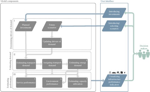
Table 1. Model indicators.

System		Unit
	Demand
Transport	Freight demand	tonne & vehicle
	Passenger demand	passengers & pcu
	Environmental performance
Transport & energy	CO2 emission & energy consumption	tonne & MJ
	System performance
Rail	Railway tracks' freight intensity-capacity ratio	–
	Generalised journey time	hour
Road	Delay factor = Congested travel time/free-flow travel time	–
Waterway	Locks' and waterways' intensity-capacity ratios	–

2.1. Planned investments

Planned investments are current infrastructure planning decisions and cover major sector-specific extension and upgrade investments. These types of investments have long-lasting impacts on capacity and demand changes. For example, the Ministry of Infrastructure and Water Management of the Netherlands publishes the Multi-year Infrastructure, Space and Transport (MIRT) Programme yearly to summarise the planned investments until 2030 (IenW, BZK, and EZK, 2020).

2.2. Core future scenarios

Four distinct future scenarios are adopted from the hybrid disaggregative policy Delphi study of Neef et al. (2020). They span the period until 2050 and are constructed for the context of the Netherlands. The effects of different future behavioural, socioeconomic, environmental, and technological pathways on infrastructure demand and performance can be investigated through these scenarios. Remote working due to the COVID-19 pandemic (Melian and Zebib, 2020) is expected to have a larger impact on transport demand. Scenarios include different levels of fuel mix (i.e. fossil, electricity, and hydrogen) and developments of the load factor, capacity, emission, and energy consumption factors to account for possible technology diffusion and advancements. The narratives of the four scenarios are as follows Neef et al. (2020):

Infraconomy envisions a future in which economic interests act as the main driving force, which results in strong product-based economic developments and the dependency on fossil energy. Liberal market mechanisms favour no energy resource in providing them with tax advantages, while globalisation continues rapidly with increasing global trade. Much will be invested back in expanding infrastructure systems -with more focus on the road- rather than in research and development. In this scenario, limited systematic efforts will be put into tackling the climate crisis. However, some developments, such as the limited modal shift to waterways -proportional to the growth of the port companies- reduce emissions. Face-to-face business meetings are valued more.

Green Revolution represents an environmental-friendly future with noticeable fossil energy utilisation and emission reduction. Policies are directed towards reaching the Paris Agreement's climate goals, with vast investments in the energy transition. This leads to extensive adoption of environmental-friendly technologies and a high societal acceptance of a less polluting lifestyle. Such a lifestyle includes a high level of remote working facilitated by technological developments required for secure and satisfactory distant working. Additionally, polluting energy resources are taxed to encourage a transition towards cleaner resources.

Missed-Boat depicts a future with failed compromises to impose policy measures to tackle the adverse effects of climate change. This future will leave us with different environmental, societal, political, and governance-related challenges, which will cause failure in the attempts to reach a more sustainable society. Environmental-friendly technologies will be adopted to a limited extent. Fossil energy will remain the main energy source, and global trade will be affected by protectionism and political conflicts.

Safety Revolution has broader societal well-being as the central driver. People tend to work less, more meetings will occur virtually, less polluting means of transport will be used, and population growth in rural areas will be higher than in dense urban areas. However, the environmental goals will be achieved less due to slow economic growth. A more conscious lifestyle will result in more local goods consumption. In addition to low economic growth, this trend leads to a reduction in world trade. Furthermore, low research and development budget resulting from low economic growth decreases investments in new technologies and energy transition. Despite the social acceptance of remote working, widespread, reliable, and secure remote working infrastructure will not be available.

The final workshop of the hybrid disaggregative policy Delphi study revealed the Missed-Boat scenario as the most probable future scenario Neef et al. (2020).

2.3. Transport demand sub-models

Environmental, socioeconomic, policy, and technological determinants affect long-term transport demand (Ives et al., 2017). The four future scenarios define directions in which these determinants develop and eventually help estimate infrastructure performance while accounting for future uncertainties. An incremental demand modelling approach forms the basis for the transport demand sub-models, a widely known method for strategic transport planning because of its suitability for communicating model configuration and outcomes, as well as the availability of the required data (de Dios Ortúzar and Willumsen, 2011). These sub-models include sets of endogenous and exogenous variables, which influence trip generations and attractions in the origin-destination (OD) nodes (A and B), as well as the travel costs between origin and destination zones (C) (Lovrić, Blainey, and Preston, 2017). Freight, rail, and road passenger demand sub-models are presented in the following sections.

2.3.1. Road passenger demand

Income, car ownership growth, population size, labour participation, and fuel price are among the major variables defining passenger demand (de Jong and van de Riet, 2008). The considered demand determinants in this model reflect the characteristics of external determinants (e.g. GDP), the influences of the level of service (e.g. travel time), and intermodal competition.

Congestion on a specific corridor will likely affect travel distance and attract travellers from other paths and modes on the corridor (Litman, 2019). Thus, the long-term effect of congested travel time is included in road passenger demand estimation. The induced demand in response to lane extension investments is also considered, in which increased highway capacity attracts new traffic (Hymel, Small, and Van Dender, 2010). Due to added lane kilometres, demand changes arise from the shifts in trip time, route, mode, and further car use. Since train ticket price changes contribute inversely to the road demand change and play an important role in the mode switch, they are included in the model.

Moreover, railway travel time and convenience affect mode shifts between road and railway networks, which is considered by the railway generalised journey time (GJT) in road passenger demand estimation -explained in Section 2.3.2. The road demand estimation formulation (Equation (1(1) $\begin{array}{rll}{D}_{ijt}& =D_{ijt-1}{\left(\frac{J_{it}^{\mathrm{\prime }}}{J_{it-1}^{\mathrm{\prime }}}\right)}^{{\eta }_J}{\left(\frac{P_{it}}{P_{it-1}}\right)}^{{\eta }_P}{\left(\frac{J_{jt}^{\mathrm{\prime }}}{{J^{\mathrm{\prime }}}_{jt-1}}\right)}^{{\eta }_J}{\left(\frac{P_{jt}}{P_{jt-1}}\right)}^{{\eta }_P}& \\ & {\left(\frac{E_{ijt}}{E_{ijt-1}}\right)}^{{\eta }_E}{\left(\frac{F_t}{F_{t-1}}\right)}^{{\eta }_F}{\left(\frac{G_t}{G_{t-1}}\right)}^{{\eta }_G}{\left(\frac{GJ{T}_{ijt}}{GJ{T}_{ijt-1}}\right)}^{{\eta }_{GJT}}\\ & {\left(\frac{T{T}_{ijt}^{road}}{T{T}_{ijt-1}^{road}}\right)}^{{\eta }_{T{T}^{road}}}{\left(\frac{TT{P}_t}{TT{P}_{t-1}}\right)}^{{\eta }_{TTP}}{\left(\frac{V_t}{V_{t-1}}\right)}^{{\eta }_V}\end{array}$(1) )) covers the most current elasticity values relevant in the Dutch context. These values are based on literature and policy documents from the Netherlands -Table 2. They are represented by a column vector $\eta =[{\eta }_J,{\eta }_P,{\eta }_J,{\eta }_F,{\eta }_G,{\eta }_{TP},{\eta }_V,{\eta }_E,{\eta }_{T{T}^{road}}{]}^{⊺}$. (1) $\begin{array}{rll}{D}_{ijt}& =D_{ijt-1}{\left(\frac{J_{it}^{\mathrm{\prime }}}{J_{it-1}^{\mathrm{\prime }}}\right)}^{{\eta }_J}{\left(\frac{P_{it}}{P_{it-1}}\right)}^{{\eta }_P}{\left(\frac{J_{jt}^{\mathrm{\prime }}}{{J^{\mathrm{\prime }}}_{jt-1}}\right)}^{{\eta }_J}{\left(\frac{P_{jt}}{P_{jt-1}}\right)}^{{\eta }_P}& \\ & {\left(\frac{E_{ijt}}{E_{ijt-1}}\right)}^{{\eta }_E}{\left(\frac{F_t}{F_{t-1}}\right)}^{{\eta }_F}{\left(\frac{G_t}{G_{t-1}}\right)}^{{\eta }_G}{\left(\frac{GJ{T}_{ijt}}{GJ{T}_{ijt-1}}\right)}^{{\eta }_{GJT}}\\ & {\left(\frac{T{T}_{ijt}^{road}}{T{T}_{ijt-1}^{road}}\right)}^{{\eta }_{T{T}^{road}}}{\left(\frac{TT{P}_t}{TT{P}_{t-1}}\right)}^{{\eta }_{TTP}}{\left(\frac{V_t}{V_{t-1}}\right)}^{{\eta }_V}\end{array}$(1) (2) ${J^{\mathrm{\prime }}}_t=\left(\frac{W{D}_t-RW{D}_t\cdot PR{W}_t}{W{D}_t}\right)J_t$(2)

• η: Elasticity values, (see Table 2)

• $D_{ijt}$: Number of trips between zones i to j at time t

• E: Road lane-kilometer extension

• F: Fuel price

• G: GDP

• GJT: Railway generalised journey time

• J: Number of jobs

• $J^{\mathrm{\prime }}$: Number of commuting jobs

• P: Population

• $T{T}^{road}$: Road congested travel time

• TTP: Train ticket price

• V: Number of vehicles

• RWD: Average remote working days

• WD: Average working days

• PRW: Percentage of the remote workers

Table 2. Elasticity values of the determinants of road passenger demand.

Parameter	Value	Reference
${\eta }_E$	0.25	van der Loop et al. (2016)
${\eta }_F$	−0.17	Groot and van Mourik (2012)
${\eta }_G$	0.38	van Dender and Clever (2013)
${\eta }_{GJT}$	0.14	Wardman et al. (2018)
${\eta }_J$	0.64	van der Loop (2018)
${\eta }_P$	0.33	van der Loop (2018)
${\eta }_{TTP}$	0.02	Geilenkirchen et al. (2010)
${\eta }_{T{T}^{road}}$	−1.1	van der Loop et al. (2016)
${\eta }_V$	0.6	van der Loop (2018)

2.3.2. Railway passenger demand

Railway passenger demand is estimated based on a wide range of demand determinants (Equation (3(3) $\begin{array}{rll}\eta & =[{\eta }_F,{\eta }_{GJT},{\eta }_I,{\eta }_J,{\eta }_P,{\eta }_{TP},{\eta }_{TTP},{\eta }_{T{T}^{road}},{\eta }_V{]}^{⊺}.& \\ D_{ijt}& =D_{ijt-1}{\left(\frac{J_{it}^{\mathrm{\prime }}}{J_{it-1}^{\mathrm{\prime }}}\right)}^{{\eta }_J}{\left(\frac{P_{it}}{P_{it-1}}\right)}^{{\eta }_P}{\left(\frac{J_{jt}^{\mathrm{\prime }}}{J_{jt-1}^{\mathrm{\prime }}}\right)}^{{\eta }_J}{\left(\frac{P_{jt}}{P_{jt-1}}\right)}^{{\eta }_P}\\ & {\left(\frac{F_t}{F_{t-1}}\right)}^{{\eta }_F}{\left(\frac{GJ{T}_{ijt}}{GJ{T}_{ijt-1}}\right)}^{{\eta }_{GJT}}{\left(\frac{I_t}{I_{t-1}}\right)}^{{\eta }_I}{\left(\frac{T{P}_{ijt}}{T{P}_{ijt-1}}\right)}^{{\eta }_{TP}}\\ & {\left(\frac{T{T}_{ijt}^{road}}{T{T}_{ijt-1}^{road}}\right)}^{{\eta }_{T{T}^{road}}}{\left(\frac{TT{P}_t}{TT{P}_{t-1}}\right)}^{{\eta }_{TTP}}{\left(\frac{V_t}{V_{t-1}}\right)}^{{\eta }_V}\end{array}$(3) )), including socioeconomic characteristics of public transport (e.g. travel time, cost, service level, and comfort), as well as features of other modes affecting railway passenger demand such as travel time on the road network and vehicle ownership (van der Loop et al. “Explaining the Development” , 2018). The train crowdedness between each origin-destination (OD) pair affects trip comfort and, thus, passenger demand. This phenomenon is considered through the generalised journey time (GJT, Equation (4(4) $GJ{T}_{ijt}=w_{Lt}\times T_{ijt}+P_{ijt}$(4) )). The mentioned variables play a significant role in the mode shift and competition. Table 3 presents the elasticity values of the demand determinants, which are derived based on literature and policy documents from the Netherlands. A column vector represents them: (3) $\begin{array}{rll}\eta & =[{\eta }_F,{\eta }_{GJT},{\eta }_I,{\eta }_J,{\eta }_P,{\eta }_{TP},{\eta }_{TTP},{\eta }_{T{T}^{road}},{\eta }_V{]}^{⊺}.& \\ D_{ijt}& =D_{ijt-1}{\left(\frac{J_{it}^{\mathrm{\prime }}}{J_{it-1}^{\mathrm{\prime }}}\right)}^{{\eta }_J}{\left(\frac{P_{it}}{P_{it-1}}\right)}^{{\eta }_P}{\left(\frac{J_{jt}^{\mathrm{\prime }}}{J_{jt-1}^{\mathrm{\prime }}}\right)}^{{\eta }_J}{\left(\frac{P_{jt}}{P_{jt-1}}\right)}^{{\eta }_P}\\ & {\left(\frac{F_t}{F_{t-1}}\right)}^{{\eta }_F}{\left(\frac{GJ{T}_{ijt}}{GJ{T}_{ijt-1}}\right)}^{{\eta }_{GJT}}{\left(\frac{I_t}{I_{t-1}}\right)}^{{\eta }_I}{\left(\frac{T{P}_{ijt}}{T{P}_{ijt-1}}\right)}^{{\eta }_{TP}}\\ & {\left(\frac{T{T}_{ijt}^{road}}{T{T}_{ijt-1}^{road}}\right)}^{{\eta }_{T{T}^{road}}}{\left(\frac{TT{P}_t}{TT{P}_{t-1}}\right)}^{{\eta }_{TTP}}{\left(\frac{V_t}{V_{t-1}}\right)}^{{\eta }_V}\end{array}$(3) (4) $GJ{T}_{ijt}=w_{Lt}\times T_{ijt}+P_{ijt}$(4)

• η: Elasticity values, (see Table 3)

• I: Income

• TP: Train punctuality

Table 3. Elasticity values of the determinants of railway transport demand.

Parameter	Value	Reference
${\eta }_F$	0.11	KiM (2019)
${\eta }_{GJT}$	−1.51	van der Loop et al. “Verklaring van de ontwikkeling” (2018)
${\eta }_I$	0.27	KiM (2019)
${\eta }_J$	0.29	KiM (2019)
${\eta }_P$	1.38	KiM (2019)
${\eta }_{TP}$	1.1	MuConsult (2015)
${\eta }_{TTP}$	−0.63	KiM (2019)
${\eta }_{T{T}^{road}}$	0.24	van der Loop et al. (2016)
${\eta }_V$	−0.02	KiM (2019)

In Equation (4(4) $GJ{T}_{ijt}=w_{Lt}\times T_{ijt}+P_{ijt}$(4) ), GJT is the generalised journey travel time between OD pairs, which depends on the journey time, equivalent time penalties ($P_{ijt}$, representing headway and the need to change trains), and the trip crowdedness, which refers to the number of passengers in each train (Wardman and Murphy, 2015). Time penalties translate headway into journey time by a weighting factor of 1.5 for the Netherlands (Zwaneveld et al., 2009). T is the journey time between OD pairs, and $w_L$ is the multiplier representing the crowdedness in terms of the journey time. Here a time-based valuation is used as it is more transferable across contexts and countries compared to monetary valuation (Wardman and Whelan, 2011). We base $w_L$ on the multipliers derived from a meta-analysis of 15 empirical studies in Wardman and Whelan (2011), quantifying the variation of the crowdedness multiplier against different load factors (LF) -representing crowdedness (Table 4). We modified the multipliers by making a weighted average of seated and standing multipliers. Weights are defined based on the seated and standing passengers ratio for each load factor.

Table 4. w_L multipliers for each load factor.

LF(%)	wL
50	0.95
75	1.05
100	1.40
125	1.59
150	1.79
175	2.01
200	2.26

2.3.3. Freight transport demand

Economic and world trade developments are among the most influential demand determinants for freight demand (Knoope and Francke, 2020, van de Riet, Jong, and Walker, 2004). In this model, the long-term effects of GDP change and the share of the service industry in GDP are addressed to account for economic activities and the switch towards service and knowledge industries, respectively. The world trade index represents globalisation, affecting the international freight demand (Kupfer et al., 2017). We have included the effects of travel time and fuel prices on freight demand, which allows us to address transport costs.

Travel time and fuel prices can trace the effects of competition between transport modes. Fuel prices also indicate the dependency on the energy sector. However, travel time and fuel price effects have a limited impact on freight demand compared to the other determinants (Knoope and Francke, 2020, KiM, 2017). Fuel prices have a negative effect on road transport while affecting railway and waterway networks positively. That is because road transport reacts quicker to fuel price fluctuations and is more influential in defining demand. Equation (5(5) $\begin{array}{rll}\eta & =[{\eta }_F,{\eta }_G,{\eta }_{GS},{\eta }_{T{T}^n},{\eta }_W{]}^{⊺}.& \\ D_{ijt}^m& =D_{ijt-1}^m{({\alpha }_{ij}+{\omega }_{ij}\frac{G_t}{G_{t-1}})}^{{\eta }_G}{\left(\frac{G{S}_t}{G{S}_{t-1}}\right)}^{{\eta }_{GS}}{\left(\frac{F_t^m}{F_{t-1}^m}\right)}^{{\eta }_{F^m}}\\ & \prod _{n\in M}{\left(\frac{T{T}_{ijt}^n}{T{T}_{ijt-1}^n}\right)}^{{\eta }_{T{T}^{mn}}}{({\omega }_{ij}+{\alpha }_{ij}\frac{W_t}{W_{t-1}})}^{{\eta }_W}\end{array}$(5) ) estimates the freight road demand for mode $m\in M$ -a set that includes all modes- using the railway, road, and waterway networks. Table 5 presents the elasticity values of the demand determinants, which are derived based on literature and policy documents from the Netherlands. A column vector represents them: (5) $\begin{array}{rll}\eta & =[{\eta }_F,{\eta }_G,{\eta }_{GS},{\eta }_{T{T}^n},{\eta }_W{]}^{⊺}.& \\ D_{ijt}^m& =D_{ijt-1}^m{({\alpha }_{ij}+{\omega }_{ij}\frac{G_t}{G_{t-1}})}^{{\eta }_G}{\left(\frac{G{S}_t}{G{S}_{t-1}}\right)}^{{\eta }_{GS}}{\left(\frac{F_t^m}{F_{t-1}^m}\right)}^{{\eta }_{F^m}}\\ & \prod _{n\in M}{\left(\frac{T{T}_{ijt}^n}{T{T}_{ijt-1}^n}\right)}^{{\eta }_{T{T}^{mn}}}{({\omega }_{ij}+{\alpha }_{ij}\frac{W_t}{W_{t-1}})}^{{\eta }_W}\end{array}$(5) (6) $\begin{array}{rl}{\alpha }_{ij}& =\{\begin{array}{ll}0,\mathrm{i}\mathrm{f}i\mathrm{a}\mathrm{n}\mathrm{d}j\mathrm{a}\mathrm{r}\mathrm{e}\mathrm{o}\mathrm{n}\mathrm{a}\mathrm{d}\mathrm{o}\mathrm{m}\mathrm{e}\mathrm{s}\mathrm{t}\mathrm{i}\mathrm{c}\mathrm{f}\mathrm{r}\mathrm{e}\mathrm{i}\mathrm{g}\mathrm{h}\mathrm{t}\mathrm{r}\mathrm{o}\mathrm{u}\mathrm{t}\mathrm{e}& \\ 1,\mathrm{i}\mathrm{f}i\mathrm{a}\mathrm{n}\mathrm{d}j\mathrm{a}\mathrm{r}\mathrm{e}\mathrm{o}\mathrm{n}\mathrm{a}\mathrm{n}\mathrm{i}\mathrm{n}\mathrm{t}\mathrm{e}\mathrm{r}\mathrm{n}\mathrm{a}\mathrm{t}\mathrm{i}\mathrm{o}\mathrm{n}\mathrm{a}\mathrm{l}\mathrm{f}\mathrm{r}\mathrm{e}\mathrm{i}\mathrm{g}\mathrm{h}\mathrm{t}\mathrm{r}\mathrm{o}\mathrm{u}\mathrm{t}\mathrm{e}\end{array}\end{array}$(6) (7) $\begin{array}{rl}{\omega }_{ij}& =\{\begin{array}{ll}1,\mathrm{i}\mathrm{f}i\mathrm{a}\mathrm{n}\mathrm{d}j\mathrm{a}\mathrm{r}\mathrm{e}\mathrm{o}\mathrm{n}\mathrm{a}\mathrm{d}\mathrm{o}\mathrm{m}\mathrm{e}\mathrm{s}\mathrm{t}\mathrm{i}\mathrm{c}\mathrm{f}\mathrm{r}\mathrm{e}\mathrm{i}\mathrm{g}\mathrm{h}\mathrm{t}\mathrm{r}\mathrm{o}\mathrm{u}\mathrm{t}\mathrm{e}& \\ 0,\mathrm{i}\mathrm{f}i\mathrm{a}\mathrm{n}\mathrm{d}j\mathrm{a}\mathrm{r}\mathrm{e}\mathrm{o}\mathrm{n}\mathrm{a}\mathrm{i}\mathrm{n}\mathrm{t}\mathrm{e}\mathrm{r}\mathrm{n}\mathrm{a}\mathrm{t}\mathrm{i}\mathrm{o}\mathrm{n}\mathrm{a}\mathrm{l}\mathrm{f}\mathrm{r}\mathrm{e}\mathrm{i}\mathrm{g}\mathrm{h}\mathrm{t}\mathrm{r}\mathrm{o}\mathrm{u}\mathrm{t}\mathrm{e}\end{array}\end{array}$(7)

• GS: Share of the service sector in GDP

• W: World trade

Table 5. Elasticity values of the determinants of freight transport demand.

Parameter	Mode	Value	Reference
${\eta }_G$	Rail, Road, Waterway		0.57		KiM (2019)
${\eta }_{GS}$	Rail, Road, Waterway		−0.8		KiM (2019)
${\eta }_W$	Rail, Road, Waterway		0.41		KiM (2019)
${\eta }_F$	Rail		0.22		Geilenkirchen et al. (2010)
	Road		−0.07		Geilenkirchen et al. (2010)
	Waterway		0.06		Geilenkirchen et al. (2010)
		Railway	Road	Waterway
1l${\eta }_{TT}$	Rail	−0.211	0.223	0.6	De Jong et al. (2011)
	Road	–	−0.1	0.086	De Jong et al. (2011)
	Waterway	–	0.231	−0.284	De Jong et al. (2011)

2.4. Infrastructure performance sub-models

In addition to passenger and freight demand sub-models, we introduce sub-models for measuring infrastructure performance. We consider environmental and system performance indicators in two categories of performance sub-models (Table 1).

2.4.1. System performance indicators

After estimating transport demand, traffic assignment sub-models distribute the demand on the networks of all modalities and estimate the link travel times and the amount of traffic on each network link. These outputs are then used to reflect the performance developments of the systems. Moreover, the updated link travel times based on the traffic congestion levels are fed back into the demand estimation model, as travel time is one of the transport demand determinants. These two steps are taken iteratively until the demand changes remain within an acceptable range or a maximum number of times. To control the differences between each iteration, absolute and relative tolerances of ${10}^{-6}$ and ${10}^{-3}$ are chosen.

2.4.1.1 Railway network

The generalised journey time (GJT) represents the railway performance state, which depends on train frequencies and crowdedness. In order to determine the GJT, the crowdedness along different railway tracks should be determined. The demands of OD pairs are assigned to the routes with the shortest travel time and are based on the existing timetables and train frequencies of routes. Furthermore, the intensity-capacity ratio is calculated for all railway tracks to show the capacity utilisation of railway tracks for freight transport.

2.4.1.2 Road network

Delay factor represents the ratio between the congested travel time and the free-flow travel time in traffic situations with no congestion. A capacity restraint traffic assignment based on the Bureau of Public Roads (BPR) method is implemented. This method offers a popular volume-delay function (VDF, see Equation (8(8) $T=T_{ff}(1+0.64{\left(\frac{q}{q_{pc}}\right)}^4)$(8) )) to be used in strategic transport planning (Bliemer et al., 2017) due to its simple mathematical form and the limited input requirements (Maerivoet and Moor, 2005, Mtoi and Moses, 2014). Asgarpour et al. (2023) calibrated the VDF using 995 measurement points for multiple lane road links, with a root mean square error of (RMSE) of 7.39 -without outliers, the RMSE yields 3.27. As this paper focuses on implementing the proposed system-of-systems model in the context of the Netherlands, this calibrated VDF is used. (8) $T=T_{ff}(1+0.64{\left(\frac{q}{q_{pc}}\right)}^4)$(8)

• q: traffic flow

• $q_{pc}$: Road segment practical capacity

• T: Congested travel time

• $T{T}_{ff}$: Free-flow travel time

• The bi-conjugate Frank-Wolfe (BFW) algorithm is used, which performs more efficiently compared to other converging link-based traffic assignment algorithms (Mitradjieva and Olov Lindberg, 2013). For this purpose, we used AequilibraE, an open-source and comprehensive Python package for transportation modelling. The AequilibraE open-source and comprehensive Python package is used for the assignment (Camargo, Zill, and O'Brien, 2018).

2.4.1.3 Waterway network

The intensity-capacity ratio (I/C) is used to measure the waterway network performance. Numerous interconnected factors at different levels affect vessel distributions in waterway networks. These included factors related to the waterway and intersection characteristics, vessel type and dimensions, navigation, weather conditions, sailing rules, and behaviour (Bellsolà Olba et al., 2019, 2015). This paper simplifies the route choice decision to travel time minimisation. Similar to the road network assignment, the BFW algorithm is used to converge to the Wardrop equilibrium.

Travel time represents the free-flow travel time along the waterways, the service times for moveable bridges, and the total lock transit time (cycles and waiting). Maximum speed for each waterway link is derived by considering the type of sailing vessels, the waterway CEMT class, load, water flow direction, and speed (BIVAS, 2018). The service times of moveable bridges are specific to each and have a static value. The total lock transit time depends on the lock capacity (c) and the intensity (I) of the passing traffic (Bückmann et al., 2009).

The I/C can express the average transit time. Table 6 shows the relationship according to the yearly waterway guideline published by Rijkswatertaat, the executive branch of the Ministry of Infrastructures of the Netherlands (Koedijk, 2020). The total lock transit time is approximated as a continuous function of the intensity to capacity ratio, using Table 6. The capacity of each lock is separately calculated. Waiting time in terminals and ports is not considered in this study.

Table 6. Lock transit time based on lock I/C.

I/C ratio	verage transit time (min.)
0.3	25
0.4	30
0.5	45
0.6	60
0.7	80
0.8	125
0.9	235

2.4.2. Environmental performance indicators

Transportation is one of the main sources of CO₂, which contributes to climate change, imposes health risks, and adversely affects nature and biodiversity. Equations (9(9) $\begin{array}{rll}E{C}_{ij}^m& =L_{ij}(\sum _{e\in E_F^m}\sum _{v\in V_F^m}EC{F}_F^{mev}\cdot F_{Fij}^m\cdot S_F^v\cdot E{M}_F^{me}& \\ & +\sum _{e\in E_P^m}\sum _{v\in V_P^m}EC{F}_P^{mev}\cdot F_{Pij}^m\cdot S_P^v\cdot E{M}_P^{me})\end{array}$(9) ) and (10(10) $\begin{array}{rll}C{E}_{ij}^m& =L_{ij}(\sum _{e\in E_F^m}\sum _{v\in V_F^m}CE{F}_F^{mev}\cdot F_{Fij}^m\cdot S_F^v\cdot E{M}_F^{me}& \\ & +\sum _{e\in E_P^m}\sum _{v\in V_P^m}CE{F}_P^{mev}\cdot F_{Pij}^m\cdot S_P^v\cdot E{M}_P^{me})\end{array}$(10) ) calculate the transport energy consumption and emission bottom-up using variable flows, emission, and energy consumption factors.

In Equation (9(9) $\begin{array}{rll}E{C}_{ij}^m& =L_{ij}(\sum _{e\in E_F^m}\sum _{v\in V_F^m}EC{F}_F^{mev}\cdot F_{Fij}^m\cdot S_F^v\cdot E{M}_F^{me}& \\ & +\sum _{e\in E_P^m}\sum _{v\in V_P^m}EC{F}_P^{mev}\cdot F_{Pij}^m\cdot S_P^v\cdot E{M}_P^{me})\end{array}$(9) ), $E{C}_{ij}^m$ is the energy consumption of the mode m between i and j (MJ); $L_{ij}$ is the segment length between i and j (km); $EC{F}_F^{mev}$ and $EC{F}_P^{mev}$ represent the energy consumption factor of the vehicle v powered by the energy resource e within the mode m for freight and passenger transport. $F_F^m$ and $F_P^m$ are the modes m freight flow between i and j (tonne) and passenger flow (number of vehicles for roads and railways, respectively). $V_F^m$ and $V_P^m$ are the sets of representative vehicles and vessels used in mode m to transport freight and passenger. $E_F^m$ and $E_P^m$ are the sets of energy resources consumed in mode m. $S_F^v$ and $S_P^v$ are the share of the vehicle or vessel used to transport freight or passenger in mode m (Kuiper and Ligterink, 2013, CE Delft, 2015, 2020). $E{M}_F^{me}$ and $E{M}_P^{me}$ are the energy mix share of the energy resource e for the freight and passenger transport of the mode m.

In Equation (10(10) $\begin{array}{rll}C{E}_{ij}^m& =L_{ij}(\sum _{e\in E_F^m}\sum _{v\in V_F^m}CE{F}_F^{mev}\cdot F_{Fij}^m\cdot S_F^v\cdot E{M}_F^{me}& \\ & +\sum _{e\in E_P^m}\sum _{v\in V_P^m}CE{F}_P^{mev}\cdot F_{Pij}^m\cdot S_P^v\cdot E{M}_P^{me})\end{array}$(10) ), $C{E}_{ij}^m$ is Well-to-Wheel CO₂ emission between i and j for mode m (tonne); $CE{F}_F^{mev}$ and $CE{F}_P^{mev}$ are CO₂ emission factor of the vehicle v of the mode m for freight and passenger transport (g/tkm, g/vkm). We distinguished between two passenger train types, sprinters and intercity trains, which differ in weight, number of seats, number of stops, and frequencies. Such differences result in different energy consumption and emissions. (9) $\begin{array}{rll}E{C}_{ij}^m& =L_{ij}(\sum _{e\in E_F^m}\sum _{v\in V_F^m}EC{F}_F^{mev}\cdot F_{Fij}^m\cdot S_F^v\cdot E{M}_F^{me}& \\ & +\sum _{e\in E_P^m}\sum _{v\in V_P^m}EC{F}_P^{mev}\cdot F_{Pij}^m\cdot S_P^v\cdot E{M}_P^{me})\end{array}$(9) (10) $\begin{array}{rll}C{E}_{ij}^m& =L_{ij}(\sum _{e\in E_F^m}\sum _{v\in V_F^m}CE{F}_F^{mev}\cdot F_{Fij}^m\cdot S_F^v\cdot E{M}_F^{me}& \\ & +\sum _{e\in E_P^m}\sum _{v\in V_P^m}CE{F}_P^{mev}\cdot F_{Pij}^m\cdot S_P^v\cdot E{M}_P^{me})\end{array}$(10)

3. Case study

3.1. Region

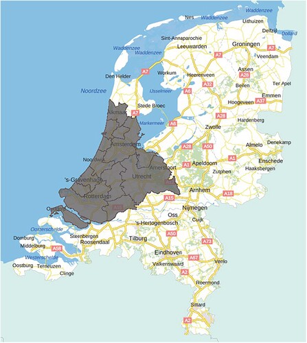
The case study region (Figure 2) covers the three most populated Dutch provinces of Noord-Holland, Zuid-Holland, and Utrecht. This region also includes the two biggest ports of the Netherlands (Rotterdam and Amsterdam), which adds to the region's national and international economic importance. Two major European railway routes (Trans-European Network for Transport), a part of the Betuweroute, and major waterways, such as Hollandse Diep and Amsterdam-Rijnkanaal, cross the region. The economic and social importance of the area makes it a suitable case to implement the proposed model and generate insights relevant to policymakers and infrastructure agencies. In the case study region, nearly all railway tracks are electrified and run on electricity (PBL, CBS, TNO, and RIVM, 2020).

Figure 2. Case study region.

Municipalities represent the finest spatial aggregation level. Road infrastructure consists of the main highways (A-roads) and national roads (N-roads). Railway infrastructure covers railway stations and tracks. Waterways with CEMT class above III are also included. Sets of nodes and links represent the transport systems. In order to avoid possible distortions in gathered data due to the COVID-19 pandemic in 2020 and 2021, 2019 is set as the base year. The simulation time horizon is 2050 with a one-year time step. Extended evening peak hours from 16:00 till 20:00 are selected to estimate demand because this period has the most congestion, mainly because of the overlapping work-home and leisure trips (Hilbers et al., 2020).

3.2. Data

Three categories of infrastructure attributes, performance, and spatial data are collected. Spatial data contain the location and dimensions of infrastructure. The infrastructure attribute data (e.g. capacity and maximum allowed speed) include necessary inputs to estimate infrastructure demand and performance. Open-source national databases and data sets acquired by the infrastructure owners (Port of Rotterdam, ProRail, Rijkswaterstaat) and Statistics Netherlands (CBS) are the major data sources (NDW, 2020, Rijksoverheid, 2020, PDOK, 2020). QGIS processing algorithms and python scripts process the data used in the demand and performance estimation sub-models. The processing tasks aggregate the data instances to a suitable spatial resolution, check the connectivity, derive the base year demand and performance, derive the transport demand nodes, join infrastructure and performance attributes to spatial data sets, and simplify the data set instances.

3.3. Base year OD matrices

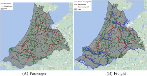
OD matrices at the base year are required to estimate the demand developments. Freight OD matrices are created based on the CSV data received from Statistics Netherlands (CBS), which are processed and mapped uniformly from NUTS3 -the finest aggregation level according to the received data- to the demand nodes of each network. The international origins and destinations include the major freight transport corridors towards Austria, Belgium, Denmark, Spain, France, Italy, Poland, and Sweden. The Railway passenger OD matrix among stations is derived based on passenger stream data received from the railway infrastructure agency (ProRail). The used passenger OD matrices are based on the estimated OD matrices by Asgarpour et al. (2023). Figure 3 presents the included transport networks and zones.

Figure 3. Transport networks and zones. (a) Passenger. (b) Freight.

3.4. Planned investments

Four planned investments in railway, road, port, and waterway networks are considered. For the railway network, train frequency-increasing investments are introduced to the presented model based on the high-frequency trajectory programme of the infrastructure ministry (IenW, 2020). This includes trajectories from and to the major cities within the case study region, such as Amsterdam, The Hague, Rotterdam, and Utrecht. Road network investments match the planned investments of the multi-year programme for infrastructure, space, and transport (MIRT) within the case study region, which include both new constructions (in 2023 and 2024) and extensions (parts of A1, A4, A6, A9, A10, A12, A20, and A28 highways planned for 2026, 2027, 2028, 2030, and 2036) (IenW, BZK, and EZK, 2020).

The model contains a port investment, which increases the capacity of Prinses Amaliahaven by 28% within 2 phases (Port of Rotterdam, 2021). In order to be able to trace the effect of such an investment with the presented model, we assume an elasticity of 1. This means that a 10% capacity increase results in a 10% demand increase for that specific port, represented by a node in the sets of waterway nodes and links. Such a demand increase occurs within three years to account for a gradual demand increase resulting from a major investment.

A major waterway investment is the lock capacity increase of the Volkeraksluizen IenW, BZK, and EZK (2020). This is one of the major lock complexes situated on the southern boundary of the case study region. The capacity increase affects the capacity of the waterway links connected to the lock complex, which in turn affects the transport time, demand assignment, and demand estimation for the southern freight corridor.

3.5. Future scenarios

Table 7 summarises the core scenarios described in Section 2.2. The four core scenarios (Infraconomy, Safety Revolution, Missed Boat, and Green Revolution) were adapted to provide the sub-models (Section 2.3) with quantified input variables. Asgarpour et al. (2023) systematically extended the presented core scenarios by implementing the Shared Socioeconomic Pathway (SSP) framework and using scenarios developed by the Dutch Environmental Assessment Agency (WLO scenarios) (Manders and Joannes Maria Kool, 2015). GDP, number of vehicles, and the world trade projections are updated in this research based on the most recent WLO scenario calibrations to reflect possible future developments (IenW, 2021a, 2021b). Table 8 demonstrates the development of the demand determinants and modelling parameters for each scenario in 2030 and 2050.

Table 7. Scenario description.

	State change direction and extent compared to the base year
Scenario's aspect	Infraconomy	Green revolution	Missed boat	Safety revolution
Main drivers	Increases in infrastructure length lead to increases in economic development	Maximise climate and environmental-friendly development	Making compromises between environment, infrastructure and economy and individualism	Well-being is more important than welfare, especially expressed in safety and reliability
Investments in innovation	Moderate increase	High increase	Low increase	Low increase
Economic development	High increase;	High increase;	Low increase;	Low increase;
	Business climate is enhanced (nationally and internationally)	Green transition is an ex-port product	National competitive position cannot be maintained	Shorter work week, less money being ‘pumped around’
Environment protection	No change;	Very high increase;	Low decrease;	Moderate decrease;
commitment	Environment protection is not considered in policy, and societal goal setting	Major green-minded commitment	Compromised goal-setting with an insufficient and volatile political and societal commitment to reach sustainable goals	Insufficient money to effectively develop technologies to combat pollution
Mobility behaviour	Very high inclination to travel;	Moderate inclination to travel;	High inclination to travel;	High inclination to not travel;
	Favoring face-to-face contacts	A major shift away from road and aviation to rail	Reduced aviation, shift to other modes	Minimising travel
Transport energy mix	Moderate increase;	High decrease;	Moderate decrease;	Moderate decrease;
	Consists of both fossil and green sources, fossil fuels remain the primary resource as they keep their economic advantages	Replacing fossil energy usage with high and efficient usage of renewable energy	Decrease of fossil sources in favor of renewable to increase wellbeing -- overall limited willingness to decrease usage	Decrease of fossil sources in favor of renewable to increase wellbeing -- overall willingness to decrease usage

Table 8. Emission, energy, and transport demand input variables for each future scenario.

	Values for 2030 and 2050
Input variables (index 100 at 2019)	Infraconomy revolution	Safety revolution	Missed boat	Green revolution	Energy resource	Infrastructure
Average remote working days (days/week)	1.65, 1.8	2, 2.5	1.7, 2	2, 3	n.a.	All
Average working days (days/week)	4.375, 4.625	4.25, 3.75	4.375, 4.75	4.375, 4.375	n.a.	All
Electricity excise duty to electricity price (%)	1.4, 1.4	1.4, 1.4	1.4, 1.4	1.25, 0.8	n.a.	All
Fossil fuel excise duty to fuel price (%)	2, 2	2, 2	2, 2	3, 5	n.a.	All
Fossil fuel price (US2013$/barrel)	100, 120	67, 80	138, 162	67, 80	n.a.	All
GDP (index)	130, 180	110, 120	110, 120	120, 150	n.a.	All
Income (index)	120, 285	110, 210	110, 210	115, 240	n.a.	All
Jobs (mil.)	11.8, 12.3	10.8, 10.4	10.8, 10.4	11.8, 12.3	n.a.	All
Load capacity (index)	110, 130	105, 115	105, 115	115, 145	All	Road & Waterway
Load factor (%)	0.46, 0.52	0.44, 0.48	0.44, 0.48	0.49, 0.62	All	Road
	0.57, 0.64	0.56, 0.60	0.56, 0.60	0.60, 0.75	All	Waterway
Percentage of the remote workers(%)	35,40	40,50	38,42	45,60	n.a.	All
Population (mil.)	18.2, 18.5	17.7, 17	18.7, 19.9	17.7, 17	n.a.	All
Share of the service sector in GDP (%)	77, 81	75.5, 79	74, 77	77, 81	n.a.	All
Train punctuality (index)	96, 88	102, 105	101, 102	100, 101	n.a.	Rail
Train ticket price (index)	103, 105	102, 103	102, 104	102, 103	n.a.	Rail
Vehicles (mil.)	9.9, 11.6	8.9, 9.4	9.4, 10.5	9.4, 10.5	n.a.	Road
Vehicle capacity (passengers)	320, 410	305, 345	305, 345	335, 470	n.a.	Rail
World trade (index)	160, 380	140, 250	140, 250	150, 320	n.a.	All
$CE{F}_F$ (index)	79, 57	75, 49	75, 49	74, 48	Diesel	All
	99, 97	82, 64	82, 64	49, 15	Electricity	All
	89, 77	75, 51	75, 51	70, 40	H2	All
$CE{F}_P$ (index)	83, 65	77, 53	77, 53	78, 56	Petrol	Road
	99, 97	82, 64	82, 64	49, 15	Electricity	All
	89, 77	75, 51	75, 51	70, 40	H2	All
$EC{F}_F$ (index)	92, 83	88, 75	88, 75	85, 69	Diesel	All
	97, 93	90, 80	90, 80	85, 60	Electricity	All
	100, 100	100, 100	100, 100	98, 95	H2	All
$EC{F}_P$ (index)	79, 58	75, 50	75, 50	77, 53	Petrol	Road
	97, 93	90, 80	90, 80	85, 60	Electricity	All
	100, 100	100, 100	100, 100	98, 95	H2	All
Freight energy mix (%)	10, 0	0, 0	5, 0	0, 0	Diesel	Rail
	90, 95	100, 85	95, 90	95, 70	Electricity	Rail
	0, 5	0, 15	0, 10	5, 30	H2	Rail
	95, 88	88, 73	91, 82	71, 27	Diesel	Road
	5, 12	12, 26	9, 18	29, 71	Electricity	Road
	0, 0	0, 0	0, 0	0, 2	H2	Road
	90, 75	80, 55	85, 60	70, 20	Diesel	Waterway
	10, 25	20, 35	15, 35	25, 60	Electricity	Waterway
	0, 0	0, 10	0, 5	5, 20	H2	Waterway
Passenger energy mix (%)	100, 95	100, 85	100, 90	95, 70	Electricity	Rail
	0, 5	0, 15	0, 10	5, 30	H2	Rail
	7, 14	14, 28	11, 20	30, 73	Electricity	Road
	0, 1	0, 1	0, 1	0, 1	H2	Road
	93, 85	86, 70	89, 79	69, 23	Petrol	Road

3.5.1. Consumer and representative energy prices

This model includes different fuel and energy price levels and estimates the possible effects of these levels on transport demand. Fuel price elasticity is considered because it is the only energy resource-related price-demand elasticity in the context of the Netherlands. Fuel elasticity remains constant in this model, while the sensitivity of the transport demand to the fuel price depends on the fuel mix -with electricity and fossil having the major shares. We define the representative energy price and use it to trace the effect on transport demand considering the energy mix in each scenario. The representative energy price is the weighted sum of electricity and fossil fuel consumer price (per kWh). Weights are derived based on the share of the energy resource in the mix in each simulation time step. Consumer electricity and fossil fuel prices are based on the oil barrel prices, fossil fuel and electricity excise duty, and the share of the excise duty values in the consumer prices for energy resources. Asgarpour et al. (2023) have elaborated on determining the consumer energy prices for road users, according to which we defined the scenario projections.

3.5.2. Emission and energy efficiency factors

CE Delft (2015) found a share of 25% for short-distance trains (sprinters) and 75% for intercity trains. For the freight trains and in the base year -based on the research done by CE Delft (2020)- we assume a share of 65% for electric and 35% for the diesel-driven trains -averaged between the Harbour line and the mixed network. For the freight Betuwe line (stretch from the Port of Rotterdam to Germany), the electric train share is 95% against 5% diesel. Tables 9 and 10 present the representative freight and passenger vehicles, as well as the mentioned parameters in estimating the environmental performance indicators for the base year (CE Delft, 2015, 2020, CBS, 2013, Klein and Geilenkirchen, 2018).

Table 9. Freight transport fleet and emission factors at the base year.

Mode	Vehicle/vessel	Weight class	$CE{F}_F$ (g/tkm)	$NE{F}_F$ (g/tkm)	$EC{F}_F$ (MJ/tkm)	Load capacity (tonne)	$S_F$ (%)	$e_F$	$E{M}_F$ (%)
Rail	Medium-length train	Heavy	17.6	0.1958	0.193	1940	100	Diesel	35
			9.6	0.007	0.071	1940	100	Electricity	65
Road	Truck, medium-size	Med.-weight	256	1.4	2.2	7.5	25	Diesel	100
	Tractor-semitrailer, light		178	0.53	1.8	15.7	48
	Tractor-semitrailer, heavy		104.5	0.26	0.8	29.2	27
Inland shipping	Rhine-Herne Canal (RHC) vessel	Heavy	45	0.475	0.333	1537	50	Fossil fuel	100
	Large Rhine vessel		28	0.244	0.230	3013	50

Table 10. Passenger transport fleet and emission factors at the base year.

Mode	Vehicle	$CE{F}_P$ (g/vkm)	$NE{F}_P$ (g/vkm)	$EC{F}_P$ (MJ/vkm)	$S_P$ (%)	$e_P$	$E{M}_P$ (%)
Rail	Intercity train	10	0.013	0.069	75	Electricity	100
	sprinter	12	0.017	0.104	25
Road	Passenger car	211	0.22	2.82	100	Petrol	100

Financial and policy instruments and social norms and values facilitate the advancement and diffusion of technologies, which in turn affect emission and energy efficiency factors (PBL, CBS, TNO, and RIVM, 2017, Nijland, Geilenkirchen, and Hilbers, 2019). The developments of the included base year factors (CE Delft, 2015, 2020, Geilenkirchen, Broeke, and Hoen, 2016, Atilhan et al., 2021) are based on the exploratory scenarios of the German Aerospace Center (DLR) (Matthias et al., 2020, Seum, Ehrenberger, and Pregger, 2020, Ehrenberger et al., 2021), which fit our scenario narratives. The presented Green Revolution scenario is comparable with the DLR's Regulated Shift scenario, where regulations and investments support clean technology advancement and diffusion. The Infraconomy scenario is similar to the DLR's Free Play scenario with a liberal market-economic logic.

The DLR's Reference scenario developments are taken for our Missed-boat and Safety Revolution scenarios because of their moderate enhancements of clean technologies. According to the cluster analysis of Neef et al. (2020) Missed-Boat and Safety Revolution are probable to have similar technology advancement and diffusion. This can mainly be attributed to moderate economic development. The emission factors include energy production and tailpipe emissions. Although emission and energy efficiency factors might develop differently for each transport mode, we assumed similar trends for all modes as suggested by DLR. For the emission factors, the DLR projections include changes from well to tank, which have similar effects on different modes, and alternative fuels with no tank-to-wheel emission. Similar energy consumption factors reflect the overall developments in converting a specific fuel type to energy.

3.5.3. Fuel mix

Fuel mix changes are considered for freight and passenger vehicles for all modalities and in each scenario. The choice is made to cover fossil (diesel and petrol) as a conventional energy resource, electricity as a current alternative, and hydrogen as an upcoming one. The fuel mix for vehicles using road infrastructures is based on Kugler et al. (2017). A factor defining the fossil fuels' share in PHEVs is used to extract the fuel mix of Plug-in Hybrid Electric Vehicles (PHEV). This factor is 10%, 44%, 50%, and 65% for Green Revolution, Safety Revolution, Missed-Boat, and Infraconomy in 2040 (time horizon of the DLR research) (Asgarpour et al., 2023). Fuel mix entries for vehicles using rail and waterway infrastructures are considered along the scenario narratives.

In other words, fuel mix possibilities are treated as given (e.g. as policy targets), which are perceived as plausible according to their corresponding scenarios. The transition pace in the Safety Revolution scenario towards cleaner vehicles is faster than in Missed-boat because of more social consensus to reduce emissions and enhance the quality of life. Green Revolution is supposed to have the quickest transition to cleaner energy resources due to integral and dedicated efforts in all layers of society (e.g. policymakers, industrial users, and individuals). Infraconomy remains dependent on fossil fuels.

3.5.4. Load capacity and factors

Groen, van Meijeren, and DVS (2010) provides context-relevant yet lower-bound load capacity developments. The research suggests a yearly 1.5% to 3% load capacity increase. The maximum growth is considered for Green Revolution, which, together with Infraconomy, has a higher increase among scenarios. In contrast, the two other scenarios are expected to have slower changes (lower-bound). The former relates to the emission reduction target, while the latter has an economic motivation. Missed-Boat and Safety Revolution have the lowest development due to slower technological advancements resulting from slower economic growth.

Enhancements in logistics actions such as packaging, loading, and booking efficiency can increase the load factor, which in turn increases transport efficiency (Santén, 2017). Load factor and train capacity developments of all scenarios are considered exploratively and aligned with the qualitative descriptions of the scenarios. The underlying mechanisms are similar for load factor and train capacity changes to load capacity changes. Here it is tried to explore plausible and distinct future changes to extend the anticipatory power of the presented analysis. The base year load capacities and factor values are derived from CE Delft (2020), NS (2022). The mentioned variables are changed only for the road and waterway network vehicles according to ProRail (2021a), which explicitly states that no budget is reserved for infrastructures supporting the flow of heavier and longer trains.

3.5.5. Socio-economic developments

Huizinga and Smid (2005) developed four future scenarios for income development in the Netherlands. Our Infraconomy fits the study's Global Economy scenario because of its economic mechanisms. Green Revolution matches the Strong EU scenario in the mentioned study, as both include effective cooperation towards tackling environmental issues. According to the cluster analysis of Neef et al. (2020), Missed-Boat and Safety Revolution show similar income developments. Our Missed-boat and Safety Revolution scenarios are close to the Regional Community scenario of the study due to their low economic growth and formation of economic blocks instead of large trade agreements. Income developments are corrected according to the actual changes observed in the base year to align developments with recent trends.

ProRail (2021b) provided a single projection of train ticket prices for both High and Low WLO scenarios, which we consider a lower bound of fare changes. This projection is used for the Green and Safety Revolution. Both scenarios encourage investments in and use of greener and less polluting modes of transport, despite their differences in available financial resources. For Infraconomy, price changes are assumed that increase more than the projection. This reflects the liberal market mindset of the scenario, which is more prone to transfer costs of railway operation and maintenance to consumers. In the Missed-boat scenario, the price increases more than in Green and Safety Revolution but less than in Infraconomy. That is because of the moderate economic growth, which limits spending and cost increase. Train punctuality developments are included based on Neef et al. (2020).

Table 8 shows the values of the demand determinants for each scenario. Change in energy efficiency and mix, in addition to the load capacity factor, indicates technological developments and diffusion within each scenario. Cubic spline interpolation was chosen to achieve a smooth and continuous curve for each variable in the simulation (Chamberlin, 2010).

4. Results

4.1. Passenger transport demand

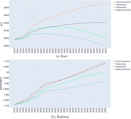
Behavioural, socioeconomic, policy, and technological developments, as well as planned investments, lead to distinct demand developments. This paper estimates the yearly passenger transport demand for the evening peak hours because the demand is the highest during this period. Figure 4(a,b) demonstrate the passenger demand developments until 2050 for the four scenarios.

Figure 4. Passenger demand changes. (a) Road. (b) Railway.

4.1.1. Railway network

Railway investments (in 2025, 2027, 2028, 2029, and 2030) increase the passenger train frequencies of high-frequency trajectories, which induce passenger demand to different extents for each scenario (Figure 4(b)). This explains the irregular demand changes between 2024 and 2031. However, road investment effects on passenger demand are not recognisable in the overall train passenger developments, yet slightly reduce the passenger railway demand due to the extra road capacity and the induced road demand. Figure 5 shows outward passenger demand in 2050 at the network level for the four scenarios.

Figure 5. Railway network passenger demand in 2050 and performance development. (a) Base year demand. (b) Infraconomy demand. (c) Green revolution demand. (d) Missed-boat demand. (e) Safety revolution demand. (f) Railway GJT.

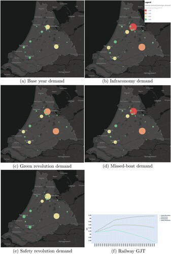
Although socioeconomic, behavioural, and technological determinants develop distinctly for each scenario, the railway passenger demand has an increasing trend in all scenarios. That is mainly explainable by the developments of the generalised journey time (GJT, Figure 5(f)), which has the highest elasticity among all demand determinants. GJT decreases from 2030 for all scenarios except for Missed-boat, which leads to a railway demand increase. The demand increase in the Missed-boat scenario slows down from 2030, which can be attributed to its GJT increase.

After that, train punctuality and population have the most noticeable effects on railway passenger demand. Train punctuality increases for all scenarios except for Infraconomy. However, a high population increase balances the punctuality decrease. The effect of the positively affecting demand determinants is higher than the population decrease effect. The small increase in train ticket prices has a limited impact on the demand trend despite its high demand elasticity value. Notwithstanding the different scenario trends, income and the number of commuting jobs have a comparable absolute but opposite effect on demand. Income increases in all scenarios (Infraconomy the highest), which uplifts the demand.

On the other hand, commuting jobs decrease in all scenarios limiting demand increase. This partly explains the lower demand levels for the Green and Safety Revolution. Representative energy price and vehicle ownership increases have a limited impact on demand. Energy price starts decreasing in 2044 in Green Revolution and, thus, has a more noticeable dampening effect on passenger demand (Figure 4(b)).

4.1.2. Road network

Regarding the effects of planned investments on the road network, Figure 4(a) shows that new roads induce passenger demand more noticeably than road extensions in 2026, 2027, 2028, 2030, and 2036. Planned investments, specifically before 2031, either accelerate the pace of demand increase (Infraconomy and Green Revolution) or change the trend into an increasing demand change (Missed-boat and Safety Revolution). The effect of road extension in 2036 on demand at the presented level of aggregation is limited. Unlike road network investments, railway investments do not show detectable effects on the overall road demand (Figure 4(a)). However, these investments result in railway-induced passenger demand, increasing the train GJT and road demand. This increase is limited because of low GJT road demand elasticity.

Next to the effect of planned investments, scenarios depict different socioeconomic and behavioural developments that lead to an increasing demand trend in Infraconomy and Missed-boat and a decreasing trend in Green and Safety Revolution. These trends can be understood by the extent of changes in demand determinants and the sensitivity of road passenger demand to these changes. Congested travel time has the highest effect on demand. Travel time has a slowing effect on demand increase in Infraconomy and Missed-boat while adding to the demand in Green and Safety Revolution.

Other decisive demand determinants are vehicle ownership and commuting jobs. For Infraconomy and Missed-boat, the high level of vehicle ownership counterbalances the demand decrease due to the (slow) decrease of commuting jobs. On the other hand, a steeper decrease in commuting jobs balances out the moderate and low vehicle ownership increase in the Green and Safety Revolution. GDP and population then have tangible effects on the scenarios' demand.

The moderate GDP change of the Missed-boat and Safety Revolution is noticeable in the different demand levels compared to their counterparts with similar demand trends. The higher GDP development even leads to temporarily higher demand in the Green Revolution than in Missed-boat, despite the higher population increase in the latter scenario. The high population increase in Infraconomy and Missed-boat strengthens the demand increase, while the population drop after 2030 in Green and Safety Revolution decreases passenger demand. The representative energy price increases in all scenarios except for the Green Revolution.

4.2. Freight transport demand

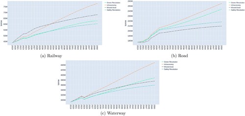
Socioeconomic and technological changes included in the four scenarios, as well as the planned road and waterway investments, shape freight demand. In this paper, the yearly freight transport demand is estimated. Figure 6(a–c) demonstrate the freight demand developments until 2050 for the four scenarios.

Figure 6. Freight demand changes. (a) Railway. (b) Road. (c) Waterway.

4.2.1. Railway network

New road segments attract a share of railway cargo demand in 2024 as road network transport time decreases and makes this network attractive. Although the extra road network capacity reduces railway freight transport, it does not change the increasing demand trends. This is the case for waterway and port investments, which have local effects.

Among all freight demand determinants, the share of service-sector GDP (GS) has the highest impact on demand. It shows the highest increase in Infraconomy and Green Revolution, followed by Safety Revolution and Missed-boat. It partly causes a higher demand in the Missed-boat scenario compared to the other scenarios despite the moderate economic developments (GDP and world trade). It decreases demand for Infraconomy and Green Revolution -with more prosperous national and international economic developments. However, over time, the effects of economic growth become more dominant and lead to more freight demand for Infraconomy and Green Revolution compared to Missed-boat and Safety Revolution.

Representative energy prices positively affect the railway freight demand by shifting demand from road to rail due to road transport's more sensitive and quicker response to price changes. The missed-boat scenario has the highest freight demand since energy prices increase the most. Transport time has a noticeable demand elasticity. Congested travel time on roads and transport time on waterways -a combination of travel time, lock waiting time, and service time of bridges intersecting with waterway segments- have local effects on railway demand. Vehicle load capacity and factors (transport efficiency), demand, and planned investments affect transport time on the road and waterway networks.

4.2.2. Road network

Planned investments in the road network push the road freight demand upwards, with demand jumps in the first ten years (Figure 6(b)) due to extra capacity provision. Like railway freight demand, economic variables (GDP, GS, world trade) explain the demand changes to a large extent. Infraconomy with the highest increase in economic variables balances out the GS increase and generates the highest demand. Green Revolution follows Infraconomy, with similar GS developments and slightly lower economic growth.

Missed-boat and Safety Revolution have similar changes in economic variables but show different demand levels (around 5% difference). This is partly because of the higher energy prices increase in the Missed-boat scenario, which reduces the demand the most among all scenarios. Furthermore, transport time on the road network increases in Missed-boat and Infraconomy (see the last paragraph of Section 4.2.1), which negatively affects road freight demand due to more congested roads. Transport time on waterways also increases, which positively affects road freight demand. In the Green and Safety Revolution, transport time on roads and waterways decreases, reinforcing the demand for these two networks.

4.2.3. Waterway network

Similar to the railway freight demand (Section 4.2.1), new road segments in 2024 attract waterway demand and cause a dip in demand developments due to the provided extra capacity and enhanced transport time. Moreover, waterway and port investments impact waterways freight demand locally. Economic variables mainly shape the demand developments of waterways, similar to the other networks. In the long run, the demand corresponds to the order of the scenarios' GDP and world trade developments.

In the first twenty years, the low GS growth, high energy price, and more congested roads contributed to a higher waterway freight demand for Missed-boat compared to Green Revolution, regardless of the stronger GDP and world trade developments in Green Revolution. Similar reasoning holds for the Missed-boat and Safety Revolution demand difference. Next to economic variables, high energy prices -which affect road transport and deter freight demand- and congested roads contribute to the demand increase and counterbalance a slight waterway transport and GS increase -the two latter variables decrease demand.

4.3. Infrastructure performance

4.3.1. Environmental performance

Figure 7(a–f) demonstrate each transport infrastructure's CO${}_2$ emission and energy consumption. Infraconomy has the worst, and Green Revolution has the best environmental performance. Emission and energy consumption have decreasing trends in all scenarios and all networks. The only exception is the waterway network in Infraconomy.

Figure 7. Environmental performance changes. (a) Railway CO${}_2$ emission. (b) Road CO${}_2$ emission. (c) Waterway CO${}_2$ emission. (d) Railway energy consumption. (e) Road energy consumption. (f) Waterway energy consumption.

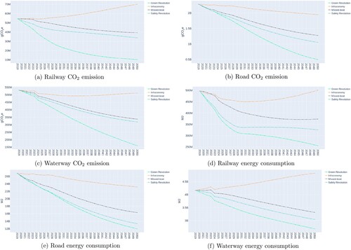
In order to be able to understand the developments, we need to consider fuel mix, transport demand, and emission and energy consumption factors. For all scenarios, shifts occur towards cleaner energy resources, leading to a potential emission and energy consumption decrease. However, transport demand changes affect environmental performance as well. Passenger transport demand increases for Infraconomy and Missed-boat leading to lower environmental performance. This is also the case for railway passenger demand of the Green and Safety Revolution. Since the freight demand increases for all scenarios. Emission and energy consumption are lifted upwards.

Other decisive variables for environmental performance are technological advancements in vehicles, energy production, and distribution. Technological advancements in vehicles reduce tank-to-wheel (TTW) emissions, while efficiency enhancements in energy production reduce the well-to-tank (WTT) emissions. TTW and WTT emissions decrease for all energy resources and scenarios. However, for the Green Revolution scenario, the impact of cleaner energy production and fuel mix change towards cleaner energy sources counterbalances the slight increase in pcu passenger demand till 2031. This leads to a continuous and swift improvement of environmental performance. The drastic shift towards environmentally friendly energy sources decouples pcu-e transport from emission.

In Infraconomy, technological advancements contribute to lower emission and energy consumption, but emission and consumption levels remain high compared to the other scenarios. The transition to cleaner energy resources and vehicles and energy production technology progressions cannot counterbalance the transport demand increase. Energy production in this scenario mainly depends on fossil fuels. Missed-boat and Safety Revolution perform between the other two scenarios. This can be attributed to lower freight and passenger demand levels, on the one hand, and moderate technological advancements and transition to cleaner energy sources, on the other hand,. There is still a noticeable dependency on fossil fuels in these two scenarios. Safety Revolution performs better than Missed-boat due to its faster vehicle and energy production technological advancements and diffusion.

Finally, the effect of planned investments on environmental performance can be seen in the first ten years. These effects are more traceable in Infraconomy and Missed-boat due to their higher demand changes arising from investments. Emission and energy consumption of the railway and road network increase due to higher passenger train frequency and road network capacity. On the other hand, the waterway network shows a drop in emission and energy consumption in 2024, which can be related to the demand shift from this network to the road network in response to newly built road segments.

4.3.2. System performance

Railway GJT (Figure 5(f)) indicates railway service because GJT includes the effect of crowdedness, train frequencies, and capacities on railway passenger demand. In the first ten years, extra capacity through higher railway frequency induces demand, pushing GJT upwards. This push is the highest for Missed-boat with a low train capacity increase and high potential demand. GJT remains almost the same in the Green Revolution scenario after railway investments. In this scenario, the high train capacity increase stabilises the GJT. For all scenarios, train capacity seems to develop sufficiently to the GJT, which remains higher than the base year for Infraconomy and Safety Revolution. However, in Missed-boat, GJT increases after that and reaches a turning point around 2050.

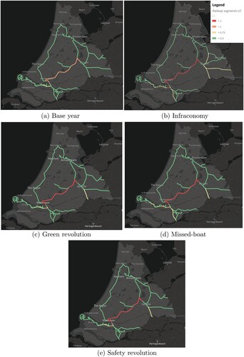
Figure 8 demonstrates the railway freight intensity-capacity ratios at the network level. The increasing trend in railway freight demand is reflected in the railway freight I/C growth in all scenarios compared to the base year. In Infraconomy, the network functions near-capacity since it has the highest freight demand among all scenarios. Green and Safety Revolution are comparable despite their slightly different railway freight demand. Missed-boat is likely to have less available track capacity for freight trains in the Rotterdam province and southern freight corridors compared to Green and Safety Revolution.

Figure 8. Freight I/C of railway segments in 2050. (a) Base year. (b) Infraconomy. (c) Green revolution. (d) Missed-boat. (e) Safety revolution.

Figure 9 presents the road delay factor for the four scenarios in the base year and in 2050. Newly added road segments are circled in Figure 9(c). Road passenger demand and freight passenger car unit equivalent (pcu-e) demand affect road segments' transport time, hence the delay factor. The latter variable depends on road freight demand and transport efficiency -a combination of load capacity and factor change.

Figure 9. Road network delay factor in 2050. (a) Base year. (b) Infraconomy. (c) Green revolution. (d) Missed-boat. (e) Safety revolution.

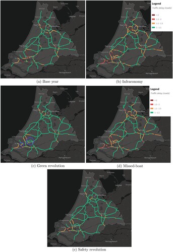
Green Revolution shows enhancements in both national- and regional-level delay due to its long-term passenger demand decrease and transport efficiency increase. Higher transport efficiency balances out freight demand increase. Infraconomy seemingly ends up in a future with a more congested road network.The high transport demand in Infraconomy is the dominant factor causing the highest congested road network among all scenarios. The road network in the Missed-boat scenario demonstrates a similar network-wide delay. However, this scenario has a lower delay for some regions (e.g. around Amsterdam municipality) caused by a lower transport demand. Safety Revolution has the least congested road network -yet close to the Green Revolution- due to its low transport demand.

Figure 10 shows the I/C ratio of the waterway network in the base year and 2050. In all scenarios, the load capacity and factor increase reduce the number of representative vessels, while the rising freight demand counteracts this trend. In the Green Revolution scenario, this leads to lower I/C ratios in 2050 compared to the base year since transport efficiency grows faster than the uplifting effect of freight demand. Infraconomy reaches I/C ratios in 2050, similar to the base year, despite the high freight demand. The higher load capacity and factor seem to balance out the need for more vessels. Missed-boat and Safety Revolution show local I/C ratio differences compared to the base year around the Port of Rotterdam (increase) and Utrecht (decrease), respectively. Table 11 presents four lock complexes in the case study region with the highest I/C ratios. Missed-boat, Infraconomy, and Safety Revolution have comparable intensity-capacity ratios. Despite the different freight demand and transport efficiency (load capacity and factor) developments, this trend can be seen in all scenarios. The transport efficiency enhancement in the Green Revolution leads to the lowest intensity-capacity ratios among all scenarios and counterbalances the freight demand increase -it has the second-highest demand in 2050.

Figure 10. Waterway network intensity-capacity ratio in 2050. (a) Base year. (b) Infraconomy. (c) Green revolution. (d) Missed-boat. (e) Safety revolution.

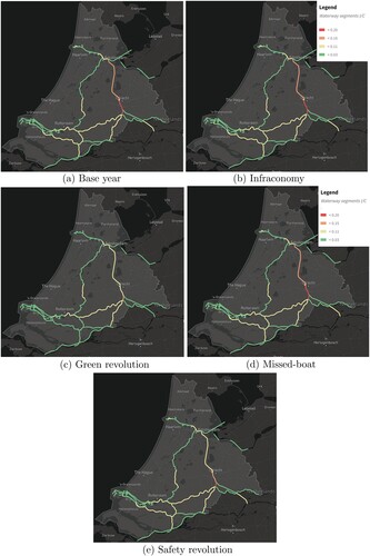
Table 11. Lock I/C ratios in 2050.

Lock name	I/C
	Infraconomy	Green Revolution	Missed-boat	Safety Revolution
Algemene Begraafplaatssluis	0.35	0.24	0.36	0.34
Grote Merwedesluis	0.35	0.24	0.36	0.34
Grote sluis Vianen	0.26	0.18	0.27	0.26
Prinses Beatrixsluizen	0.29	0.20	0.30	0.28

4.4. Result validation

We compared our results with the outcomes of a recent Dutch National long-term transport demand forecast model (LMS) (see Table 12). Infraconomy is the closest scenario to the High WLO scenario of this model, which shows similar socioeconomic developments and also sketches a future with the highest demand increase among the included scenarios. The Dutch infrastructure ministry IenW (2021a, 2021b, 2021c) published a recent set of passenger and freight demand developments based on the LMS, which we use for result comparison. The benchmark results represent passenger and cargo demand for the three Dutch provinces of Noord-, Zuid-Holland, and Utrecht, as well as all freight corridors. Our case study region covers the most populated parts of these provinces. Moreover, the case considers major external national and international freight destinations by including the highest freight volume in the base year OD matrices. Therefore, Infraconomy and the High WLO scenario address similar passenger and freight attraction and generation zones.

Table 12. Results' comparison with national models.

Demand indicator (index)	2030 & 2050		Difference (%)
	Infraconomy	High WLO
Railway Freight	130, 180	135, 176	$-4,+2$
Railway passenger	125, 154	129, 164	$-3,-6$
Road Freight	119, 144	115, 140	$+3,+3$
Road passenger	125, 145	114, 135	$+10,+7$
Waterway Freight	117, 154	121, 143	$-3,+8$

In the case of road transport, LMS calculations include all roads, while the presented case study covers primary and some secondary roads managed by the national road agency. Furthermore, High WLO and Infraconomy scenarios differ in a subset of demand and performance determinants. Despite the overall storyline alignment, the number of commuting jobs, income, vehicle load capacity and factor, and train punctuality have different quantitative developments in both scenarios. Moreover, population developments in Infraconomy (at the municipality level) are not updated based on the recent High WLO projections due to data unavailability.

Another difference between these two scenarios is that the presented model estimates passenger evening peak demand. Finally, the planned investments included are limited to the ones changing the capacity of assets and occur within the boundary of the case study region. These investments affect demand and performance, while planned investments in the benchmark analysis go beyond our investment list. The future infrastructure networks have different structures and states in Infraconomy and High WLO, which lead to different regional and network-level impacts of planned investments on demand developments. These can partly explain the differences in the results Table 12.

Stakeholder engagement facilitates information exchange, knowledge, and expertise in the modelling and validation process (Voinov et al., 2016). For this study, we engaged with a panel of five asset managers from Dutch transport (including port) and energy agencies to define the model design and scope, verify modelling elements (e.g. input data in three scrum sprints), and result presentation and applicability validation. It was concluded that the model can encourage cross-sectoral discussions about demand and performance developments under different plausible scenarios.

Moreover, the effects of planned investments can be traced to interconnected infrastructure networks, which facilitate the identification of possible performance bottlenecks and appropriate responses across sectors. In this way, possible (sometimes identified) different investment possibilities can be examined, and their impacts can be discussed collectively by including the affected infrastructure agencies. A mentioned improvement to the model could be considering a range of vehicle capacity classes affecting network flow and the I/C ratio of segments.

5. Discussion

In the following, we discuss the insights the proposed model generates in terms of the cross-network effects of sector-specific planned investments and sector-specific investments needed under future scenarios. Specifically, we will show that intermodal demand and performance dynamics can be better understood by including various socioeconomic variables reflecting plausible behavioural, policy, and technological developments of specific scenario narratives. We will also discuss how the proposed model enables tracing the interaction among planned investments, demand, and performance developments under various scenarios and across infrastructure networks.

Dynamic interactions arise differently in the scenarios due to changes in the physical systems, local and network-wide capacity provisions, induced demand effects, and policy drivers such as remote working, energy resource taxation, and technological advancements in the energy transition context. Consequently, the model generates more realistic insights into the possible future system-of-systems states and can support the identification of those investments that can enhance infrastructure performance across networks balancing trade-offs between the performance requirements of the individual and the overall network.

5.1. Effects of planned investments across networks

5.1.1. Railway network investments

The effects of railway investments are mainly noticeable in the railway network. Increasing train frequency of high-frequency trajectories induces railway passenger demand (Figure 5(f)). Depending on train capacity in each scenario, such induced demand can increase GJT and affect passenger convenience. In the case of a GJT decrease -due to a sufficient train capacity, increase-planned investments in rail can attract trips from the road network.

On the other hand, where GJT increases in response to the slow development of the passenger train capacity, passenger road demand increases, intensifying the road network congestion in cases where measures to manage the road transport demand are limited. Consequently, a cyclic shift from road to rail and vice versa can be expected when demand management measures and train capacity increase fail to enhance travel time (or GJT). Such shifts -at a certain point in time and with no major intervention- probably do not enhance the overall experienced level of service provided by road and railway networks, as they are likely to function near their capacity.

These higher-order effects of railway investments should be seen together with road network investments. Extra road capacity balances a possible road network congestion increase arising from the mentioned higher-order effects and limits of passenger and freight transport mode change. The extent of this balance depends on the developments of road transport demand, which utilises available capacities. The higher the demand increase rate, the lower the road network capacity to absorb the higher-order demand changes due to planned investment in the railway network. Our results suggest that next to train frequency, a proportionate train capacity development seems to play a significant role in allowing more convenient customer transport, a better railway service, and minimising unintended mode shifts.

5.1.2. Road network investments

Road network capacity investments have a twofold effect. On the one hand, they reduce congestion in the road network by adding capacity. This extra capacity balances out possible congestion increase from the railway passenger mode shift (Section 5.1.1). On the other hand, road investments can lead to more congestion since they attract demand from other modes. Particularly freight demand for rail and waterways (Figure 6(a,c)) shows a dip when major new road connections are open. This leads to fewer freight-carrying trains and vessels -thus, less I/C for the corresponding transport segments. The freight demand shift from the waterway network counterbalances the waterway freight demand increase due to the additional lock capacity provision.

In the long term, road investments have different effects in each scenario (Figure 9). In Infraconomy and Missed-boat, congestion enhances for a few road segments, while the congestion state exacerbates around the major industrial and residential regions. In contrast, the Green and Safety Revolution scenarios have a less congested road network. In all scenarios -despite their relative differences- the road transport delay enhancements are limited for the region around Rotterdam, where the biggest Europe port is situated. That can be explained by the freight demand developments and demand attractions due to the planned investments.

5.1.3. Waterway network investments

The waterway network investments increase the capacity of a port terminal and a lock complex by 30%. The resulting demand increase affects all modalities, with the least impact on the waterway network due to its relatively low I/Cs. Depending on the different scenario development pathways, the increase is absorbed by other modes or adds to the road network congestion. Road investments around the port terminal provide more capacity and buffer for the demand shifts. Road congestion is expected to become more problematic in Infraconomy and Missed-boat due to higher demand, slower load capacity, and factor increase. Green and Safety Revolution are likely to absorb better the road freight demand increase arising from the terminal expansion due to higher transport efficiency and lower freight development.

A 35% increase in lock capacity, part of the southern waterway corridor in the case study region, reduces the lock I/C by 28% for Green Revolution and 25% for the other scenarios. The difference can be explained by the higher transport efficiency in the Green Revolution and higher demand shifts resulting from the lower level of road congestion. The additional lock capacity attracts more freight demand from other networks, especially in the relatively higher road network congestion scenarios. This demand shift occurs within the southern freight corridor where the lock is located but remains limited as the lock I/C is already low before the extension investment.

5.2. Sector-specific investments under different scenarios

5.2.1. Green revolution

Railway GJT decreases while passenger demand grows in the long run, which provides the opportunity for encouraging more passenger mode shifts. Such a shift can further enhance road network performance. Railway investments should enable larger trains and make railway infrastructure suitable for such trains based on increased passenger train capacity. For instance, railway track width might be needed to increase, or a higher load-bearing capacity of track foundation. The railway freight I/C suggests possible investments to provide extra capacity for tracks connecting the regions of Rotterdam and Utrecht.

Because of the continuous freight demand growth, part of the railway tracks in the Rotterdam region intersecting with south-north and east-west corridors can become capacity bottlenecks. Utilising longer freight trains, increasing the allowable maximum train speed, and providing more railway infrastructure to create extra capacity can be examples of investments that can resolve capacity bottlenecks. Due to environmentally driven priorities and relatively high economic growth, such investments will likely be considered and realised in the Green Revolution. The stabilising railway freight demand growth, resulting from a further economic shift towards knowledge and service economy and local production, can keep the I/C ratio constant and, thus, limit the required capacity extension in the long run.

Road network performance will enhance until 2050 (Figure 9(c)) due to the combined effect of passenger transport demand decrease, transport efficiency enhancements, and extra capacities provided by planned investments. Hence, required road infrastructure expansions can be limited to a few connections around some major industrial and urban municipalities -especially Rotterdam. Alternatively, the projected performance development could be tolerated as the decreasing trend of transport demand further reduces congestion.

In this scenario, cleaner vehicles and their supporting infrastructure become available and affordable, which allows for longer-range travel. This can lead to a rebound effect. Road transport can be associated as a clean mode of transport and lead to more trips and might create congestion (Seebauer, 2018, Font Vivanco et al., 2014). The possible high level of (semi)autonomous vehicles has a twofold effect. This can increase congestion in urban areas while decreasing congestion on highways (Snelder et al., 2019, Pernestål and Kristoffersson, 2019). The former effect can be explained due to the possible mode shifts and enhanced accessibility, while the latter can be attributed to greater transport efficiency and improved driving behaviour. Overall, investments should be geared towards the control of possible demand rebound effects.

The I/C ratio of waterways decreases in this scenario despite the freight demand increase. That can be explained by the load capacity and factor increase and freight transport shift in response to planned investments in road infrastructure. The available capacities allow for a mode shift from roads to waterways, enhancing the road network performance. Such possible performance enhancement can be of added value to the port authorities in Rotterdam and Amsterdam, leading to better freight distribution. Similarly, the I/C ratio of locks remains far below the critical level of 0.6, at which investments are required to increase locks capacity (Koedijk, 2020). The estimated waterway performance is based on representative vessels and their transport efficiency developments. Waterways and terminals might need investments to allow these vessels safe and reliable passage and service. This might include minimum available passage depth and headway.

In the Green Revolution scenario, investments accommodate the need for renewable energy generation and charging infrastructure, e.g. fast-charging stations (CAT, Climate Action Tracker, 2021a). Due to the decrease in long-term infrastructure utilisation, maintenance investments are expected to decline. Replacement investments can be coupled with functional improvements, such as enabling charging while driving. Transport emissions decreased drastically, aligned with the Green Revolution's main driver. This scenario successfully reduces emissions and energy consumption due to its fast and extensive transition towards cleaner energy resources.

5.2.2. Infraconomy

Railway GJT (Figure 5(f)) in 2050 is higher than in the base year but seems to decrease in the long run. This suggests that passenger convenience worsens, which can be approached by a combination of service improvements or tolerating it until the decreasing trend of GJT comes into effect. Service improvements can include a faster transition to higher capacity trains and higher train frequencies between nodes with high passenger railway demand (Figure 5(b)). It is important to combine the mentioned measures because train frequency increase with insufficient train capacity provision may not respond properly to the induced demand. Investments should be made to provide larger trains and to adapt the railway network for the safe and reliable flow of these trains.

Railway freight I/C developments require intervention similar to the Green Revolution. Important differences are the higher train intensities and the extent of railway tracks functioning beyond available capacities. More capacity provision interventions are probably required in the Rotterdam region, where important freight corridors intersect. Because of the high railway freight demand, combining interventions (as mentioned in the Green Revolution paragraph, Section 5.2) seems more effective. Available waterway capacity can release the pressure from the railway network and give more room and time for capacity enhancements.

Further decrease in GJT can cause a mode shift from road passenger demand, where a high level of congestion is expected (both in the order of magnitude and spatial extent, Figure 9(b)). Hence, capacity extensions seem to be necessary. This is in line with the dominant economy-driven mindset of Infraconomy, which prefers infrastructure expansions above other measures, such as efficiency enhancements. Investments can take place around the main four urban and industrial areas and the south-north and east-west cargo trajectories. Because of higher capacity utilisation, a faster and more severe condition decline is probable for the road network. Thus, more frequent maintenance investments become likely.

However, a continuous increase in transport demand, combined with the mentioned investment strategy, impedes compliance with the required safety and noise levels. By modifying the infrastructure layout or implementing intelligent ICT solutions for both vehicles and infrastructure, the road network can become safer (Palkovics and Fries, 2001, Rahman et al., 2019). A sharp increase in noise and pollution can limit infrastructure expansion investments and prevent resolving capacity bottlenecks.

The I/C ratio of waterways stays at similar levels as in the base year despite a high freight demand increase. It is worth mentioning that the transport efficiency increases caused such an I/C ratio trend. Smaller or less efficient transport can increase the lock and waterway I/C. Similar to Green Revolution, the available capacities allow for a mode shift from congested roads to waterways. Such a shift can reduce emissions and energy demand, as road transport remains highly polluting due to the slow transition towards cleaner energy resources.

Technological advancement and transition to cleaner energy resources in the Infraconomy scenario modestly affect the emission and energy consumption. Environmental performance can worsen long-term without any measure to control and shift transport demand. Consequently, reaching climate goals set by the European Union to keep the temperature increase of ${1.5}^{\circ }$ Celsius remains extremely challenging (CAT, Climate Action Tracker, 2021b). Thus, this scenario is expected to be confronted with the most adverse impacts of climate change on infrastructure in the long term. Such hindrances probably disrupt transport, energy provision, distribution, and storage, which can have substantial economic implications. Thus, the high economic growth visioned in Infraconomy can face challenges and seem not to be sustained in the long run; hence, Infraconomy can be transformed into a scenario with lower economic growth (similar to Missed-boat). Thus for more long-term analysis (e.g. until 2100), economic development assumptions should be corrected to consider such possible trend changes.

5.2.3. Missed-boat

Railway GJT (Figure 5(f)) is the highest among all scenarios in 2050 and probably remains high in the long run. Hence, service improvements seem necessary to deal with the growing passenger demand and slow train capacity increase. This may include combined measures of a faster transition to higher capacity trains and train frequencies. Like in Infraconomy, considering combined measures is necessary to cope with the demand increase. However, scarce financial resources can impede timely and effective measures to enhance passenger railway service. Railway freight I/C develops similarly to the Green Revolution. Hence, similar interventions are likely to be needed.

The capacity utilisation in the Rotterdam region and part of the southern corridor can become more critical from the capacity perspective. Capacity utilisation is higher in this scenario, caused by higher freight demand. Capacity investments might face hurdles because of slow economic growth and a segmented political atmosphere; thus, railway freight flows can be disrupted where capacity investments are limited and hold back (slow) economic growth. Like in Infraconomy, mode changes to waterways can reduce train intensity and enhance the railway network capacity utilisation.

The road network performs slightly better (with some exceptions around the Rotterdam municipality) compared to the base year. As Figure 9(d) shows, road congestion only occurs in the four major industrial and urban regions in 2050. However, the performance is expected to worsen due to increased transport demand. Consequently, road network capacity extensions will probably become necessary. Moreover, relatively high levels of road usage require maintenance investments, including functional performance improvements accommodating the increasing demand, minimising noise, and enhancing safety.

The I/C ratio of waterways slightly increases in this scenario (e.g. in the Rotterdam region) due to slow transport efficiency improvements. The waterway capacity availability allows for the mode shift from the congested road network. Like Infraconomy, this shift is not preferable in Missed-boat from the perspective of environmental performance indicators. Financial resources are limited in the Missed-boat scenario, which makes investments less likely. This can lead to less efficient transport and smaller vessel utilisation, which increases the waterway, locks I/C and limits possible mode shifts to the waterway network.

In the long run, high emission levels can worsen the occurrence and intensity of extreme weather events arising from climate change. This will require measures to guarantee continuous and desired infrastructure functionalities. However, implementing the required countermeasures might be challenging because of this scenario's unstable and fragmented policy sphere and weak economic growth. This can create a lock-in situation and reinforce infrastructure functionality disruptions and bottlenecks.

5.2.4. Safety revolution

Railway GJT is similar to the Infraconomy scenario's GJT, although both scenarios follow different behavioural, socioeconomic, and technological developments. In this scenario, railway passenger demand develops more slowly, and financial capacity is limited due to moderate economic growth. Hence, tolerating the increased GJT -until the decline sets in and service improvements occur- becomes a more feasible strategy than a proactive strategy to enhance passenger railway service. Transport demand decrease in the long term reduces the likelihood of capacity expansion needs. Consequently, the adverse effects of accidents, noise, and pollution are smaller, and tackling them becomes less critical and challenging compared to Infraconomy and Missed-boat. Safety Revolution has a relatively swift energy transition. Rebound effects of emergent vehicle types are expected to increase transport demand to a lower extent than the Green Revolution. Railway freight I/C develops similarly to the Green Revolution, requiring similar capacity increases. In contrast, the planning and realisation of such investments can be slowed down because of slow economic growth.

The population shrinks from 2050 in this scenario and decreases the necessity of infrastructure expansion. This allows infrastructure developments (locally, e.g. around the Rotterdam region) and ensures the desired liveability standards. The decrease of the waterway I/C is similar to the Green Revolution (e.g. around Utrecht municipality), which can be explained by the transport efficiency improvements and cargo transport shift because of the road network planned investments. Such low levels of waterway I/C ratio provide opportunities for the mode shift from the road to reduce congestion in critical regions (e.g. around the port of Rotterdam) and further reduce emission and energy demand. Like Missed-boat, investments may not occur sufficiently due to limited financial capacity.

Safety Revolution will likely have fewer emissions and energy consumption than Missed-boat and Infraconomy. However, it remains to perform in the neighbourhood of the former scenario despite a faster transition towards cleaner energy resources. Thus similar to Missed-Boat, it is likely that Safety Revolution faces climate-related impacts in the long run. However, the well-being-oriented mindset of Safety Revolution, more available space, and lower population can better facilitate the design and implementation of required mitigation and control measures. Financial resources for realising required investments can face limitations due to moderate economic growth. For instance, maintaining and expanding infrastructure to accommodate energy transition or climate change-related mitigation and adaptation investments can be impeded. However, decreased maintenance investments -because of less utilised infrastructure- can provide infrastructure agencies with extra capital and resources.

6. Policy implications

In addition to investment-related decisions, the developed model can assist in defining policies that give shape to certain futures. Policies directed at managing transport demand, enhancing efficiency, and encouraging behavioural and technological transition towards cleaner energy sources are covered in this research. Such policies affect demand and infrastructure performance and can have different implications on the effectiveness of investments.

For instance, the considered measures increasing the vehicles' capacity and efficiency, demand management, and pricing leverage affect the degree of remote working, transport fuel mix transitions, and emission and energy usage efficiency enhancements -due to technological developments and dispersion in energy and transport industries. This, in turn, affects environmental performance by reducing emission and energy consumption and transport performance by enabling reliable and safe passenger and cargo transport. Furthermore, planned investments' effectiveness can be better ensured, possible expansion and maintenance investments can be limited, and more room for investment shifts to accommodate emerging socioeconomic trends and technologies can be created.

Another high-level policy factor is the economic structure change towards the service- and knowledge-based economy, potentially decreasing freight demand. World trade is more prevalent for international freight demand than national freight demand. The impact of economic structure change depends on global-scale developments. We partly included the effect of the shift in the economic structure; however, a more thorough investigation is required to gain better insights into the possible influences.

It is important to stress that depending on the dominant policies and infrastructure performance states, transport mode shift possibilities enable resolving performance bottlenecks. In all scenarios, waterways provide available capacity for mode change. However, lock capacities become critical sooner than waterways, and locks can create capacity bottlenecks. Furthermore, a combination of vessel capacity and transport efficiency increase can effectively resolve possible capacity bottlenecks in the waterway network. In addition to that, in scenarios with more environmentally performing road networks -in the case of available capacity-mode shifts can be encouraged to resolve capacity impediments in the other networks.

7. Conclusions

This research proposes a scenario-based system-of-systems model to advance existing modelling approaches for infrastructure investment planning and appraisal. The proposed model improves investment decision-making by focusing on infrastructure performance outcomes of sector-specific decision-making and planning. It enables tracing and evaluating the effects of planned investments and distinct behavioural, socioeconomic, policy, and technological developments on the demand and performance of functionally and spatially interconnected infrastructure. These effects can be assessed both locally (to the affected assets) and globally (the whole case study region), as well as for the short-term (a few years after the investment actualisation) and the long-term. Here, plausible scenarios address future uncertainties.

The model also enables the enhancement of infrastructure performance across networks rather than only paying attention to the stand-alone benefits of sector-specific investments. It provides insights into potential investment needs (e.g. maintenance, capacity expansion) or shifts in investment priorities based on infrastructure demand and performance under different futures. In the light of available funding, such a better understanding of expected infrastructure performance and investment needs can increase the accountability and transparency of infrastructure investment planning (Grant et al., 2013).

The proposed elasticity-based sub-models are suitable for long-term demand and performance estimations. They are an appropriate compromise between the projection of reasonable future developments -as validated in Section 4.4- and low model run times and reduced data collection costs. They include the main demand determinants but are flexible in modifying input parameters, variables, and future states in the physical infrastructure (Jonsson et al., 2011, de Dios Ortúzar and Willumsen, 2011).

The current modelling approach is suitable for small changes in demand determinants between each simulation time step (i.e. in the order of 10%). Since the modelling approach assumes demand determinants to be independent, the future scenarios incorporate a bundle of variables that vary in line with the scenario drivers. Hence, the interaction among demand determinants is considered with the generation and adaptation of each scenario. In future work, regression-based approaches could be used to enhance forecasting precision. However, these approaches require more complex data collection and calibration processes compared to the proposed approach.

In addition to investment-related decisions, the proposed model can support defining and evaluating policies that shape certain futures. Policy examples are demand management and the instruments that encourage a transition to cleaner energy sources and technologies. Policies -specifically those targeting energy transition- require continuous and coordinated responses and actions to guarantee their effectiveness. However, influential policies go beyond the ones considered in the presented model. Carbon and road pricing are important examples of such policy responses, facilitating a faster energy transition. The proposed model can still be used to indirectly reflect on the effects of some of the mentioned measures by including carbon pricing in the fuel price or adjusting vehicle ownership.

Moreover, future works can extend the model to investigate the effects of other mobility behavioural changes, such as the increase in online shopping or mobility as a service. Such effects (e.g. on emission and energy demand) depend on technology advancements and diffusion (determining emission and energy factor and mix). This, in turn, depends on the availability of resources and the political and institutional efforts (nationally and internationally) for timely responses. Then, broader mobility behavioural changes can affect infrastructure demand and performance.

Introduced demand determinants are a source of uncertainties, which can be addressed by assuming variability of dominant factors in line with the qualitative narrative of scenarios. Additionally, all scenarios share the same demand elasticity values, while they remain constant throughout the simulation. In reality, under certain situations, some of the variables' demand elasticity can change (e.g. energy prices). Extracting such elasticity values can be challenging because of the data, model scarcity, and associated uncertainties, as they mainly reflect future choices.

The model can further be extended to give more insights into the effect of uncertainties on demand determinant variables. This can be done by performing sensitivity analyses on variables representing certain technological and policy developments (e.g. vehicle capacity advancements or energy and emission factor changes). This means that decision-makers can better understand the importance of such variables on infrastructure demand and performance.

Next to included performance indicators, broader functional performance indicators such as structural performance and noise emission can give a broader understanding of demand developments and possible performance bottlenecks. Moreover, possible investments can be identified for specific assets, regions, or a certain point in time. It is also important to better understand feedback loops between the out-rolling of emerging passenger and freight vehicle technologies and transport demand.

Future research could investigate the possible behavioural and technological developments responding to policy measures, which pave the path for a more dynamic analysis of long-term infrastructure demand and performance. Lastly, the anticipatory power of the presented model can be extended by including scenarios with fluctuating or trend changes in demand determinants (e.g. economic development). In this way, depicted futures can include pathways that reflect possible disrupting interventions, policies, or events.

Acknowledgments

The authors would like to thank the experts of the infrastructure agencies involved in the knowledge and network organisation Next Generation Infrastructure (NGInfra) for their contributions to the research. The authors would also like to show their gratitude to Harmen Zandman, Arjan Olsthoorn, and Maarten de Jonge from ProRail for facilitating access to data and valuable knowledge exchange.

Disclosure statement

The authors report there are no competing interests to declare.

Data availability statement

Derived data supporting the findings of this study are available from the corresponding author on request.

Additional information

Funding

This work was supported by the Nederlandse Organisatie voor Wetenschappelijk Onderzoek (Dutch Research Council (NWO)) and Next Generation Infrastructures (NGInfra) under Grant 439.16.803.

References

- Ambrosini Christian, Jesus Gonzalez-Feliu, and Florence Toilier. 2013. “A Design Methodology for Scenario-Analysis in Urban Freight Modelling.” European Transport/Trasporti Europei 54 (7): 1–21. 〈halshs-00843286〉.
- Amin Massoud. 2015. “System-of-Systems Approach.” In Intelligent Monitoring, Control, and Security of Critical Infrastructure Systems, 317–354. Springer.
- Annema Jan Anne, Carl Koopmans, and Bert Van Wee. 2007. “Evaluating Transport Infrastructure Investments: The Dutch Experience with a Standardized Approach.” Transport Reviews 27 (2): 125–150. doi:10.1080/01441640600843237.
- Asgarpour S., A. Hartmann, K. Gkiotsalitis, and R. Neef. 2023. “Scenario-Based Strategic Modeling of Road Transport Demand and Performance.” Transportation Research Record. https://doi.org/10.1177/03611981221143377.
- Atilhan Selma, Sunhwa Park, Mahmoud M. El-Halwagi, Mert Atilhan, Margaux Moore, and Rasmus B. Nielsen. 2021. “Green Hydrogen As An Alternative Fuel for the Shipping Industry.” Current Opinion in Chemical Engineering 31: Article ID 100668. doi:10.1016/j.coche.2020.100668.
- Bellsolà Olba X., Winnie Daamen, Tiedo Vellinga, and Serge P. Hoogendoorn. 2015. “Estimating Port Network Traffic Capacity.” Zeszyty Naukowe Akademii Morskiej w Szczecinie 42 (114).
- Bellsolà Olba Xavier, Winnie Daamen, Tiedo Vellinga, and Serge P. Hoogendoorn. 2019. “A Method to Estimate the Capacity of An Intersection of Waterways in Ports.” Transportmetrica A: Transport Science 15 (2): 1848–1866. doi:10.1080/23249935.2019.1652866.
- BIVAS. 2018. “Snelheidsbepaling -- BIVAS.” https://bivas.chartasoftware.com/Home/BIVASApplicatie/Documentatie/Snelheidsbepaling.
- Blainey Simon P., and John M. Preston. 2019. “Predict or Prophesy? Issues and Trade-Offs in Modelling Long-Term Transport Infrastructure Demand and Capacity.” Transport Policy 74: 165–173. doi:10.1016/j.tranpol.2018.12.001.
- Bliemer Michiel C. J., Mark P. H. Raadsen, Luuk J. N. Brederode, Michael G. H. Bell, Luc J. J. Wismans, and Mike J. Smith. 2017. “Genetics of Traffic Assignment Models for Strategic Transport Planning.” Transport Reviews 37 (1): 56–78. doi:10.1080/01441647.2016.1207211.
- Bückmann Ewout, Dries Goffin, Jorrit Harmsen, Tom Scheltjens, and Tessa Sendar. 2009. “Capaciteitsanalyse binnenvaart Scheldegebied.”.
- Burgschweiger Sandra, Axel Wolfermann, and Gernot Liedtke. 2019. “A Macroscopic Freight Transport Demand Model to Analyze Effects of Transport Planning in Germany.” In Proceedings of the 3rd Interdisciplinary Conference on production. Logistics and Traffic ICPLT, Darmstadt, Germany, 25–26.
- Camargo Pedro, Jan Zill, and Andrew O'Brien. 2018. “AequilibraE.” http://www.aequilibrae.com/python/latest/index.html.
- CAT, Climate Action Tracker. 2021a. “Policies & Actions-Transport.” https://climateactiontracker.org/countries/eu/policies-action/.
- CAT, Climate Action Tracker. 2021b. “Targets.” https://climateactiontracker.org/countries/eu/targets/.
- CBS. 2013. “Brandstofverbruik en CO2-uitstoot van personenauto's, 2011*.”.
- CE Delft. 2015. “STREAM personenvervoer 2014.”.
- CE Delft. 2020. “STREAM Freight transport 2020.”.
- Chamberlin Graeme. 2010. “Methods Explained: Temporal Disaggregation.” Economic & Labour Market Review 4 (11): 106–121. doi:10.1057/elmr.2010.157.
- Dahl Alexander, Annette Kindl, and Christoph Walther. 2016. “Methodology Manual for the Federal Transport Infrastructure Plan 2030.”.
- de Bok Michiel, Gerard De Jong, Jaap Baak, Eveline Helder, Cindy Puttemans, Kurt Verlinden, Dana Borremans, et al. 2015. “A Population Simulator and Disaggregate Transport Demand Models for Flanders.” Transportation Research Procedia 8: 168–180. doi:10.1016/j.trpro.2015.06.052.
- de Dios Ortúzar Juan, and Luis G. Willumsen. 2011. Modelling Transport. London: John Wiley & Sons.
- De Jong Gerard, Arnaud Burgess, L. A. Tavasszy, Robbert Versteegh, Michiel de Bok, and Nora Schmorak. 2011. “Distribution and Modal Split Models for Freight Transport in The Netherlands.” In Proceedings of the 2011 European Transport Conference, Association for European Transport. On the Generalized Cost-Demand Elasticity of Intermodal Container Transport.
- de Jong Gerard C., and Odette van de Riet. 2008. “The Driving Factors of Passenger Transport.” European Journal of Transport and Infrastructure Research 8 (3): 227–250. https://doi.org/10.18757/ejtir.2008.8.3.3348.
- Ehrenberger Simone, Stefan Seum, Thomas Pregger, Sonja Simon, Gunnar Knitschky, and Ulrike Kugler. 2021. “Land Transport Development in Three Integrated Scenarios for Germany–Technology Options, Energy Demand and Emissions.” Transportation Research Part D: Transport and Environment 90: Article ID 102669. doi:10.1016/j.trd.2020.102669.
- Font Vivanco David, Jaume Freire-González, René Kemp, and Ester van der Voet. 2014. “The Remarkable Environmental Rebound Effect of Electric Cars: A Microeconomic Approach.” Environmental Science & Technology 48 (20): 12063–12072. doi:10.1021/es5038063.
- Geilenkirchen G. P., K. T. Geurs, H. P. van Essen, A. Schroten, and B. Boon. 2010. “Effecten van prijsbeleid in verkeer en vervoer. Kennisoverzicht.”.
- Geilenkirchen Gerben, Harm ten Broeke, and Anco Hoen. 2016. “Verkeer en vervoer in de Nationale Energieverkenning 2015.” PBL-Planbureau voor de Leefomgeving, Den Haag.
- Grant Michael, Janet D'Ignazio, Alexander Bond, and Alanna McKeeman. 2013. “Performance-Based Planning and Programming Guidebook.”.
- Groen Tsjitske, Jaco van Meijeren, IenW, and DVS. 2010. “Vlootontwikkeling binnenvaart.”.
- Groot Wim, and Henk van Mourik. 2012. “Over Brandstofprijzen En Automobiliteit.” Tijdschrift Vervoerswetenschap 48 (3)): 68–83.
- Henning Arne, Martin Plohr, Doruk Özdemir, Michael Hepting, Hermann Keimel, S. Sanok, and Robert Sausen, et al. 2016. “The DLR Transport and the Environment Project-Building Competency for a Sustainable Mobility Future.”.
- Hilbers H., J. van Meerkerk, D. Snellen, R. Euwals, T. Hendrich, K. van Ruijven, and P. Verstraten. 2020. “ONTWIKKELING MOBILITEIT.”.
- Huizinga Free, and Bert Smid. 2005. “Four Futures of the Netherlands; Production, Labour and Sectoral Structure in Four Scenarios Until 2040.”.
- Hymel Kent M., Kenneth A. Small, and Kurt Van Dender. 2010. “Induced Demand and Rebound Effects in Road Transport.” Transportation Research Part B: Methodological 44 (10): 1220–1241. doi:10.1016/j.trb.2010.02.007.
- IenW. 2020. “Programma Hoogfrequent Spoorvervoer.”.
- IenW. 2021a. “Integrale Mobiliteitsanalyse 2021, Goederenvervoer Integraal.”.
- IenW. 2021b. “Integrale Mobiliteitsanalyse 2021, Hoofdrapport.”.
- IenW. 2021c. “Integrale Mobiliteitsanalyse 2021, Ontwikkeling mobiliteit.”.
- IenW, BZK, and EZK. 2020. “MIRT Overzicht 2021.”.
- Ives Christopher D., Cathy Oke, Ailish Hehir, Ascelin Gordon, Yan Wang, and Sarah A. Bekessy. 2017. “Capturing Residents' Values for Urban Green Space: Mapping, Analysis and Guidance for Practice.” Landscape and Urban Planning 161: 32–43. doi:10.1016/j.landurbplan.2016.12.010.
- Jonsson Daniel, Svante Berglund, Peter Almström, and Staffan Algers. 2011. “The Usefulness of Transport Models in Swedish Planning Practice.” Transport Reviews 31 (2): 251–265. doi:10.1080/01441647.2010.537100.
- KiM. 2017. “Mobiliteitsbeeld 2017.”.
- KiM. 2019. “Mobiliteitsbeeld 2019.”.
- Klein John, and Gerben Geilenkirchen. 2018. “Methods for Calculating the Emissions of Transport in the Netherlands.” Task Force on Transportation of the Dutch Pollutant Release and Transfer Register.
- Knoope Marlinde, and Jan Francke. 2020. “Verklaring Van De Ontwikkelingen in Het Goederenvervoer in Nederland.” Tijdschrift Vervoerswetenschap 56 (2): 1–26.
- Koedijk Otto Christiaan. 2020. “Richtlijnen Vaarwegen 2020.” ISBN 978-90-9033423-3 Rijkswaterstaat Water, Verkeer en Leefomgeving (WVL) Afdeling BNSV.
- Krause Jette, Christian Thiel, Dimitrios Tsokolis, Zissis Samaras, Christian Rota, Andy Ward, Peter Prenninger, et al. 2020. “EU Road Vehicle Energy Consumption and CO2 Emissions by 2050–Expert-based Scenarios.” Energy Policy 138: Article ID 111224. doi:10.1016/j.enpol.2019.111224.
- Kugler Ulrike, Jens Brokate, Christoph Schimeczek, and Stephan Schmid. 2017. “Powertrain Scenarios for Cars in European Markets to the Year 2040.” In TAE Conference Proceedings-11th International Colloquium Fuels.
- Kuiper E., and N. E. Ligterink. 2013. “Voertuigcategorieën en gewichten van voertuigcombinaties op de Nederlandse snelweg op basis van assen-combinaties en as-lasten.”.
- Kupfer Franziska, Hilde Meersman, Evy Onghena, and Eddy Van de Voorde. 2017. “The Underlying Drivers and Future Development of Air Cargo.” Journal of Air Transport Management 61: 6–14. doi:10.1016/j.jairtraman.2016.07.002.
- Litman Todd. 2019. Understanding Transport Demands and Elasticities.” Victoria Transport Policy Institute.
- Lovrić Milan, Simon Blainey, and John Preston. 2017. “A Conceptual Design for a National Transport Model with Cross-sectoral Interdependencies.” Transportation Research Procedia 27: 720–727. doi:10.1016/j.trpro.2017.12.150.
- Maerivoet Sven, and Bart De Moor. 2005. “Transportation Planning and Traffic Flow Models.” arXiv preprint physics/0507127.
- Maier Holger R., Joseph H. A. Guillaume, Hedwig van Delden, Graeme A. Riddell, Marjolijn Haasnoot, and Jan H. Kwakkel. 2016. “An Uncertain Future, Deep Uncertainty, Scenarios, Robustness and Adaptation: How Do they Fit Together?.” Environmental Modelling & Software 81: 154–164. doi:10.1016/j.envsoft.2016.03.014.
- Manders Antonius Jacobus Gerardus, and Clemens Joannes Maria Kool. 2015. “Toekomstverkenning welvaart en leefomgeving Nederland in 2030 en 2050: twee referentiescenario's.”.
- Matthias Volker, Johannes Bieser, Tudor Mocanu, Thomas Pregger, Markus Quante, Martin O. P. Ramacher, Stefan Seum, and Christian Winkler. 2020. “Modelling Road Transport Emissions in Germany–Current Day Situation and Scenarios for 2040.” Transportation Research Part D: Transport and Environment 87: Article ID 102536. doi:10.1016/j.trd.2020.102536.
- Melian Veronica, and Adrian Zebib. 2020. “How Covid-19 Contributes to a Long-Term Boost in Remote Working.” https://www2.deloitte.com/ch/en/pages/human-capital/articles/how-covid-19-contributes-to-a-long-term-boost-in-remote-working.html.
- Mitradjieva Maria, and Per Olov Lindberg. 2013. “The Stiff is Moving – conjugate Direction Frank-Wolfe Methods with Applications to Traffic Assignment.” Transportation Science 47 (2): 280–293. doi:10.1287/trsc.1120.0409.
- Mtoi Enock T., and Ren Moses. 2014. “Calibration and Evaluation of Link Congestion Functions: Applying Intrinsic Sensitivity of Link Speed As a Practical Consideration to Heterogeneous Facility Types Within Urban Network.” Journal of Transportation Technologies 4 (2): 141–149. https://doi.org/10.4236/jtts.2014.42014.
- MuConsult. 2015. “Literatuurstudie tijd- en conveniencegevoeligheden openbaar vervoer.”.
- NDW. 2020. “Nationaal Dataportaal Wegverkeer.” https://www.ndw.nu/.
- Neef Robin, Stefan Verweij, Tim Busscher, and Jos Arts. 2020. “A Common Ground? Constructing and Exploring Scenarios for Infrastructure Network-of-Networks.” Futures 124. https://doi.org/10.1016/j.futures.2020.102649.
- Nijland Hans, Gerben Geilenkirchen, and Hans Hilbers. 2019. “Achtergrondrapport bij effectschattingen mobiliteits-maatregelen klimaatakkoord.”.
- NS. 2022. “Treinen van NS.” https://www.ns.nl/over-ns/treinen-van-ns.
- Palkovics László, and Ansgar Fries. 2001. “Intelligent Electronic Systems in Commercial Vehicles for Enhanced Traffic Safety.” Vehicle System Dynamics 35 (4–5): 227–289. doi:10.1076/vesd.35.4.227.2044.
- PBL, CBS, TNO, and RIVM. 2017. “Klimaat-en Energieverkenning 2017.”.
- PBL, CBS, TNO, and RIVM. 2020. “Klimaat-en Energieverkenning 2020.”.
- PDOK. 2020. “PDOK.” https://www.pdok.nl/.
- Pernestål Anna, and Ida Kristoffersson. 2019. “Effects of Driverless Vehicles: Comparing Simulations to Get a Broader Picture.” European Journal of Transport and Infrastructure Research 1 (19): 1–23. E-ISSN 1567-7141.
- Port of Rotterdam. 2021. “Bouwers gekozen voor aanleg kades Amaliahaven.” https://www.portofrotterdam.com/nl/nieuws-en-persberichten/bouwers-gekozen-voor-aanleg-kades-amaliahaven.
- ProRail. 2021a. “Achtergrond rapport Spoor en BTM.”.
- ProRail. 2021b. “Integrale Mobiliteitsanalyse 2021 Deelrapportage Spoor en BTMIntegrale Mobiliteitsanalyse 2021 Deelrapportage Spoor en BTM.”.
- Rahman Md Hasibur, Mohamed Abdel-Aty, Jaeyoung Lee, and Md Sharikur Rahman. 2019. “Enhancing Traffic Safety at School Zones by Operation and Engineering Countermeasures: A Microscopic Simulation Approach.” Simulation Modelling Practice and Theory 94: 334–348. doi:10.1016/j.simpat.2019.04.001.
- Rijksoverheid. 2020. “Open data van de Overheid.” https://data.overheid.nl/.
- Santén Vendela. 2017. “Towards More Efficient Logistics: Increasing Load Factor in a Shipper's Road Transport.” The International Journal of Logistics Management 28 (2)): 228–250. ISSN 0957-4093.
- Seebauer Sebastian. 2018. “The Psychology of Rebound Effects: Explaining Energy Efficiency Rebound Behaviours with Electric Vehicles and Building Insulation in Austria.” Energy Research & Social Science46: 311–320. doi:10.1016/j.erss.2018.08.006.
- Seum Stefan, Simone Ehrenberger, and Thomas Pregger. 2020. “Extended Emission Factors for Future Automotive Propulsion in Germany Considering Fleet Composition, New Technologies and Emissions From Energy Supplies.” Atmospheric Environment 233: Article ID 117568. doi:10.1016/j.atmosenv.2020.117568.
- Snelder Maaike, Isabel Wilmink, Jeroen van der Gun, Hendrik Jan Bergveld, Parvin Hoseini, and Bart van Arem. 2019. “Mobility Impacts of Automated Driving and Shared Mobility.” European Journal of Transport and Infrastructure Research 19 (4): 291–309. https://doi.org/10.18757/ejtir.2019.19.4.4282.
- TRANSTOOL. 2017. “TRANSTOOL 3-Final publishable summary.”.
- TRANSTOOLS. 2014. “TRANSTOOLS3 -- About.” http://www.transportmodel.eu/about.html.
- U.K. Department for Transport. 2019. “TAG UNIT M4 Forecasting and Uncertainty.”.
- U.K. Department for Transport. 2022. “TAG unit A1-1 cost-benefit analysis.”.
- van Dender Kurt, and Martin Clever. 2013. “Recent Trends in Car Usage in Advanced Economies: Slower Growth Ahead?; Summary and Conclusions.” In International transport Forum, International Transport Forum Discussion Paper.
- van de Riet Odette, Gerard de Jong, and Warren Walker. 2004. “Drivers of Freight Transport Demand Worldwide.” In European Transport Conference,.
- van der Loop Han. 2018. “Effecten van Het Nieuwe Werken op mobiliteit en congestie 2000–2016.”.
- van der Loop H., P. Bakker, F. Savelberg, M. Kouwenhoven, and E. Helder. 2018. “Verklaring van de ontwikkeling van het ov-gebruik in Nederland over 2005-2016.”.
- van der Loop Han, Peter Bakker, Fons Savelberg, M. L. A. Kouwenhoven, and Eveline Helder. 2018. “Explaining the Development of Use of Public Transport in the Netherlands from 2005–2016.” In European Transport Conference 2018, Dublin, October 10–12, 2018, Association for European Transport (AET).
- van der Loop Han, Jan van der Waard, Rinus Haaijer, and Jasper Willigers. 2016. “Induced Demand: New Empirical Findings and Consequences for Economic Evaluation.”.
- Voinov Alexey, Nagesh Kolagani, Michael K. McCall, Pierre D. Glynn, Marit E. Kragt, Frank O. Ostermann, Suzanne A. Pierce, and Palaniappan Ramu. 2016. “Modelling with Stakeholders–Next Generation.” Environmental Modelling & Software 77: 196–220. doi:10.1016/j.envsoft.2015.11.016.
- Wardman Mark, and Paul Murphy. 2015. “Passengers' Valuations of Train Seating Layout, Position and Occupancy.” Transportation Research Part A: Policy and Practice 74: 222–238. https://doi.org/10.1016/j.tra.2015.01.007.
- Wardman Mark, Jeremy Toner, Nils Fearnley, Stefan Flügel, and Marit Killi. 2018. “Review and Meta-Analysis of Inter-Modal Cross-Elasticity Evidence.” Transportation Research Part A: Policy and Practice 118: 662–681. https://doi.org/10.1016/j.tra.2018.10.002.
- Wardman M., and G. Whelan. 2011. “Twenty Years of Rail Crowding Valuation Studies: Evidence and Lessons From British Experience.” Transport Reviews 31: 379–398. doi:10.1080/01441647.2010.519127.
- Winkler Christian, and Tudor Mocanu. 2017. “Methodology and Application of a German National Passenger Transport Model for Future Transport Scenarios.” In Proceedings of the 45th European Transport Conference.
- Winkler Christian, and Tudor Mocanu. 2020. “Impact of Political Measures on Passenger and Freight Transport Demand in Germany.” Transportation Research Part D: Transport and Environment 87: Article ID 102476. doi:10.1016/j.trd.2020.102476.
- Young Kate, and Jim W. Hall. 2015. “Introducing System Interdependency Into Infrastructure Appraisal: From Projects to Portfolios to Pathways.” Infrastructure Complexity 2 (1): 1–18. doi:10.1186/s40551-015-0005-8.
- Zwaneveld Peter, Sabine Visser, P. Bakker, J. Berveling, and J. A. Korteweg. 2009. “Het belang van openbaar vervoer: de maatschappelijke effecten op een rij.”.