Multiple jets in a rotating annulus model with an imposed azimuthal magnetic field

Abstract

Zonal flows driven by rotation and convection are found commonly within astrophysical and geophysical bodies. Multiple jets are most famously observed on the surface of Jupiter, with prograde and retrograde zonal flows making up part of its banded structure of zones and belts. Non-magnetic studies of convection in a rotating annulus model have previously been shown to produce multiple jet structures, similar to those observed in atmospheres of giant planets such as Jupiter. These giant planets have strong magnetic fields which impact on convection in the electrically conducting regions of their atmospheres. Therefore the effect of a magnetic field on the multiple jet solutions of the annulus model is of astrophysical interest. In this work we impose a uniform azimuthal magnetic field to the annulus model and vary its strength and other control parameters to determine the parameter space where multiple jets exist. Zonal flows and multiple jet solutions are found at weak magnetic field strength and, indeed, the magnetic field can promote the production of these features. Simulations with a weak magnetic field or no magnetic field are also found to match well with the Rhines scaling theory. For cases with multiple jets, a strong inertial force must be present, combined with either a weak Lorentz force, or a Lorentz force entering the main balance with increased contributions from the viscous force. At strong magnetic field strengths two regimes are found. For weak magnetic diffusion zonal flows can be retained, albeit without the multiple jet structure. For larger magnetic diffusion non-axisymmetric solutions without clear bands are found. In these regimes, the Lorentz force appears in the primary balance of forces and zonal flows are only retained at strong driving when inertia is able to also enter the balance at leading order.

Keywords:

• Magnetoconvection
• zonal flows
• multiple jets
• annulus

1. Introduction

Convection driven by thermal and/or compositional gradients occurs naturally in the atmospheres of giant planets and within regions of terrestrial planets such as the outer core of Earth. Such fluids are often electrically conducting and act as the seat of their planet's dynamo, generating the planetary magnetic field. Convecting systems are known to generate strong “zonal flows” in the azimuthal direction, typically driven by the Reynolds stresses. Zonal flows are most readily observed on the surface of Jupiter, which has a banded structure consisting of alternating prograde and retrograde jets. The depth of these flows has long been the subject of debate although recent evidence suggests they extend only to 3000 kilometres below the surface (Kaspi et al. 2023). A simplified model of (non-magnetic) convection in Jupiter, where zonal flows go deeper than the surface was proposed by Busse (1976a). Convection occurring in planetary cores and atmospheres is strongly affected by magnetic fields generated through dynamo action. It is therefore of interest to consider the effect of magnetic fields on zonal flow and multiple jet generation in planetary interiors.

Various studies have been carried out in order to better understand zonal flow generation. This has been studied in spherical geometry by, for example, Heimpel et al. (2005), Heimpel et al. (2016), Aurnou et al. (2015), and most recently by Wulff et al. (2024) and Duer et al. (2024). Dynamo models have been explored by Jones (2014) and Gastine et al. (2014) with a focus on magnetic field generation on Jupiter. More recently, magnetoconvection simulations in a spherical shell have been studied by Mason et al. (2022) where the effect of an imposed magnetic field on the flow dynamics, force balances, and zonal flow generation is examined. Three dimensional spherical simulations are the most suitable models as they capture the full dynamics of the flow. However, these can be computationally expensive to run and are often unable to produce multiple jet structures as very large rotation rates are necessary for these features to appear. High resolution simulations in three dimensions by Heimpel et al. (2005) and Heimpel and Aurnou (2007) have produced multiple jets. An alternative is to use a simplified model to explore the parameter space more cheaply. The Busse annulus model is a simplified model of spherical geometry, which has been shown to produce multiple jets in the non-magnetic case by Jones et al. (2003), Rotvig and Jones (2006) and Teed et al. (2012). The annulus model was first developed by Busse (1970) where the linear theory of non-magnetic convection was explored in a collection of papers (Busse 1970, Busse and Or 1986, Or and Busse 1987, Schnaubelt and Busse 1992). Non-linear theory of convection in the non-magnetic case has been discussed in depth by Brummell and Hart (1993), Jones et al. (2003), Rotvig and Jones (2006) and Teed et al. (2012) where the system has been shown to produce bursts of convection and multiple jets by studying numerical simulations. Linear studies of an annulus with an imposed magnetic field have also been carried out. Busse (1976b) discussed the effects of magnetic diffusion in the annulus, finding dispersion relations for magnetic Rossby waves and Busse and Finocchi (1993) examined strong magnetic diffusion, where the marginal curves are examined for different magnetic field strengths. A linear stability analysis by Hori et al. (2014) found a variety of different waves depending on the parameter space and boundary conditions. Weakly non-linear studies by Hutcheson and Fearn (1995) and Kurt et al. (2004) have been examined. Hutcheson and Fearn (1995) examined the convection patterns at onset for different rotation rates and magnetic field strengths. Kurt et al. (2004) discussed the non-linear evolution of the magnetic field by considering different magnetic field strengths and examining the components of the magnetic field and fluid flow. The setup for the weakly non-linear studies differ to the setup in this paper as we consider sloped boundaries. Previous work has used a variety of setups including through different boundary conditions, boundary geometry, and morphology of imposed magnetic field.

The annulus model is a cylindrical, quasi-geostrophic model which takes advantage of the strong Coriolis force present in rapidly rotating systems, to ignore the z-component of the flow and reduce the problem to two dimensions. The model has been shown to replicate some important results from spherical geometry. For example, convection onsets as tall thin columns that travel as thermal Rossby waves, similar to spherical simulations. We know from previous non-magnetic studies (by, e.g.Jones et al. 2003, Rotvig and Jones 2006, Teed et al. 2012) that nonlinear simulations of the annulus model produce zonal flows which can have a multiple jet structure, determined by the boundary conditions imposed on the annular lids.

To extend previous non-magnetic work, we carry out nonlinear simulations of Boussinesq convection within the annulus model subject to an imposed azimuthal magnetic field. We focus on solutions with multiple jets and aim to determine where in parameter space multiple jets are found and discuss the impact of a magnetic field on the multiple jet structure. The mathematical setup, numerical method, and various output parameters are described in section 2. The results are discussed in section 3, first confirming known multiple jet solutions in the absence of a magnetic field before examining the effect of varying input magnetic field strength and magnetic Prandtl number. Various regimes are identified by considering the kinetic, magnetic and zonal energy and the various forces acting within the system. We also examine how well our results fit with the Rhines scaling theory (Rhines 1975).

2. Mathematical setup

The configuration of our model follows that of previous work (e.g. Teed et al. 2012) so only the essentials and additions are reproduced here. We consider a cylindrical annulus filled with electrically conducting fluid. As shown in figure 1, the annulus has sloped boundaries that make angle χ with the horizontal, the gap between the two cylinders is of width D, the height of the outer walls of the annulus is L, and the mean radius is given by $r_0$. The annulus rotates about the vertical direction with frequency, Ω; a temperature gradient, β, exists between the outer and inner side walls of the annulus, gravity acts inwards so that the gravity and rotation axes are orthogonal to each other. In addition, a uniform azimuthal magnetic field, of strength $B_0$, is imposed.

Figure 1. Diagram showing the setup of the annulus model. From Treatise on Geophysics, Vol. 8, C.A. Jones, Thermal and compositional convection in the outer core, Copyright Elsevier (2007).

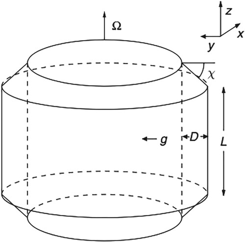
Whilst cylindrical coordinates would be an obvious choice for a coordinate system, by making the small gap approximation (i.e. $D\ll r_0$), the effects of curvature can be ignored and a Cartesian coordinate system used. The coordinate x is the Cartesian analogue of the azimuthal coordinate with $0\le x\le 2\pi$, y is the Cartesian analogue of the radial coordinate with $0\le y\le D$ and z is the axial coordinate with $-L/2\le z\le L/2.$ In this configuration, the annulus rotates with angular velocity $\mathit{\Omega }=\Omega \stackrel{\mathbf{ˆ}}{\mathit{z}}$, gravity is given by $\mathit{g}=g_0\stackrel{\mathbf{ˆ}}{\mathit{y}}$, and the imposed magnetic field is ${\mathit{B}}_{\mathbf{0}}=B_0\stackrel{\mathbf{ˆ}}{\mathit{x}}.$

In order to derive a set of equations governing the fluid flow in the Boussinesq approximation we begin with the vorticity equation including the Lorentz force term, given by (1) $\begin{array}{rl}& \frac{\mathrm{\partial }\mathit{Z}}{\mathrm{\partial }t}+\mathit{U}\cdot \mathrm{\nabla }\mathit{Z}-((2\mathit{\Omega }+\mathit{Z})\cdot \mathrm{\nabla })\mathit{U}=-\alpha \mathit{g}\times \mathrm{\nabla T}+\nu {\mathrm{\nabla }}^2\mathit{Z}+\frac{1}{{\mu }_0{\rho }_0}\mathrm{\nabla }\times \left((\mathit{B}\cdot \mathrm{\nabla })\mathit{B}\right),\end{array}$(1) where $\mathit{U}$ is the velocity, $\mathit{Z}=\mathrm{\nabla }\times \mathit{U}$ is the vorticity, $\mathit{B}$ is the magnetic field, and T is the temperature. Additionally, α is the coefficient of thermal expansion, ν is the viscosity, ${\rho }_0$ is the density and ${\mu }_0$ is the magnetic permeability. Similarly, we consider the curl of the induction equation given by (2) $\frac{\mathrm{\partial \nabla }\times \mathit{B}}{\mathrm{\partial }t}=\mathrm{\nabla }\times (\mathrm{\nabla }\times (\mathit{U}\times \mathit{B}))+\lambda {\mathrm{\nabla }}^2\mathrm{\nabla }\times \mathit{B},$(2) where λ is the magnetic diffusivity. The model is completed with a heat equation of the form (3) $\frac{\mathrm{\partial }T}{\mathrm{\partial }t}+(\mathit{U}\cdot \mathrm{\nabla })T=\kappa {\mathrm{\nabla }}^{2}T,$(3) where κ is the thermal diffusivity.

The basic state is given by $\mathit{U}={\mathit{U}}_{\mathbf{0}}=\mathbf{0}$, $\mathit{B}={\mathit{B}}_{\mathbf{0}}$, $T=T_0=\text{β}y$ and we perturb this by taking $\mathit{U}=\mathit{u}$, $\mathit{B}={\mathit{B}}_{\mathbf{0}}+\mathit{b}$, and $T=T_0+\theta$. In the rapidly rotating limit, we assume the sloped boundaries are nearly flat so $\chi \ll 1$ and the flow can be assumed to be quasi-geostrophic meaning the z-component of the velocity, $\mathit{u}$, is small compared with the x and y-components. This allows us to make the ansatz (4) $\mathit{u}\approx \mathrm{\nabla }\times \psi (x,y)\stackrel{\mathbf{ˆ}}{\mathit{z}}=\frac{\mathrm{\partial }\psi }{\mathrm{\partial }y}\stackrel{\mathbf{ˆ}}{\mathit{x}}-\frac{\mathrm{\partial }\psi }{\mathrm{\partial }x}\stackrel{\mathbf{ˆ}}{\mathit{y}},$(4) for the velocity where the vertical component, $u_z\ll u_x,u_y$. Following Hori et al. (2014), and for convenience, we choose an equivalent form for the magnetic field: (5) $\mathit{b}\approx \mathrm{\nabla }\times g(x,y)\stackrel{\mathbf{ˆ}}{\mathit{z}}=\frac{\mathrm{\partial }g}{\mathrm{\partial }y}\stackrel{\mathbf{ˆ}}{\mathit{x}}-\frac{\mathrm{\partial }g}{\mathrm{\partial }x}\stackrel{\mathbf{ˆ}}{\mathit{y}},$(5) where $b_z\ll b_x,b_y$. The fluid is contained within the annulus so we require a no-penetration condition on all boundaries. At the annular lids this condition depends on the angle, χ, made between the sloped walls and the horizontal so that (6) $\cos \left(\chi \right)u_z\mp \sin \left(\chi \right)u_y=0,$(6) on $z=\pm L/2$. Since $\chi \ll 1$ this becomes $u_z=\mp \chi \frac{\mathrm{\partial }\psi }{\mathrm{\partial }x}$ on $z=\pm L/2$. In our model we are interested in studying multiple jet solutions which are more readily produced through the addition of a bottom friction term in the equations. We add this term to $u_z$ to obtain (7) $u_z=\mp \chi \frac{\mathrm{\partial }\psi }{\mathrm{\partial }x}+U_E.$(7) Here $U_E$ is the optional Ekman suction term derived using a method by Greenspan (1968) and is given by $U_E=\mp D{\left(\frac{E}{2}\right)}^{1/2}\hat{\mathit{n}}\cdot \mathrm{\nabla }\times \left(\frac{1}{{|\hat{\mathit{n}}\cdot \hat{\mathit{z}}|}^{1/2}}(\hat{\mathit{n}}\times \mathit{u}+\mathit{u})\right)$ where $E=\nu /2\Omega D^2$ is the Ekman number. The Ekman suction term has been used in quasi-geostrophic models, for example Jones et al. (2003), Rotvig and Jones (2006) and Schaeffer and Cardin (2005), and is added to replicate the effects of an Ekman boundary layer when rigid top and bottom boundaries are implemented. This is absent in the case of stress-free top and bottom boundaries.

The perturbed forms given by (4(4) $\mathit{u}\approx \mathrm{\nabla }\times \psi (x,y)\stackrel{\mathbf{ˆ}}{\mathit{z}}=\frac{\mathrm{\partial }\psi }{\mathrm{\partial }y}\stackrel{\mathbf{ˆ}}{\mathit{x}}-\frac{\mathrm{\partial }\psi }{\mathrm{\partial }x}\stackrel{\mathbf{ˆ}}{\mathit{y}},$(4) )–(5(5) $\mathit{b}\approx \mathrm{\nabla }\times g(x,y)\stackrel{\mathbf{ˆ}}{\mathit{z}}=\frac{\mathrm{\partial }g}{\mathrm{\partial }y}\stackrel{\mathbf{ˆ}}{\mathit{x}}-\frac{\mathrm{\partial }g}{\mathrm{\partial }x}\stackrel{\mathbf{ˆ}}{\mathit{y}},$(5) ) are substituted into the vorticity equation (1(1) $\begin{array}{rl}& \frac{\mathrm{\partial }\mathit{Z}}{\mathrm{\partial }t}+\mathit{U}\cdot \mathrm{\nabla }\mathit{Z}-((2\mathit{\Omega }+\mathit{Z})\cdot \mathrm{\nabla })\mathit{U}=-\alpha \mathit{g}\times \mathrm{\nabla T}+\nu {\mathrm{\nabla }}^2\mathit{Z}+\frac{1}{{\mu }_0{\rho }_0}\mathrm{\nabla }\times \left((\mathit{B}\cdot \mathrm{\nabla })\mathit{B}\right),\end{array}$(1) ), the curl of the induction equation (2(2) $\frac{\mathrm{\partial \nabla }\times \mathit{B}}{\mathrm{\partial }t}=\mathrm{\nabla }\times (\mathrm{\nabla }\times (\mathit{U}\times \mathit{B}))+\lambda {\mathrm{\nabla }}^2\mathrm{\nabla }\times \mathit{B},$(2) ), and the heat equation (3(3) $\frac{\mathrm{\partial }T}{\mathrm{\partial }t}+(\mathit{U}\cdot \mathrm{\nabla })T=\kappa {\mathrm{\nabla }}^{2}T,$(3) ). The resulting vorticity equation is integrated over z and the boundary condition (7(7) $u_z=\mp \chi \frac{\mathrm{\partial }\psi }{\mathrm{\partial }x}+U_E.$(7) ) is used to eliminate the vertical velocity. The equations are non-dimensionalised using a lengthscale D, a viscous timescale $D^2/\nu$, a temperature scale $\text{β}D$, and a magnetic scale $B_0$. This gives the full nonlinear equations governing the fluid flow in our reduced 2D system as (8) $\begin{array}{rl}& \frac{\mathrm{\partial }{\mathrm{\nabla }}^2\psi }{\mathrm{\partial }t}+\frac{\mathrm{\partial }({\mathrm{\nabla }}^2\psi ,\psi )}{\mathrm{\partial }(x,y)}+B_f{\left|{\eta }^{\ast }\right|}^{1/2}{\mathrm{\nabla }}^2\psi -{\eta }^{\ast }\frac{\mathrm{\partial }\psi }{\mathrm{\partial }x}\\ =& \frac{\mathrm{Ra}}{\mathrm{Pr}}\frac{\mathrm{\partial }\theta }{\mathrm{\partial }x}+{\mathrm{\nabla }}^4\psi -\frac{Q}{\mathrm{Pm}}\frac{\mathrm{\partial }(g,{\mathrm{\nabla }}^{2}g)}{\mathrm{\partial }(x,y)}+\frac{Q}{\mathrm{Pm}}\frac{\mathrm{\partial }{\mathrm{\nabla }}^{2}g}{\mathrm{\partial }x},\end{array}$(8) (9) $\begin{array}{rl}& \frac{\mathrm{\partial }\theta }{\mathrm{\partial }t}-\frac{\mathrm{\partial }\psi }{\mathrm{\partial }x}+\frac{\mathrm{\partial }(\theta ,\psi )}{\mathrm{\partial }(x,y)}=\frac{1}{\mathrm{Pr}}{\mathrm{\nabla }}^2\theta ,\end{array}$(9) (10) $\begin{array}{rl}& \frac{\mathrm{\partial }{\mathrm{\nabla }}^{2}g}{\mathrm{\partial }t}=\frac{\mathrm{\partial }{\mathrm{\nabla }}^2\psi }{\mathrm{\partial }x}+{\mathrm{\nabla }}^2\frac{\mathrm{\partial }(\psi ,g)}{\mathrm{\partial }(x,y)}+\frac{1}{\mathrm{Pm}}{\mathrm{\nabla }}^{4}g,\end{array}$(10) where $\begin{array}{rl}{\eta }^{\ast }& =\frac{4\mathrm{\chi \Omega }{D}^3}{\mathrm{\nu L}},\mathrm{Ra}=\frac{g_0\alpha \text{β}{D}^4}{\mathrm{\nu \kappa }},\mathrm{Pr}=\frac{\nu }{\kappa },\\ Q& =\frac{B_0^2{D}^2}{{\rho }_0{\mu }_0\mathrm{\nu \lambda }},B_f={\left(\frac{D}{\mathrm{L\chi }}\right)}^{1/2},\mathrm{Pm}=\frac{\nu }{\lambda }.\end{array}$ In these equations, ${\eta }^{\ast }$ is a measure of the rotation rate (and is inversely related to the Ekman number, often used in spherical simulations, via $E=2\mathrm{D\chi }/L{\eta }^{\ast }$), Pr is the Prandtl number, Pm is the magnetic Prandtl number, Ra is the Rayleigh number, and Q is the Chandrasekhar number (measuring the input magnetic field strength). Additionally, the parameter $B_f$ controls the strength of the Ekman suction through a bottom friction term. Only when considering rigid top and bottom boundaries do we have $B_f\ne 0$. We shall also make use of the Elsasser number, defined as $\Lambda ={\eta }^{\ast }/Q.$ Our model is most relevant outside the tangent cylinder for a small but finite χ. As discussed by Rotvig and Jones (2006), the geometry of this model does not allow us to determine precisely where the annulus is situated within a sphere.

On the inner and outer annular walls, we assume stress-free, electrically conducting, constant temperature boundaries. Hence the boundary conditions are (11) $\begin{array}{rl}{u}_y=0& ⟹\frac{\mathrm{\partial }\psi }{\mathrm{\partial }x}=0,\end{array}$(11) (12) $\begin{array}{rl}\frac{\mathrm{\partial }{u}_x}{\mathrm{\partial }y}=0& ⟹\frac{{\mathrm{\partial }}^2\psi }{\mathrm{\partial }{y}^2}=0,\end{array}$(12) (13) $\begin{array}{r}\theta =0,\end{array}$(13) (14) $\begin{array}{rl}{b}_y=0& ⟹\frac{\mathrm{\partial }g}{\mathrm{\partial }x}=0,\end{array}$(14) on $y=0,1.$

Equations (8(8) $\begin{array}{rl}& \frac{\mathrm{\partial }{\mathrm{\nabla }}^2\psi }{\mathrm{\partial }t}+\frac{\mathrm{\partial }({\mathrm{\nabla }}^2\psi ,\psi )}{\mathrm{\partial }(x,y)}+B_f{\left|{\eta }^{\ast }\right|}^{1/2}{\mathrm{\nabla }}^2\psi -{\eta }^{\ast }\frac{\mathrm{\partial }\psi }{\mathrm{\partial }x}\\ =& \frac{\mathrm{Ra}}{\mathrm{Pr}}\frac{\mathrm{\partial }\theta }{\mathrm{\partial }x}+{\mathrm{\nabla }}^4\psi -\frac{Q}{\mathrm{Pm}}\frac{\mathrm{\partial }(g,{\mathrm{\nabla }}^{2}g)}{\mathrm{\partial }(x,y)}+\frac{Q}{\mathrm{Pm}}\frac{\mathrm{\partial }{\mathrm{\nabla }}^{2}g}{\mathrm{\partial }x},\end{array}$(8) )–(9(9) $\begin{array}{rl}& \frac{\mathrm{\partial }\theta }{\mathrm{\partial }t}-\frac{\mathrm{\partial }\psi }{\mathrm{\partial }x}+\frac{\mathrm{\partial }(\theta ,\psi )}{\mathrm{\partial }(x,y)}=\frac{1}{\mathrm{Pr}}{\mathrm{\nabla }}^2\theta ,\end{array}$(9) ), subject to conditions (11(11) $\begin{array}{rl}{u}_y=0& ⟹\frac{\mathrm{\partial }\psi }{\mathrm{\partial }x}=0,\end{array}$(11) )–(13(13) $\begin{array}{r}\theta =0,\end{array}$(13) ), have been solved numerically in the non-magnetic case by, for example, Rotvig and Jones (2006), Jones et al. (2003) and Teed et al. (2012). This work examined bursts of convection and multiple jets and found that the latter were more readily produced when rigid boundaries were implemented while the former were more common with stress-free boundaries. The non-magnetic equations have also been solved analytically in the linear case by Busse (1970) where, in the limit of rapid rotation, the (non-magnetic) critical Rayleigh number $R{a}_c^{\mathrm{HD}}$ is found to be (15) $R{a}_c^{\mathrm{HD}}=3{\left(\frac{{\eta }^{\ast }\mathrm{Pr}}{\sqrt{2}(1+\mathrm{Pr})}\right)}^{4/3}.$(15) Equations (8(8) $\begin{array}{rl}& \frac{\mathrm{\partial }{\mathrm{\nabla }}^2\psi }{\mathrm{\partial }t}+\frac{\mathrm{\partial }({\mathrm{\nabla }}^2\psi ,\psi )}{\mathrm{\partial }(x,y)}+B_f{\left|{\eta }^{\ast }\right|}^{1/2}{\mathrm{\nabla }}^2\psi -{\eta }^{\ast }\frac{\mathrm{\partial }\psi }{\mathrm{\partial }x}\\ =& \frac{\mathrm{Ra}}{\mathrm{Pr}}\frac{\mathrm{\partial }\theta }{\mathrm{\partial }x}+{\mathrm{\nabla }}^4\psi -\frac{Q}{\mathrm{Pm}}\frac{\mathrm{\partial }(g,{\mathrm{\nabla }}^{2}g)}{\mathrm{\partial }(x,y)}+\frac{Q}{\mathrm{Pm}}\frac{\mathrm{\partial }{\mathrm{\nabla }}^{2}g}{\mathrm{\partial }x},\end{array}$(8) )–(10(10) $\begin{array}{rl}& \frac{\mathrm{\partial }{\mathrm{\nabla }}^{2}g}{\mathrm{\partial }t}=\frac{\mathrm{\partial }{\mathrm{\nabla }}^2\psi }{\mathrm{\partial }x}+{\mathrm{\nabla }}^2\frac{\mathrm{\partial }(\psi ,g)}{\mathrm{\partial }(x,y)}+\frac{1}{\mathrm{Pm}}{\mathrm{\nabla }}^{4}g,\end{array}$(10) ) are identical to those derived by Hori et al. (2014) albeit with the addition of the bottom friction and nonlinear terms. The linear equations have been solved analytically for the magnetic case by Hori et al. (2014) where different limits for the Roberts number $q=\mathrm{Pm}/\mathrm{Pr}$ are considered, allowing solutions for the critical wavenumber and critical Rayleigh number. The magnetic critical Rayleigh number complicates matters since it is a function of Q and Pm. To ease comparison between different cases and parameter regimes explored, we measure the supercriticality in our model using the non-magnetic Rayleigh number given by equation (15(15) $R{a}_c^{\mathrm{HD}}=3{\left(\frac{{\eta }^{\ast }\mathrm{Pr}}{\sqrt{2}(1+\mathrm{Pr})}\right)}^{4/3}.$(15) ).

2.1. Numerical method

Equations (8(8) $\begin{array}{rl}& \frac{\mathrm{\partial }{\mathrm{\nabla }}^2\psi }{\mathrm{\partial }t}+\frac{\mathrm{\partial }({\mathrm{\nabla }}^2\psi ,\psi )}{\mathrm{\partial }(x,y)}+B_f{\left|{\eta }^{\ast }\right|}^{1/2}{\mathrm{\nabla }}^2\psi -{\eta }^{\ast }\frac{\mathrm{\partial }\psi }{\mathrm{\partial }x}\\ =& \frac{\mathrm{Ra}}{\mathrm{Pr}}\frac{\mathrm{\partial }\theta }{\mathrm{\partial }x}+{\mathrm{\nabla }}^4\psi -\frac{Q}{\mathrm{Pm}}\frac{\mathrm{\partial }(g,{\mathrm{\nabla }}^{2}g)}{\mathrm{\partial }(x,y)}+\frac{Q}{\mathrm{Pm}}\frac{\mathrm{\partial }{\mathrm{\nabla }}^{2}g}{\mathrm{\partial }x},\end{array}$(8) )–(10(10) $\begin{array}{rl}& \frac{\mathrm{\partial }{\mathrm{\nabla }}^{2}g}{\mathrm{\partial }t}=\frac{\mathrm{\partial }{\mathrm{\nabla }}^2\psi }{\mathrm{\partial }x}+{\mathrm{\nabla }}^2\frac{\mathrm{\partial }(\psi ,g)}{\mathrm{\partial }(x,y)}+\frac{1}{\mathrm{Pm}}{\mathrm{\nabla }}^{4}g,\end{array}$(10) ) are solved numerically by integrating forward in time using a collocation method (Boyd 2001) written in Fortran. We expand our fields ψ, θ and g using a Fourier expansion in x and a sine expansion in y, similar to the method used in previous non-magnetic simulations (Jones et al. 2003, Rotvig and Jones 2006, Teed et al. 2012). Therefore we set (16) $\begin{array}{rl}\psi (x,y,t)& =\frac{1}{2}\sum _{l=-(N_x-1)}^{N_x-1}\sum _{m=1}^{N_y-1}{\hat{\psi }}_{\mathrm{lm}}\left(t\right)\sin \left(\mathrm{m\pi y}\right){\mathrm{e}}^{-\mathrm{i}\mathrm{lx}\left(2\pi /L_x\right)},\end{array}$(16) (17) $\begin{array}{rl}\theta (x,y,t)& =\frac{1}{2}\sum _{l=-(N_x-1)}^{N_x-1}\sum _{m=1}^{N_y-1}{\hat{\theta }}_{\mathrm{lm}}\left(t\right)\sin \left(\mathrm{m\pi y}\right){\mathrm{e}}^{-\mathrm{i}\mathrm{lx}\left(2\pi /L_x\right)},\end{array}$(17) (18) $\begin{array}{rl}g(x,y,t)& =\frac{1}{2}\sum _{l=-(N_x-1)}^{N_x-1}\sum _{m=1}^{N_y-1}{\hat{g}}_{\mathrm{lm}}\left(t\right)\sin \left(\mathrm{m\pi y}\right){\mathrm{e}}^{-\mathrm{i}\mathrm{lx}\left(2\pi /L_x\right)},\end{array}$(18) where $N_x$ is the x resolution, $N_y$ is the y resolution and $L_x=2\pi$ is the length of the x domain. We apply a semi-implicit scheme by treating the linear terms implicitly using the Crank-Nicolson method and we treat the nonlinear terms explicitly using the second order Adams-Bashforth method. Simulations are initialised from a low amplitude mode or using the final state of a simulation in nearby parameter space, until a statistically steady state is reached. All simulations use the resolution $(N_x,N_y)=(256,128).$

2.2. Output parameters

When examining simulations we consider the total kinetic energy, the zonal energy and the magnetic energy defined by (19) $\begin{array}{rl}{E}_K& =\frac{1}{L_x}\int {\left(\mathrm{\nabla }\psi \right)}^2\mathrm{d}S=\frac{1}{8}\sum _{l=-(N_x-1)}^{N_x-1}\sum _{m=1}^{N_y-1}\mid {\hat{\psi }}_{\mathrm{lm}}{\mid }^2(l^2+m^2{\pi }^2),\end{array}$(19) (20) $\begin{array}{rl}{E}_Z& =\frac{1}{L_x}\int {\left({〈\mathrm{\nabla }\psi 〉}_x\right)}^2\mathrm{d}S=\frac{1}{8}\sum _{m=1}^{N_y-1}{m}^2{\pi }^2\mid {\hat{\psi }}_{0m}{\mid }^2,\end{array}$(20) (21) $\begin{array}{rl}{E}_M& =\frac{Q}{\mathrm{Pm}}\int {\left(\mathrm{\nabla }g\right)}^2\mathrm{d}S=\frac{Q}{8\mathrm{Pm}}\sum _{l=-(N_x-1)}^{N_x-1}\sum _{m=1}^{N_y-1}\mid {\hat{g}}_{\mathrm{lm}}{\mid }^2(l^2+m^2{\pi }^2),\end{array}$(21) respectively, where the x-average ${〈A〉}_x$ is defined as ${〈A〉}_x=\frac{1}{L_x}{\int }_0^{L_x}A\mathrm{d}x,$ for a scalar A. We will also be interested in the zonal flow $\overline{\mathbf{U}}$, which is defined as (22) $\mathbf{U}=U\hat{\mathbf{x}}={〈u_x〉}_x\hat{\mathbf{x}}=\frac{\mathrm{\partial }{〈\psi 〉}_x}{\mathrm{\partial }y}\hat{\mathbf{x}}⟹U=\frac{\mathrm{m\pi }}{2}{\hat{\psi }}_{0m}\cos \mathrm{m\pi y}.$(22) We wish to study the various forces in our system and to achieve this we consider the curl of each force given in the vorticity equation: $\underset{\mathrm{Inertia}}{\underbrace{\frac{\mathrm{\partial }{\mathrm{\nabla }}^2\psi }{\mathrm{\partial }t}+\frac{\mathrm{\partial }({\mathrm{\nabla }}^2\psi ,\psi )}{\mathrm{\partial }(x,y)}}}-\underset{\mathrm{Coriolis}}{\underbrace{{\eta }^{\ast }\frac{\mathrm{\partial }\psi }{\mathrm{\partial }x}}}+\underset{\mathrm{Bottom}\mathrm{friction}}{\underbrace{B_f{\left|{\eta }^{\ast }\right|}^{1/2}{\mathrm{\nabla }}^2\psi }}$ $=\underset{\mathrm{Buoyancy}}{\underbrace{\frac{\mathrm{Ra}}{\mathrm{Pr}}\frac{\mathrm{\partial }\theta }{\mathrm{\partial }x}}}+\underset{\mathrm{Viscosity}}{\underbrace{{\mathrm{\nabla }}^4\psi }}+\underset{\mathrm{Lorentz}}{\underbrace{\frac{Q}{\mathrm{Pm}}\frac{\mathrm{\partial }{\mathrm{\nabla }}^{2}g}{\mathrm{\partial }x}+\frac{Q}{\mathrm{Pm}}\frac{\mathrm{\partial }({\mathrm{\nabla }}^{2}g,g)}{\mathrm{\partial }(x,y)}}}.$ This approach, where the curl of forces have been used, has been examined previously by Teed and Dormy (2023) and Mason et al. (2022) in a spherical setting. We adopt this for convenience since our numerical scheme solves for the curl of the Navier-Stokes rather than the Navier-Stokes equation itself. We denote the curl of a force by $\mathit{C}$ and define $C^2=\frac{1}{L_x}\int {\mathit{C}}^2\mathrm{d}S=\frac{1}{L_x}\sum _{l=0}^{N_x}\sum _{m=1}^{N_y}{C}_{\mathrm{lm}}^2,$ allowing us to form a spectrum of the curl of each force in l and m, given by $C_{\mathrm{lm}}$. This gives the curl of each force as (23) $\begin{array}{rl}{C}_C^2& =\frac{{\eta }^{{\ast }^2}}{8}\sum _{l=-(N_x-1)}^{N_x-1}\sum _{m=1}^{N_y-1}{l}^2|{\hat{\psi }}_{\mathrm{lm}}{|}^2,\end{array}$(23) (24) $\begin{array}{rl}{C}_A^2& =\frac{R{a}^2}{8P{r}^2}\sum _{l=-(N_x-1)}^{N_x-1}\sum _{m=1}^{N_y-1}{l}^2|{\hat{\theta }}_{\mathrm{lm}}{|}^2,\end{array}$(24) (25) $\begin{array}{rl}{C}_V^2& =\frac{1}{8}\sum _{l=-(N_x-1)}^{N_x-1}\sum _{m=1}^{N_y-1}{(l^2+m^2{\pi }^2)}^4|{\hat{\psi }}_{\mathrm{lm}}{|}^2,\end{array}$(25) (26) $\begin{array}{rl}{C}_L^2& =\frac{Q^2}{2P{m}^2}\sum _{l=-(N_x-1)}^{N_x-1}\sum _{m=1}^{N_y-1}|A_{\mathrm{lm}}{|}^2,\end{array}$(26) (27) $\begin{array}{rl}{C}_I^2& =\frac{1}{2}\sum _{l=-(N_x-1)}^{N_x-1}\sum _{m=1}^{N_y-1}|B_{\mathrm{lm}}{|}^2,\end{array}$(27) (28) $\begin{array}{rl}{C}_{\mathrm{bf}}^2& =\frac{B_f^2{\eta }^{\ast }}{8}\sum _{l=-(N_x-1)}^{N_x-1}\sum _{m=1}^{N_y-1}{(l^2+m^2{\pi }^2)}^2|{\hat{\psi }}_{\mathrm{lm}}{|}^2,\end{array}$(28) where the subscripts C, A, V, L, I, and bf refer to the Coriolis, buoyancy, viscous, Lorentz, inertial, bottom friction forces, respectively. We denote the nonlinear term in the Lorentz force by $A_{\mathrm{lm}}$ and the nonlinear term in the inertial force by $B_{\mathrm{lm}}.$ We have neglected the time derivative in the inertial term and the x-derivative in the Lorentz term, as these are much smaller than the nonlinear terms. In our work we will consider the total curl of each force, found by summing over both l and m, although the expressions (23(23) $\begin{array}{rl}{C}_C^2& =\frac{{\eta }^{{\ast }^2}}{8}\sum _{l=-(N_x-1)}^{N_x-1}\sum _{m=1}^{N_y-1}{l}^2|{\hat{\psi }}_{\mathrm{lm}}{|}^2,\end{array}$(23) )–(28(28) $\begin{array}{rl}{C}_{\mathrm{bf}}^2& =\frac{B_f^2{\eta }^{\ast }}{8}\sum _{l=-(N_x-1)}^{N_x-1}\sum _{m=1}^{N_y-1}{(l^2+m^2{\pi }^2)}^2|{\hat{\psi }}_{\mathrm{lm}}{|}^2,\end{array}$(28) ) would also allow a study of the lengthscale dependence of each curl of force.

3. Results

We perform runs for both the non-magnetic and magnetic case. We start with the non-magnetic case to ensure we obtain the same results as previous studies and to discuss the main characteristics of a multiple jet solution. We then consider the effect of varying the magnetic field strength Q and the Rayleigh number Ra for particular choices of Pm and $B_f$. The main focus of this work is to examine the effects of a magnetic field on the multiple jets so, for simplicity, we do not vary ${\eta }^{\ast }$, leaving this to a future study. We fix ${\eta }^{\ast }=5\times {10}^5$ since a large rotation rate is needed for multiple jet solutions and previous work by Teed et al. (2012) have found multiple jets at this value. We fix Pr = 1 and consider Pm = 0.5 and Pm = 5 with ${10}^3\le Q\le {10}^5$ and $2\le \mathrm{Ra}/R{a}_c^{\mathrm{HD}}\le 10$. We briefly discuss $B_f=0$ for the non-magnetic case and then consider $B_f=0.5$ in both the non-magnetic and magnetic case.

Previous studies require two conditions to be satisfied for a solution to be described to admit “multiple jets”. First, the dominant (time-averaged) mode $\hat{m}$ of the l = 0 component should satisfy $\hat{m}\ge 3$. Second, the (time-averaged) ratio of zonal to kinetic energy should satisfy $E_Z/E_K>\mathrm{0.05.}$ We follow these criteria but with an additional condition. We also require the l = 0 mode to be the dominant azimuthal mode. This extra condition is added because the magnetic field is found to be capable of breaking the axisymmetry of the flow pattern, which is always axisymmetric in the non-magnetic case. We denote the number of jets found in a simulation by $M=\hat{m}+1$ meaning a “multiple jet” solution has at least 4 jets.

3.1. Non-magnetic case

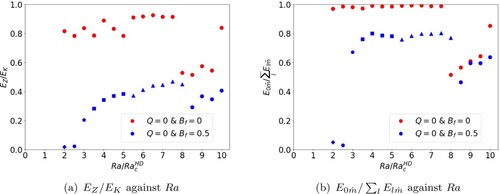
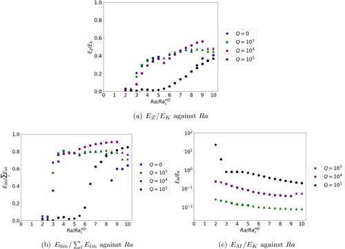
The non-magnetic case has been examined in great detail, where multiple jets are mainly found for $B_f\ne 0$ (Jones et al. 2003, Rotvig and Jones 2006, Teed et al. 2012). A few isolated cases of multiple jets have been found for $B_f=0$ in a small window of parameter space close to onset with a suitably large rotation rate (Jones et al. 2003). Figure 2(a) shows a plot of the ratio of zonal to kinetic energy against $\mathrm{Ra}/R{a}_c^{\mathrm{HD}}$, for different values of $B_f$ with the number of edges of each symbol indicating the time-averaged dominant mode $\hat{m}$. For $B_f=0$, we find strong zonal flows but no cases of multiple jets. Instead the dominant dynamics are quasi-periodic bursts of convection and zonal flow, in agreement with previous non-magnetic studies. At $B_f=0.5$, $E_Z/E_K$ is very small close to onset but builds as the driving increases (figure 2(a)). Multiple jet solutions are also obtained for this value of $B_f$ at the expense of a reduced zonal flow strength compared to the cases with $B_f=0$. This matches the trend found by Rotvig and Jones (2006) where $E_Z/E_K$ is large when $B_f=0$ and then decreases for larger $B_f.$ This is expected since $B_f$ increases the likelihood of multiple jets but weakens the zonal flow contribution through additional friction. A 6 jet solution is found at $\mathrm{Ra}/R{a}_c^{\mathrm{HD}}=3$, transitioning to 5 jets and then to 4 jets with increased driving before then dropping off to a solution without multiple jets. Each transition is associated with a reduction in the contribution of the zonal energy and highlights that the multiple jet phenomenon is restricted to a small window of Ra-space. Figure 2(b) provides further evidence of the nature of the solutions since the $(0,\hat{m})$ is shown to dominate over all other $(l,\hat{m})$ for solutions identified as having multiple jets. Therefore we can be satisfied these are azimuthally axisymmetric jets. The quantity plotted in figure 2(b) decreases when multiple jets are lost but remains large enough that l = 0 still dominates. This is similar to the case where $B_f=0$, where the ratio decreases at larger Ra but still remains large enough for $(0,\hat{m})$ to dominate.

Figure 2. Plots of energy against $\mathrm{Ra}/R{a}_c^{\mathrm{HD}}$ for $\mathrm{Pr}=1,$ ${\eta }^{\ast }=5\times {10}^5,$ and $Q=0$. Quantities have been globally averaged in space and time. The number of edges of each symbol represents the dominant time averaged mode $\hat{m}$. Plus symbols represent solutions with $\hat{m}\ge 7$ and circles represent solutions with $\hat{m}\le 2$. (a) $E_Z/E_K$ against Ra and (b) $E_{0\hat{m}}/\sum _l{E}_{l\hat{m}}$ against Ra. (Colour online)

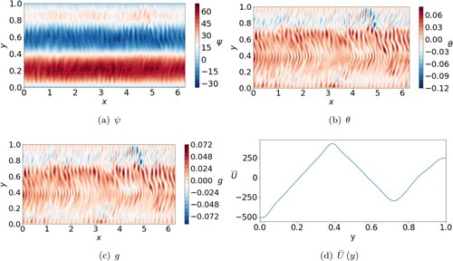
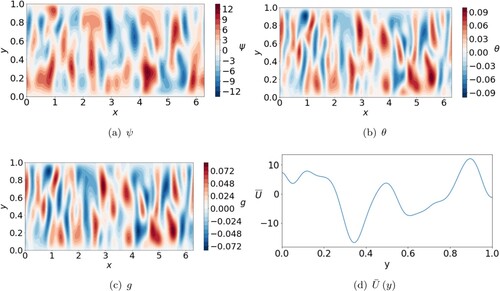
Typical solutions with and without multiple jets are shown in figures 3 and 4, respectively. A banded structure in ψ with 5 bands in the y-direction can be observed in figure 3(a), confirming an $\hat{m}=5$ dominant mode. The l = 0 component also dominates which is clear from the azimuthally axisymmetric nature of the flow. The zonal flow displays a multiple jet pattern, where a 6 jet solution is found. In θ we observe small structures and a negative temperature gradient in y attempting to erase the imposed basic state gradient. Solutions with multiple jets are quasi-steady once they have developed. Across all runs we present in this work, we never observe the jets change direction during a simulation. Once jets have developed, the dominant m mode does occasionally change for short periods of time as part of the dynamic evolution; this is also a feature of previous work by Rotvig and Jones (2006). 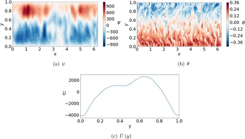However, for long periods of time the value of $\hat{m}$ (and, by association, the number of jets) remains unchanged from the time averaged values provided in our figures meaning there is no change in the number or direction of jets. This feature of the annulus model differs to beta-plane models where studies have shown the jets changing direction as the simulations move forward in time (Cope 2021). The case presented in figure 3 is typical of a multiple jet solution, matching previous work (Jones et al. 2003, Rotvig and Jones 2006, Teed et al. 2012). In figure 4 we no longer have multiple jets but, otherwise, the solution remains similar to that of figure 3. Axisymmetric flow and large $\overline{U}$ confirm the zonal nature of the solution despite the lack of multiple jets as expected from figure 2(b).

Figure 3. Snapshots of ψ, θ and zonal flow $\overline{U}$ for $\mathrm{Pr}=1,$ ${\eta }^{\ast }=5\times {10}^5$, $Q=0,$ $B_f=0.5,$ and $\mathrm{Ra}/R{a}_c^{\mathrm{HD}}=3.$ (a) ψ. (b) θ and (c) $\overline{U}\left(y\right)$. (Colour online)

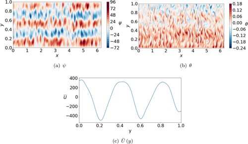
Figure 4. Snapshots of ψ, θ and zonal flow $\overline{U}$ for $\mathrm{Pr}=1,$ ${\eta }^{\ast }=5\times {10}^5$, $Q=0,$ $B_f=0.5,$ and $\mathrm{Ra}/R{a}_c^{\mathrm{HD}}=9.$ (a) ψ. (b) θ and (c) $\overline{U}\left(y\right)$. (Colour online)

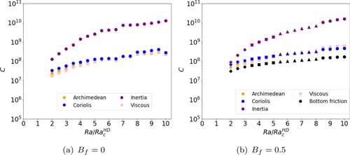
The curls of forces (figure 5) highlight the dominance of the inertial term in our solutions with a secondary Coriolis force typically in a balance with buoyancy and/or viscous forces. Figure 5(a) shows the global time-averaged curl of each force against $\mathrm{Ra}/R{a}_c^{\mathrm{HD}}$ for $B_f=0$. As we increase the driving, the inertial force increases at a faster rate than the other forces. The main difference between cases without (figure 5(b)) and with (figure 5(b)) bottom friction is increased contributions from the secondary forces in the latter. Indeed, the Coriolis and inertial terms are nearly in balance for low Ra when $B_f\ne 0$. These increased contributions, along with bottom friction, appear to be the catalyst for multiple jet solutions. An increase in the driving separates the inertial force from the secondary terms and solutions without multiple jets are preferred, in line with the $B_f=0$ cases.

Figure 5. Curl of each force against $\mathrm{Ra}/R{a}_c^{\mathrm{HD}}$ for $\mathrm{Pr}=1,$ ${\eta }^{\ast }=5\times {10}^5,$ and Q = 0. Quantities have been globally averaged in space and time. The number of edges of each symbol represents the dominant time averaged mode $\hat{m}$. Plus symbols represent solutions with $\hat{m}\ge 7$ and circles represent solutions with $\hat{m}\le 2$. (a) $B_f=0$ and (b) $B_f=0.5$. (Colour online)

3.2. Magnetic case

From previous work and earlier discussion it is clear that multiple jet solutions are more probable with a large rotation rate and bottom friction imposed. Our focus here will therefore be on cases with $B_f\ne 0$; in particular, in sections 3.2.2 and 3.2.3, we will study $B_f=0.5$ for two values of the magnetic Prandtl number: Pm = 0.5 and $\mathrm{Pm}=5.$ However, we first briefly examine multiple jets found when $B_f=0$ with a magnetic field imposed, discussing the main features and how this compares with the non-magnetic case.

3.2.1. No bottom friction

When $B_f=0$, multiple jets are possible at Pm = 0.5 and Pm = 5 close to onset (similar to results in the non-magnetic case by Jones et al. 2003). Figure 6 shows an example of such a solution. A similar flow structure is found to the multiple jets in the non-magnetic case with ψ featuring a banded structure and a dominant l = 0 and $\hat{m}=3$ mode. The structures in θ are small, g is very weak, and the zonal flow displays a multiple jet structure. In line with the non-magnetic case, very few cases of multiple jets are found for $B_f=0$. This is particularly true when the field strength is increased. Indeed, at large enough values of Q, no multiple jet solutions are found in the absence of bottom friction, even close to onset. For this reason the remainder of our results focus on $B_f\ne 0.$ We also note that, when $B_f=0$, cases with “bursts of convection” remain common in this magnetic case. These solutions are thus found in similar regions of parameter space to that in previous non-magnetic results (Jones et al. 2003, Rotvig and Jones 2006, Teed et al. 2012). Multiple jets and bursts of convection are never found together and bursting is uncommon at $B_f\ne 0$. We find no cases of bursting at $B_f=\mathrm{0.5.}$ Since our current study is focussed on multiple jet solutions, a thorough examination of the bursting solutions is left to a future study.

Figure 6. Snapshots of ψ, θ, g, and zonal flow $\overline{U}$ for $\mathrm{Pr}=1,$ ${\eta }^{\ast }=5\times {10}^5$, $Q={10}^3,$ $\mathrm{Pm}=0.5,$ $B_f=0,$ and $\mathrm{Ra}/R{a}_c^{\mathrm{HD}}=2.$ (a) ψ. (b) θ. (c) g and (d) $\overline{U}\left(y\right)$. (Colour online)

3.2.2. With bottom friction and Pm = 0.5

We now impose bottom friction, which is known to increase the likelihood of multiple jet solutions. We start by examining a magnetic Prandtl number Pm = 0.5, gradually increasing the magnetic field strength and driving to identify regions of parameter space where multiple jets are found.

Figure 7 highlights where multiple jet solutions are found and relative strengths of the zonal and magnetic energy for different values of Q and Ra. For $Q={10}^3$, multiple jets are readily found across Ra-space. A dip in $E_Z/E_K$ occurs at 5 times critical, associated with a reduction in the number of jets. For all Ra at $Q={10}^3$ the magnetic field does not play an important role as the ratio $E_M/E_K$ is small, meaning the zonal and total kinetic energy dominate. For this value of Q, rotation remains far more important than the magnetic field (since the Elsasser number, $\Lambda =Q/{\eta }^{\ast }\ll 1$) and the system essentially behaves as a magnetically adjusted version of the hydrodynamical solutions of section 3.1. It is notable that multiple jets persist for all values of Ra tested for $Q={10}^3$. This is in contrast to the Q = 0 case (cf. figure 3(a)) where multiple jets ceased at $\sim 8$ times critical. A magnetic field of weak enough strength is therefore conducive to multiple jet production at increased driving.

Figure 7. Plots of energy against $\mathrm{Ra}/R{a}_c^{\mathrm{HD}}$ for $\mathrm{Pr}=1,$ ${\eta }^{\ast }=5\times {10}^5$, Pm = 0.5, $B_f=0.5$ and varying Q. Quantities have been globally averaged in space and time. The number of edges of each symbol represents the dominant time averaged mode $\hat{m}.$ Plus symbols represent solutions with $\hat{m}\ge 7$ and circles represent solutions with $\hat{m}\le 2$. (a) $E_Z/E_K$ against Ra. (b) $E_{0\hat{m}}/\sum _l{E}_{l\hat{m}}$ against Ra and (c) $E_M/E_K$ against Ra. (Colour online)

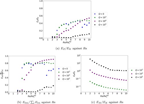
At $Q={10}^4$, multiple jet solutions emerge at low driving (albeit with small zonal energy) but soon transition to solutions with $\hat{m}<3$ as Ra is increased. This suggests there is an optimal value of field strength for production of multiple jets at larger Ra; for the current set of input parameters this optimal value of Q satisfies $0<Q<{10}^4$. The magnetic field has become important as the ratio of $E_M/E_K$ has increased significantly from $Q={10}^3$, reaching an $O\left(1\right)$ value for some values of Ra. It is clear from figure 7(b) that solutions for $Q={10}^3$ and $Q={10}^4$ (at least far from onset) are axisymmetric in nature with a strong zonal flow contribution, regardless of value of $\hat{m}$.

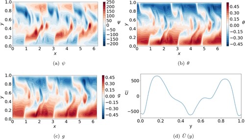
The snapshot plots of figure 8 are similar to equivalent plots of multiple jets for the non-magnetic case (cf. figure 3). Again, the flow is azimuthally axisymmetric (figure 8), the structures in θ and g are small (figure 8(b,c)) and the zonal flow shows a multiple jet pattern (figure 8(d)). The zonal flow is less symmetric than the equivalent non-magnetic case suggesting the magnetic field is capable of disturbing jet positioning locally at various times. The snapshots of figure 8 are typical of all multiple jet solutions found at $Q={10}^3$ and $Q={10}^4$, although, as we have seen, the precise number of jets is a function of the input control parameters.

Figure 8. Snapshots of ψ, θ, g and zonal flow $\overline{U}$ for $\mathrm{Pr}=1,$ ${\eta }^{\ast }=5\times {10}^5$, $Q={10}^3,$ $\mathrm{Pm}=0.5,$ $B_f=0.5,$ and $\mathrm{Ra}/R{a}_c^{\mathrm{HD}}=3.$ (a) ψ. (b) θ. (c) g and (d) $\overline{U}\left(y\right)$. (Colour online)

At $Q={10}^5$, the behaviour is strikingly different to that seen at other values of Q; this can first be noted through figure 7. The fraction of zonal energy is small for all values of Ra tested although a gradual increase in its value begins at $\sim 6$ times critical; nevertheless it remains small compared with its values when Q is lower. The value of $E_M/E_K$ is $O\left(1\right)$ or greater confirming that the magnetic field has now become dynamically important in the solutions. Figure 9 shows a typical solution for $Q={10}^5$ at low Ra. It is immediately clear that the zonal flow pattern has been lost at these input parameters. The solution in ψ is no longer azimuthally axisymmetric, structures are larger and the zonal flow is very weak.

Figure 9. Snapshots of ψ, θ, g and zonal flow $\overline{U}$ for $\mathrm{Pr}=1,$ ${\eta }^{\ast }=5\times {10}^5$, $Q={10}^5,$ $\mathrm{Pm}=0.5,$ $B_f=0.5,$ and $\mathrm{Ra}/R{a}_c^{\mathrm{HD}}=3.$ (a) ψ. (b) θ. (c) g and (d) $\overline{U}\left(y\right)$. (Colour online)

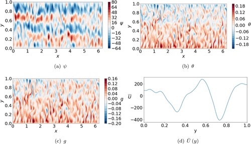
The value of $\hat{m}$ (given by the number of edges on the symbols in figure 7) suggests multiple jet solutions may be possible at $Q={10}^5$, once the driving is strong enough. However, figure 7(b) shows that l = 0 no longer dominates indicating that the axisymmetric nature of the solution has been destroyed. Figure 10 shows a typical solution for $Q={10}^5$ at larger Ra where $\hat{m}\ge 3$. The zonal flow displays a multiple jet structure but we no longer have azimuthally axisymmetric bands as shown in the snapshot for ψ (figure 10(a)). Instead we observe a 3-fold symmetry in the x-direction, confirming that the magnetic field is strong enough to break the axisymmetric nature of the flow. Through the snapshots of figure 10, it is clear that this is a different regime to both the multiple jet regimes at lower Q and the regimes at low Ra for $Q={10}^5$.

Figure 10. Snapshots of ψ, θ, g and zonal flow $\overline{U}$ for $\mathrm{Pr}=1,$ ${\eta }^{\ast }=5\times {10}^5$, $Q={10}^5,$ $\mathrm{Pm}=0.5,$ $B_f=0.5,$ and $\mathrm{Ra}/R{a}_c^{\mathrm{HD}}=9.$ (a) ψ. (b) θ. (c) g and (d) $\overline{U}\left(y\right)$. (Colour online)

The effect of magnetic field strength on the zonal flow can be summarised by figure 11 where two values of Ra are considered. It is clear in both cases that increasing the magnetic field strength dampens the zonal flow strength. We find strong zonal flows at $Q={10}^3$ which are almost completely suppressed at $Q={10}^5.$ This matches results by Tobias et al. (2007) where the effect of an imposed magnetic field on a β-plane was examined. For the larger value of Ra, the number of jets also reduces with increased field strength.

Figure 11. Zonal flow strength for increasing Q at two different values of $\mathrm{Ra}/R{a}_c^{\mathrm{HD}}$ with $\mathrm{Pr}=1,$ ${\eta }^{\ast }=5\times {10}^5$, Pm = 0.5, and $B_f=\mathrm{0.5.}$ The flow strength has been normalised by the largest value of $\overline{U}$ at each $\mathrm{Ra}/R{a}_c^{\mathrm{HD}}.$ (a) $\mathrm{Ra}/R{a}_c^{\mathrm{HD}}=4$ and (b) $\mathrm{Ra}/R{a}_c^{\mathrm{HD}}=10$. (Colour online)

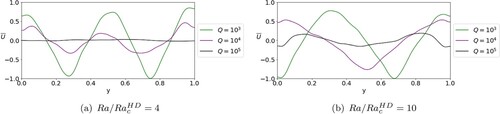
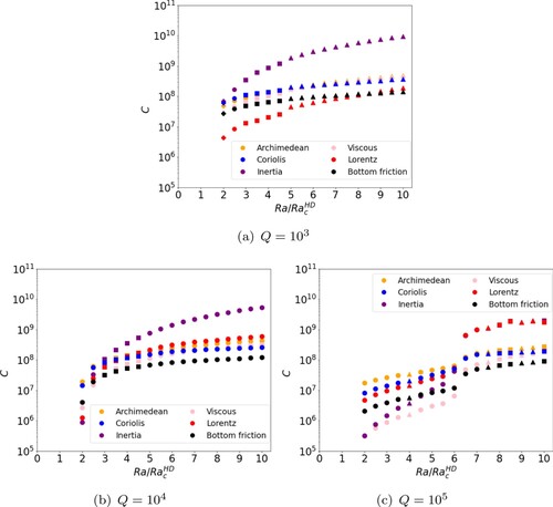
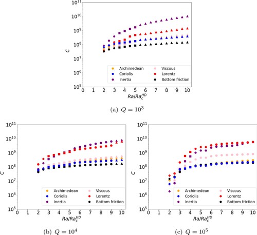
Figure 12 demonstrates different balances of (curls of) forces taking place at each Q tested. Figure 12(a), for $Q={10}^3$, is remarkably similar to the pattern observed in the non-magnetic case at $B_f=0.5$ (figure 5(b)) albeit with the addition of a weak Lorentz force. Very close to onset the inertial and Coriolis terms are nearly in balance and the buoyancy is also strong. As Ra is increased, all forces increase with the inertial term increasing at a faster rate and dominating throughout. In all cases the Lorentz term remains very weak but gradually increases relative to Coriolis, buoyancy and viscous terms. At the largest values of Ra tested, the Lorentz term begins to come into a secondary balance with the other forces. This highlights its role in preserving multiple jets at larger values of Ra (in contrast to the non-magnetic case where the force balance is otherwise equivalent). Figure 12(b) shows the (curls of) forces at $Q={10}^4$ where the hierarchy is similar to $Q={10}^3$, but with an increased Lorentz term for all Ra. Once supercriticality is high enough, a secondary balance between Lorentz, buoyancy, and Coriolis (MAC) emerges at moderate Ra where multiple jets occur. At larger Ra the hierarchy transitions such that the Lorentz term becomes the dominant secondary term; it is here that multiple jets are lost (though zonal flows remain). This indicates that, in contrast to $Q={10}^3$, the magnetic field can have a negative effect on multiple jet production, if its Lorentz force becomes strong enough. Nevertheless, with the Lorentz term remaining a secondary contribution below the inertia, zonal flows remain strong and prevalent. At $Q={10}^5$ (figure 12(c)) there is a stark change in the hierarchy of (curls of) forces. The dominant position of the inertial force is replaced with a quasi-MAC balance at low and moderate Ra. At $\mathrm{Ra}\approx 6.5R{a}_c^{\mathrm{HD}}$, a sudden change of regime occurs. The Coriolis and buoyancy terms increase entering a secondary balance with the viscous term, and the inertial and Lorentz terms increase drastically, forming the primary balance. This new balance coincides with the previously observed change in $\hat{m}$. There occurs a slight increase in $E_Z/E_K$ (figure 7(a)) as the inertial enters the primary balance but, ultimately, zonal flows and jets remain weak by the presence of the Lorentz term in the primary balance. This confirms that a strong enough magnetic field is able to suppress the development of zonal flows, as well as multiple jets.

Figure 12. Curl of each force against $\mathrm{Ra}/R{a}_c^{\mathrm{HD}}$ for $\mathrm{Pr}=1,$ ${\eta }^{\ast }=5\times {10}^5,$ Pm = 0.5 and varying Q. Quantities have been globally averaged in space and time. The number of edges of each symbol represents the dominant time averaged mode $\hat{m}$. Plus symbols represent solutions with $\hat{m}\ge 7$ and circles represent solutions with $\hat{m}\le 2$. (a) $Q={10}^3$. (b) $Q={10}^4$ and (c) $Q={10}^5$. (Colour online)

3.2.3. With bottom friction and Pm = 5

We now consider a larger value of Pm = 5, retaining bottom friction given by $B_f=0.5$. Figure 13(a), for Pm = 5, can be compared with figure 7(a), the equivalent for Pm = 0.5. The picture for low Q at Pm = 5 is very similar to that at Pm = 0.5. Again, at $Q={10}^3$, multiple jets persist for all Ra explored and at $Q={10}^4$ multiple jets appear at low and moderate Ra before being lost as the driving is increased. At $9.5R{a}_c^{\mathrm{HD}}$ and $10R{a}_c^{\mathrm{HD}}$ multiple jets reappear. In both cases, there is a drop in $E_Z/E_K$ coinciding with a reduction in the number of jets, with $Q={10}^3$ transitioning from a 5 jet to 4 jet solution and $Q={10}^4$ transitioning from multiple jets to a solution without multiple jets. This behaviour is similar to Pm = 0.5, where a drop in $E_Z/E_K$ occurred coinciding with a decrease in $\hat{m}$ although it is of note that the transition occurs at larger Ra compared to the Pm = 0.5 case. The solutions at $Q={10}^3$ are multiple jets, behaving similarly to those found in the non-magnetic case (figure 3) and magnetic case (figure 8). For both $Q={10}^3$ and $Q={10}^4$, $E_M/E_K$ is small and the solutions behave as magnetically adjusted hydrodynamical solutions with the magnetic field not having a clear discernible impact on the flow. At $Q={10}^5$, close to onset the behaviour at Pm = 5 is similar to Pm = 0.5. The ratio $E_Z/E_K$ is very small, $E_M/E_K$ is large and the magnetic field is now strong enough to suppress the development of zonal flows and multiple jets. Solutions at this value of Q are similar to those at Pm = 0.5 (e.g. figure 9) although the dominant azimuthal mode l has increased so the structures are smaller. As the driving is increased, the picture at Pm = 5 diverges from that at Pm = 0.5. The contribution of zonal energy increases steeply leading to the emergence of solutions with strong zonal flows and there is a gradual decrease in $E_M/E_K$. In this region of parameter space, solutions are similar to those found in previous non-magnetic and magnetic cases where zonal flows are strong but no multiple jets are found (e.g. figure 4). This is in stark contrast to the equivalent region of parameter space at $\mathrm{Pm}=0.5,$ where the magnetic field was able to suppress zonal flows and non-axisymmetric flow patterns emerged. Figure 13(b) confirms that, for Pm = 5, solutions with zonal flows and bands are produced at all values of Q provided driving is strong enough.

Figure 13. Plots of energy against $\mathrm{Ra}/R{a}_c^{\mathrm{HD}}$ for $\mathrm{Pr}=1,$ ${\eta }^{\ast }=5\times {10}^5$, Pm = 5, $B_f=0.5$ and varying Q. Quantities have been globally averaged in space and time. The number of edges of each symbol represents the dominant time averaged mode $\hat{m}.$ Plus symbols represent solutions with $\hat{m}\ge 7$ and circles represent solutions with $\hat{m}\le 2$. (a) $E_Z/E_K$ against Ra. (b) $E_{0\hat{m}}/\sum _l{E}_{l\hat{m}}$ against Ra and (c) $E_M/E_K$ against Ra. (Colour online)

The effect of increasing the magnetic field strength on the zonal flow strength can be summarised through figure 14. At $\mathrm{Ra}/R{a}_c^{\mathrm{HD}}=4$, the results are similar to Pm = 0.5 (cf. figure 11(a)), where increasing magnetic field strength suppresses zonal flows. However, at $\mathrm{Ra}/R{a}_c^{\mathrm{HD}}=9$, the increasing magnetic field does not suppress the zonal flow strength significantly but does reduce the jet number.

Figure 14. Zonal flow strength for increasing Q at two different values of $\mathrm{Ra}/R{a}_c^{\mathrm{HD}}$ with $\mathrm{Pr}=1,$ ${\eta }^{\ast }=5\times {10}^5$, Pm = 5, and $B_f=\mathrm{0.5.}$ (a) $\mathrm{Ra}/R{a}_c^{\mathrm{HD}}=4$ and (b) $\mathrm{Ra}/R{a}_c^{\mathrm{HD}}=9$. (Colour online)

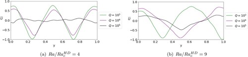
Figure 15, showing contributions from the curl of each force, gives a similar picture to the equivalent figure for Pm = 0.5 (cf. figure 12) but the contribution of the Lorentz term is boosted in each plot. At $Q={10}^3$, the inertial term is dominant throughout, similar to the Pm = 0.5 case, but with the Lorentz term being the leading secondary term. The inertial term remains an order of magnitude greater than all other terms and hence strong zonal flows and multiple jets exist. The plots for $Q={10}^4$ and $Q={10}^5$ each show the Lorentz term entering the primary balance. It is therefore evident that (compared with Pm = 0.5) at Pm = 5 the system requires a lower value of Q to transition from an inertially dominated regime to a balance between Lorentz and inertial terms. At Pm = 0.5 such a balance resulted in a loss of solutions with zonal flows (cf. figure 12(c)). Therefore it is somewhat surprising to find that the zonal flows (and in some cases, multiple jets) persist under this balance. Other than the boosted Lorentz force, the main difference in the hierarchy of curls of forces at the different values of Pm is a boosted viscous term. Unlike at Pm = 0.5, this strong secondary contribution preserves the axisymmetric nature of the solution so that zonal flows exist even when the Lorentz and inertial terms are in balance. Nevertheless, multiple jet solutions still remain elusive at large magnetic field strengths.

Figure 15. Curl of each force against $\mathrm{Ra}/R{a}_c^{\mathrm{HD}}$ for $\mathrm{Pr}=1,$ ${\eta }^{\ast }=5\times {10}^5$, Pm = 5 and varying Q. Quantities have been globally averaged in space and time. The number of edges of each symbol represents the dominant time averaged mode $\hat{m}$.Plus symbols represent solutions with $\hat{m}\ge 7$ and circles represent solutions with $\hat{m}\le 2$. (a) $Q={10}^3$. (b) $Q={10}^4$ and (c) $Q={10}^5$. (Colour online)

The MAC balance found at $Q={10}^5$ and low Ra in the Pm = 0.5 case is also found at Pm = 5 but over a much smaller window of Ra-space. It is worth noting that, for simplicity, our study has focussed on Rayleigh numbers normalised by the onset value for non-magnetic convection, $R{a}_c^{\mathrm{HD}}$. However, at Pm = 5, the Rayleigh numbers studied are more supercritical to the onset of magnetoconvection compared with Pm = 0.5 (since $R{a}_c^{\mathrm{MC}}(\mathrm{Pm}=5)<R{a}_c^{\mathrm{MC}}(\mathrm{Pm}=0.5)$). Further exploration at lower Ra may well extend this MAC regime in the Pm = 5 case. The stronger effective driving at Pm = 5 could also be enabling a zonal flow regime to emerge at larger Ra that is unseen in the lower Pm case.

3.3. Rhines scaling

By suggesting a balance between the inertial and Coriolis terms, the Rhines scaling theory (Rhines 1975) states that the lengthscale of the flow in the radial direction denoted by $L_R$, scales as $L_R\sim \sqrt{\frac{U}{{\eta }^{\ast }}},$ where U is a typical flow strength. It follows that the dominant wavenumber $m_r$ is given by (29) $m_r=c\sqrt{\frac{{\eta }^{\ast }}{U}},$(29) for some scaling factor, c, determined to best match simulation data. Rhines suggested that the convective (i.e. radial) speed should be used as the typical flow speed and some studies use this (e.g. Schneider and Liu 2009). Other studies, both in numerical simulations (Teed et al. 2012, Heimpel and Aurnou 2007) and in experimental work (Gillet et al. 2007), have instead defined U to be the zonal speed. In the non-magnetic case Jones et al. 2003 used the convective flow speed whereas Teed et al. 2012 examined both and found the zonal flow speed to fit best with the scaling theory.

In order to test our results against the theory, we define a convective flow speed and zonal flow speed as $\begin{array}{rl}{U}_C& =(max\left\{u_y\right\}-min\left\{u_y\right\})/2,\\ U_Z& =(max\left\{\overline{U}\right\}-min\left\{\overline{U}\right\})/2,\end{array}$ respectively. We wish to consider how our results match with the theory as well as which of $U_C$ and $U_Z$ best fits. The quantities $U_C$ and $U_Z$ are separately used in equation (29(29) $m_r=c\sqrt{\frac{{\eta }^{\ast }}{U}},$(29) ) to determine two values of $m_r$ for each simulation.

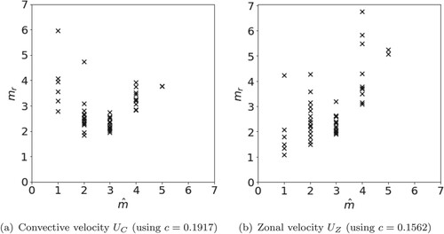
Figure 16 shows plots of the predicted wavenumber $m_r$ from the Rhines scaling theory against the dominant wavenumber $\hat{m}$ obtained from simulations using the convective velocity (figure 16(a)) and the zonal velocity (figure 16(b)), where the scaling factor c has been calculated to best match results obtained from simulations. For the Rhines scaling theory to hold, we expect a line of best fit where $m_r\approx \hat{m}.$ We have plotted non-magnetic results for both $B_f=0$ and $B_f=0.5$ and have plotted both values of Pm with $B_f=0.5$ for $Q={10}^3$ and $Q={10}^4,$ all for integer values of $\mathrm{Ra}/R{a}_c^{\mathrm{HD}}.$ We have excluded runs at $Q={10}^5$ and any runs where $E_Z/E_K\le 0.05$ because the theory does not hold for either the convective or zonal velocity. This is explained by the small zonal flows in these runs which result in unrealistically large values of $m_r$ in equation (29(29) $m_r=c\sqrt{\frac{{\eta }^{\ast }}{U}},$(29) ). When the convective velocity $U_C$ is used (figure 16(a)) the theory does not provide a good linear fit between $m_r$ and $\hat{m}.$ When the zonal velocity is used (figure 16(b)), a good linear fit exists between $m_r$ and $\hat{m}$ especially at lower $m_r.$ The theory arguably becomes slightly less accurate at larger values of $\hat{m}$ but overall when considering a linear fit between $m_r$ and $\hat{m}$, the zonal velocity provides the best fit. This matches the non-magnetic results of Teed et al. (2012) where they found the theory using the zonal flow speed to provide the best fit.

Figure 16. Plots of the predicted dominant $m_r$ from the scaling theory against the dominant mode $\hat{m}$ from simulations. (a) Convective velocity $U_C$ (using c = 0.1917) and (b) Zonal velocity $U_Z$ (using c = 0.1562).

For runs at $Q={10}^5$, we explored a different scaling by considering a balance between Coriolis and Lorentz terms due to the increased role of the magnetic field. This balance provides a scaling for the lengthscale of the flow as $L_{\mathrm{CL}}\sim \sqrt{\frac{Q{B}^2}{{\eta }^{\ast }\mathrm{UPm}}},$ where U is a typical flow strength and B is a typical magnetic field strength. This gives a dominant wavenumber $m_{\mathrm{CL}}$ as (30) $m_{\mathrm{CL}}=c\sqrt{\frac{{\eta }^{\ast }\mathrm{UPm}}{Q{B}^2}},$(30) for some scaling factor c. This was tested on our simulations for which a MAC balance occurs. However, we did not find a good linear fit between $\hat{m}$ in simulations and $m_{\mathrm{CL}}$ given by equation (30(30) $m_{\mathrm{CL}}=c\sqrt{\frac{{\eta }^{\ast }\mathrm{UPm}}{Q{B}^2}},$(30) ), indicating that this balance does not provide a prediction for the radial lengthscale.

4. Discussion

Our nonlinear simulations of convection in the Busse annulus model show good agreement with previous non-magnetic simulations (Jones et al. 2003, Rotvig and Jones 2006, Teed et al. 2012). In particular, we found that rigid top and bottom boundary conditions promoted the development of multiple jet solutions but also weakened the zonal flows. Many of the properties of the non-magnetic problem have been studied in detail previously but here we also examined the balances of the (curls of) forces of non-magnetic results. We found that a strong inertial term, with secondary contributions from the remaining terms, occurred for all runs. This is expected for zonal flows driven through the Reynolds stresses. For those simulations which displayed a multiple jet pattern of zonal flows (found typically at low driving with rigid boundaries), the inclusion of bottom friction provides an increased contribution from all secondary forces. Hence multiple jet structures appear to be facilitated in regimes where the inertial force is strong enough to produce zonal flows but secondary forces remain “only” 1-2 magnitudes weaker. This also provides an explanation as to why multiple jets are found in a small number of cases (at low Ra) where bottom friction is absent since weaker driving leads to weaker Reynolds stresses. Our non-magnetic results agreed well with the Rhines scaling when the zonal velocity was used, in agreement with previous work (Teed et al. 2012).

In this paper we extended the previous model by imposing an azimuthal magnetic field and examining the effect on multiple jet solutions as the magnetic field strength was varied. Several interesting conclusions can be drawn in the magnetic case. We found zonal flows and solutions with multiple jets are retained under the “correct” conditions. Typically, this requires a weak enough imposed field strength to either restrain the Lorentz force to be a secondary contributor or to maintain the inertial force in the primary balance alongside the Lorentz force. The remaining secondary forces, especially the viscous force, can also promote the retention of multiple jets. For multiple jets, relatively weak driving is also required (matching the non-magnetic case). Broadly speaking, an increased magnetic field strength reduces the number of jets and can, ultimately, completely suppress the development of multiple jets and zonal flows. However, a weak enough field can preserve multiple jets at larger driving, even compared to the non-magnetic case. The zonal flows of Mason et al. (2022) exhibit similar dependence on magnetic field strength. They find the magnetic field can increase the role of the zonal energy in the total kinetic energy (up to $\approx 30\mathrm{\%}$) but stronger imposed field suppresses the zonal flow. However, the flows in their spherical geometry appear to be driven by a thermal or magnetic wind whereas the importance of the inertial force in our work confirms that the flows are formed through Reynolds stresses. The flows in our (magnetic) work also form a far greater proportion of the kinetic energy budget (up to $\approx 50\mathrm{\%}$).

We found a MAC balance can be achieved in the annulus model. This was not necessarily expected since the model is geared towards generation of zonal flows through a strong inertial force (even at low driving) which must be absent in the MAC balance. The zonal flows (and multiple jets) are suppressed under such a balance. The effect of the magnetic Prandtl number, Pm, is subtle. Two values, an order of magnitude apart, were tested and we found the effect on zonal flow and multiple jet development to be minimal for the low values of imposed magnetic field (i.e. at $Q={10}^3$ and $Q={10}^4$ in our work). The patterns of a lowering of the number of jets and a reduction in the amplitude of the zonal energy as the driving is increased exist regardless of the value of Pm. At larger field strengths (i.e. at $Q={10}^5$ in our work), where the Elsasser number $\mathrm{\Lambda }=Q/{\eta }^{\ast }$ approaches its $O\left(1\right)$ optimal value for convective onset (Soward 1979, Hori et al. 2014), the available regimes depend greatly on Pm. At low driving, regimes are characterised by a MAC balance and weak zonal flow regardless of Pm but, with stronger driving, two different regimes are possible depending on Pm. Zonal flows, jets, and bands are replaced by non-axisymmetric solutions when the magnetic diffusion is large whereas the enhanced role of the viscous term when the magnetic diffusion is weak allows zonal flows to develop. Our results with large magnetic diffusion are in line with the spherical simulations of Mason et al. (2022), where imposing a strong enough magnetic field also suppresses zonal flows (although that work did not vary magnetic diffusion).

The Rhines scaling theory (using zonal flow speed) is unable to predict the number of jets if the imposed magnetic field is too large. The theory breaks down in regimes where the Lorentz force enters the primary balance with inertia since the theory is based on the assumption of a balance between only Coriolis and inertial forces.

Our work could be extended in various ways. For simplicity we have considered only a single value of the rotation rate. Although the value chosen was appropriate for the rapidly rotating regimes of planetary atmospheres and Earth's core, it should be varied to confirm existing results more widely. A second widely observed phenomenon of non-magnetic convection in the annulus model is the development of bursts of convection, interrupted by periods of strong zonal flows (Rotvig and Jones 2006, Jones et al. 2003, Teed et al. 2012). We have observed such behaviour in our magnetic model but have left its study for future work. The annulus model with an imposed magnetic field is known to admit various MHD waves (Hori et al. 2014) including the slow magnetic Rossby waves thought to be important in Earth's core and planetary atmospheres (Hori et al. 2018). The model may therefore be appropriate for studying the nonlinear behaviour of such waves in a simplified setting.

In our work we have chosen an imposed azimuthal (i.e. toroidal) magnetic field. Other options of field morphology are possible but we focussed on this configuration both for mathematical simplicity and because of the strong toroidal fields expected to be found in Earth's core and planetary atmospheres where magnetic field generation occurs. Recent work has shown that the multiple jets found on the surface of Jupiter extend roughly 3000 kilometres below the surface (Kaspi et al. 2023). Although we have used a simplified model, the parameter regime explored confirms jets found on Jupiter's surface, where a toroidal field is absent, will not penetrate into the metallic hydrogen region where the toroidal field is strong. The mechanism that creates multiple jets seen on Jupiter's surface is a feature of non-magnetic convection and models of the Jovian dynamo struggle to produce multiple jet structures in combination with a strong dipolar magnetic field (for e.g. Duarte et al. 2013, Jones 2014) without invoking the use of a stably-stratified layer (Gastine and Wicht 2021, Moore et al. 2022). We have shown here that it is possible to obtain multiple jets in the presence of a toroidal magnetic field without the need for a stably-stratified layer. However, whether this remains the case when the model is subject to a strong “poloidal-like” field (as appropriate for the molecular region of Jupiter) and under a wider parameter survey, remains to be seen. Nevertheless, magnetic fields may still have an observable effect on surface features even if they do not contribute to the generation of multiple jets (Hori et al. 2023). Our work also suggests zonal flows and multiple jets driven by Reynolds stresses may not be a feature of Earth's core where, like Jupiter, the expected balance of forces is “MAC”. However, a magnetic or thermal wind driven by, for example, spatially heterogeneous heat flux on the core-mantle boundary, provides an alternative zonal flow generation mechanism within Earth's core (Zhang and Gubbins 1996). The effects of an imposed magnetic field of different strengths on such a flow would need to be studied using a different set-up to our model, which assumes fixed temperature conditions. Finally, the magnetic field strengths found to preserve, and even promote, zonal flow and jet production in our model are likely not relevant to many known natural dynamos, which have strong dipolar fields under a “MAC balance”. However, they may be relevant to weak field spherical dynamos found numerically at low driving (Dormy et al. 2018) or dynamos of a non-dipolar nature.

Disclosure statement

No potential conflict of interest was reported by the author(s).

Additional information

Funding

This work was supported by EPSRC PhD Scholarship [EP/V519984/1].

References

- Aurnou, J., Calkins, M., Cheng, J., Julien, K., King, E., Nieves, D., Soderlund, K.M. and Stellmach, S., Rotating convective turbulence in Earth and planetary cores. Phys. Earth Planet. Inter. 2015, 246, 52–71.
- Boyd, J.P., Chebyshev and Fourier Spectral Methods, 2001 (Courier Corporation: New York).
- Brummell, N.H. and Hart, J., High Rayleigh number β-convection. Geophys. Astrophys. Fluid Dyn. 1993, 68, 85–114.
- Busse, F.H., Thermal instabilities in rapidly rotating systems. J. Fluid Mech. 1970, 44, 441–460.
- Busse, F.H., A simple model of convection in the Jovian atmosphere. Icarus 1976a, 29, 255–260.
- Busse, F.H., Generation of planetary magnetism by convection. Phys. Earth Planet. Inter. 1976b, 12, 350–358.
- Busse, F.H. and Finocchi, F., The onset of thermal convection in a rotating cylindrical annulus in the presence of a magnetic field. Phys. Earth Planet. Inter. 1993, 80, 13–23.
- Busse, F.H. and Or, A., Convection in a rotating cylindrical annulus: thermal Rossby waves. J. Fluid Mech. 1986, 166, 173–187.
- Cope, L. (2021). The dynamics of geophysical and astrophysical turbulence. Ph.D. Thesis.
- Dormy, E., Oruba, L. and Petitdemange, L., Three branches of dynamo action. Fluid Dyn. Res. 2018, 50, 011415.
- Duarte, L.D., Gastine, T. and Wicht, J., Anelastic dynamo models with variable electrical conductivity: an application to gas giants. Phys. Earth Planet. Inter. 2013, 222, 22–34.
- Duer, K., Galanti, E. and Kaspi, Y., Depth dependent dynamics explain the equatorial jet difference between Jupiter and Saturn. Geophys. Res. Lett. 2024, 51, e2023GL107354.
- Gastine, T. and Wicht, J., Stable stratification promotes multiple zonal jets in a turbulent Jovian dynamo model. Icarus 2021, 368, 114514.
- Gastine, T., Wicht, J., Duarte, L., Heimpel, M. and Becker, A., Explaining Jupiter's magnetic field and equatorial jet dynamics. Geophys. Res. Lett. 2014, 41, 5410–5419.
- Gillet, N., Brito, D., Jault, D. and Nataf, H., Experimental and numerical studies of convection in a rapidly rotating spherical shell. J. Fluid Mech. 2007, 580, 83–121.
- Greenspan, H.P., The Theory of Rotating Fluids, Vol. 327, 1968 (Cambridge University Press Cambridge).
- Heimpel, M. and Aurnou, J., Turbulent convection in rapidly rotating spherical shells: A model for equatorial and high latitude jets on Jupiter and Saturn. Icarus 2007, 187, 540–557.
- Heimpel, M., Aurnou, J. and Wicht, J., Simulation of equatorial and high-latitude jets on Jupiter in a deep convection model. Nature 2005, 438, 193–196.
- Heimpel, M., Gastine, T. and Wicht, J., Simulation of deep-seated zonal jets and shallow vortices in gas giant atmospheres. Nat. Geosci. 2016, 9, 19–23.
- Hori, K., Jones, C.A., Antuñano, A., Fletcher, L.N. and Tobias, S.M., Jupiter's cloud-level variability triggered by torsional oscillations in the interior. Nat. Astron. 2023, 7, 1–11.
- Hori, K., Takehiro, S.i. and Shimizu, H., Waves and linear stability of magnetoconvection in a rotating cylindrical annulus. Phys. Earth Planet. Inter. 2014, 236, 16–35.
- Hori, K., Teed, R. and Jones, C., The dynamics of magnetic Rossby waves in spherical dynamo simulations: a signature of strong-field dynamos? Phys. Earth Planet. Inter. 2018, 276, 68–85.
- Hutcheson, K.A. and Fearn, D.R., The nonlinear evolution of magnetic instabilities in a rapidly rotating annulus. J. Fluid Mech. 1995, 291, 343–368.
- Jones, C., Thermal and compositional convection in the outer core. Core Dyn. 2007, 8, 131–185.
- Jones, C., A dynamo model of Jupiter's magnetic field. Icarus 2014, 241, 148–159.
- Jones, C., Rotvig, J. and Abdulrahman, A., Multiple jets and zonal flow on Jupiter. Geophys. Res. Lett. 2003, 30, 1731.
- Kaspi, Y., Galanti, E., Park, R., Duer, K., Gavriel, N., Durante, D., Iess, L., Parisi, M., Buccino, D., Guillot, T., Stevenson, D.J. and Bolton, S.J., Observational evidence for cylindrically oriented zonal flows on Jupiter. Nat. Astron. 2023, 7, 1463–1472.
- Kurt, E., Busse, F.H. and Pesch, W., Hydromagnetic convection in a rotating annulus with an azimuthal magnetic field. Theor. Comput. Fluid Dyn. 2004, 18, 251–263.
- Mason, S.J., Guervilly, C. and Sarson, G.R., Magnetoconvection in a rotating spherical shell in the presence of a uniform axial magnetic field. Geophys. Astrophys. Fluid Dynam. 2022, 116, 458–498.
- Moore, K., Barik, A., Stanley, S., Stevenson, D., Nettelmann, N., Helled, R., Guillot, T., Militzer, B. and Bolton, S., Dynamo simulations of Jupiter's magnetic field: the role of stable stratification and a dilute core. Journal of Geophysical Research: Planets 2022, 127, e2022JE007479.
- Or, A. and Busse, F.H., Convection in a rotating cylindrical annulus. Part 2. Transitions to asymmetric and vacillating flow. J. Fluid Mech. 1987, 174, 313–326.
- Rhines, P.B., Waves and turbulence on a beta-plane. J. Fluid Mech. 1975, 69, 417–443.
- Rotvig, J. and Jones, C.A., Multiple jets and bursting in the rapidly rotating convecting two-dimensional annulus model with nearly plane-parallel boundaries. J. Fluid Mech. 2006, 567, 117–140.
- Schaeffer, N. and Cardin, P., Quasigeostrophic model of the instabilities of the Stewartson layer in flat and depth-varying containers. Phys. Fluids 2005, 17, 104111.
- Schnaubelt, M. and Busse, F.H., Convection in a rotating cylindrical annulus part 3. Vacillating and spatially modulated flows. J. Fluid Mech. 1992, 245, 155–173.
- Schneider, T. and Liu, J., Formation of jets and equatorial superrotation on Jupiter. J. Atmos. Sci. 2009, 66, 579–601.
- Soward, A., Convection driven dynamos. Phys. Earth Planet. Inter. 1979, 20, 134–151.
- Teed, R.J. and Dormy, E., Solenoidal force balances in numerical dynamos. J. Fluid Mech. 2023, 964, A26.
- Teed, R.J., Jones, C.A. and Hollerbach, R., On the necessary conditions for bursts of convection within the rapidly rotating cylindrical annulus. Phys. Fluids 2012, 24, 066604.
- Tobias, S.M., Diamond, P.H. and Hughes, D.W., β-plane magnetohydrodynamic turbulence in the solar tachocline. Astrophys. J. 2007, 667, L113.
- Wulff, P., Christensen, U.R., Dietrich, W. and Wicht, J., The effects of a stably stratified region with radially varying electrical conductivity on the formation of zonal winds on gas planets. Journal of Geophysical Research: Planets 2024, 129, e2023JE008042.
- Zhang, K. and Gubbins, D., Convection in a rotating spherical fluid shell with an inhomogeneous temperature boundary condition at finite Prandtl number. Phys. Fluids 1996, 8, 1141–1148.