Spatial statistical modelling of insurance risk: a spatial epidemiological approach to car insurance

ABSTRACT

Spatial models, such as the Besag, York and Mollie (BYM) model, have long been used in epidemiology and disease mapping. A common research question in these subjects is modelling the number of disease events per region; here the BYM models provides a holistic framework for both covariates and dependencies between regions. We use these tools to assess the relative insurance risk associated with the policyholders geographical location. A Bayesian modelling approach is presented and an elastic net is used to reduce the large number of possible geographic covariates. The final inference is performed using Integrated Nested Laplace Approximation. The model is applied to car insurance data from If P&C Insurance together with spatially referenced covariate data of high resolution, provided by Insightone. The entire analysis is performed using freely available R-packages. Including spatial dependence when modelling the number of claims significantly improves on the result obtained using ordinary generalised linear models. However, the support for adding a spatial component to the model for claims cost is weaker.

KEYWORDS:

• Bayesian hierarchical modelling
• geographical pricing
• integrated nested laplace approximation
• spatial modelling
• Besag–York–Mollie model

1. Introduction

An insurance contract is a policy that protects the policyholder against uncertain financial loss. Accurately predicting the risk associated with each policy allows the insurance company to differentiate its pricing between high and low risk policyholders.

The risk associated with a group of policies is described by the risk premium, $R_p$; defined as the total claims cost, C, divided by the total exposure, E, during a specified period of time, i.e. the total duration of active policies during that period (Ohlsson & Johansson 2010): (1) $R_p=\frac{C}{E}.$(1) The risk premium should cover the insurers expected cost for the policies. Although direct modelling of the risk premium is possible, it is common to split the modelling into two parts – modelling severity, S, and claims frequency, F, separately (Ohlsson & Johansson 2010, p. 34) (2) $R_p=\frac{C}{Y}\cdot \frac{Y}{E}=S\cdot F,$(2) where Y is the number of claims. The main reason for this separation is that claim frequency is usually much more stable than claim severity, allowing the frequency to be estimated with greater accuracy.

The frequency and severity are commonly modelled using multiplicative tariff models where the expected frequency (or severity) is given by the product of different rating factors (Ohlsson & Johansson 2010) (3) $\mathsf{E}\left(F_j\right)={\gamma }_0\cdot \prod _{k=1}^K{\gamma }_{k,j}.$(3) Here ${\gamma }_0$ is referred to as the base level and ${\gamma }_{k,j}$ can be thought of as relative risk for the $j\mathrm{th}$ policyholder with respect to the $k\mathrm{th}$ factor. Possible rating factors include age and gender¹ of the policyholder, characteristics of the insured object (e.g. value), and insurance history (i.e. past claims).

Geographic risk factors can be included by letting one of the rating factors, ${\gamma }_{G,i}$, represent the risks associated with the area, denoted by i, in which the jth policyholder lives. The geographic risk could be expected to depend on the area's demographic and socio-economic status; it would also be reasonable to expect the geographic risk to be similar among neighbouring areas. Already in the late 60's, prices were differentiated according to the size of the town or municipality in which the policyholder lived² . Recent advances in micro-geography, i.e. geographical location on a small scale, provides us with much richer, high resolution, spatial datasets that can be used to model geographic risk.

Here we wish to model the geographic risk in vehicle hull damage insurance data covering both claim frequency and severity. The available data (see Section 2) contains roughly 140 possible geographic covariates including demographic and socio-economic status at 13,831 division covering Stockholm's inner city and suburbs³. Given the large number of potential covariates elastic nets (Zou & Hastie 2005) were used for variable selection in the generalised linear models (GLMs); an approach previously suggested for variable selection when modelling non-geographic risk (Parodi 2012) and for spatial modelling of air pollution (Mercer et al. 2011).

Previous uses of geographical risk in non-life insurance (Assuncao et al. 2014) include modelling of loss ratios (claims cost divided by paid premium) in different postal code areas (Boskov & Verall 1994) and of claim frequency and severity over 440 regions of Germany (Gschlößl & Czado 2007).

The common approach in these, and other cases, is to use a generalised linear mixed model (GLMM) where the random effect is spatially structured; allowing it to capture geographical dependencies among neighbouring areas. The random effect is often modelled using a Besag, York and Mollie (BYM) model (Besag et al. 1991) with spatial dependence given by a Conditional Auto Regression (CAR) (Besag & Kooperberg 1995). These models are also popular in epidemiological and disease mapping applications (e.g. Ch. 6.2 in Waller & Carlin 2010, Blangiardo & Cameletti 2015).

Both Boskov & Verall (1994) and Gschlößl & Czado (2007) use single site Markov Chain Monte Carlo (MCMC) for Bayesian inference. For CAR models it has been demonstrated that single site updates lead to poor mixing for large dimensional models (Knorr-Held & Rue 2002). An alternative to MCMC based inference is approximate Bayesian inference using Integrated Nested Laplace Approximations (INLA) (Rue et al. 2009). For multiple models, including disease mapping with BYM models, INLA has been shown (Rue & Martino 2007, Rue et al. 2009) to yield almost instant inference in comparison with the time needed by MCMC to obtain decent accuracy (using e.g. OpenBUGS). Assuncao et al. (2014) has previously suggested using INLA to model claim frequency for a small (1833 regions) example data set.

The main contributions of this paper is illustrating how a combination of elastic nets for variable selection, BYM models for spatial dependence, and INLA for fast inference, can be used to efficiently model geographic risk in non-life insurance for large, complex datasets. To allow for operational use by insurance companies, our main empirical contribution is the use of publicly available statistical software (R, INLA, and glmnet; Friedman et al. 2010, R Development Core Team 2013, Lindgren & Rue 2015). INLA is able to fit models with spatial dependence structures to our 13,831 regions in minutes, and should be able to handle models with ${10}^5$–${10}^6$ geographic regions using a modern desktop computer (Rue et al. 2009). This allows us to handle dataset which are substantially larger and more complex than those previously studied.

2. Data

The data used here was obtained from a commercial provider (Insightone). The data illustrates both the advantages and limitations of commercially available high resolution geographic data.

The geographic data consists of area centroid coordinates and a neighbourhood structure; due to confidentiality Insightone does not provide exact area borders. The neighbourhood specification accounts for ‘natural’ obstacles, such as water, and conforms with the graph representation of neighbourhoods commonly used in CAR models (e.g. Ch. 6.1.2 in Blangiardo & Cameletti 2015). The division is depicted in Figure 1.

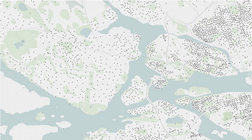
Figure 1. The division, into 13,831 areas, of Stockholm. Each point represents the centre of an area, the exact borders of the areas are not disclosed. Clearly the division is very granular in central Stockholm, but gets sparser in the outskirts of Stockholm.

In the division each of the areas are indexed – and associated to each area is a generous amount of underlying data such as gender distribution, age distribution and average income; giving roughly 140 possible geographic covariates. In addition to the external data, claims and insurance data for vehicle hull damage policies from the years 2011–2015 were provided. The choice of policies to study was motivated by the large amount of data and the relatively nice distribution of claims cost arising from this type of policies. Since the area borders are unknown each policy was associated with the closest area centroid using the address of that policyholder, $s_i$ – this corresponds to grouping the policies using a Voronoi tessellation based on the area centroids (Okabe et al. 2000) — and the aggregate number of claims, $Y_i$ and claims cost, $C_i$, in each area were computed.

3. Model

In line with the ordinary pricing models in insurance we assume that the geographic rating factors, ${\gamma }_{G,i}$, in each area can be modelled using a multiplicative model, see Equations (3(3) $\mathsf{E}\left(F_j\right)={\gamma }_0\cdot \prod _{k=1}^K{\gamma }_{k,j}.$(3) ) and (4(4) $Y_i\sim \mathsf{P}\mathsf{o}\left({\mathsf{E}}_{\mathsf{i}}\exp \mathsf{\left(}{\eta }_{\mathsf{i}}^{\mathsf{F}}\mathsf{\right)}\right)\mathsf{.}$(4) ). The geographic rating factors are then modelled using demographic and socio-economic variables (see Section 2) as well as neighbouring geographic rating factors. Using the aggregate number of claims and claims cost, this is in principle the same approach as in the ordinary tariff model, applied on the area-level. In principle this translates to assuming a GLM on the relative geographic rating factors ${\gamma }_{G,i}$ – letting the areas act as policyholders.

The first step of the modelling is to determine a suitable GLM model for the aggregated claim frequency and severity. This model will then be expanded to GLMM, Besag, and BYM models; allowing for spatial dependence through correlated random effects.

3.1. Aggregated claim frequency and severity

A standard model for claims frequency is to assume that the number of claims for a single policy follows a Poisson distribution (Ohlsson & Johansson 2010, p. 18). By assuming that policies are independent the number of claims on the aggregate level (i.e. areas) will also follow a Poisson distribution (Isham 2010). Thus, as in disease mapping (Waller & Carlin 2010), the number of events (claims), $Y_i$, in each area, i, are modelled using a Poisson distribution: (4) $Y_i\sim \mathsf{P}\mathsf{o}\left({\mathsf{E}}_{\mathsf{i}}\exp \mathsf{\left(}{\eta }_{\mathsf{i}}^{\mathsf{F}}\mathsf{\right)}\right)\mathsf{.}$(4) Here ${\eta }_i^F$ is the linear predictor of the GLM for claims frequency and $E_i$ is the exposure, i.e. total duration of policies, in area i. The areas will likely be inhomogeneous with respect to demography and socio-economic status. While this is preferable for geographical analysis of the data, some of the variation in risk between areas can be explained by the ordinary tariff. This can be taken into account in the measure of exposure. Thus, the raw exposure, $E_i$, is replaced by a weighted exposure, $E_i^{\ast }$, when modelling claim counts in area i.

The weighting is computed according to the composition of policyholders in each area and their rating factors. This method of obtaining a weighted exposure, $E_i^{\ast }$, compares to the weighted population (a.k.a. population at risk) used in disease mapping; where the distribution of e.g. age and gender in each area is accounted for in $E_i^{\ast }$, as discussed by Blangiardo & Cameletti (2015, p. 179) and Papoila et al. (2014, p. 1).

Although the number of claims is taken as response variable, the expected frequency, $F_i$, can always be found as (5) $\mathsf{E}\left[F_i|{\eta }_i^F\right]=\frac{1}{E_i^{\ast }}\mathsf{E}\left[Y_i|{\eta }_i^F\right]=\frac{1}{E_i^{\ast }}{E}_i^{\ast }\exp \left({\eta }_i^F\right)=\exp \left({\eta }_i^F\right),$(5) using Equations (4(4) $Y_i\sim \mathsf{P}\mathsf{o}\left({\mathsf{E}}_{\mathsf{i}}\exp \mathsf{\left(}{\eta }_{\mathsf{i}}^{\mathsf{F}}\mathsf{\right)}\right)\mathsf{.}$(4) ) and (2(2) $R_p=\frac{C}{Y}\cdot \frac{Y}{E}=S\cdot F,$(2) ).

As in Gschlößl & Czado (2007) the aggregate claims cost, $C_i$, in each area is modelled conditioned on the number of claims, $Y_i$. For claims cost the gamma distribution has become more or less the standard option in modelling (Ohlsson & Johansson 2010, p. 20). For the aggregate claims cost the use of a gamma distribution can be motivated by the addition over the given number of claims. We have (6) $C_i|Y_i=y_i\sim \mathrm{\Gamma }\left(y_{i}a,a\exp (-{\eta }_i^C)\right),$(6) with $\mathsf{E}[C_i|Y_i=y_i]=y_i\exp \left({\eta }_i^C\right)$ and $\mathsf{V}[C_i|Y_i=y_i]=\left(y_i/a\right)\exp \left(2{\eta }_i^C\right)$ and ${\eta }_i^C$ is the linear predictor for claims severity. If one is interested in the severity rather than the total claims cost, the scaling properties of the Gamma distribution yields (7) $\left.\frac{C_i}{Y_i}\right|Y_i=y_i\sim \mathrm{\Gamma }\left(y_{i}a,y_{i}a\exp (-{\eta }_i^C)\right)$(7) which implies that $\mathsf{E}[C_i/Y_i|Y_i=y_i]=\exp \left({\eta }_i^C\right)$.

The GLM for frequency and severity is now completed by assuming a linear model for η (suppressing the ^{${}^{F,C}$}-superscripts), (8) ${\eta }_i={\beta }_0+{\mathit{z}}_i\mathit{\beta },$(8) where ${\mathit{z}}_i$ is a (suitable) collection of underlying covariates in each area. Adding an individual level random effects to Equation (8(8) ${\eta }_i={\beta }_0+{\mathit{z}}_i\mathit{\beta },$(8) ) gives a GLMM, (9) ${\eta }_i={\beta }_0+{\mathit{z}}_i\mathit{\beta }+v_i,$(9) where the added i.i.d. Gaussian noise, $v_i$, accounts for moderate over-dispersion in the observations (Harrison 2014).

3.2. Modelling the spatial dependence

To allow for spatial dependence we instead add a structured random effect to the the linear predictor in Equation (8(8) ${\eta }_i={\beta }_0+{\mathit{z}}_i\mathit{\beta },$(8) ), resulting in a Besag model, (10) ${\eta }_i={\beta }_0+{\mathit{z}}_i\mathit{\beta }+u_i.$(10) Here $u_i$ is modelled using a CAR(1)-field (Besag & Kooperberg 1995).

Given a neighbourhood graph (see Figure 2 for an example) the CAR(1) model assumes that the value in one area is related to the values in neighbouring areas (i.e. areas that share a common border) through a conditional Gaussian distribution: (11) $u_i|\{u_j:j\in {\mathcal{N}}_i\}\sim \mathsf{N}\left(\frac{1}{|{\mathcal{N}}_i|}\sum _{j\in {\mathcal{N}}_i}{u}_j,\frac{1}{{\psi }_1|{\mathcal{N}}_i|}\right),$(11) where ${\mathcal{N}}_i$ is the set of neighbours to area i and ${\psi }_1$ is a precision parameter. The CAR(1) model corresponds to a multivariate Gaussian model for $\mathit{u}=\{u_i{\}}_i$ (Besag & Kooperberg 1995, Rue & Held 2005), (12) $\begin{array}{rl}\mathit{u}& \sim \mathsf{N}\left(\mathbf{0},{\psi }_1^{-1}{\mathit{Q}}^{-1}\right){\mathit{Q}}_{ij}=\left\{\begin{array}{ll}|{\mathcal{N}}_i|,& \mathrm{if}i=j,\\ -1,& \mathrm{if}j\in {\mathcal{N}}_i,\\ 0,& \mathrm{otherwise}.\end{array}\right.\end{array}$(12) Here, the resulting precision matrix (inverse covariance matrix) is sparse resulting in a Gaussian Markov Random Field (GMRF) allowing us to use INLA for fast approximate Bayesian inference (Rue et al. 2009, Lindgren & Rue 2015).

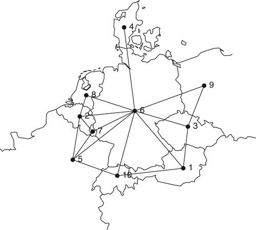
Figure 2. Map illustrating the duality between neighbourhood graph and spatial areas. All areas are represented by centroid coordinates and vertices connected by an edge indicate neighbours, i.e. areas that share a common border. For the data used in this paper only the neighbourhood structure (graph) is known since the area borders are confidential.

Combining the random effects in Equations (9(9) ${\eta }_i={\beta }_0+{\mathit{z}}_i\mathit{\beta }+v_i,$(9) ) and (10(10) ${\eta }_i={\beta }_0+{\mathit{z}}_i\mathit{\beta }+u_i.$(10) ) gives the BYM model (Besag et al. 1991), (13) ${\eta }_i={\beta }_0+{\mathit{z}}_i\mathit{\beta }+u_i+v_i.$(13) where $u_i$ is a CAR(1)-field and $v_i$ is i.i.d. Gaussian noise. As in the GLMM the i.i.d. noise accounts for moderate over-dispersion in the observations which could also be modelled using a Besag model with negative binomial observations.

3.3. Model and inference

The model for both claim frequency and severity can be summarised as a GLMM, using either a Poisson or gamma distribution for the observations and with the spatial dependence among areas captured using a BYM model. For the frequency, negative binomial observations are considered as an alternative to handle over-dispersion. Since the i.i.d. Gaussian noise in the BYM model accounts for moderate over-dispersion (Harrison 2014), negative binomial observations are only feasible in combination with a Besag model for spatial dependence (combining negative binomial observations with a BYM model leads to identifiability issues).

If $\pi \left(y_i|{\eta }_i\right)$ denotes the observation likelihood (Poisson, negative binomial, or gamma) for the $i\mathrm{th}$ observation given the linear predictor ${\eta }_i$, then the complete Bayesian hierarchical model is (14a) $\begin{array}{rl}{y}_i|{\eta }_i& \sim \pi \left(y_i|{\eta }_i\right),\end{array}$(14a) (14b) $\begin{array}{rl}{\eta }_i& ={\beta }_0+{\mathit{z}}_i\mathit{\beta }+u_i+v_i\end{array}$(14b) (14c) $\begin{array}{rl}\mathit{u}|{\psi }_1& \sim \mathsf{N}\left(\mathbf{0},{\psi }_1^{-1}{\mathit{Q}}^{-1}\right),\end{array}$(14c) (14d) $\begin{array}{rl}{v}_i|{\psi }_2& \sim \mathsf{N}(0,{\psi }_2^{-1}),\end{array}$(14d) (14e) $\begin{array}{rl}\mathit{\psi }& \sim \pi \left(\mathit{\psi }\right).\end{array}$(14e) The spatial effect (if any) is modelled through $\mathit{u}$ while the unstructured effects, $\mathit{v}$, models additional random variation, unexplained by geographical location. The larger the effect of $\mathit{v}$, compared to $\mathit{u}$, is in the model, the less exchange of information between areas is allowed. The precision (inverse variance) of $\mathit{u}$ and $\mathit{v}$ – i.e. the relative strengths of the structured and unstructured effects – are controlled by the two hyper-parameters ${\psi }_1$ and ${\psi }_2$, respectively. Two common choice for the priors for $\mathit{\psi }$ are either independent gamma distributions (Ch. 6 in Gschlößl & Czado 2007, Waller & Carlin 2010, Blangiardo & Cameletti 2015) or the recently introduced principled (PC) priors (Simpson et al. 2017, Fuglstad et al. 2018). Here we use both the default uninformative priors in INLA, ${\psi }_i\sim \mathrm{\Gamma }(1,5\cdot {10}^{-4})$ (Lindgren & Rue 2015) and the default INLA PC-priors (Bakka et al. 2018).

A final step before fitting the model is to determine which of the roughly 140 possible geographic covariates to include in ${\mathit{z}}_i$. A suitable set of candidate covariates were first selected using elastic net for the regular GLM, Equation (8(8) ${\eta }_i={\beta }_0+{\mathit{z}}_i\mathit{\beta },$(8) ), as described in Section 3.4. Then the model in Equation (14a(14a) $\begin{array}{rl}{y}_i|{\eta }_i& \sim \pi \left(y_i|{\eta }_i\right),\end{array}$(14a) ) was fitted in R, using the INLA-package (http://www.r-inla.org, Lindgren & Rue 2015), and the number of covariates where further reduced using posteriors, $p\left(\beta |\mathit{y}\right)$, and deviance information criterion (DIC) values provided by INLA, see Section 4

3.4. Selecting covariates

Including all the possible covariates in the model is likely to result in an over-fitted model that is hard to interpret. Additionally, many of the covariates are highly correlated, with the potential of causing numerical and identifiability issues when fitting the model. A first step is therefore to extract a suitable subset of candidate covariates for use in the full model, Equation (14a(14a) $\begin{array}{rl}{y}_i|{\eta }_i& \sim \pi \left(y_i|{\eta }_i\right),\end{array}$(14a) ). The idea, inspired by the two-step procedure used by Mercer et al. (2011), is to initially consider frequency and severity as pure GLMs, i.e. excluding all spatial and unstructured effects, and choose as few parameters as possible while retaining as much predictive quality as possible. Completing this in an algorithmic or at least structured fashion is desirable.

An effective algorithm for this purpose is the elastic net (Zou & Hastie 2005). A ready-to-use implementation of the algorithm is available in the R-package glmnet (Friedman et al. 2010). Consider a GLM, and let $l(Y_i,{\beta }_0+\mathit{\beta }{\mathit{z}}_i)$ denote the negative log-likelihood for observation i. The elastic net then solves the following convex optimisation problem (15) $\underset{{\beta }_0,\mathit{\beta }}{min}\frac{1}{N}\sum _{i=1}^{N}l(Y_i,{\beta }_0+{\mathit{z}}_i\mathit{\beta })+\lambda \left[(1-\alpha )||\mathit{\beta }|{|}_2^2/2+\alpha ||\mathit{\beta }|{|}_1\right],$(15) over a grid of values of λ, where $||\cdot |{|}_p$ denotes the $L_p$- norm.

The elastic net extends on the standard LASSO (Hastie et al. 2001, Ch. 3.4.3) by allowing a combination of $L_1$ and $L_2$ penalties in Equation (15(15) $\underset{{\beta }_0,\mathit{\beta }}{min}\frac{1}{N}\sum _{i=1}^{N}l(Y_i,{\beta }_0+{\mathit{z}}_i\mathit{\beta })+\lambda \left[(1-\alpha )||\mathit{\beta }|{|}_2^2/2+\alpha ||\mathit{\beta }|{|}_1\right],$(15) ), allowing the elastic net to better handle correlated covariates. It is known that $\alpha =0$ shrinks the coefficients of correlated covariates towards each other while $\alpha =1$ tends to pick one of them and discard the others (Friedman et al. 2010). The idea of the elastic net is to mix these properties, i.e. choosing $0<\alpha <1$. If predictors are correlated in groups, as is highly likely for our demographic and socio-economic variables, an α around 0.5 tends to select the groups in or out together. The tuning parameter λ controls shrinkage and thus the number of selected covariates. To obtain an optimal choice of λ glmnet applies a K-fold cross-validation.

Unfortunately the glmnet-package does not support gamma distributed observations, obstructing the direct implementation in the case of the claims cost model. Our approach was to model claims cost as log-normally distributed for the initial variable selection, since glmnet supports normal observations. The idea is that the algorithm should still (roughly) give the same suggestions of best covariates to include, even if another observational distribution is assumed. Note that the models which include spatial random effects (Besag and BYM) are expected to need fewer covariates compared to the GLM model, thus the elastic net is only used as a first step in the variable selection. Although elastic net penalties can be implemented for gamma distributed observations the log-normal approach allows us to use standard software, increasing the reproducibility of the method and results.

4. Results

For both claims frequency and claims severity models using four different linear predictors, see Table 1, are fitted to the available data. All of the models share the general form specified in Equation (14a(14a) $\begin{array}{rl}{y}_i|{\eta }_i& \sim \pi \left(y_i|{\eta }_i\right),\end{array}$(14a) ), but differ in the combination of unstructured, $v_i$, and spatially structured, $u_i$, random effects included in the linear predictor, η. For the claims frequency, models using both Poisson and negative binomial observations as well as two types of priors are also considered (Table 1).

Table 1. The four linear predictors as well as the different priors and observation models used.

Model name	Linear predictor	Defined in
GLM	${\eta }_i={\beta }_0+{\mathit{z}}_i\mathit{\beta }$	Equation (8(8) ${\eta }_i={\beta }_0+{\mathit{z}}_i\mathit{\beta },$(8) )
GLMM	${\eta }_i={\beta }_0+{\mathit{z}}_i\mathit{\beta }+v_i$	Equation (9(9) ${\eta }_i={\beta }_0+{\mathit{z}}_i\mathit{\beta }+v_i,$(9) )
Besag	${\eta }_i={\beta }_0+{\mathit{z}}_i\mathit{\beta }+u_i$	Equation (10(10) ${\eta }_i={\beta }_0+{\mathit{z}}_i\mathit{\beta }+u_i.$(10) )
BYM	${\eta }_i={\beta }_0+{\mathit{z}}_i\mathit{\beta }+u_i+v_i$	Equation (13(13) ${\eta }_i={\beta }_0+{\mathit{z}}_i\mathit{\beta }+u_i+v_i.$(13) )
Besag – Nbin	As Besag but using a negative binomial observations; only used for claims frequency.
BYM – PC	As BYM but using principled priors instead of uninformative Γ-priors; only used for claims frequency.

The available data consists of 13,831 areas, to allow for model evaluation the areas are randomly split into a modelling set ($90\mathrm{\%}$ of the areas) and a validation set ($10\mathrm{\%}$ of the areas). The modelling set is used for covariate selection, parameter estimation, and prediction of the validation set.

4.1. Using elastic net to select covariates

The first step in the modelling is to apply the elastic net to the regular GLM model, Equation (8(8) ${\eta }_i={\beta }_0+{\mathit{z}}_i\mathit{\beta },$(8) ); with the aim of extracting a (small) set of candidate geographic covariates from the roughly 140 potential covariates.

The cross-validation results from applying the elastic net algorithm with $\alpha =0.5$ and different penalties, λ, are displayed in Figure 3. The recommended approach (Hastie et al. 2001, Ch. 7.10) is to find the penalty, ${\lambda }_{\min }$, that minimises the cross-validation error and then pick the smallest λ such that the resulting error is within one standard error of the minimal error; i.e. pick the smallest model such that the error is not ‘statistically different’ from the minimal error.

Figure 3. Validation error with 95% confidence bounds from a 10-fold cross-validation using the elastic net algorithm on (a) frequency and (b) severity. The two vertical lines mark the penalty, ${\lambda }_{\min }$, giving the minimal error and the penalty giving an error within one standard error of the minimal error. (a) Frequency and (b) Severity.

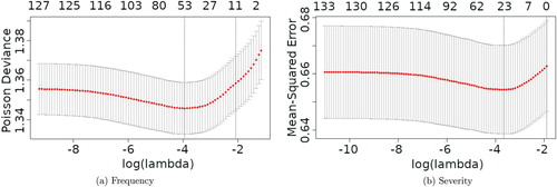
For the frequency data this approach works well and results in the selection of 16 candidate covariates. For the severity data the large uncertainty in the cross-validation error (Figure 3(b)) causes the one standard error approach to select no covariates. The reasonable choice here is to simply accept the 31 candidate covariates obtained for ${\lambda }_{\min }$.

The number of covariates might be further reduced when fitting the model without penalisation term, since it is possible that not all covariates are statistically significant.

4.1.1. Parameter significance and model reduction

To assess significant covariates the GLM model, Equation (8(8) ${\eta }_i={\beta }_0+{\mathit{z}}_i\mathit{\beta },$(8) ), is fitted using the INLA package. The approximate p-values for each β-coefficient are computed from the estimated posterior distributions and used to determine if all candidate covariates are significant on the $95\mathrm{\%}$ level. In the case of insignificant covariates the covariate with largest p-value is excluded and the model re-fitted without that covariate, this procedure is repeated until all remaining covariates are significant. The procedure is applied to both the frequency model and the severity separately resulting in nine and eight covariates, respectively. Due to confidentiality it is not possible to fully disclose which variables are considered.

4.2. Estimating frequency and severity models

Recapitulating, the number of claims, $Y_i$, in each area, i, are modelled using a Poisson, Equation (4(4) $Y_i\sim \mathsf{P}\mathsf{o}\left({\mathsf{E}}_{\mathsf{i}}\exp \mathsf{\left(}{\eta }_{\mathsf{i}}^{\mathsf{F}}\mathsf{\right)}\right)\mathsf{.}$(4) ), or negative binomial distribution; and the aggregate claims cost, $C_i$ – given the number of claims – are modelled using a gamma distribution, Equation (6(6) $C_i|Y_i=y_i\sim \mathrm{\Gamma }\left(y_{i}a,a\exp (-{\eta }_i^C)\right),$(6) ). For both cases the linear predictor, ${\eta }_i$ – in the complete Bayesian model, Equation (14a(14a) $\begin{array}{rl}{y}_i|{\eta }_i& \sim \pi \left(y_i|{\eta }_i\right),\end{array}$(14a) ) – is specified according to Table 1. The covariates found in Section 4.1.1 are used in the linear predictor.

For both outcomes and all four linear predictors the models are fitted using INLA, thereafter the DIC value and Mean Squared Error (MSE) when predicting the validation set are computed. For models that include random effects ($u_i$ or $v_i$ or both) significance of the β-coefficients is checked; insignificant covariates are removed – as outlined in Section 4.1.1; and the model is re-fitted. Results for the number of claims are given in Table 2 and for the claims cost in Table 3. In both tables the number of significant covariates are indicated in the $\dim \left(\mathit{\beta }\right)$-column.

Table 2. Summary statistics from fitting the frequency model.

Model	DIC	MSE	dim $\left(\mathit{\beta }\right)$
GLM	37,404	2.692	9
GLMM	36,551	2.699	9
Besag	36,815	2.647	9
Besag – Nbin	36,896	2.635	9
BYM	36,495	2.637	9
BYM – PC	36,497	2.637	9
Besag	36,814	2.653	6
Besag – Nbin	36,891	2.641	6
BYM	36,493	2.643	6
BYM – PC	36,494	2.643	6

Note: Lowest DIC, MSE and smallest number of covariates are marked in bold. All models except one (Besag – Nbin; negative binomial) were run using Poisson observations. For the BYM models we considered both uninformative Γ-priors and principled priors (BYM – PC). The four models with a reduced number of covariates all had the same six covariates.

Table 3. Summary statistics from fitting the severity model.

Model	DIC	$\sqrt{MSE}$	dim $\left(\mathit{\beta }\right)$
GLM	183,055	39,920	8
GLMM	182,913	40,004	8
Besag	183,021	39,988	8
BYM	182,896	40,000	8

Note: Lowest DIC and MSE values are marked in bold.

4.2.1. Evaluation of the frequency models

For the frequency models, including the unstructured effect (GLMM and BYM) results in the lowest DIC values. However, for the out of sample validation (MSE) adding a spatial effect and accounting for over-dispersion (BYM and Besag with negative binomial observations) gives the best results – supporting the existence of a spatial effect. For these two alternatives the MSE values are almost identical and the BYM model is preferred due to a lower DIC value. For the different priors the results are similar with virtually no difference in DIC or MSE values between the Γ and principled priors. Furthermore it is optimal to reduce model complexity by removing some of the covariates in both the Besag and BYM models; in all four cases (Besag, Besag-Nbin, BYM, and BYM-PC) the same six covariates were significant. In all cases this leads to a (slightly) worse MSE, but a marginally better DIC. Overall models with spatial effect and over-dispersion produce the lowest values of DIC and MSE; given the similar values of DIC and MSE when using nine and six covariates the simpler model, i.e. BYM with six covariates and Γ-priors, will be considered as the best fit for the data in hand.

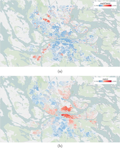
If the estimates are plotted according to their geographical position the spatial trend is clearly revealed, Figure 4. The spatial field, $\exp \left(\mathit{u}\right)$, is smooth in general, but there are some seemingly sharp edges. These are explained by ‘natural’ obstacles such as water. Areas separated by such an obstacle are not considered to be neighbours in the graph specification discussed in Section 3.2.

Figure 4. Map of Stockholm with the centroids of the areas coloured according to the expected values of $\exp \left({\mathit{z}}_i\mathit{\beta }\right)$ and $\exp \left(u_i\right)$ in the BYM model for frequency. (a) Estimates of the GLM-part, ${\mathrm{e}}^{{\mathit{z}}_i\mathit{\beta }},$ in the BYM model for frequency and (b) Estimates of the spatial part, ${\mathrm{e}}^{u_i}$, in the BYM model for frequency.

4.2.2. Evaluation of the severity models

In contrast to the frequency model, the severity model improves only slightly when adding random effects (iid, spatial, or both). In terms of DIC the BYM model is still best, but the gain is much smaller than for the frequency model. Considering the MSE for out of sample predictions the GLM model now provides the best performance; making the model choice less obvious for the severity data. Since the GLM model provides near optimal results with a simpler structure it will be preferred. Confirming the model choice, the estimated expected values of $\exp \left(u_i\right)$ in the BYM model were all in the interval $[0.996,1.002]$, indicating that the spatial effect adds very little to the model. To evaluate any residual spatial effect the expected values of ${\mathrm{e}}^{{\eta }_i}$ are obtained and prediction errors for the validation set are computed. The prediction errors seem to lack any spatial structure, Figure 5(b), again demonstrating that the GLM model is sufficient for modelling the severity data.

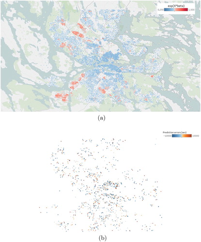
Figure 5. Predictions and prediction errors for the GLM model for severity. (a) Map of Stockholm with the centroids of the areas coloured according to the expected values of $\exp \left({\mathit{z}}_i\mathit{\beta }\right)$ in the GLM model for severity and (b) Normalized prediction errors in the GLM model for severity plotted according to their coordinates, no obvious remaining spatial structure can be seen. The predictions are made on the 10% validation set, excluding all areas with no claims. The map of Stockholm has been omitted to avoid obscuring the smaller prediction errors.

Plotting the estimates of $\mathsf{E}[\exp ({\mathit{z}}_i\mathit{\beta }\left)\right]$ from the GLM model for severity, Figure 5(a), reveals a geographical pattern similar to the covariate effect for claims frequency, Figure 4(a). This indicates that the two models are picking up the same underlying phenomena.

4.2.3. Performance of the geographical pricing model

Another type of model validation and performance testing is to fit the model on data from all areas, but leaving out a validation set of policies before aggregating the data to area level. A randomly selected validation set consisting of $15\mathrm{\%}$ of the available policies is set aside, and the BYM model for frequency and the GLM model for severity is fitted to the remaining data. In Table 4, the estimated total frequency and severity are displayed, together with the observed values for the left out policies. The resulting frequency estimate is very accurate, while the severity estimate is slightly high. These results seem consistent with the problems fitting anything more complex than a GLM model to the severity data. For further evaluation of the models see Tufvesson (2017).

Table 4. Estimated frequency and severity on the validation set of policies.

Measure	Estimate	Observation
Frequency	9.03%	8.99%
Severity	12,430	11,930

Note: The total duration of the policies in the validation set is 40,430 years.

5. Discussion and conclusions

Statistical models for the number of claims, Y, and claims cost, C, that allows for spatial dependence through spatial auto regression were introduced. The models were presented in a fully Bayesian framework and related to previous use in epidemiology and disease mapping (Waller & Carlin 2010, Blangiardo & Cameletti 2015). The entire analysis was performed using commonly available statistical software; the R-packages glmnet and INLA.

The models were demonstrated on vehicle hull damage policies using a high resolution spatial subdivision of Stockholm into 13,831 areas. Tractable inference for the high spatial resolution was obtained using INLA (Rue et al. 2009) as an alternative to MCMC. To handle the many potential covariates an elastic net (Zou & Hastie 2005) was used to extract a small set of candidate covariates and further covariate selection was performed using the marginal posteriors provided by INLA. Final model selection was performed using DIC and out of sample prediction errors.

The frequency model can be improved by adding both an unstructured, $\mathit{v}$, and a spatial effect, $\mathit{u}$, to the ordinary GLM model, yielding a BYM model (Besag et al. 1991). Since the hyper-parameters of the BYM model are estimated from data the magnitude of the spatial smoothing is completely data driven; eliminating any need for ad-hoc choices of smoothing parameters. The similarity between a BYM model with Poisson observations and a Besag model with negative binomial observations concur with results from Harrison (2014), who noted that adding observation level random effects to a Poisson model ‘appeared to robustly estimate the correct parameters at all but the highest levels of over-dispersion’. Further the frequency model was robust to the choice of priors, likely due to the very large dataset. However, the principled priors have shown impressive behaviour for smaller datasets (Simpson et al. 2017, Fuglstad et al. 2018) and are often easier to interpret (Sørbye et al. 2018).

For the severity model no significant improvement was identified when increasing model complexity. Thus the already popular GLM model was suggested for severity. The lack of spatial effect for the claims cost was not completely unexpected. Strong predictors, such as car brand and average income, are already accounted for in the weighted exposure, $E_i^{\ast }$. It might be that the spatial model for severity is more suitable for other policies, such as theft or third part liability. The predictive performance was encouraging for the frequency model, but unfortunately not as accurate for the severity model.

We acknowledge that the use of confidential covariates is problematic. However, the subset of covariates used in any given model will depend on data availability, legal restrictions, geographic regions, and modelled insurance policy. Thus, the main aim of this paper is to provide a statistical framework for how very large, spatially resolved datasets can be used to model claims frequency and severity.

5.1. Modelling alternatives

While the suggested modelling approach provides good results for the data studied, we would like to point out a few alternatives that might be relevant for other data. Firstly, the data used in this study allowed for the use of standard Poisson or negative binomial and gamma models for claims frequency and severity. Should the need arise the INLA package provides several alternative models (Bakka et al. 2018) including zero-inflated models for the counts; and log-normal, skew-normal, generalised extreme value (GEV) distributions or quantile regression (Opitz et al. 2018) for severity.

INLA provides some limited ability to model severity as spatial extremes by using a latent Gaussian field for one of the GEV parameters; more general versions of this modelling idea (i.e. spatial dependence in several parameters) can be fitted using MCMC (e.g. Cooley et al. 2007). A review of spatial extreme modelling (Davison et al. 2012) notes that latent variable models, as those described above, provide good fits for marginal distributions but copula models or max-stable processes (Koch 2017) are better suited to model joint distributions. A good starting point for spatial extremes might be the models provided in the SpatialExtremes R-package.

The two-step procedure used for variable selection ignores the spatial correlation when making the initial variable selection. It should, however, be noted that this initial selection only serves as a first filtering of suitable covariates and using a smaller λ in the elastic net allows for additional covariates to be considered in the spatial modelling step. An alternative, fully Bayesian approach would be to fit the model using a Metropolis Adjusted Langevin MCMC (Roberts & Stramer 2002) with horseshoe priors (Carvalho et al. 2009, Makalic & Schmidt 2016) for the variable selection (See e.g. Pirzamanbein et al. 2018, for an example on compositional data.). However, we fell that the potential gain of this model is unlikely to outweigh the added computational time and implementation complexity compared to our suggested approach using widely available software.

5.2. Extending the model to a larger area

Clearly, the division used here is on a very fine scale, with Stockholm divided into 13,831 areas. This is, to the extent of our knowledge, a spatial model for insurance risk on a much more detailed level than previously published. The fine spatial scale makes the MCMC inference proposed in Gschlößl & Czado (2007) very costly and probably infeasible. For both MCMC and INLA the computational costs associated with each likelihood evaluation grows as $\mathcal{O}\left(n^{3/2}\right)$ with the size, n, of the spatial subdivision (Rue & Held 2005, Ch. 2.3). The numerical optimisation in INLA is likely to benefit from larger datasets. However, the mixing of random walk MCMC algorithms (and thus the effective number of samples) scales as $\mathcal{O}\left(n^{-1/2}\right)$ (Roberts et al. 1997, Rosenthal 2011), implying that not only will the computational cost of each MCMC step increase but longer chains will be needed to obtain the same numerical accuracy.

Using INLA for approximate Bayesian inference makes the problem computationally tractable and should allow for models with ${10}^5$–${10}^6$ areas being solved on modern desktop computers (Rue et al. 2009). Since the granularity of the division decreases outside of Stockholm an ability to handle ${10}^5$–${10}^6$ areas should allow for a substantial geographical extension. Alternatively the computational burden could be reduced by fitting the model on each metropolitan region separately.

5.3. Other types of insurance

The case study here considered car insurance data. However, the outlined approach is applicable to other products in non-life insurance. The introduction of a pure spatial dependence might be an alternative solution in situations where it is hard to find suitable explanatory variables.

To wrap things up, accounting for spatial dependence when modelling insurance risk yields both better model fit and geographically resolved risk estimates, allowing for much better price differentiation between regions.

Disclosure statement

No potential conflict of interest was reported by the authors.

ORCID

Johan Lindström  http://orcid.org/0000-0001-9392-6053

Erik Lindström  http://orcid.org/0000-0002-6468-2624

Notes

1 Allowed rating factors depend on regulatory rules, since December 2012 gender is no longer permitted as a rating factor in the EU (IP/11/1581).

2 Personal communication with staff at If P&C Insurance

3 As a comparison there are 1009 zip codes areas in Stockholm,www.postnummerservice.se

References

- Assuncao R., Costa M. A., Prates M. O. & Silva e Silva L.s.G. (2014). Spatial analysis. In Charpentier, A., editor, Computational Actuarial Science with R. Boca Raton, FL: Chapman & Hall. P. 207–256.
- Bakka H., Rue H., Fuglstad G.-A., Riebler A., Bolin D., Illian J., Krainski E., Simpson D. & Lindgren F. (2018). Spatial modeling with R-INLA: a review. Wiley Interdisciplinary Reviews: Computational Statistics 10(6), e1443. doi: 10.1002/wics.1443
- Besag J. & Kooperberg C. (1995). On conditional and intrinsic autoregression. Biometrika82(4), 733–746.
- Besag J., York J. & Mollié A. (1991). Bayesian image restoration, with two applications in spatial statistics (with discussion). Annals of the Institute of Statistical Mathematics43, 1–59. doi: 10.1007/BF00116466
- Blangiardo M. & Cameletti M.2015). Spatial and spatio-temporal Bayesian models with R-INLA. Chichester: Wiley.
- Boskov M. & Verall R. J. (1994). Premium rating by geographic area using spatial models. Journal of the International Actuarial Association 24(1), 131–143.
- Carvalho C. M., Polson N. G. & Scott J. G. (2009). Handling sparsity via the Horseshoe. In van Dyk, D. and Welling, M., editors, Proceedings of the Twelfth International Conference on Artificial Intelligence and Statistics, volume 5 of Proceedings of Machine Learning Research, pages 73–80. PMLR.
- Cooley D., Nychka D. & Naveau P. (2007). Bayesian spatial modeling of extreme precipitation return levels. Journal of the American Statistical Association 102(479), 824–840. doi: 10.1198/016214506000000780
- Davison A. C., Padoan S. A. & Ribatet M. (2012). Statistical modeling of spatial extremes. Statistical Science 27(2), 161–186. doi: 10.1214/11-STS376
- Friedman J., Hastie T. & Tibshirani R. (2010). Regularization paths for generalised linear models via coordinate descent. Journal of Statistical Software 33(1), 1–22. doi: 10.18637/jss.v033.i01
- Fuglstad G.-A., Simpson D., Lindgren F. & Rue H. (2018). Constructing priors that penalize the complexity of Gaussian random fields. Journal of the American Statistical Association 0(0), 1–8. doi: 10.1080/01621459.2017.1415907
- Gschlößl S. & Czado C. (2007). Spatial modelling of claim frequency and claim size in non-life insurance. Scandinavian Actuarial Journal 2007(3), 202–225. doi: 10.1080/03461230701414764
- Harrison X. A. (2014). Using observation-level random effects to model overdispersion in count data in ecology and evolution. PeerJ 2(e616). Online.
- Hastie T., Tibshirani R. & Friedman J. (2001). The elements of statistical learning. New York: Springer. Springer Series in Statistics.
- Isham V. (2010). Spatial point process models. In Gelfand, A.E., Diggle, P., Guttorp, P., and Fuentes, M., editors. Handbook of Spatial Statistics. Boca Raton, FL: Chapman & Hall/CRC. P. 283–298.
- Knorr-Held L. & Rue H. (2002). On block updating in Markov random field models for disease mapping. Scandinavian Journal of Statistics 29(4), 597–614. doi: 10.1111/1467-9469.00308
- Koch E. (2017). Spatial risk measures and applications to max-stable processes. Extremes 20(3), 635–670. doi: 10.1007/s10687-016-0274-0
- Lindgren F. & Rue H. (2015). Bayesian spatial modelling with R-INLA. Journal of Statistical Software 63(19), 1–25. doi: 10.18637/jss.v063.i19
- Makalic E. & Schmidt D. F. (2016). A simple sampler for the horseshoe estimator. IEEE Signal Processing Letters 23(1), 179–182. doi: 10.1109/LSP.2015.2503725
- Mercer L. D., Szpiro A. A., Sheppard L., Lindström J., Adar S. D., Allen R. W., Avol E. L., A. P. Oron, Larson T., Liu L. J. & Kaufman J. D. (2011). Comparing universal kriging and land-use regression for predicting concentrations of gaseous oxides of nitrogen (NOx) for the multi-ethnic study of atherosclerosis and air pollution (MESA air). Atmospheric Environment 45(26), 4412–4420. doi: 10.1016/j.atmosenv.2011.05.043
- Ohlsson E. & Johansson B.2010). Non-life insurance pricing with generalized linear models. Berlin: Springer-Verlag.
- Okabe A., Boots B., Sugihara K. & Chiu S. N.2000). Spatial tessellations: concepts and applications of Voronoi diagrams. Chichester: Wiley.
- Opitz T., Huser R., Bakka H. & Rue H. (2018). INLA goes extreme: Bayesian tail regression for the estimation of high spatio-temporal quantiles. Extremes 21(3), 441–462. doi: 10.1007/s10687-018-0324-x
- Papoila A. L., Riebler A., Amaral-Turkman A., São João R., Ribeiro C., Geraldes C. & Miranda A. (2014). Stomach cancer incidence in Southern Portugal 1998–2006: a spatio-temporal analysis. Biometrical Journal 56(3), 403–415. doi: 10.1002/bimj.201200264
- Parodi P. (2012). Computational intelligence with applications to general insurance: a review: I – the role of statistical learning. Annals of Actuarial Science 6(2), 307–343. doi: 10.1017/S1748499512000036
- Pirzamanbein B., Lindström J., Poska A. & Gaillard M.-J. (2018). Modelling spatial compositional data: reconstructions of past land cover and uncertainties. Spatial Statistics 24, 14–31. doi: 10.1016/j.spasta.2018.03.005
- R Development Core Team (2013). R: a language and environment for statistical computing. Vienna, Austria: R Foundation for Statistical Computing.
- Roberts G., Gelman A. & Gilks W. (1997). Weak convergence and optimal scaling of random walk metropolis algorithms. Annals of Probability 7, 110–120. doi: 10.1214/aoap/1034625254
- Roberts G. O. & Stramer O. (2002). Langevin diffusions and metropolis-hastings algorithms. Methodology and Computing in Applied Probability 4(4), 337–357. doi: 10.1023/A:1023562417138
- Rosenthal J. S. (2011). Optimal proposal distributions and adaptive MCMC. In Brooks, S., Gelman, A., Jones, G.L., and Meng, X.-L., editors. Handbook of Markov Chain Monte Carlo. Boca Raton, FL: Chapman & Hall/CRC. P. 93–111.
- Rue H. & Held L. (2005). Gaussian Markov random fields; theory and applications. Boca Raton, FL: Chapman & Hall/CRC. Volume 104 of Monographs on Statistics and Applied Probability.
- Rue H. & Martino S. (2007). Approximate Bayesian inference for hierarchical Gaussian Markov random field models. Journal of Statistical Planning and Inference 137(10), 3177–3192. doi: 10.1016/j.jspi.2006.07.016
- Rue H., Martino S. & Chopin N. (2009). Approximate Bayesian inference for hierarchical Gaussian Markov random field models. Journal of the Royal Statistical Society: Series B (Statistical Methodology) 71(4), 319–392. doi: 10.1111/j.1467-9868.2008.00700.x
- Simpson D., Rue H., Riebler A., Martins T. G. & Sørbye S. H. (2017). Penalising model component complexity: a principled, practical approach to constructing priors. Statistical Science 32(1), 1–28. doi: 10.1214/16-STS576
- Sørbye S. H., Illian J. B., Simpson D. P., Burslem D. & Rue H. (2018). Careful prior specification avoids incautious inference for log-Gaussian Cox point processes. Journal of the Royal Statistical Society Series C 0(0), N/A.
- Tufvesson O. (2017). Spatial statistical modeling of insurance risk: an epidemiologist approach to improved car insurance. Master of science, Lund University, Lund, Sweden. LUTFMS–3313–2017.
- Waller L. & Carlin B. (2010). Disease mapping. In Gelfand, A.E., Diggle, P., Guttorp, P., and Fuentes, M., editors. Handbook of Spatial Statistics. Boca Raton, FL: Chapman & Hall/CRC. P. 217–243.
- Zou H. & Hastie T. (2005). Regularization and variable selection via the elastic net. Journal of the Royal Statistical Society: Series B (Statistical Methodology) 67(2), 301–320. doi: 10.1111/j.1467-9868.2005.00503.x