Stochastic modeling of assets and liabilities with mortality risk

ABSTRACT

This paper describes a general approach for the stochastic modeling of assets returns and liability cash-flows of a typical pensions insurer. On the asset side, we model the investment returns on equities and various classes of fixed-income instruments including short- and long-maturity fixed-rate bonds as well as index-linked and corporate bonds. On the liability side, the risks are driven by future mortality developments as well as price and wage inflation. All the risk factors are modeled as a multivariate stochastic process that captures the dynamics and the dependencies across different risk factors. The model is easy to interpret and to calibrate to both historical data and to forecasts or expert views concerning the future. This feature is particularly useful in unprecedented circumstances like pandemics when historical data alone does not give a reasonable description of the future. The simple structure of the model allows for efficient computations. The construction of a million scenarios takes only a few minutes on a personal computer. The approach is illustrated with an asset-liability analysis of a defined benefit pension fund, pre- and post-COVID-19.

Keywords:

• Investment
• longevity
• stochastic modeling

Subject classifications:

• Investment
• Insurance
• Stochastic modeling

1. Introduction

Stochastic simulation models have important applications in life and pension insurance. They are used in risk management, asset allocation, pricing and hedging of longevity-related products and in the valuation of pension liabilities. In the context of pensions, probably the best-known stochastic models are the CAP:LINK model built by Tillinghast Towers Perrin (now Towers Watson) (Mulvey 1996, Mulvey & Thorlacius 1998) and the Wilkie model (Wilkie 1984) for actuarial use in the UK. While the above are concerned with economic and financial risk factors, most life and pension insurers have major exposures also to mortality/longevity risk. This has sparked an active development of stochastic mortality models in the recent years but most models remain disconnected from the financial and economic risk factors; see e.g. Lee & Carter (1992), Hunt & Blake (2014) and Cairns et al. (2011) and their references.

This paper presents a general framework for the construction of stochastic simulation models for the assets and longevity-linked liabilities of a typical pension or life insurer. The framework accommodates longevity risk as well as the main asset classes used by pension funds: equities, short-term and long-term fixed-rate bonds, index-linked bonds and corporate bonds. Our models incorporate the often neglected dependencies between longevity and the economy; see Aro & Pennanen (2014) and Glover (2018). Such connections are important e.g. in valuation and hedging of long-dated longevity-linked products and liabilities. In long-dated liabilities, even weak statistical connections may allow for partial hedges that have strong effects on valuations and risk management. Our calibration approach allows also for the incorporation of forecasts or user views consistently with the statistical parameter estimates. This feature is crucial in many situations where the historical data does not give the best description of the future.

The present paper builds on several of our earlier papers on asset and liability modeling. As in Aro & Pennanen (2014) and Glover (2018), our stochastic model incorporates statistical connections between longevity and the economy. This paper employs the connections to develop a full-blown asset and liability simulation model where the connections affect returns in several asset classes. For bond portfolio returns, we use the reduced-form model from Koivu & Pennanen (2014) which gives accurate descriptions of returns even on large bond portfolios by using only one or two risk factors. This allows for convenient models for returns on money market investments, fixed-rate government bonds, corporate bonds as well as inflation-linked bonds. Moreover, we incorporate idiosyncratic default risk on corporate bonds that was ignored in the earlier studies. For longevity, we use the general approach of Aro & Pennanen (2011), where longevity/mortality-risks are described by interpretable population wide systemic risk factors together with idiosyncratic binomial risk factors describing yearly deaths. While the idiosyncratic risk can be diversified away by increasing the size of a fund, the systemic risk represents undiversifiable longevity risk. The explicit inclusion of the idiosyncratic risk makes the model ideal for studying the benefits of, e.g. mergers or consolidations of multiple pension funds. The systemic risk factors allow for natural interpretations which facilitates the calibration and analysis of the model. This is a significant advantage over, e.g. the famous Lee & Carter (1992) model and its refinements (see Cairns et al. 2011 for a review) where the risk factors are computed through a singular value decomposition which are not only difficult to interpret but also change every time new observations are added to the data.

After suitable nonlinear transformations, all the relevant risk factors are modeled by vector autoregressive (VAR) models much as in Koivu et al. (2005b), Koivu et al. (2005a), Aro & Pennanen (2014) and Wilkie & Sahin (2019). VAR models were recommended also in Wilkie & Sahin (2019) as an alternative to the cascading structures used in Wilkie (1984), Wilkie (1995), Mulvey (1996) and Mulvey & Thorlacius (1998). The VAR structure allows for more general dependencies across different risk factors. Moreover, VAR models lend themselves to efficient vectorized computations which allow the simulation of millions of scenarios within minutes on a personal computer; see Section 6.1.

A major advantage of our calibration approach is that it allows for the incorporation of short-term forecasts and/or long-term views concerning the median values of the risk factors in the model; see Section 4.2. Such subjective modifications were proposed also in Wilkie & Sahin (2016) and Wilkie (1984). We describe an easy procedure for the specification of the views and provide testable conditions that guarantee that the simulations indeed have the specified median values; see Proposition 4.1 in Section 4.2. One could also consider specifying user views concerning dependencies between various risk factors but we leave this for future research.

As an illustration of the general approach, we build a stochastic simulation model for UK pension funds. The modeled asset classes cover the majority of pension investments in the UK, namely, equities, short- and long-term fixed rate bonds, inflation-linked bonds and corporate bonds which, according to the ‘Purple Book’ Pension Protection Fund (2019), constitute approximately 90% of the UK pension assets. On the liability side, the model includes longevity risk as well as risks coming from the indexation of future pension benefits. The UK model is illustrated with a series of simulation experiments where we analyze the dynamics of population sizes, asset returns and macroeconomic risk factors that are statistically connected to both assets and liabilities. The simulation model was developed and implemented in Python 3.7 and run on an AMD Ryzen Threadripper 1950x desktop with 128 GB of RAM. Computation of one million random scenarios took 89 s.

The simulations show that idiosyncratic mortality risk is diversified away as cohort sizes are increased but it remains significant even in fairly large populations. We analyze the risks involved with defined benefit liabilities and consider the special case of the USS scheme in the UK. The risk contributions from longevity and indexation of the benefits vary with age and cohort sizes but over longer periods, both risks are significant. We also find a significant connection between economics and old age mortality, confirming the findings of Aro & Pennanen (2014) and Glover (2018) and establishing a link between longevity-linked liabilities and investment returns. We end the analysis with an asset-liability management (ALM) study where we simulate DB-pension schemes forward in time until run-off. We compare the performance of the average allocations of PPF-eligible schemes in 2008 and 2019. While the significant reduction in stock investments in 2019 results in lower overall uncertainty in future net wealth, the reduction is mainly on the upside while the downside risk slightly increases.

As an illustration of incorporating user views into the model, we compare the ALM-analyses under pre- and post-COVID-19 pandemic views. We combine the Office for Budget Responsibility's ‘Long-term economic determinants’ (Office for Budget Responsibility 2020b) and ‘Coronavirus reference scenario’ (Office for Budget Responsibility 2020a) with the parallel shift in mortality rates proposed, e.g. in Milevsky (2020). While the economic shock significantly lowers the asset values in the short term, it turns out that the simultaneous increases in mortality rates lower the pensions expenditure so that, at the end of the runoff period, the distribution of the net wealth of the fund is markedly better than with the pre-COVID-19 views.

The rest of the paper is organized as follows. Section 2 introduces some of the main risk factors that will be included in our model. Section 3 reviews inhomogeneous VAR-models and Section 4 presents our calibration approach. Sections 5 illustrates the modeling approach using UK data and Section 6 contains the simulation study.

2. Risk factors

The first step in the creation of any stochastic model is the identification of the most relevant risk factors that affect the quantities of interest. In the context of pension fund management, the interesting quantities are the investment returns in different asset classes and the pension expenditure. On the liability side, the most important sources of uncertainty are longevity, and price and wage inflation that are often used in indexation of defined benefit liabilities. There are also other macroeconomic risk factors, such as the gross domestic product (GDP), that may affect investment returns or liabilities indirectly. Indeed, it was found in Aro & Pennanen (2014) that GDP has an effect on old age mortality over longer periods of time. In Glover (2018), a similar link was found between old age mortality and average weekly earnings. GDP affects pension liabilities also through inflation which is often used in indexation of the benefits. GDP has statistically significant connections not only with inflation but also with many other factors that affect investment returns.

In a typical pension fund, one can easily identify thousands of risk factors that affect the assets and liabilities. Fortunately, it is often possible to come up with significant reductions in the number of risk factors while still capturing the main distributional properties of asset returns and liability payments. This section reviews some of the most relevant risk factors of a typical pension fund as well as some useful reductions for describing longevity and bond investments. A more detailed case study can be found in Section 5.

2.1. Longevity

Longevity risk is perhaps the most important source of risk faced by a defined benefit pension fund. There has been an increasing interest in stochastic modeling of longevity risk; see e.g. Cairns et al. (2011) and Hunt & Blake (2014). Common to all these models is the aim to describe the longevity risk across all relevant cohorts by a small number of risk factors whose future development is then modeled stochastically. We describe here the flexible approach from Aro & Pennanen (2011), which is easy to implement and allows for interpretable risk factors, more so than the famous Lee-Carter model Lee & Carter (1992).

We will denote the size of cohort aged a in year t by $E_{a,t}$. It is natural to assume that the future population sizes follow Binomial distributions with (1) $E_{a+1,t+1}\sim \mathrm{B}\mathrm{i}\mathrm{n}(E_{a,t};p_{a,t}),$(1) where $p_{a,t}$ is the survival probability of an individual aged a at the beginning of year t. For each year t, we assume that (2) $\mathrm{l}\mathrm{o}\mathrm{g}\mathrm{i}\mathrm{t}{p}_{a,t}:=\ln \left(\frac{p_{a,t}}{1-p_{a,t}}\right)=\sum _{i=1}^n{v}_t^i{\phi }^i\left(a\right),$(2) where ${\phi }^i$ are a given collection of basis functions and $v_t^i$ are the corresponding risk factors that may vary over time and across different scenarios. Thus, instead of considering the survival probability in each age cohort as a separate risk factor, we describe the probabilities of all ages by the n risk factors $v^i$ with n much less than the number of ages considered. This reduction facilitates both the stochastic modeling of the future survival probabilities as well as their numerical simulation; see Section 6.1. The interpretation of the risk factors $v^i$ depends on the choice of the corresponding basis function ${\phi }^i$. With the choices made in Aro & Pennanen (2014), each factor corresponds to the logistic survival probability of an age group; see also Section 5.1.1.

Historical values of the risk factors $v_t^i$ are obtained by maximizing, year by year, the likelihood function ${\mathcal{L}}_t\left(v_t\right):=\sum _{a\in A}\left[0()E_{a,t}-D_{a,t}\sum _{i=1}^n{v}_t^i{\phi }^i\left(a\right)-E_{a,t}\ln \left(1+\mathrm{e}\mathrm{x}\mathrm{p}0()\sum _{i=1}^n{v}_t^i{\phi }^i\left(a\right)\right)\right],$where $D_{a,t}$ is the number of deaths of individuals aged $[a,a+1)$ in year t. The function ${\mathcal{L}}_t$ is concave, which greatly facilitates its maximization; see Aro & Pennanen (2011, Proposition 3).

We model the future development of the risk factors v stochastically in a joint model with other relevant risk factors. While the uncertainty concerning the development of v may be interpreted as systemic risk, the uncertainty concerning the binomial cohort sizes is an idiosyncratic risk that may be reduced with diversification. Such diversification effects are the key factors when considering mergers and consolidations of pension funds and schemes.

2.2. Investments

On the investment side, our aim is to describe the future returns in typical asset classes of pension funds. As we are concerned with long-term strategic investments, we will group investments in broader classes as is often done is strategic asset-liability management. Assets can be grouped in many different ways but for purposes of asset allocation, the most useful is done according to the statistical properties of the returns.

In the present work, we concentrate on the asset classes most relevant to UK pension funds. According to Table 1, extracted from the ‘Purple Book’ (Pension Protection Fund 2019), nearly 90% of the UK pension funds are allocated in equities, bonds, property and cash and deposits.

Table 1. Asset allocation in total assets for DB pension schemes in the Purple Book data set (weighted averages).

Year	Equities	Bonds	Property	Cash and deposits	Insurance policies	Hedge funds	Annuities	Misc.
2008	53.6%	32.9%	5.6%	3.0%	1.1%	n/a	n/a	3.8%
2009	46.4%	37.1%	5.2%	3.9%	1.4%	1.5%	n/a	4.5%
2010	42.0%	40.4%	4.6%	3.9%	1.4%	2.2%	n/a	5.4%
2011	41.1%	40.1%	4.4%	4.1%	1.6%	2.4%	n/a	6.3%
2012	38.5%	43.2%	4.9%	5.1%	0.2%	4.5%	n/a	3.6%
2013	35.1%	44.8%	4.7%	6.7%	0.1%	5.2%	n/a	3.5%
2014	35.0%	44.1%	4.6%	6.1%	0.1%	5.8%	n/a	4.3%
2015	33.0%	47.7%	4.9%	3.5%	0.1%	6.1%	n/a	4.7%
2016	30.3%	51.3%	4.8%	3.0%	0.1%	6.6%	2.1%	1.7%
2017	29.0%	55.7%	5.3%	−0.9%	0.1%	6.7%	3.3%	0.8%
2018	27.0%	59.0%	4.8%	−2.5%	0.1%	7.0%	3.4%	1.2%
2019	24.0%	62.8%	5.0%	−4.4%	0.3%	7.4%	4.0%	1.0%

Liquid equity investments are described, as usual, by a total return index P that tracks the changes in value due to price movements as well as dividend payments. Yearly equity returns are then given simply by $R_t=P_t/P_{t-1}$.

Bond investments can be grouped according, e.g. to maturities, credit ratings and the possible underlying indices. Table 2 gives a breakdown of the UK pension fund bond investments; see Pension Protection Fund (2019).

Table 2. Proportions of bond investment by DB pension schemes in the Purple Book data set (weighted averages).

Year	Government fixed interest	Corporate fixed interest	Index-linked
2008	33.2%	32.6%	33.9%
2009	29.0%	38.3%	32.6%
2010	24.6%	42.2%	33.1%
2011	19.6%	44.3%	36.1%
2012	17.7%	44.8%	37.5%
2013	18.5%	40.6%	40.9%
2014	18.6%	40.3%	41.1%
2015	20.3%	37.7%	42.0%
2016	21.9%	33.7%	44.4%
2017	24.1%	31.4%	44.5%
2018	24.1%	28.8%	47.1%
2019	25.4%	28.4%	46.2%

For bond investments, we will use the approximation from Koivu & Pennanen (2014) that describes investment returns on bond portfolios using only two risk factors, the yield to maturity and the underlying index. Consider a bond or a portfolio of bonds with outstanding payments at times $t_1<t_2<\cdots <t_N$. The portfolio's yield to maturity (YTM) $Y_t$ at time $t<t_1$ is defined as the solution of the equation (3) $P_t=\sum _{n=1}^N{e}^{-Y_t(t_n-t)}{I}_t{c}_n,$(3) where $P_t$ is the portfolio's market price, $c_n$ are the outstanding payments and $I_t$ is an index. Fixed rate bonds correspond to a constant I while in the case of inflation-linked bonds, I is the consumer/retail price index. The index can also be used to describe default risk in corporate bonds. In that case, I is the recovery index that describes the reduction of the outstanding payments due to defaults of bond issuers.

As shown in Koivu & Pennanen (2014), the first-order Taylor approximation of the logarithmic price with respect to time, the YTM and the index gives (4) $\mathrm{\Delta }\ln P\approx Y_t\mathrm{\Delta }t-D_t\mathrm{\Delta }Y+\mathrm{\Delta }\ln I,$(4) where $\mathrm{\Delta }Y:=Y_s-Y_t$, $\mathrm{\Delta }\ln I=\ln I_s-\ln I_t$ and $D_t:=\frac{1}{B_t}\frac{\mathrm{\partial }{B}_t}{\mathrm{\partial }Y}=\frac{1}{B_t}\sum _{n=1}^N(t_n-t)e^{-Y_t(t_n-t)}{c}_n{I}_t$is the duration of the portfolio. Thus, the portfolio return is approximated by $\frac{P_s}{P_t}\approx \exp \left(Y_t\mathrm{\Delta }t-D_t\mathrm{\Delta }Y+\mathrm{\Delta }\ln I\right).$This simple formula expresses the return on a bond portfolio in terms of only two risk factors, the YTM and the underlying index. A possibly very complicated structure of the outstanding payments is captured by a single characteristic, the duration. Statistical analysis of Koivu & Pennanen (2014) on bond data from six different countries shows that formula (4(4) $\mathrm{\Delta }\ln P\approx Y_t\mathrm{\Delta }t-D_t\mathrm{\Delta }Y+\mathrm{\Delta }\ln I,$(4) ) explains consistently more than 99% of the variance of the log-returns on bond portfolios.

Similarly, the second-order Taylor's approximation gives (5) $\mathrm{\Delta }\ln P\approx Y_s\mathrm{\Delta }t-D_t\mathrm{\Delta }Y+\frac{1}{2}(C_t-D_t^2)(\mathrm{\Delta }Y{)}^2+\mathrm{\Delta }\ln I,$(5) where $C_t:=\frac{1}{B_t}\frac{{\mathrm{\partial }}^2{B}_t}{\mathrm{\partial }{Y}^2}=\frac{1}{B_t}\sum _{n=1}^N(t_n-t{)}^2{e}^{-Y_t(t_n-t)}{I}_t{c}_n,$is the convexity of the bond portfolio. The analysis of Koivu & Pennanen (2014) suggests, however, that the second-order terms do not add much precision as the first-order approximation is already nearly perfect. This applies also to the bond portfolios studied in this paper; see Table 6.

3. The stochastic model

Our aim is to construct a stochastic model that provides a reasonable description of the future development of the relevant risk factors and thus, of the asset returns and liability cash-flows. What is reasonable depends, to a large extent, on subjective views and knowledge concerning the involved risk factors. We will develop a simple model that allows for an easy calibration to both the user's views and to historical data.

In order to capture certain natural features of the risk factors, we start by applying invertible transformations to the original ones. For example, it is common to model the logarithms of various price processes when they are known to stay positive in all scenarios. A general yet simple approach is described in the classic paper of Box & Cox (1964). With appropriate transformations, one can often get away with Gaussian processes in modeling the transformed risk factors; see Section 5 for a case study with UK data.

We will model the future development of the transformed risk factors $x_t$, by a multivariate stochastic difference equation of the form (6) $\mathrm{\Delta }{x}_t=A{x}_{t-1}+a_t+{\epsilon }_t,$(6) where $\mathrm{\Delta }{x}_t:=x_t-x_{t-1}$, A is a square matrix, $a=(a_t{)}_{t\ge 0}$ is a given sequence and ${\epsilon }_t$ are zero-mean random (innovation) vectors all of appropriate dimensions. This can be written as an inhomogeneous vector autoregressive time series model $x_t=(A+I)x_{t-1}+a_t+{\epsilon }_t.$Vector autoregressive models have been extensively studied in the literature; see e.g. Sims (1980) and Hamilton (1994). Applications to macroeconomic modeling can be found in Canova (1999), Bjornland (2000), Koivu et al. (2005b), Koivu et al. (2005a), Aro & Pennanen (2014) and Wilkie & Sahin (2019). One may view (6(6) $\mathrm{\Delta }{x}_t=A{x}_{t-1}+a_t+{\epsilon }_t,$(6) ) also as a time-discretization of the linear inhomogeneous stochastic differential equation $\mathrm{d}{x}_t=(\tilde{A}{x}_t+{\tilde{a}}_t)\mathrm{d}t+\mathrm{d}{W}_t,$where W is a martingale whose increments correspond to ϵ in (6(6) $\mathrm{\Delta }{x}_t=A{x}_{t-1}+a_t+{\epsilon }_t,$(6) ). Continuous time stochastic differential equations have been used, e.g. in the stochastic asset model CAP:Link built by Tillinghast Towers Perrin (now Towers Watson); see Mulvey (1996) and Mulvey & Thorlacius (1998).

Already in the scalar case, (6(6) $\mathrm{\Delta }{x}_t=A{x}_{t-1}+a_t+{\epsilon }_t,$(6) ) subsumes many well known stochastic process models as special cases. If A = 0 we obtain a discrete-time version of the classical Brownian motion with drift $a=(a_t{)}_{t\ge 0}$. If x is the logarithm of the stock price, we then recover a discrete-time version of the classical geometric Brownian motion.

Another instance of (6(6) $\mathrm{\Delta }{x}_t=A{x}_{t-1}+a_t+{\epsilon }_t,$(6) ) is the mean reversion model $\mathrm{\Delta }{x}_t=-\alpha (x_{t-1}-c)+{\epsilon }_t,$where the parameters c and α determine the mean and the speed of mean reversion, respectively. If x is the logarithm of an interest rate, we recover the Black–Karasinski interest rate model Black & Karasinski (1991).

The multivariate VAR-format gives a natural way of describing interactions between different risk factors without having to specify directional causalities as in the classic Wilkie model (Wilkie 1984). Note that dependencies can come from the autoregression matrix A or through the dependencies between the components of the innovation vectors ${\epsilon }_t$. Imaginary eigenvalues of the matrix A result in oscillatory behavior of x which is often observed in the long-term analysis of various macroeconomic variables (Hamilton 1994). A single instance of (6(6) $\mathrm{\Delta }{x}_t=A{x}_{t-1}+a_t+{\epsilon }_t,$(6) ) can describe stationary, mean-reverting and even cointegrated risk factors. Indeed, the vector error correction model (see e.g. Engle & Granger 1987) $\mathrm{\Delta }{x}_t=\alpha (\text{β}{x}_{t-1}-c)+d+{\epsilon }_t,$is also an instance of (6(6) $\mathrm{\Delta }{x}_t=A{x}_{t-1}+a_t+{\epsilon }_t,$(6) ). This format was used in the context of pensions in Koivu et al. (2005a).

Through the term $a=(a_t{)}_{t\ge 0}$, one can incorporate forecasts and expert views concerning the future; see Section 4.2. This is a particularly important feature in long-term applications where the historical data may be a poor description of the future. For example, developments in monetary policy, medicine and lifestyle have changed the way we now view interest rates, inflation and mortality developments. When specifying views concerning specific risk factors, it is important that the risk factors have natural interpretations. Such interpretations may be lost in approaches based on modeling principal components or singular values as in the Lee-Carter model of mortality (Lee & Carter 1992).

4. Model calibration

In order to get a reasonable description of the future, we will calibrate (6(6) $\mathrm{\Delta }{x}_t=A{x}_{t-1}+a_t+{\epsilon }_t,$(6) ) to both historical data as well as expert views/forecasts concerning the future. User views are particularly important when the historical values of the risk factors do not correspond to what one expects to see in the future. In particular, due to improvements in healthcare and monetary policy, most of us expect mortality and interest rates to be lower in the future than 50 years ago. The historical values may, nevertheless, still exhibit dependencies that one expects to prevail in the future as well. Accordingly, we calibrate the parameters of the model in two steps: we first estimate the parameter matrix A as well as the distribution of the innovations ${\epsilon }_t$ using historical data and, in the second step, we incorporate user's views by an appropriate specification of the sequence $(a_t{)}_{t\ge 1}$.

4.1. Calibration to historical data

The elements of the autoregression matrix A are estimated by linear regression after a careful selection of the explanatory variables. We aim for a parsimonious model where we retain only the regressors that are both statistically significant and have an economic justification. We also perform a simple robustness test to validate the regressions, by varying the estimation window. Similar tests have been suggested in Huber (1997) and Wilkie et al. (2011). All the elements of A should remain statistically significant and have signs consistent with economic theory.

The above restrictions are important in practice since relying on statistical significance alone often leads to spurious regressions and poor descriptions of the dynamics of the risk factors. As an additional consistency check, we compute the eigenvalues of A + I. If we know, for example, that all the risk factors x are all stationary, the eigenvalues of $(A+I)$ should all lie strictly inside the unit circle in the complex plane. Nonstationary risk factors $x^i$ whose increments $\mathrm{\Delta }{x}^i$ are stationary correspond to eigenvalues on the unit circle. Imaginary eigenvalues result in oscillations which may be associated with economic cycles.

Once the autoregression matrix A has been estimated, we use the regression residuals to estimate the distribution of the innovations ${\epsilon }_t$. In the simplest case, a multivariate Gaussian distribution is used. Alternatives include multivariate t-distribution and copula models. One could also use more complicated stochastic volatility models such as multivariate GARCH models as, e.g. in Hilli et al. (2011) and Van der Weide (2002).

4.2. Incorporating views and forecasts

Asset managers base their investment decisions on their best knowledge and views concerning the future investment returns. The returns are highly uncertain but with proper financial/statistical analysis, the best asset managers tend to guess the returns better than the average person. The importance of views and educated guesses is pronounced in pension funds that aim to cover the uncertain pension expenditure in the future. Such views also have a strong effect on the valuation of pension liabilities and the pricing of life insurance products.

In the inhomogeneous VAR model (6(6) $\mathrm{\Delta }{x}_t=A{x}_{t-1}+a_t+{\epsilon }_t,$(6) ), one can incorporate views on the future mean values $\overline{x}$ of x by an appropriate specification of the sequence $(a_t{)}_{t\ge 1}$. To this end, the following simple observation is useful.

Lemma 4.1

A stochastic process $x=(x_t{)}_{t\ge 0}$ given by (6(6) $\mathrm{\Delta }{x}_t=A{x}_{t-1}+a_t+{\epsilon }_t,$(6) ) has the decomposition $x=\overline{x}+e$, where the mean $\overline{x}=({\overline{x}}_t{)}_{t\ge 0}$ follows the deterministic difference equation (7) $\mathrm{\Delta }{\overline{x}}_t=A{\overline{x}}_{t-1}+a_t$(7) with ${\overline{x}}_0=x_0$ and e is a zero-mean process following homogeneous VAR (8) $\mathrm{\Delta }{e}_t=A{e}_{t-1}+{\epsilon }_t$(8) with $e_0=0$. In particular, if we have a forecast $({\overline{x}}_t{)}_{t\ge 0}$ and define (9) $a_t:=\mathrm{\Delta }{\overline{x}}_t-A{\overline{x}}_{t-1},$(9) then x has mean $({\overline{x}}_t{)}_{t\ge 0}$.

Proof.

The mean of x follows (6(6) $\mathrm{\Delta }{x}_t=A{x}_{t-1}+a_t+{\epsilon }_t,$(6) ) with the innovations ϵ set to zero. This is (7(7) $\mathrm{\Delta }{\overline{x}}_t=A{\overline{x}}_{t-1}+a_t$(7) ), or equivalently, (9(9) $a_t:=\mathrm{\Delta }{\overline{x}}_t-A{\overline{x}}_{t-1},$(9) ). The claims now follow from the fact that the process e has zero mean and that $x=\overline{x}+e$, by linearity.

To incorporate the future views into the inhomogeneous VAR (6(6) $\mathrm{\Delta }{x}_t=A{x}_{t-1}+a_t+{\epsilon }_t,$(6) ) one can thus first specify the mean values $\overline{x}$ and then define a by (9(9) $a_t:=\mathrm{\Delta }{\overline{x}}_t-A{\overline{x}}_{t-1},$(9) ). However, one rarely has a forecast $\overline{x}=({\overline{x}}_t{)}_{t\ge 1}$ indefinitely far into the future. Instead, forecasts are usually available only for some of the risk factors and only for a few years into the future. In addition to short-term forecasts, one may have views on long-term mean values of, e.g. interest rates, inflation and various investment returns. We will construct a mean trajectory $\overline{x}$ which is consistent with such forecasts and views as well as with the estimated parameter matrix A.

Consider the vector error correction (VECM) model (10) $\mathrm{\Delta }{x}_t=\alpha (\text{β}{x}_{t-1}-c)+d+{\epsilon }_t,$(10) where $\text{β}\in R{R}^{m\times n}$, $\alpha \in R{R}^{n\times m}$, $c\in R{R}^m$ and $d\in R{R}^n$. Note that this is a special case of (6(6) $\mathrm{\Delta }{x}_t=A{x}_{t-1}+a_t+{\epsilon }_t,$(6) ) with $A=\alpha \text{β}$ and $a_t=d-\alpha c$ for all t. Conversely, an autonomous VAR-model (one with $a_t$ independent of t) can be written in the VECM-form with e.g. $\alpha =I$, $\text{β}=A$, c = 0 and d = a. The VECM-representation (10(10) $\mathrm{\Delta }{x}_t=\alpha (\text{β}{x}_{t-1}-c)+d+{\epsilon }_t,$(10) ) is not unique but, if there is one that satisfies the assumptions in Proposition 4.1, then $\mathrm{\Delta }x$ and $\text{β}x$ have long-term means equal to d and c, respectively. A necessary condition for this to hold is that $\text{β}d=0$ since otherwise one of the equilibrium conditions would necessarily be violated. Asymptotic properties of multivariate time series models have been analyzed e.g. in Lütkepohl (2005). For the first-order model (10(10) $\mathrm{\Delta }{x}_t=\alpha (\text{β}{x}_{t-1}-c)+d+{\epsilon }_t,$(10) ), we get the following particularly convenient result.

Proposition 4.1

If $\text{β}d=0$ and the eigenvalues of the matrix $I+\text{β}\alpha \in R{R}^{m\times m}$ are strictly within the unit circle, then any solution x of (10(10) $\mathrm{\Delta }{x}_t=\alpha (\text{β}{x}_{t-1}-c)+d+{\epsilon }_t,$(10) ) satisfies $E\left[\text{β}{x}_t\right]\to c\mathrm{a}\mathrm{n}\mathrm{d}E\left[\mathrm{\Delta }{x}_t\right]\to d.$

Proof.

Taking expectations on both sides of (10(10) $\mathrm{\Delta }{x}_t=\alpha (\text{β}{x}_{t-1}-c)+d+{\epsilon }_t,$(10) ) gives (11) $\mathrm{\Delta }{\overline{x}}_t=\alpha (\text{β}{\overline{x}}_{t-1}-c)+d,$(11) where ${\overline{x}}_t=E{x}_t$. Let ${\overline{z}}_t=\text{β}{\overline{x}}_t-c$. We have $\begin{array}{rl}\mathrm{\Delta }{\overline{z}}_t& =\text{β}\mathrm{\Delta }{\overline{x}}_t\\ & =\text{β}\left[\alpha \right(\text{β}{\overline{x}}_{t-1}-c)+d]\\ & =\text{β}\alpha {\overline{z}}_{t-1},\end{array}$where the last equality holds since $\text{β}d=0$, by assumption. It follows that $\begin{array}{rl}{\overline{z}}_t& =(I+\text{β}\alpha ){\overline{z}}_{t-1}\\ & =(I+\text{β}\alpha {)}^2{\overline{z}}_{t-2}\\ & ⋮\\ & =(I+\text{β}\alpha {)}^t{\overline{z}}_0.\end{array}$The eigenvalue condition implies $\underset{t\to \mathrm{\infty }}{lim}(I+\text{β}\alpha {)}^t=0$as can be seen by writing the matrix $(I+\text{β}\alpha )$ in its Jordan form; see e.g. Lütkepohl (2005, page 657). Thus, ${\overline{z}}_t\to 0$, or in other words, $E[\text{β}{x}_t-c]\to 0$, which proves the first claim. It is clear from (11(11) $\mathrm{\Delta }{\overline{x}}_t=\alpha (\text{β}{\overline{x}}_{t-1}-c)+d,$(11) ) that this, in turn, implies $\mathrm{\Delta }{\overline{x}}_t\to d$, or in other words, $E\left[\mathrm{\Delta }{x}_t\right]\to d$

Proposition 4.1 allows us to specify views on the long-term mean growth $\mathrm{\Delta }x$ and the long-term mean levels of the stationary series $\text{β}x$. The former can be used to express views, e.g. on the stock returns, mortality and other drifting risk factors, while the latter allows us the specify views, e.g. on the levels of interest rates, bond yield and inflations.

To combine the long-term views with possible short-term forecasts, we define the mean trajectory recursively by ${\overline{x}}_0:=x_0$ (the current values of the risk factors) and $\mathrm{\Delta }{\overline{x}}_t=\alpha (\text{β}{\overline{x}}_{t-1}-c)+dt=1,2,\dots$where, at each step, we overwrite the values of those components of ${\overline{x}}_t$ for which forecasts are available. The inhomogeneous VAR model (6(6) $\mathrm{\Delta }{x}_t=A{x}_{t-1}+a_t+{\epsilon }_t,$(6) ) is then specified by defining the sequence a according to Lemma 4.1.

Remark 4.1

Medians vs. means

When specifying views and forecasts, it is often more convenient to specify medians instead of means. When the innovations are Gaussian or more general symmetrically distributed random variables, there is no difference between the two but the components of x are often obtained through nonlinear monotone transformations of various economic risk factors. Medians pass directly through such transformations but means do not. More specifically, if $x^i=g^i\left(X^i\right)$ where $X^i$ is a random variable with median ${\overline{X}}^i$ and $g^i$ is a monotone function, then $x^i$ has median $g^i\left({\overline{X}}^i\right)$. Conversely, specifying the median of $x^i$ according to Proposition 4.1, we can specify the future medians of $X_t^i$. Indeed, if $g^i$ is strictly increasing, then for every $q\in RR$, $P\left(g^i\right(X^i)\le g^i(q\left)\right)=P(X^i\le q)$so all the quantiles of $g^i\left(X^i\right)$ are obtained by applying $g^i$ to the corresponding quantiles of $X^i$.

Proposition 4.1 and Remark 4.1 will be illustrated in Section 5.3.4 in the calibration of a model for UK pension insurers.

5. An implementation for the UK

Following the approach presented above, we now develop a stochastic model for UK pension insurers. We illustrate the techniques of Section 4.2 on the inclusion of user views by calibrating the model to the macroeconomic forecasts published by the Office for Budget Responsibility (Office for Budget Responsibility 2020b). The model also incorporates statistical dependencies between longevity and the economic risk factors. In particular, we find both long-term cointegration effects as well as short-term correlations between the longevity risk factors and the economic variables.

On the asset side, the model incorporates the most important asset classes used by pension funds in the UK, as described in the Purple Book: cash and deposits (short-term fixed income instruments), equities, government bonds, inflation-linked bonds and corporate bonds. Additional asset classes can be easily included, if necessary. On the liabilities side, the model incorporates mortality risk as described in Section 2.1. In addition, the model incorporates the average weekly earnings (AWE), GDP growth and inflation. Earlier works on stochastic simulation models for UK pensions include the Wilkie model (Wilkie 1984) and the PPI-model (Armstrong et al. 2013), but neither of them considered mortality risk.

5.1. Historical data

Finding appropriate historical data for the calibration of high-dimensional models with various economic as well as longevity risk factors can be challenging. First, one must deal with the different sampling frequencies found in time series data. Financial data, such as stock indices and bond yields, is often available on a daily basis, while macroeconomic indicators such as inflation and GDP are usually available only monthly or quarterly. On a national level, demographic data is only available on a yearly basis. In addition, the available time series usually span different periods of time. Here, we deal with the first problem by adopting the lowest sampling frequency found in the available data sets, and with the second problem by splicing closely related time series.

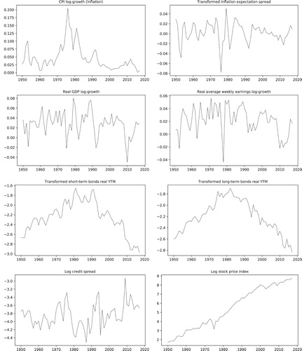
We will use the database ‘A Millennium of Macroeconomic Data’ (Thomas & Dimsdale 2017), an extensive collection of spliced time series data on the UK economy that has been organized in the Bank of England. This database was our main source of data, as it supplied the historical yields used to extend the bond indices collected from the ICE Index Platform (Intercontinental Exchange 2019), and the macroeconomic indicators used in the project: the gross domestic product (GDP), the consumer price index (CPI) and the average weekly earnings (AWE). For the estimation of survival probabilities, we have used demographics data for the UK from the Human Mortality Database University of California, Berkeley. In the following sections, we describe in more detail the historical data used in the estimation of parameters for the risk factors in our model (Figure 1).

Figure 1. Historical data used in the calibration of the time series model.

5.1.1. Survival probabilities

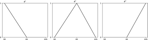
Once a set of basis functions is specified, survival probabilities can be easily estimated from demographics data by maximizing the likelihood function shown in Section 2.1. Following Aro & Pennanen (2011), we adopt three risk factors for each gender, and the piecewise linear basis functions ${\phi }^1\left(x\right)=\left\{\begin{array}{ll}\frac{65-x}{47}& x\le 65\\ 0& x\ge 65\end{array}\right.,{\phi }^2\left(x\right)=\left\{\begin{array}{ll}\frac{x-18}{47}& x\le 65\\ \frac{105-x}{40}& x\ge 65\end{array}\right.,{\phi }^3\left(x\right)=\left\{\begin{array}{ll}0& x\le 65\\ \frac{x-65}{40}& x\ge 65\end{array}\right.;$see Figure 2. Equation (2(2) $\mathrm{l}\mathrm{o}\mathrm{g}\mathrm{i}\mathrm{t}{p}_{a,t}:=\ln \left(\frac{p_{a,t}}{1-p_{a,t}}\right)=\sum _{i=1}^n{v}_t^i{\phi }^i\left(a\right),$(2) ) implies that $v_t^1=\mathrm{l}\mathrm{o}\mathrm{g}\mathrm{i}\mathrm{t}{p}_{18,t},v_t^2=\mathrm{l}\mathrm{o}\mathrm{g}\mathrm{i}\mathrm{t}{p}_{65,t},v_t^3=\mathrm{l}\mathrm{o}\mathrm{g}\mathrm{i}\mathrm{t}{p}_{105,t},$i.e, $v_t^1$, $v_t^2$ and $v_t^3$ are the logistic survival probabilities of the 18-, 65- and 105-year-old individuals. Such simple interpretations of the risk factors facilitates the development of stochastic models as it helps assessing the sensibility of parameter estimates and, in particular, the incorporation of views concerning the future development of the factors.

Figure 2. Set of basis functions used in the estimation of the historical mortality risk factors. With this particular choice, the risk factors $v^1$, $v^2$ and $v^3$ correspond to logistic survival probabilities of cohorts with age 18, 65 and 105.

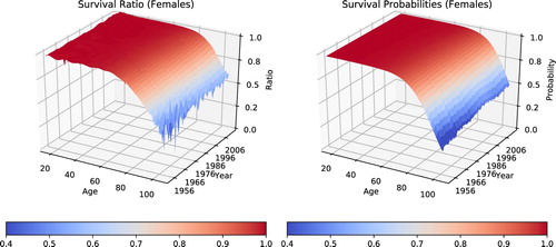
Using historical population sizes and numbers of deaths for the UK from the Human Mortality Database University of California, Berkeley, we estimated the yearly historical longevity risk factors in the period between the years 1922 and 2016. The yearly values are plotted in Figure 3. As one would expect, the logistic survival probabilities decrease with age, and, in general, females have a larger chance of survival than males of similar age. There is a strong positive trend in all ages but the younger cohorts seem to have already reached a saturation level. Similar phenomena can be observed in most developed countries (Aro & Pennanen 2014). One can also observe a decrease in the survival probabilities of young males during the Second World War. Figure 4 plots the historical survival ratios $E_{a+1,t+1}/E_{a,t}$ and the estimated survival probabilities for comparison. The overall shapes are similar but, as expected, the probability surfaces are smoother as they do not incorporate the idiosyncratic binomial risk.

Figure 3. Historical values for the mortality risk factors in the UK. The comparison of the risk factors in the plot shows that survival probabilities decrease with increasing age ($v^1>v^2>v^3$) and that, in general, females are more likely to survive than males of similar age ($v^f>v^m$). The plots also show an interesting feature that is captured by the model: a decrease in the survival probabilities of young males during World War II.

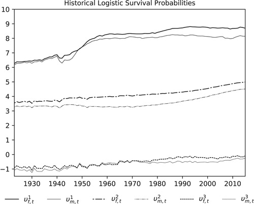
Figure 4. Comparison of historical survival ratios ($\frac{E_{a+1,t+1}}{E_{a,t}}$) with the corresponding estimated survival probabilities for females in the UK.

5.1.2. Short-term bonds

Returns for the portfolio of short-term bonds in our model are based on the YTMs of the ‘ICE BofA 1-4 Year UK Gilt Index’, found in the ICE Index Platform with the code GFL0. Given the short length of this time series, we extend it with the ‘Bank of England/Official Interest Rates in the UK’ yields for the period between 1948 and 1998, found in the Millennium database. The values recorded in the time series match quite well, as illustrated in Figure 5, where the daily values of the YTM for the ICE index is plotted against the the annual average values found in the Millennium database.

Figure 5. The pictures illustrate the matching of historical yields found in the Millennium database and in the ICE Index Platform. Yearly values from the latter were spliced with values from the first to provide the long time series necessary for the calibration of the time series model.

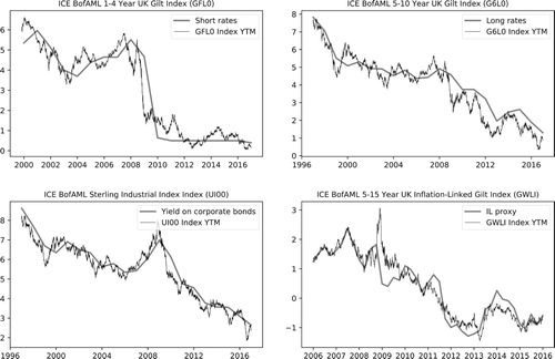
5.1.3. Long-term bonds

For the portfolio of long-term government bonds, we adopt the ‘ICE BofA 5-10 Year UK Gilt’ fixed income index, with code G6L0 in the ICE Index Platform. As for short-term bonds, we obtain the YTM of the portfolio by splicing two time series. In this case, the G6L0 index and the ‘Yield on 10 year/medium-term British Government Securities’ historical yields (1948–1991) from the Millennium database. In the top-right corner of Figure 5, one can notice how well both time series match.

5.1.4. Inflation-linked bonds

For the YTM of our portfolio of inflation-linked bonds (ILBs), we adopt the difference between the yields on long-term government bonds and long-term inflation expectations (LTIE), both found in the Millennium database. This proxy matches the YTM of the ‘ICE BofA 5-15 Year UK Inflation-Linked Gilt Index’ (GWLI) fixed income index, as illustrated in Figure 5.

5.1.5. Corporate bonds

The YTMs of the portfolio of corporate bonds are obtained by extending the ‘ICE BofA Sterling Industrial Index’ (UI00) index with the historical yields found in the Millennium database for the years between 1948 and 1996. These correspond to a spliced series of ‘Yield on debentures, loan stocks and other corporate bonds 1945–2005’ that have been collected from several sources and the ‘Sterling Corporate bond yields on industrials rated AAA-BBB’ fixed income index from BofA Merrill Lynch Global Research. As shown in Figure 5, the YTM time series match quite well.

5.1.6. Stock index

The stock index in our model corresponds to the ‘FTSE All-share’ total return index (1985–2019) spliced with the stock price index found in the Millennium database. The latter is composed of the ‘Actuaries’ Investment index of ordinary industrial shares', obtained from the Monthly Digest of Statistics, and the ‘FTSE All-share’ index, scaled to 100 in the 10th of April, 1962. To account for dividends, an additional 3.6% yearly return was included in the Millennium database's stock price index. This level corresponds to the mean difference between the log-returns of the ‘FTSE All-share’ price and total return indices, which we observed to be roughly constant over time.

5.2. Data transformations

Power transformations, such as those introduced in Box & Cox (1964) and Yeo & Johnson (2000), are commonly used in regression models to correct for skewness and non-gaussianity found in regression residuals. Here, we express most risk factors in real terms (discounting inflation) and use special cases of the Box-Cox transform to correct the skewness and lack of gaussianity found in historical data before the estimation of parameters for our time series model, which is assumed to contain only gaussian risk factors.

The simplest transform used in our model is the natural logarithm, used to map positive values into the whole real line. This transform is commonly used with stock prices and here is used for the stock index and AWE, which gives us the real earnings $E=\ln \left(\mathrm{A}\mathrm{W}\mathrm{E}/\mathrm{C}\mathrm{P}\mathrm{I}\right)$ with the discounting of inflation. Including a small shift, we obtain a transformation that allows for slightly negative values and, therefore, is particularly useful when dealing with the credit spread and real yields. For the latter, we use the transformation $Y_t=\ln \left(\frac{{\mathrm{Y}\mathrm{T}\mathrm{M}}_t}{{\mathrm{C}\mathrm{P}\mathrm{I}}_t/{\mathrm{C}\mathrm{P}\mathrm{I}}_{t-1}}+\mu \right),$where ${\mathrm{Y}\mathrm{T}\mathrm{M}}_t$ stands for the yield-to-maturity and $\mu \ge 0$ is the aforementioned shift.

It is interesting to note that real yields are modeled as non-negative in Wilkie (1995). We allow negative values to reflect current market conditions. As described in a series of articles by the Financial Times (Financial Times 2020), negative yields have appeared in Japan, Sweden, Switzerland, Denmark and the euro zone. Also in the UK, as reported in Moll (2019) and Actuarial Post (2019).

Similarly to Wilkie (1984), we model inflation using the log-growth transform, $\mathrm{\Delta }\ln x_t:=\ln x_t-\ln x_{t-1}$, of the CPI, and the real GDP-growth as $G=\mathrm{\Delta }\ln \left(\mathrm{G}\mathrm{D}\mathrm{P}/\mathrm{C}\mathrm{P}\mathrm{I}\right)$. Long-term inflation expectations (LTIE) are modeled through their spread over inflation. Mortality risk factors are modeled as such. For a summary of all risk factors, transforms and their parameters, please refer to Table 3. The historical data is plotted in Figure 1.

Table 3. Risk factors for the UK model

Risk factor	Description	Transform	Parameters
I	CPI log-growth (inflation)	$\mathrm{\Delta }\ln \left(\mathrm{C}\mathrm{P}\mathrm{I}\right)$	–
G	Real GDP log-growth	$\mathrm{\Delta }\ln \left(\frac{\mathrm{G}\mathrm{D}\mathrm{P}}{\mathrm{C}\mathrm{P}\mathrm{I}}\right)$	–
E	Log real AWE	$\ln \left(\frac{\mathrm{A}\mathrm{W}\mathrm{E}}{\mathrm{C}\mathrm{P}\mathrm{I}}\right)$	–
S	Log stock index	$\ln \left(\mathrm{S}\mathrm{t}\mathrm{o}\mathrm{c}\mathrm{k}\mathrm{I}\mathrm{n}\mathrm{d}\mathrm{e}\mathrm{x}\right)$	–
$Y^s$	Short-term bonds real YTM	$\ln (\frac{{\mathrm{Y}\mathrm{T}\mathrm{M}}^s}{{\mathrm{C}\mathrm{P}\mathrm{I}}_t/{\mathrm{C}\mathrm{P}\mathrm{I}}_{t-1}}+\mu )$	$\mu =0.05$
$Y^l$	Long-term bonds real YTM	$\ln (\frac{{\mathrm{Y}\mathrm{T}\mathrm{M}}^l}{{\mathrm{C}\mathrm{P}\mathrm{I}}_t/{\mathrm{C}\mathrm{P}\mathrm{I}}_{t-1}}+\mu )$	$\mu =0.05$
C	Log credit spread	$\ln ({\mathrm{Y}\mathrm{T}\mathrm{M}}^{corp}-{\mathrm{Y}\mathrm{T}\mathrm{M}}^l+\mu )$	$\mu =0.01$
$\hat{I}$	Inflation expectation spread	$\mathrm{L}\mathrm{T}\mathrm{I}\mathrm{E}-I$	–
$v^{i,m}$, $v^{i,f}$	Mortality risk factors, i = 1, 2, 3	–	–

In summary, with the application of the invertible transformations described above, the random vector in our time series model is $x_t={\left[I_t,G_t,E_t,S_t,Y_t^s,Y_t^l,C_t,{\hat{I}}_t,v_t^{1,m},v_t^{2,m},v_t^{3,m},v_t^{1,f},v_t^{2,f},v_t^{3,f}\right]}^T.$

5.3. Model calibration

5.3.1. Calibration to historical data

The estimated autoregressive matrix A is given in Table 4. All of its nonzero coefficients have p-values less than $2.2\mathrm{\%}$. The negative diagonal elements correspond to mean reversion in the corresponding risk factors. As in Wilkie (1984), the real yields in the model are mean-reverting. The only nonstationary risk factors are the stock index, average weekly earnings and the longevity risk factors $v^{2,m}$ and $v^{2,f}$. For the first two, the nonstationarity is quite natural as the two indices are expected to have a positive drift. The nonstationarity of the longevity risk factors is more questionable in the long run but looking at the historical data, it is not surprising that the mean-reversion is not statistically significant. As to the nondiagonal elements, the GDP-growth affects the short- and long-term yields positively while for the credit-spread the effect is negative. This is quite natural as during strong economic growth, one expects the overall level of interest rates to increase due to monetary policy decisions, while the credit spreads tend to widen during economic crisis. The short- and long-term real yields are also affected by inflation which may seem puzzling at first. The explanation is that the GDP risk factor is in fact the real GDP-growth so adding a positive multiple of the inflation makes the regressor become closer to the nominal GDP-growth. The average weekly earnings affect the old-age longevity factors $v^{3,m}$ and $v^{3,f}$ positively. This is quite natural as higher income levels have been found to have a positive effect on the health of the population; see e.g. Aro & Pennanen (2014) and Glover (2018) and the references therein.

Table 4. Coefficients of the autoregression matrix A and their corresponding p-values (in parenthesis).

	I	G	E	S	$Y^s$	$Y^l$	C	$\hat{I}$	$v^{1,m}$	$v^{2,m}$	$v^{3,m}$	$v^{1,f}$	$v^{2,f}$	$v^{3,f}$
I	−0.16
	(0.02)
G		−0.59
		(0.00)
E		0.43
		(0.00)
S
$Y^s$	1.02	2.88			−0.16
	(0.00)	(0.00)			(0.00)
$Y^l$	0.90	1.76				−0.13
	(0.00)	(0.00)				(0.00)
C		−3.64					−0.66
		(0.02)					(0.00)
$\hat{I}$								−0.61
								(0.00)
$v^{1,m}$									−0.16
									(0.00)
$v^{2,m}$
$v^{3,m}$			0.06								−0.32
			(0.02)								(0.00)
$v^{1,f}$												−0.10
												(0.00)
$v^{2,f}$
$v^{3,f}$			0.16											−0.41
			(0.00)											(0.00)

Note: Zero elements were omitted for clarity.

The correlation matrix and variance vector for the risk factors of the time series model are presented in Table 5. No historical data before 1985 was used in the estimation of the empirical covariance matrix to avoid periods when inflation was too high. Such periods are unlikely to occur again, as the UK has adopted an inflation targeting policy in 1992 (Allsopp et al. 2006).

Table 5. Correlation coefficients and corresponding p-values (in parenthesis) for the risk factors in the time series model for UK pensions insurers.

	I	G	E	S	$Y^s$	$Y^l$	C	$\hat{I}$	$v^{1,m}$	$v^{2,m}$	$v^{3,m}$	$v^{1,f}$	$v^{2,f}$	$v^{3,f}$
I	1.0	−0.33	−0.05	−0.11	0.04	0.03	0.26	−0.84	−0.03	−0.01	−0.09	0.09	−8.45e−03	−0.03
		(0.00)	(0.68)	(0.40)	(0.77)	(0.82)	(0.04)	(0.00)	(0.80)	(0.91)	(0.48)	(0.49)	(0.95)	(0.79)
G		1.0	0.62	0.22	0.28	0.09	−0.41	0.53	−0.06	−0.20	−0.08	−0.22	−0.26	−0.05
			(0.00)	(0.08)	(0.02)	(0.46)	(0.00)	(0.00)	(0.64)	(0.10)	(0.52)	(0.08)	(0.04)	(0.68)
E			1.0	0.14	0.33	0.18	−0.18	0.21	−0.03	−0.15	−0.14	−0.19	−0.20	−0.02
				(0.27)	(0.00)	(0.14)	(0.14)	(0.09)	(0.78)	(0.24)	(0.24)	(0.13)	(0.11)	(0.90)
S				1.0	−0.01	−0.13	−0.29	0.04	0.30	−0.01	−0.10	0.14	−0.02	0.02
					(0.91)	(0.29)	(0.02)	(0.77)	(0.01)	(0.91)	(0.40)	(0.27)	(0.86)	(0.88)
$Y^s$					1.0	0.50	−0.41	0.02	0.06	−0.09	−0.13	0.18	−0.08	−0.04
						(0.00)	(0.00)	(0.88)	(0.62)	(0.47)	(0.28)	(0.15)	(0.52)	(0.77)
$Y^l$						1.0	−0.55	0.05	−0.04	−0.11	−0.04	0.07	−0.08	−0.02
							(0.00)	(0.68)	(0.73)	(0.37)	(0.72)	(0.55)	(0.50)	(0.90)
C							1.0	−0.24	−0.15	0.07	0.08	−0.21	0.09	−0.02
								(0.05)	(0.22)	(0.55)	(0.54)	(0.09)	(0.47)	(0.86)
$\hat{I}$								1.0	−0.08	−0.10	0.04	−0.20	−0.16	0.06
									(0.53)	(0.44)	(0.72)	(0.10)	(0.20)	(0.62)
$v^{1,m}$									1.0	−0.12	−0.16	0.46	−0.11	−0.06
										(0.35)	(0.20)	(0.00)	(0.36)	(0.65)
$v^{2,m}$										1.0	0.34	0.13	0.89	0.47
											(0.00)	(0.29)	(0.00)	(0.00)
$v^{3,m}$											1.0	−0.34	0.49	0.82
												(0.00)	(0.00)	(0.00)
$v^{1,f}$												1.0	0.02	−0.16
													(0.88)	(0.20)
$v^{2,f}$													1.0	0.49
														(0.00)
$v^{3,f}$														1.0
Variance	5.00e−04	4.84e−04	3.43e−04	0.05	8.89e−03	5.78e−03	0.06	3.40e−04	1.13e−03	8.66e−04	4.47e−03	1.21e−03	6.54e−04	4.50e−03

Note: Variances can be found in the bottom row of the table.

Table 6. The adjusted $R^2$ of bond return approximations.

Portfolio	$Adj.R^2$ (no convexity)	$Adj.R^2$ (with convexity)
Short-term bonds	0.987	0.987
Long-term bonds	0.996	0.996
Inflation-linked bonds	0.954	0.933
Corporate bonds	0.964	0.964

5.3.2. Durations of bond portfolios

We start the calibration for the returns on bond portfolios by validating the choice of the first-order model (4(4) $\mathrm{\Delta }\ln P\approx Y_t\mathrm{\Delta }t-D_t\mathrm{\Delta }Y+\mathrm{\Delta }\ln I,$(4) ) and by specifying the duration parameters. Using monthly historical data for the ICE BofA indices mentioned in Section 5.1, we compute the approximation errors for the models (4(4) $\mathrm{\Delta }\ln P\approx Y_t\mathrm{\Delta }t-D_t\mathrm{\Delta }Y+\mathrm{\Delta }\ln I,$(4) ) and (5(5) $\mathrm{\Delta }\ln P\approx Y_s\mathrm{\Delta }t-D_t\mathrm{\Delta }Y+\frac{1}{2}(C_t-D_t^2)(\mathrm{\Delta }Y{)}^2+\mathrm{\Delta }\ln I,$(5) ). The results in Table 6 validate the choice of the first-order model, as no significant gains were obtained with the inclusion of the convexity term in the second-order model. In fact, for inflation-linked bonds, the addition of the convexity term lowers the value of the adjusted $R^2$ value. This may be explained by the fact that the convexities computed by the data provider for bond portfolios differ from the Taylor approximation in (5(5) $\mathrm{\Delta }\ln P\approx Y_s\mathrm{\Delta }t-D_t\mathrm{\Delta }Y+\frac{1}{2}(C_t-D_t^2)(\mathrm{\Delta }Y{)}^2+\mathrm{\Delta }\ln I,$(5) ). The adjusted $R^2$ values for portfolios of fixed rate bonds (GFL0 and G6L0) are, respectively, 98.7% and 99.6%. The smaller value obtained for corporate bonds is due to the credit risk which is not captured by formula (4(4) $\mathrm{\Delta }\ln P\approx Y_t\mathrm{\Delta }t-D_t\mathrm{\Delta }Y+\mathrm{\Delta }\ln I,$(4) ). We will describe the credit risk by modeling $\mathrm{\Delta }\ln I$ as a nonpositive random variable; see Section 5.3.3.

We assume that bond portfolios are annually adjusted by portfolio managers to maintain constant duration values. In the model, we adopt the end-of-year duration values recorded in 2019 for the ICE BofA indices in Section 5.1. The duration values can be found in Table 7, while historical values are illustrated in Figure 6.

Figure 6. Historical durations of the bond portfolios used in the UK model.

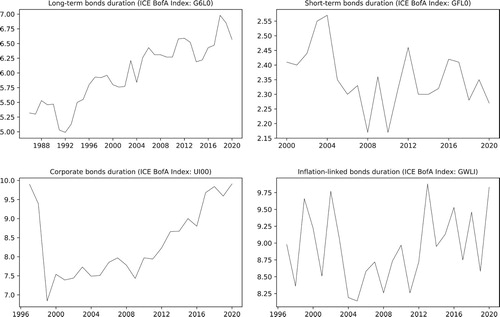
Table 7. Duration of bond portfolios, based on the end-of-year values recorded in 2019 for the ICE BofA indices mentioned in Section 5.1.

Portfolio	Duration
Short-term bonds	2.27
Long-term bonds	6.57
Inflation-linked bonds	9.83
Corporate bonds	9.91

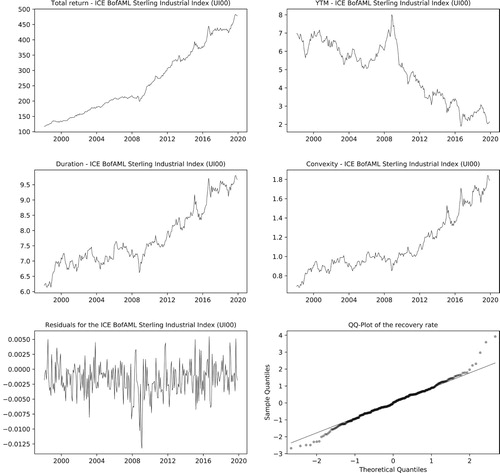
5.3.3. Corporate bonds

In the case of corporate bonds, the effect of default losses is represented by the term $\mathrm{\Delta }\ln I$ in (4(4) $\mathrm{\Delta }\ln P\approx Y_t\mathrm{\Delta }t-D_t\mathrm{\Delta }Y+\mathrm{\Delta }\ln I,$(4) ). Historical values for the recovery rates can be computed by $\mathrm{\Delta }\ln I\approx \mathrm{\Delta }\ln P-Y_t\mathrm{\Delta }t+D_t\mathrm{\Delta }Y$from historical prices, yields and durations, as shown in Section 2.2; see Figure 7. The values for the historical recovery rates are mostly negative. We will model the recovery index as iid random variables with $\ln (-\mathrm{\Delta }\ln I+\delta )\sim N(\mu ,{\sigma }^2).$The qq-plot in Figure 7 shows the adherence of the recovery rates to the log-normal model. With a shift $\delta =0.1$, the maximum likelihood estimators for the mean μ and variance ${\sigma }^2$ are respectively equal to $-2.29$ and 7.47e−4.

Figure 7. The four topmost pictures illustrate the historical data used in the calibration of corporate bonds. The residuals used to estimate the recovery rate are illustrated in the bottom left picture. Next to it, the QQ-plot illustrating their good adherence to the lognormal model.

5.3.4. User views

For the experiments in Section 6, short-term forecasts and long-term views on the median values of the risk factors are specified in accordance with the ‘Long-term economic determinants’ (Office for Budget Responsibility 2020b) published by the UK's Office for Budget Responsibility (OBR). The publication contains yearly forecasts for macroeconomic variables in the period between 2020 and 2070. We adopt the OBR's forecasts for the first five years (2020–2024) as our short-term forecasts and the 2070 forecasts as our long-term views; see Table 8.

Table 8. Short-term forecasts and long-term views used in the model. Yearly percentage change values from the long-term economic determinants published by the Office for Budget Responsibility (OBR).

	Short-term forecasts
Year	2020	2021	2022	2023	2024	Long-term views 2070
Nominal GDP growth (%)	3.0	3.3	3.9	3.5	3.4	3.9
Average earnings growth (%)	2.9	3.6	3.3	3.5	3.0	3.8
CPI inflation (%)	1.8	1.4	1.9	2.1	2.0	2.0
Long-term yields (%)	0.8	0.9	0.9	0.9	1.0	4.1
Short-term yields (%)	0.8	0.8	0.8	0.8	0.8	4.1

In order to apply Proposition 4.1, as described in Section 4.2, we write the autoregression matrix A from Table 4 as $A=\alpha \text{β}$, where the matrices α and β are given in Table 9(a,b), respectively. The eigenvalues of the matrix $I+\text{β}\alpha$ are $\lambda (I+\text{β}\alpha )=\{0.840,0.867,0.838,0.678,0.338,0.588,0.407,0.387,0.843,0.898\}$which are all real and of modulus strictly less than one. Proposition 4.1 then says that the long run means of $\text{β}x$ and $\mathrm{\Delta }x$ will be given by the vectors c and d, respectively, provided $\text{β}d=0$. Recall that, without this latter condition, the long-term mean of $\text{β}x$ cannot exist if x is to have long-term mean drift d.

Table 9. Decomposition of the autoregression matrix: $A=\alpha \text{β}$.

(a) Matrix α
I	−0.161409
G		−0.592506
E		0.429563
S
$Y^s$	1.015025	2.882123	−0.159839
$Y^l$	0.900122	1.756314		−0.132922
C		-3.642201			−0.661356
$\hat{I}$						−0.612425
$v^{1,m}$							−0.156411
$v^{2,m}$
$v^{3,m}$									1.0
$v^{1,f}$								−0.101227
$v^{2,f}$
$v^{3,f}$										1.0
(b) Matrix β
I	G	E	S	$Y^s$	$Y^l$	C	$\hat{I}$	$v^{1,m}$	$v^{2,m}$	$v^{3,m}$	$v^{1,f}$	$v^{2,f}$	$v^{3,f}$
1.0
	1.0
				1.0
					1.0
						1.0
							1.0
								1.0
											1.0
		0.055879								−0.32163
		0.160821											−0.411197

The choice of β in Table 9 implies that the components of c will specify the long-term means of I, G, $Y^s$, $Y^l$, C, $\hat{I}$, $v^{1,m}$, $v^{1,f}$ as well as the linear combinations of $v^{3,m}$ and $v^{3,f}$ with E; see Table 3 for the definitions of the risk factors. As described in Remark 4.1, the components of c corresponding to I, G, $Y^s$ and $Y^l$ are obtained by passing the long-term views in Table 8 through the nonlinear transformations given in Table 3. The long-term mean of the inflation expectation spread $\hat{I}$ was set equal to zero while the mean of C as well as those of the cointegration vectors in the last two rows of β were set equal to their historical means. The long-term means of $v^{1,m}$ and $v^{1,f}$ were chosen to match the regression intercepts. The resulting vector c is given in Table 10(a).

Table 10. Specification of long-term views using the vectors c of long-term means of $\text{β}{x}_t$ and d of long-term means of $\mathrm{\Delta }{x}_t$.

(a) Vector c
I	G	C	$\hat{I}$	$Y^s$	$Y^l$	$v^{1,m}$	$v^{1,f}$	${\text{β}}_{9}x$	${\text{β}}_{10}x$
0.045940	0.027831	−3.850433	0	−2.287811	−2.234210	8.113048	8.649000	0.222964	0.314955
(b) Vector d
	I	G	E	S	$Y^s$	$Y^l$	C	$\hat{I}$	$v^{1,m}$	$v^{2,m}$	$v^{3,m}$	$v^{1,f}$	$v^{2,f}$	$v^{3,f}$
	0	0	0.021612	0.105269	0	0	0	0	0	0.017694	0.007068	0	0.016597	0.010647

Note: Above, ${\text{β}}_i$ is the ith row of β.

As to the vector d of long-term expected drifts, we start by setting the components corresponding to the stationary variables equal to zero. The drift of the earnings is set according to Table 8. The drifts of $v^{3,m}$ and $v^{3,f}$ are then given uniquely by the condition $\text{β}d=0$. The long-term mean drifts of the logarithmic stock index and the longevity risk factors $v^{2,m}$ and $v^{2,f}$ were set to match their historical mean drifts. The resulting vector d is given in Table 10(b). We have $\text{β}d=0$ so all the conditions of Proposition 4.1 are satisfied.

We emphasize that the above choices of c and d should be only taken as an illustration of the use of the model. In a given application, the user of the model is free to specify the views and forecasts according to their own best judgement.

6. Simulation results

In this section, we use the calibrated time series model in a simulation experiment. First, we use the time series model to generate scenarios for the risk factors x. After that, we apply the inverses of the transformations presented in Section 5.2. Simulation results for 500k scenarios and a time horizon of 70 years are illustrated in Figures 8 and 9. The figures plot the historical data and the median of the simulated scenarios with 95% and 99% confidence bands and a single-simulated scenario.

Figure 8. Simulated scenarios for the economic and financial risk factors. The plots show the historical risk factors with a single-simulated scenario and the 95% and 99% confidence bands.

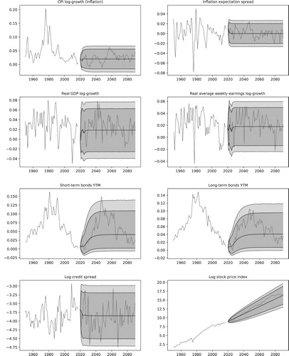
Figure 9. Simulated scenarios for the survival probabilities of the 18, 65 and 105 year-old cohorts. The plots show the historical probabilities with a single simulated scenario and the 95% and 99% confidence bands.

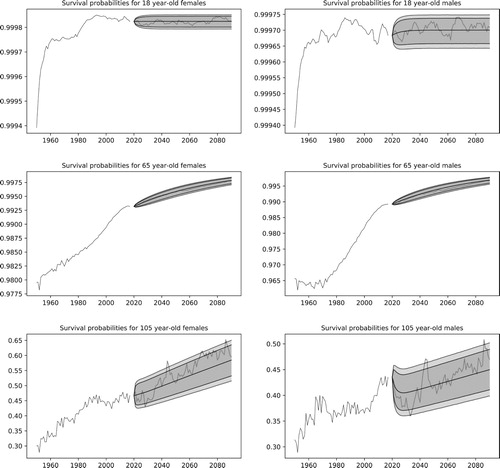
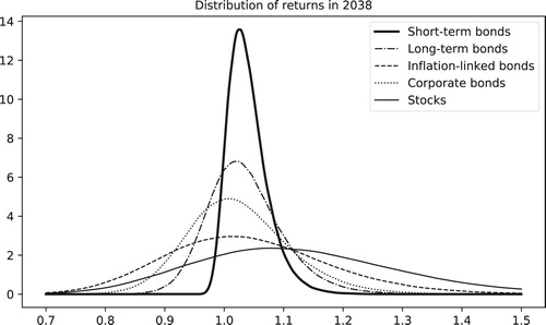
In the simulation results, one can observe the convergence of the medians to the values specified in Section 5.3.4. In addition, the mean-reverting characteristic of the yields, spreads and the log-growths of CPI, AWE and GDP can be visually confirmed by the horizontal confidence bands. Finally, as described in Section 5.3.1, the model has been calibrated to reflect the recent behavior of inflation, which does not present the volatility levels observed in the 80s. In line with the results previously shown in Aro & Pennanen (2011) and Glover (2018), one notices that the survival probabilities for the 18-year-old cohorts has already reached an equilibrium level and now presents mean-reverting behavior. The probabilities for the older cohorts, however, are still improving; See Figure 9. Figure 10 shows kernel density plots for the distribution of returns in each asset class in the year 2038. As one would expect, the short-term bonds present the smallest variance, long-term bonds the second largest, and stocks the largest.

Figure 10. The picture illustrates the distribution of the asset returns for a specific year using density plots.

6.1. Computation times

Our calibration and simulation programs were implemented in Python 3.7. Using an AMD Ryzen Threadripper 1950x 16-core processor with 128 GB of RAM (now a three year-old system) running Linux, the calibration of the model to historical data takes on average 0.34 s. The fast calibration time is not surprising, as it consists in estimating the coefficients of the A matrix using linear regression and the covariance matrix Σ using the regression residuals. However, as described in Section 4.1, specifying the structure of the model is an iterative procedure involving statistical analysis and a certain degree of economic expertize.

Simulation times obtained using the same system can be found in Table 11. The current implementation generates half a million scenarios in less than 1 min and one million scenarios in approximately 90 s. The figures show that about half of the time is spent on the simulation of the risk factors and the other half on the computation of the asset returns, where most of the time is spent with the returns on portfolios of corporate bonds, which involve the idiosyncratic default risk; See Section 5.3.3. Even though the code is not fully optimized, it already shows the benefits of our approach, where a reduced number of risk factors is used for the survival probabilities and returns on bond portfolios.

Table 11. Computation times in seconds for the simulation of risk factors.

Scenarios	Total	Simulation of risk factors	Returns	Returns on corporate bonds
100k	9.84	5.20	4.02	3.51
200k	18.60	9.33	8.06	7.07
300k	27.38	13.49	12.09	10.60
400k	36.19	17.76	16.03	14.03
500k	45.21	22.04	20.14	17.66
600k	54.11	26.17	24.29	21.28
700k	62.44	30.43	27.91	24.56
800k	71.30	34.69	31.88	28.03
900k	78.86	38.87	34.88	30.64
1000k	88.61	42.95	39.79	34.98

6.2. Population sizes

As a first step to the computation of pension payments, we study the dynamics of a population using the models presented in Section 2.1, in which Binomial random variables are used to track the total number of survivors from one year to the next, with survival probabilities that are based on the simulated mortality risk factors. Simulation results for 500k scenarios for cohorts of 18 and 85 year-old females of size 10, 100 and 1000 are illustrated in Figure 11. In each plot, median values and the 95% and 99% confidence bands for the population size are shown. Simulations stopped when all individuals died.

Figure 11. Simulation of population sizes with survival probabilities from the UK model. Plots on the left show the median values of the population size with the 95% and 99% confidence bands for cohorts of 18-year-old females with sizes 10, 100 and 1000. Results for 85-year-old females are shown on the right. The top plots clearly illustrate the discrete nature of the Binomial random variables used to model the population sizes.

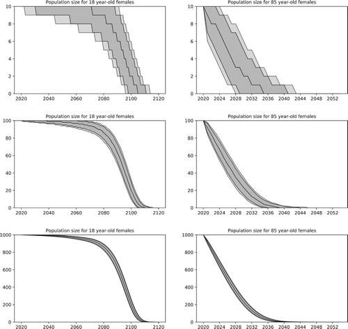
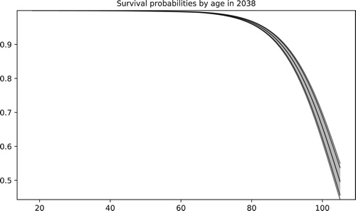
Inspecting the results, one can notice the different shapes of the curves obtained for the 18 and 85 year-old cohorts. For the younger cohort, the population size decreases slowly at first and then accelerates its decrease as the population ages. In the simulations, the change happens around the year 2070, when the individuals reach their 70s. For the older cohort, we find that the population size decreases rapidly. Unsurprisingly, these observations are understood when one looks into the survival probabilities for all ages at a specific point in time. As shown in Figure 12, survival probabilities remain fairly high until the age of 70 and rapidly decrease after that.

Figure 12. The picture illustrates the median, the 95% and 99% confidence bands for the survival probabilities of females in a specific year.

The results also show a wide confidence interval for the times in which the population size becomes zero. These are particularly important for pension fund managers as they mark the end of all pension liabilities and also the investment horizon. For the smaller cohort of 85-year-old females, for example, in 95% of the scenarios all individuals seem to die within a period of 12 years, between 2029 and 2041. Moreover, the results show that larger populations will outlive smaller ones on average. This is particularly clear when comparing the medians of population sizes for the older cohort. For example, the median size for the smaller 85-year-old cohort is zero in the year 2035, but the same value is not reached before 2039 for the larger cohorts. The result is easy to understand, as one of the factors used in the computation of medians for Binomial random variables is the number of trials, which corresponds here to the population size.

6.3. Pension payments

We now study payments in the context of defined benefit (DB) pension schemes, which are characterized by guaranteed benefits that are periodically adjusted in accordance to an index, typically inflation. 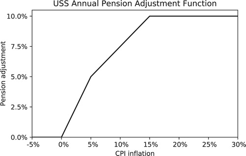At time t, the total pension payment to a population $B_t$ of pensioners is given by (12) $c_t=\sum _{b\in B_t}{F}_t{c}_0^b,$(12) where $c_0^b$ is the initial benefit paid to a pensioner and $F_t$ an adjustment factor that is regularly updated. Considering annual adjustments that are based on inflation, as measured by the CPI, we assume that the adjustment factor is given by (13) $F_t=\prod _{k=0}^t\left[1+f_{adj}\left(\frac{{\mathrm{C}\mathrm{P}\mathrm{I}}_k-{\mathrm{C}\mathrm{P}\mathrm{I}}_{k-1}}{{\mathrm{C}\mathrm{P}\mathrm{I}}_{k-1}}\right)\right],$(13) for an adjustment function $f_{adj}$ that is specific to each pension scheme. As an example, the adjustment function adopted by the Universities Superannuation Scheme (USS) is illustrated in Figure 13.

Figure 13. Benefit adjustment function adopted by the Universities Superannuation Scheme (USS). As illustrated, no adjustments are made in the case of negative inflation, and only partial adjustments are offered for high inflation.

Under the specifications above, one can easily identify the main sources of risk affecting pensions: indexation and longevity. In order to quantify the contribution of each risk factor to the overall financial risk, we compute the pension payments removing risk factors one at a time, replacing them by their median values. This approach leads to four different computations, as illustrated in Figure 14, where the payments made to a group of 100 sixty-five-year-old female pensioners are shown. To better represent the purchasing power of individuals, we express pension payments in real terms (i.e. $\frac{c_t}{{\mathrm{C}\mathrm{P}\mathrm{I}}_t}$).

Figure 14. Illustration of the effects of indexation risk and longevity risk on pension payments expressed in real terms. In the top left, both are fixed to their median values. In the top right, inflation is fixed. Bottom left, longevity is fixed. Bottom right, both are stochastic.

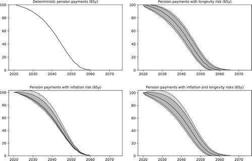
The top-left plot in Figure 14 shows a deterministic projection of the future payments, computed with constant inflation at 2% and median population sizes. In the top-right plot, the effects of the longevity risk are included, as simulated survival probabilities are used to control the population sizes while maintaining inflation constant at 2%. The bottom-left plot illustrates the inflation risk, as payments are adjusted in accordance to the USS regulations. Finally, the bottom-right plot shows the joint effects of the inflation and longevity risks, as no deterministic replacements are in place.

The results show that inflation risk is dominant in the first years of the simulation, when the population sizes are usually larger, and that the longevity risk seems to play a larger role in the long run, as illustrated by the larger confidence bands found when it is present. Another interesting feature in the results is the growth of the pension payments in real terms, observed when in the inflation risk is present. Such growth corresponds to periods of negative inflation, and is a direct result of the USS pension adjustments. As shown in Figure 13, payments are not decreased when inflation is negative.

6.4. Longevity and economic growth

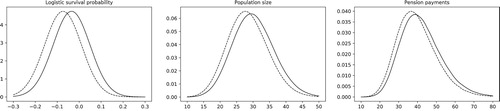
Evidence of the link between old-age longevity and economic growth has already been presented in Aro & Pennanen (2014) and Glover (2018) and references therein. In our model, as in Glover (2018), the mortality risk factors associated with the longevity of the elderly are linked to economic growth through the real AWE. This link is tested here by replacing the 2024 nominal GDP growth forecast in Table 8 with a 10% drop and examining the impact on the cohort of 1000 eighty-five-year-old female pensioners. Simulation results, illustrated in Figure 15, show a decrease in the survival probabilities of the elderly (represented by the risk factor $v^{3,f}$) which, in turn, cause an decrease in the population sizes and the associated pension payments.

Figure 15. The leftmost picture shows the distribution of the risk factor $v^{3,f}$ in 2035. The center plot shows, at the end of the same year, the distribution of population sizes for a cohort that had one thousand 85 year-old females in 2020. Corresponding pension payments are shown in the rightmost plot. Dashed lines show the impact of a 10% reduction in GDP in 2024.

6.5. ALM study of a closed DB fund

We now focus on the asset-liability management of a closed DB fund, that is, a scheme that is closed to new members and to accrual of new benefits. According to the estimates provided in the ‘Purple Book’ (Pension Protection Fund 2019), closed funds correspond to 41% of the 5436 DB-funds in the UK that are eligible for protection from the Pension Protection Fund (PPF).

More specifically, we consider a pension scheme with the liabilities described in Section 6.3 and 200k in assets. We generate 500k scenarios 70 years into the future and, in each scenario, we calculate the fund wealth at the end of each year after collecting the investment returns and paying out the pension benefits. At the beginning of each year, the remaining wealth is reallocated among the available asset classes in fixed proportions. Thus, in each scenario, the wealth at the beginning of year t is given by $w_t=\sum _{j\in J}{r}_t^j{h}_{t-1}^j-c_t,$where $c_t$ is the pension expenditure, J is the set of traded assets, $h_t^j$ is the amount of wealth invested in asset $j\in J$ at the beginning of year t and $r_t^j$ is the return per unit of wealth invested. In each scenario, the investment strategy h is updated yearly according to $h_t^j={\pi }^j{w}_t,$where ${\pi }^j$, $j\in J$, are prespecified proportions. If wealth w becomes negative, we assume that the remaining pension payments are financed by borrowing from the money market.

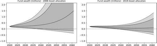
The proportions used in rebalancing are based on the 2008 and 2019 average asset allocations in Tables 1 and 2, which have been adjusted to compensate for the asset classes that are not available in our models (e.g. property, hedge funds, etc.). The 2008 and 2019 allocations have been chosen for illustrating how the investment strategies adopted by pension funds in the UK have changed after the financial crisis of 2008. Before the crisis, funds used to invest 53.6% of its wealth in equities and 32.9% in bonds. At the moment, average investments are at 24.0% in equities and 62.8% in bonds.

The development of the wealth processes w corresponding to the two rebalancing strategies are illustrated in Figure 16. As one would expect, the higher proportion of stocks in the 2008 allocation results in wider distribution for the net wealth. It would be natural to try to optimize the investment strategy by minimizing a given performance criterion over all feasible strategies that are adapted to the information available to the fund managers over time. Preliminary results in that direction were obtained in (Hilli et al. 2011) for the case without longevity risk. Extensions to the general setting will be explored in a subsequent paper.

Figure 16. The plots compare simulations for the wealth of a pension fund using the 2008 and 2019 average asset allocations from Tables 1 and 2. In the most recent allocation, over 60% of the funds are invested in bonds, resulting in lower risks, but also in lower gains on average, as illustrated by the median of the wealth in the plots. The 95% and 99% quantiles are also illustrated in the plots.

6.6. A study of the impact of the COVID-19 pandemic

Building on the previous simulation studies, we now focus on the impact of the COVID-19 pandemic on a closed DB fund that supports a cohort of 100 85 year-old females. We investigate the annual developments of its pension payments and wealth under pre- and post-COVID-19 views.

The pre-COVID-19 baseline is represented by the OBR's ‘Long-term economic determinants’ (LTD) (Office for Budget Responsibility 2020b), from which we obtained the short-term forecasts and long-term views used in the calibration of our model, as described in Section 4.2. Assuming the pandemic produces a short-term effect on longevity and on the economy, as suggested by Cairns et al. (2020) and by the economic forecasts published by the OBR and by the Bank of England's Monetary Policy Committee (Bank of England's Monetary Policy Committee 2020), we build the post-COVID-19 views by combining the long-term views of the LTD with short-term forecasts that contain both economic and longevity shocks. On the economic side, we adopt the shocks described in the OBR's ‘Coronavirus analysis’ (Office for Budget Responsibility 2020a), which can be found in Table 12.

Table 12. Short-term forecasts used in the COVID-19 impact study to model the economic impact of the pandemic, based on the Office for Budget Responsibility's Coronavirus reference scenario.

	Short-term forecasts (post-COVID-19)
Year	2020	2021	2022	2023	2024
Nominal GDP growth (%)	−12.8	17.9	1.5	1.3	1.4
CPI inflation (%)	1.2	2.3	2.4	2.3	2.2
Average earnings growth (%)	−7.3	18.3	1.6	2.5	3.1
Short-term yields (%)	0.1	0.2	0.3	0.3	0.3
Stock index growth (%)	−9.5	16.1	8.6	4.3	3.6

According to Milevsky (2020), preliminary results indicate that COVID-19 has caused a parallel shift in the mortality rates associated with retirement ages. Accordingly, we shift the longevity risk factors of Section 2.1 so that all mortality rates in 2020 and 2021 are increased by a factor that corresponds to a 4-year increase of age, producing a longevity shock similar to the one estimated in Cairns et al. (2020).

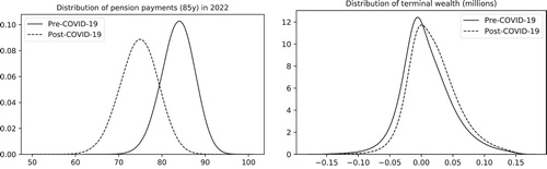
Simulation results with the pre- and post-COVID-19 views can be found in Figures 17 and 18. The top row of Figure 17 illustrates the development of the yearly pension expenditure for the fund, while the bottom row plots the development of the remaining asset values. Figure 18 provides kernel density plots for the distribution of pension payments in 2022 and for the terminal wealth. While the economic shock lowers the asset values in the short term, the increased mortality rates lower the pensions expenditure so that the distribution of the terminal wealth improved under the post-COVID-19 view.

Figure 17. The plots compare pension payments in real terms and remaining asset value in the pre- and post-COVID-19 settings, as described in Section 6.6. Liabilities correspond to a cohort of 100 85 year-old females. The median and the 95% and 99% quantiles are illustrated in the plots.

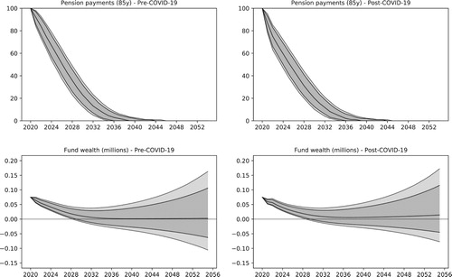
Figure 18. Kernel density plots for the distribution of pension payments in 2022 and for the terminal wealth of the DB fund under pre- and post-COVID-19 views.

Disclosure statement

No potential conflict of interest was reported by the authors.

Additional information

Funding

Research partially supported by the Pensions Policy Institute

References

- Actuarial Post (2019). Impact of negative real yields on UK pension schemes. Available at: http://tiny.cc/zibgiz.
- Allsopp C., Kara A. & Nelson E. (2006). United kingdom inflation targeting and the exchange rate. The Economic Journal 116(512), F232–F244. doi: https://doi.org/10.1111/j.1468-0297.2006.01098.x
- Armstrong J., Carrera L., Pennanen T. & Redwood D. (2013). Automatic enrollment report 1: What level of pension contribution is needed to obtain an adequate retirement income? Available at:http://tiny.cc/iwpwjz.
- Aro H. & Pennanen T. (2011). A user-friendly approach to stochastic mortality modelling. European Actuarial Journal 1(2), 151–167. doi: https://doi.org/10.1007/s13385-011-0030-4
- Aro H. & Pennanen T. (2014). Stochastic modelling of mortality and financial markets. Scandinavian Actuarial Journal 2014(6), 483–509. doi: https://doi.org/10.1080/03461238.2012.724442
- Bank of England's Monetary Policy Committee (2020). Monetary policy report. Available at: http://tiny.cc/aabvqz.
- Bjornland H. C. (2000). Var models in macroeconomic research. Available at:http://tiny.cc/m3ryty.
- Black F. & Karasinski P. (1991). Bond and option pricing when short rates are lognormal. Financial Analysts Journal 47(4), 52–59. doi: https://doi.org/10.2469/faj.v47.n4.52
- Box G. E. P. & Cox D. R. (1964). An analysis of transformations. Journal of the Royal Statistical Society: Series B (Methodological) 26(2), 211–243.
- Cairns A. J. G., Blake D., Dowd K., Coughlan G. D., Epstein D. & Khalaf-Allah M. (2011). Mortality density forecasts: an analysis of six stochastic mortality models. Insurance: Mathematics and Economics 48(3), 355–367.
- Cairns A. J. G., Blake D. P., Kessler A. & Kessler M. (2020). The impact of covid-19 on future higher-age mortality. Available at: SSRN 3606988.
- Canova F. (1999). Vector Autoregressive Models: Specification, Estimation, Inference, and Forecasting. In Handbook of Applied Econometrics Volume 1: Macroeconomics, edited by H. Pesaran, and P. Schmidt, John Wiley & Sons, Ltd.
- Engle R. F. & Granger C. W. J. (1987). Co-integration and error correction: representation, estimation, and testing. Econometrica: Journal of the Econometric Society 55(2), 251–276. doi: https://doi.org/10.2307/1913236
- Financial Times (2020). Negative yields: Getting to grips with the great bond rally. Available at: http://tiny.cc/849fiz.
- Glover M. H. (2018). Trends in the UK mortality experience. MPhil Dissertation, King's College London.
- Hamilton J. D. A. (1994). Time series analysis. Princeton, NJ: Princeton University Press.
- Hilli P., Koivu M. & Pennanen T. (2011). Optimal construction of a fund of funds. European Actuarial Journal 1(2), 345–359. doi: https://doi.org/10.1007/s13385-011-0029-x
- Huber P. P. (1997). A review of wilkie's stochastic asset model. British Actuarial Journal 3(1), 181–210. doi: https://doi.org/10.1017/S1357321700005328
- Hunt A. & Blake D. (2014). A general procedure for constructing mortality models. North American Actuarial Journal 18(1), 116–138. doi: https://doi.org/10.1080/10920277.2013.852963
- Intercontinental Exchange (2019). ICE Index Platform. Available at: https://indices.theice.com.
- Koivu M. & Pennanen T. (2014). Return dynamics of index-linked bond portfolios. The Journal of Portfolio Management 41(1), 78–84. doi: https://doi.org/10.3905/jpm.2014.41.1.078
- Koivu M., Pennanen T. & Ranne A. (2005a). Modeling assets and liabilities of a Finnish pension insurance company: a VEqC approach. Scandinavian Actuarial Journal 2005(1), 46–76. doi: https://doi.org/10.1080/03461230510009709
- Koivu M., Pennanen T. & Ziemba W. T. (2005b). Cointegration analysis of the Fed model. Finance Research Letters 2(4), 248–259. doi: https://doi.org/10.1016/j.frl.2005.06.002
- Lee R. D. & Carter L. R. (1992). Modeling and forecasting US mortality. Journal of the American Statistical Association 87(419), 659–671.
- Lütkepohl H. (2005). New introduction to multiple time series analysis. Berlin: Springer-Verlag.
- Milevsky M. (2020). Is COVID-19 a parallel shock to the term structure of mortality? Available at: http://tiny.cc/71bvqz.
- Moll T. (2019). Just say no to negative real yields. Available at: http://tiny.cc/cbbgiz.
- Mulvey J. M. (1996). Generating scenarios for the towers Perrin investment system. Interfaces 26(2), 1–15. doi: https://doi.org/10.1287/inte.26.2.1
- Mulvey J. M. & Thorlacius A. E. (1998). The towers perrin global capital market scenario generation system. Worldwide Asset and Liability Modeling 10, 286.
- Office for Budget Responsibility (2020a). Coronavirus analysis. Available at: https://obr.uk/coronavirus-analysis/.
- Office for Budget Responsibility (2020b). Long-term economic determinants. Available at: https://obr.uk/efo/economic-and-fiscal-outlook-march-2020/.
- Pension Protection Fund (2019). The purple book. Available at: https://www.ppf.co.uk/purple-book.
- Sims C. A. (1980). Macroeconomics and reality. Econometrica: Journal of the Econometric Society 48(1), 1–48. doi: https://doi.org/10.2307/1912017
- Thomas R. & Dimsdale N. (2017). A millennium of UK data. Available at: https://www.bankofengland.co.uk/statistics/research-datasets.
- University of California, Berkeley (USA), and Max Planck Institute for Demographic Research (Germany), Human mortality database. Available at: www.mortality.org.
- Van der Weide R. (2002). Go-garch: a multivariate generalized orthogonal garch model. Journal of Applied Econometrics 17(5), 549–564. doi: https://doi.org/10.1002/jae.688
- Wilkie A. D. (1984). A stochastic investment model for actuarial use. Transactions of the Faculty of Actuaries 39, 341–403. doi: https://doi.org/10.1017/S0071368600009009
- Wilkie A. D. (1995). More on a stochastic asset model for actuarial use. British Actuarial Journal 1(5), 777–964. doi: https://doi.org/10.1017/S1357321700001331
- Wilkie A. D. & Sahin S. (2016). Yet more on a stochastic economic model: part 2: initial conditions, select periods and neutralising parameters. Annals of Actuarial Science 10(1), 1–51. doi: https://doi.org/10.1017/S174849951500010X
- Wilkie A. D. & Sahin S. (2019). Yet more on a stochastic economic model: part 5: a vector autoregressive (var) model for retail prices and wages. Annals of Actuarial Science 13(1), 92–108. doi: https://doi.org/10.1017/S1748499518000106
- Wilkie A. D., Sahin S., Cairns A. J. G. & Kleinow T. (2011). Yet more on a stochastic economic model: part 1: updating and refitting, 1995 to 2009. Annals of Actuarial Science 5(1), 53–99. doi: https://doi.org/10.1017/S1748499510000072
- Yeo I. & Johnson R. A. (2000). A new family of power transformations to improve normality or symmetry. Biometrika 87(4), 954–959. doi: https://doi.org/10.1093/biomet/87.4.954