LocalGLMnet: interpretable deep learning for tabular data

ABSTRACT

Deep learning models have gained great popularity in statistical modeling because they lead to very competitive regression models, often outperforming classical statistical models such as generalized linear models. The disadvantage of deep learning models is that their solutions are difficult to interpret and explain, and variable selection is not easily possible because deep learning models solve feature engineering and variable selection internally in a nontransparent way. Inspired by the appealing structure of generalized linear models, we propose a new network architecture that shares similar features as generalized linear models but provides superior predictive power benefiting from the art of representation learning. This new architecture allows for variable selection of tabular data and for interpretation of the calibrated deep learning model, in fact, our approach provides an additive decomposition that can be related to other model interpretability techniques.

KEYWORDS:

• Deep learning
• neural network
• generalized linear model
• regression model
• variable selection
• explainable deep learning
• attention layer
• tabular data
• exponential dispersion family
• model interpretability

1. Introduction

Deep learning models celebrate great success in statistical modeling because they often provide superior predictive power over classical regression models. This success is based on the fact that deep learning models perform representation learning of features, which means that they bring features into the right structure to be able to extract maximal information for the prediction task at hand. This feature engineering is done internally in a nontransparent way by the deep learning model. For this reason, deep learning solutions are often criticized to be non-explainable and interpretable, in particular, because this process of representation learning is performed in high-dimensional spaces analyzing bits and pieces of the feature information. Recent research has been focusing on interpreting machine learning predictions in retrospect, see, e.g. Friedman's partial dependence plot (PDP) (Friedman 2001), the accumulated local effects (ALE) method of Apley & Zhu (2020), the locally interpretable model-agnostic explanation (LIME) introduced by Ribeiro et al. (2016), the SHapley Additive exPlanations (SHAP) of Lundberg & Lee (2017) or the marginal attribution by conditioning on quantiles (MACQ) method proposed by Merz et al. (2022). PDP, ALE, LIME and SHAP can be used for any machine learning method such as random forests, boosting or neural networks, whereas MACQ requires differentiability of the regression function which is the case for neural networks under differentiable activation functions; for a review of more gradient-based methods, we refer to Merz et al. (2022).

We follow a different approach here, namely, we propose a new network architecture that has an internal structure that directly allows for interpreting and explaining. Moreover, this internal structure also allows for variable selection of tabular feature data and to extract interactions between feature components. The starting point of our proposal is the framework of generalized linear models (GLMs) introduced by Nelder & Wedderburn (1972) and McCullagh & Nelder (1983). GLMs are characterized by the choice of a link function that maps the regression function to a linear predictor, and, thus, leading to a linear functional form that directly describes the influence of each predictor variable on the response variable. Of course, this (generalized) linear form is both transparent and interpretable. To some extent, our architecture preserves this linear structure of GLMs, but we make the coefficients of the linear predictors feature dependent. Such an approach follows a similar strategy as the ResNet proposal of He et al. (2016) that considers a linear term and then builds the network around this linear term. The LassoNet of Lemhadri et al. (2021) follows a similar philosophy, too, by performing Lasso regularization on network features. Both proposals have in common that they use a so-called skip connection in the network architecture that gives a linear model part around which the non-linear network model is built. Our proposal uses such a skip connection, too, which provides the linear model part, and we weight these linear terms with potentially non-linear weights. This allows us to generate non-linear regression functions with arbitrary interactions. In spirit, our non-linear weights are similar to the attention layers recently introduced by Bahdanau et al. (2014) and Vaswani et al. (2017). Attention layers are a rather successful new way of building powerful networks by extracting more important feature components from embeddings by giving more weight (attention) to them. From this viewpoint we construct (network regression) attention weights that provide us with a local GLM for tabular data, and we therefore call our proposal LocalGLMnet. These regression attention weights also provide us with a possibility of explicit variable selection, which is a novel and unique property within network regression models. Moreover, we can explicitly explore interactions between feature components. A similar approach is considered in Ahn et al. (2021) on Bayesian credibility theory, where the credibility weights are modeled by attention weights.

There is another stream of literature that tries to choose regression structures that have interpretable features, e.g. the explainable neural networks (xNN) and the neural additive models (NAM) make restrictions to the structure of the network regression function by running different subsets of feature components through (separated) parallel networks, see Vaughan et al. (2018) and Agarwal et al. (2020). The drawback of these proposals is that representation learning is restricted within the parallel networks. Our proposal overcomes this issue as it allows for general interactions. We also mention (Richman 2021) who extends the xNN approach by explicitly including linear features to a combined model called CAXNN. Another interpretable network approach is the TabNet proposal of Arik & Pfister (2019). TabNet uses networks to create attention to important features for the regression task at hand, however, this proposal has the drawback that it may lead to heavy computational burden.

Our LocalGLMnet approach overcomes the limitations of these explainable network approaches. As we will see below, our proposal is computationally efficient and it leads to nice explanations, in the sense that we can interpret the predictions made by our model in terms of an additive decomposition of the features. This will be further explored in Section 2.4.

Our proposal of the LocalGLMnet, which estimates the coefficients of a (local) GLM, and, therefore, maintains a directly interpretable structure in terms of the original features, is, to the best of our knowledge, unique within the literature. In this key respect, the LocalGLMnet is different from the DeepGLM and the DeepGLMM of Tran et al. (2020), who study GLMs and generalized linear mixed models (GLMMs) that rely on learned feature representations from a deep neural network, i.e. the original features are not used directly to make predictions. One similarity between these model approaches is that the DeepGLMM allows for observation specific random effects in the last layer of that model, thus, the coefficients may vary for each observation, which is similar to our LocalGLMnet. Whereas the LocalGLMnet complies with the interpretable machine learning requirements discussed in the manifesto of Rudin (2019), the interpretable models discussed in that work and its references rely on significantly different classes of algorithms from GLMs, which we focus on here due to the importance of GLMs within actuarial work. Among the models mentioned in Rudin (2019), perhaps the most similar is the prototype network of Chen et al. (2019), which performs classification based on the similarity of an image to interpretable learned prototypes, which are used as interpretable features within a deep neural network. In the case of the LocalGLMnet, the original feature values are used directly to make predictions, thus, maintaining interpretability. Within the machine learning literature, the most similar work to the LocalGLMnet is the hypernetwork concept of Ha et al. (2016), where one neural network is used to estimate the weights of a second network. In the case of the LocalGLMnet, a neural network is being used to estimate the weights of a second model, which is a (local) GLM. Similar types of models have been considered within the actuarial literature in the context of mortality forecasting by, e.g. Perla et al. (2021), who derive the coefficients of a Lee–Carter type of model using convolutional and recurrent neural networks.

Using the LocalGLMnet architecture, we propose an empirically based Wald-type method for variable selection, which relies on adding synthetic variables generated by a uniform or Gaussian distribution to the data before the LocalGLMnet is fitted. The estimated non-linear regression weights for these synthetic variables are then used to estimate a confidence interval to determine the significance of the regression weights for the rest of the dataset. The method proposed here is closely connected to the Boruta system of variable selection proposed by Kursa & Rudnicki (2010), which functions by adding permuted copies of the features to a random forest algorithm, and assessing the significance of each feature with reference to the level of significance assigned to these permuted features by the variable importance scores within the random forest algorithm. The approach proposed here is similar in that synthetic variables are added to the dataset, but differs in terms of how the significance of the features is evaluated: as opposed to using variable importance scores, the structure of the LocalGLMnet allows for the significance of variables to be evaluated directly in terms of the regression weights.

1.1. Organization of this manuscript

In the next section, we introduce and discuss the LocalGLMnet. We therefore first recall the GLM framework which will give us the right starting point and intuition for the LocalGLMnet. In Section 2.2, we extend GLMs to feed-forward neural networks that form the basis of our regression attention weight construction, and Section 2.3 presents our LocalGLMnet proposal that combines GLMs with regression attention weights. Section 2.4 discusses the LocalGLMnet, and it relates our proposal to other methods. Section 3 presents two examples, a toy synthetic data example and a real data example. The former will give us a proof of concept, a verification is obtained because we know the true data generating mechanism in this toy synthetic data example. Moreover, in Section 3.2 we discuss how the LocalGLMnet allows for variable selection, which is a novel and unique property within network regression modeling. Section 3.3 explains how we can find interactions. In Section 3.4, we present the main demonstration of the LocalGLMnet on a real data example which has been studied extensively in recent actuarial work. In the context of this example, Section 3.5 discusses variable importance, and in Section 3.6 we discuss how categorical feature components can be treated within our proposal. Finally, in Section 4 we conclude, and in the appendix we provide further analysis.

2. Model architecture

2.1. Generalized linear model

The starting point of our proposal is a GLM which typically is based on the exponential dispersion family (EDF). GLMs have been introduced by Nelder & Wedderburn (1972) and McCullagh & Nelder (1983), and the EDF has been analyzed in detail by Jørgensen (1997) and Barndorff-Nielsen (2014); we use the notation and terminology of Wüthrich & Merz (2021), and for a detailed treatment of GLMs and the EDF we refer to Chapters 2 and 5 of that latter reference.

Assume we have a datum $(Y,\mathit{x},v)$ with a given exposure v>0, a vector-valued feature $\mathit{x}\in {\mathbb{R}}^q$, and a response variable Y following a member of the (single-parameter linear) EDF having density (w.r.t. to a σ-finite measure on $\mathbb{R}$) (1) $Y\sim f(y;\theta ,v/\phi )=\exp \{\frac{y\theta -\kappa \left(\theta \right)}{\phi /v}+a(y;v/\phi \left)\right\},$(1) with dispersion parameter $\phi >0$, canonical parameter $\theta \in \mathbf{\Theta }$, where the effective domain $\mathbf{\Theta }\subseteq \mathbb{R}$ is a non-empty interval, with cumulant function $\kappa :\mathbf{\Theta }\to \mathbb{R}$ and with normalizing function $a(\cdot ;\cdot )$. By construction of the EDF, the cumulant function κ is a smooth and convex function on the interior of the effective domain $\mathbf{\Theta }$. This implies that Y has first and second moments, we refer to Chapter 2 in Wüthrich & Merz (2021), $\mu =\mathbb{E}\left[Y\right]={\kappa }^{\prime }\left(\theta \right)\mathrm{a}\mathrm{n}\mathrm{d}\mathrm{V}\mathrm{a}\mathrm{r}\left(Y\right)=\frac{\phi }{v}{\kappa }^{″}\left(\theta \right)>0.$A GLM is obtained by making a specific regression assumption on the mean $\mu ={\kappa }^{\prime }\left(\theta \right)$ of Y. Namely, choose a strictly monotone and continuous link function $g:\mathbb{R}\to \mathbb{R}$ and assume that the mean of Y, given $\mathit{x}$, satisfies regression assumption (2) $\mathit{x}\mapsto g\left(\mu \right)=g\left(\mu \right(\mathit{x}\left)\right)={\text{β}}_0+〈\text{β},\mathit{x}〉={\text{β}}_0+\sum _{j=1}^q{\text{β}}_j{x}_j,$(2) with GLM regression parameter $\text{β}=({\text{β}}_1,\dots ,{\text{β}}_q{)}^{\mathrm{\top }}\in {\mathbb{R}}^q$, bias (intercept) ${\text{β}}_0\in \mathbb{R}$, and where $〈\cdot ,\cdot 〉$ denotes the scalar product in ${\mathbb{R}}^q$. This GLM assumption implies that the canonical parameter takes the following form (on the canonical scale of the EDF) $\theta =({\kappa }^{\prime }{)}^{-1}\left(g^{-1}({\text{β}}_0+〈\text{β},\mathit{x}〉)\right),$where $({\kappa }^{\prime }{)}^{-1}$ is called canonical link of the chosen EDF (1(1) $Y\sim f(y;\theta ,v/\phi )=\exp \{\frac{y\theta -\kappa \left(\theta \right)}{\phi /v}+a(y;v/\phi \left)\right\},$(1) ).

The GLM regression function (2(2) $\mathit{x}\mapsto g\left(\mu \right)=g\left(\mu \right(\mathit{x}\left)\right)={\text{β}}_0+〈\text{β},\mathit{x}〉={\text{β}}_0+\sum _{j=1}^q{\text{β}}_j{x}_j,$(2) ) is very appealing because it leads to a linear predictor $\eta \left(\mathit{x}\right)={\text{β}}_0+〈\text{β},\mathit{x}〉$ (after applying the link function g to the mean $\mu \left(\mathit{x}\right)$), and the regression parameter ${\text{β}}_j$ directly explains how the individual feature component $x_j$ influences the linear predictor $\eta \left(\mathit{x}\right)$ and the expected value $\mu \left(\mathit{x}\right)$ of Y, respectively. Our goal is to benefit from this transparent structure as far as possible.

2.2. Fully-connected feed-forward neural network

A neural network extension of a GLM is obtained rather easily by exploring feature engineering before considering the scalar product in the linear predictor (2(2) $\mathit{x}\mapsto g\left(\mu \right)=g\left(\mu \right(\mathit{x}\left)\right)={\text{β}}_0+〈\text{β},\mathit{x}〉={\text{β}}_0+\sum _{j=1}^q{\text{β}}_j{x}_j,$(2) ). A fully-connected feed-forward neural (FFN) network builds upon engineering feature information $\mathit{x}$ through non-linear transformations before entering the scalar product. A composition of FFN layers performs these non-linear transformations. Choose a non-linear activation function ${\varphi }_m:\mathbb{R}\to \mathbb{R}$ and dimensions $q_{m-1},q_m\in \mathbb{N}$. The mth FFN layer of a deep FFN network is defined by the mapping (3) $\begin{array}{rl}{\mathit{z}}^{\left(m\right)}:{\mathbb{R}}^{q_{m-1}}& \to {\mathbb{R}}^{q_m}\\ \mathit{x}& \mapsto {\mathit{z}}^{\left(m\right)}\left(\mathit{x}\right)={\left(z_1^{\left(m\right)}\right(\mathit{x}),\dots ,z_{q_m}^{\left(m\right)}(\mathit{x}\left)\right)}^{\mathrm{\top }},\end{array}$(3) having neurons $z_j^{\left(m\right)}\left(\mathit{x}\right)$, $1\le j\le q_m$, for variables $\mathit{x}=(x_1,\dots ,x_{q_{m-1}}{)}^{\mathrm{\top }}\in {\mathbb{R}}^{q_{m-1}}$, $z_j^{\left(m\right)}\left(\mathit{x}\right)={\varphi }_m(w_{0,j}^{\left(m\right)}+〈{\mathit{w}}_j^{\left(m\right)},\mathit{x}〉)={\varphi }_m(w_{0,j}^{\left(m\right)}+\sum _{l=1}^{q_{m-1}}{w}_{l,j}^{\left(m\right)}{x}_l),$for given network weights ${\mathit{w}}_j^{\left(m\right)}=(w_{l,j}^{\left(m\right)}{)}_{1\le l\le q_{m-1}}^{\mathrm{\top }}\in {\mathbb{R}}^{q_{m-1}}$ and bias $w_{0,j}^{\left(m\right)}\in \mathbb{R}$.

A FFN network of depth $d\in \mathbb{N}$ is obtained by composing d FFN layers (3(3) $\begin{array}{rl}{\mathit{z}}^{\left(m\right)}:{\mathbb{R}}^{q_{m-1}}& \to {\mathbb{R}}^{q_m}\\ \mathit{x}& \mapsto {\mathit{z}}^{\left(m\right)}\left(\mathit{x}\right)={\left(z_1^{\left(m\right)}\right(\mathit{x}),\dots ,z_{q_m}^{\left(m\right)}(\mathit{x}\left)\right)}^{\mathrm{\top }},\end{array}$(3) ) to provide a deep learned representation, we set input dimension $q_0=q$, (4) $\begin{array}{rl}{\mathit{z}}^{(d:1)}:{\mathbb{R}}^q& \to {\mathbb{R}}^{q_d}\\ \mathit{x}& \mapsto {\mathit{z}}^{(d:1)}\left(\mathit{x}\right)=({\mathit{z}}^{\left(d\right)}\circ \cdots \circ {\mathit{z}}^{\left(1\right)})\left(\mathit{x}\right).\end{array}$(4) This $q_d$-dimensional learned representation ${\mathit{z}}^{(d:1)}\left(\mathit{x}\right)\in {\mathbb{R}}^{q_d}$ then enters a GLM of type (2(2) $\mathit{x}\mapsto g\left(\mu \right)=g\left(\mu \right(\mathit{x}\left)\right)={\text{β}}_0+〈\text{β},\mathit{x}〉={\text{β}}_0+\sum _{j=1}^q{\text{β}}_j{x}_j,$(2) ) providing FFN network regression function (5) $\mathit{x}\mapsto g\left(\mu \right)=g\left(\mu \right(\mathit{x}\left)\right)={\text{β}}_0+〈\text{β},{\mathit{z}}^{(d:1)}\left(\mathit{x}\right)〉,$(5) with GLM regression (output) parameter $\text{β}=({\text{β}}_1,\dots ,{\text{β}}_{q_d}{)}^{\mathrm{\top }}\in {\mathbb{R}}^{q_d}$ and bias ${\text{β}}_0\in \mathbb{R}$. From (5(5) $\mathit{x}\mapsto g\left(\mu \right)=g\left(\mu \right(\mathit{x}\left)\right)={\text{β}}_0+〈\text{β},{\mathit{z}}^{(d:1)}\left(\mathit{x}\right)〉,$(5) ), we see that the ‘raw’ feature $\mathit{x}$ is first suitably transformed before entering the GLM structure. The standard reference for neural networks is Goodfellow et al. (2016), for more insight, interpretation and model fitting we refer to Section 7.2 of Wüthrich & Merz (2021).

2.3. Local generalized linear model network

The disadvantage of deep representation learning (4(4) $\begin{array}{rl}{\mathit{z}}^{(d:1)}:{\mathbb{R}}^q& \to {\mathbb{R}}^{q_d}\\ \mathit{x}& \mapsto {\mathit{z}}^{(d:1)}\left(\mathit{x}\right)=({\mathit{z}}^{\left(d\right)}\circ \cdots \circ {\mathit{z}}^{\left(1\right)})\left(\mathit{x}\right).\end{array}$(4) ) is that we can no longer track how individual feature components $x_j$ of $\mathit{x}$ influence regression function (5(5) $\mathit{x}\mapsto g\left(\mu \right)=g\left(\mu \right(\mathit{x}\left)\right)={\text{β}}_0+〈\text{β},{\mathit{z}}^{(d:1)}\left(\mathit{x}\right)〉,$(5) ) because the composition of FFN layers acts rather as a black box, e.g. in general, it is not clear how each feature component $x_j$ influences the response $\mu \left(\mathit{x}\right)$, whether a certain component $x_j$ needs to be included in the regression function or whether it could be dropped because it does not contribute. This is neither clear for an individual example $\mu \left(\mathit{x}\right)$ (locally) nor at a global level.

The key idea of our LocalGLMnet proposal is to retain the GLM structure (2(2) $\mathit{x}\mapsto g\left(\mu \right)=g\left(\mu \right(\mathit{x}\left)\right)={\text{β}}_0+〈\text{β},\mathit{x}〉={\text{β}}_0+\sum _{j=1}^q{\text{β}}_j{x}_j,$(2) ) as far as possible, but to let the regression parameters ${\text{β}}_j={\text{β}}_j\left(\mathit{x}\right)$ become feature $\mathit{x}$ dependent; we call $\text{β}$ regression parameter if it does not depend on $\mathit{x}$, and we call $\text{β}\left(\mathit{x}\right)$ regression attention if it is $\mathit{x}$-dependent. Our proposal of the LocalGLMnet architecture can be interpreted as a local GLM with network learned regression attention, as we are going to model the regression attentions ${\text{β}}_j\left(\mathit{x}\right)\in \mathbb{R}$ by networks. Strictly speaking, we typically lose the linearity if we let ${\text{β}}_j\left(\mathit{x}\right)$ be feature dependent, however, if this dependence is smooth, we have a sort of a local GLM parameter which justifies our terminology, see also Section 2.4.

Assumption 2.1

LocalGLMnet

Choose an FFN network architecture of depth $d\in \mathbb{N}$ with input and output dimensions being equal to $q_0=q_d=q$ to model attention weights (6) $\begin{array}{rl}\text{β}:{\mathbb{R}}^q& \to {\mathbb{R}}^q\\ \mathit{x}& \mapsto \text{β}\left(\mathit{x}\right)={\mathit{z}}^{(d:1)}\left(\mathit{x}\right)=({\mathit{z}}^{\left(d\right)}\circ \cdots \circ {\mathit{z}}^{\left(1\right)})\left(\mathit{x}\right).\end{array}$(6) The LocalGLMnet is defined by the additive decomposition after applying a strictly monotone and continuous link function $g:\mathbb{R}\to \mathbb{R}$ to the mean μ (7) $\mathit{x}\mapsto g\left(\mu \right)=g\left(\mu \right(\mathit{x}\left)\right)={\text{β}}_0+〈\text{β}\left(\mathit{x}\right),\mathit{x}〉.$(7)

Network architecture (7(7) $\mathit{x}\mapsto g\left(\mu \right)=g\left(\mu \right(\mathit{x}\left)\right)={\text{β}}_0+〈\text{β}\left(\mathit{x}\right),\mathit{x}〉.$(7) ) is an FFN network architecture with a skip connection: first, feature $\mathit{x}$ is processed through the deep FFN network providing us with learned representation $\text{β}\left(\mathit{x}\right)\in {\mathbb{R}}^q$, and second, $\mathit{x}$ has a direct link to the output layer (skipping all FFN layers) providing an (untransformed) linear term $\mathit{x}$. The LocalGLMnet then scalar multiplies these two different components, see (7(7) $\mathit{x}\mapsto g\left(\mu \right)=g\left(\mu \right(\mathit{x}\left)\right)={\text{β}}_0+〈\text{β}\left(\mathit{x}\right),\mathit{x}〉.$(7) ). In the next section, we give extended remarks and interpretation.

This model can be fitted to data by state-of-the-art stochastic gradient descent (SGD) methods using training and validation data for performing early stopping to not over-fit to the training data, for details we refer to Goodfellow et al. (2016) and Section 7.2 in Wüthrich & Merz (2021).

2.4. Interpretation and extension of LocalGLMnet

We call (7(7) $\mathit{x}\mapsto g\left(\mu \right)=g\left(\mu \right(\mathit{x}\left)\right)={\text{β}}_0+〈\text{β}\left(\mathit{x}\right),\mathit{x}〉.$(7) ) a LocalGLMnet because in a small environment $\mathcal{B}\left(\mathit{x}\right)$ around $\mathit{x}$ we may approximate regression attention $\text{β}\left({\mathit{x}}^{\prime }\right)$, ${\mathit{x}}^{\prime }\in \mathcal{B}\left(\mathit{x}\right)$, by a constant regression parameter giving us the interpretation of a local GLM. In particular, the key assumption of the LocalGLMnet is that the predictions have an additive composition of the features on the canonical scale (7(7) $\mathit{x}\mapsto g\left(\mu \right)=g\left(\mu \right(\mathit{x}\left)\right)={\text{β}}_0+〈\text{β}\left(\mathit{x}\right),\mathit{x}〉.$(7) ), which lends itself to an easy interpretation for each prediction made, in the same manner as a GLM might be interpreted. There is a connection to the LIME technique of Ribeiro et al. (2016), which aims to approximate the predictions of a complex model using an interpretable model fit in a local neighborhood around the predictions. This is often a regularized linear model. The coefficients of the local models used within LIME have a similar interpretation to the regression attentions $\text{β}\left(\mathit{x}\right)$. An advantage of the LocalGLMnet approach is that the predictions are produced directly from the additive composition of features, whereas the explanations produced by LIME might not capture correctly the mechanism used by the complex model to produce predictions.

Network architecture (7(7) $\mathit{x}\mapsto g\left(\mu \right)=g\left(\mu \right(\mathit{x}\left)\right)={\text{β}}_0+〈\text{β}\left(\mathit{x}\right),\mathit{x}〉.$(7) ) can also be interpreted as an attention mechanism because ${\text{β}}_j\left(\mathit{x}\right)$ decides how much attention is given to feature value $x_j$. In Appendix 2, we also discuss similarities and differences between smoothed versions of the regression attentions $\text{β}\left(\mathit{x}\right)$ and PDPs.

Remarks 2.2

• Formula (7(7) $\mathit{x}\mapsto g\left(\mu \right)=g\left(\mu \right(\mathit{x}\left)\right)={\text{β}}_0+〈\text{β}\left(\mathit{x}\right),\mathit{x}〉.$(7) ) defines the LocalGLMnet. If we replace the scalar product in (7(7) $\mathit{x}\mapsto g\left(\mu \right)=g\left(\mu \right(\mathit{x}\left)\right)={\text{β}}_0+〈\text{β}\left(\mathit{x}\right),\mathit{x}〉.$(7) ) by a Hadamard product ⊗ (component-wise product) we receive a LocalGLM layer $\mathit{x}\mapsto {\text{β}}^{\left(1\right)}\left(\mathit{x}\right)\otimes \mathit{x}={\left({\text{β}}_1^{\left(1\right)}\right(\mathit{x})x_1,\dots ,{\text{β}}_q^{\left(1\right)}(\mathit{x}\left)x_q\right)}^{\mathrm{\top }}\in {\mathbb{R}}^q.$A deep LocalGLMnet can be received by composing such LocalGLM layers, for instance, if we compose two such layers we receive a regression function $\mathit{x}\mapsto g\left(\mu \right)=g\left(\mu \right(\mathit{x}\left)\right)={\text{β}}_0^{\left(2\right)}+〈{\text{β}}^{\left(2\right)}\left({\text{β}}^{\left(1\right)}\right(\mathit{x})\otimes \mathit{x}),\mathit{x}〉.$Such an architecture may lead to increased predictive power and interpretable intermediate steps.

• Above we have emphasized that the LocalGLMnet will lead to an interpretable regression model, and the verification of this statement will be done in the examples, below. Alternatively, if one wants to rely on a plain-vanilla deep FFN network, one can still fit a LocalGLMnet to the deep FFN network as an interpretable surrogate model.

• The LocalGLMnet has been introduced for tabular data as we try to mimic a GLM that acts on a design matrix which naturally is in tabular form. If we extend the LocalGLMnet to unstructured data, time series or image recognition it requires that this data is first encoded into tabular form, e.g. by using a convolutional module that extracts from spatial data relevant feature information and transforms this into tabular structure. That is, it requires the paradigm of representation learning by first bringing raw inputs into a suitable form before encoding this information by the LocalGLMnet for prediction.

Before we study the implementation of the LocalGLMnet, we would like to get the right interpretation and intuition for regression function (7(7) $\mathit{x}\mapsto g\left(\mu \right)=g\left(\mu \right(\mathit{x}\left)\right)={\text{β}}_0+〈\text{β}\left(\mathit{x}\right),\mathit{x}〉.$(7) ). We select one component $1\le j\le q$ which provides us (after applying the link g) with terms (8) ${\text{β}}_j\left(\mathit{x}\right)x_j.$(8) We mention specific cases in the following remarks and how they should be interpreted.

Remarks 2.3

1. A GLM term is obtained in component $x_j$ if ${\text{β}}_j\left(\mathit{x}\right)\equiv {\text{β}}_j\ne 0$ is not feature dependent, providing ${\text{β}}_j{x}_j$, we refer to GLM (2(2) $\mathit{x}\mapsto g\left(\mu \right)=g\left(\mu \right(\mathit{x}\left)\right)={\text{β}}_0+〈\text{β},\mathit{x}〉={\text{β}}_0+\sum _{j=1}^q{\text{β}}_j{x}_j,$(2) ). If this appears to be the case, e.g. using the model diagnostic tools presented in the next sections, one could replace this term in the LocalGLMnet with a constant to reduce unnecessary model complexity.

2. Condition ${\text{β}}_j\left(\mathit{x}\right)\equiv 0$ proposes that the term $x_j$ should not be included. In Section 3.2, we are going to present an empirical test for the null hypothesis of dropping a term.

3. Property ${\text{β}}_j\left(\mathit{x}\right)={\text{β}}_j\left(x_j\right)$ says that we have a term ${\text{β}}_j\left(x_j\right)x_j$ that does not interact with other terms. In general, we can analyze ${\text{β}}_j\left(\mathit{x}\right)$ over different features $\mathit{x}$ with the jth component $x_j$ being fixed. If this ${\text{β}}_j\left(\mathit{x}\right)$ does not show any sensitivity in the components different from j, then we do not have interactions and otherwise we do. Below, we extract this information by considering the gradients (9) $\mathrm{\nabla }{\text{β}}_j\left(\mathit{x}\right)={\left(\frac{\mathrm{\partial }}{\mathrm{\partial }{x}_1}{\text{β}}_j\right(\mathit{x}),\dots ,\frac{\mathrm{\partial }}{\mathrm{\partial }{x}_q}{\text{β}}_j(\mathit{x}\left)\right)}^{\mathrm{\top }}\in {\mathbb{R}}^q.$(9) The jth component of this gradient $\mathrm{\nabla }{\text{β}}_j\left(\mathit{x}\right)$ explores whether we have a linear term in $x_j$, and the components different from j quantify the interaction strengths.

4. There is one caveat with these interpretations as we do not have identifiability in model calibration, as, e.g. we could receive the following structure: (10) ${\text{β}}_j\left(\mathit{x}\right)x_j=x_{j^{\prime }},$(10) by learning a regression attention ${\text{β}}_j\left(\mathit{x}\right)=x_{j^{\prime }}/x_j$. However, our tests on different configurations have not manifested any such issues as SGD fitting seems rather pre-determined by the LocalGLMnet functional form (7(7) $\mathit{x}\mapsto g\left(\mu \right)=g\left(\mu \right(\mathit{x}\left)\right)={\text{β}}_0+〈\text{β}\left(\mathit{x}\right),\mathit{x}〉.$(7) ) if we initialize SGD in the optimal GLM.

3. Examples

3.1. Synthetic data example

We start with a synthetic data example because this has the advantage of knowing the true data generating model. This allows us to verify that we draw the right conclusions. We choose q = 8 feature components $\mathit{x}=(x_1,\dots ,x_8{)}^{\mathrm{\top }}\in {\mathbb{R}}^8$. We generate two data sets, learning data $\mathcal{L}$ and test data $\mathcal{T}$. The learning data will be used for model fitting and the test data for an out-of-sample generalization analysis. We choose for both data sets n = 100, 000 randomly generated independent features $x\sim \mathcal{N}\left(\underset{-}{0},\sum \right)$ being centered and having unit variance. Moreover, we assume that all components of $\mathit{x}$ are independent, except between $x_2$ and $x_8$ we assume a correlation of 50%. Based on these features we choose regression function (11) $\mathit{x}=(x_1,\dots ,x_8{)}^{\mathrm{\top }}\in {\mathbb{R}}^8\mapsto \mu (\mathit{x})=\frac{1}{2}{x}_1-\frac{1}{4}{x}_2^2+\frac{1}{2}|x_3|\sin (2x_3)+\frac{1}{2}{x}_4{x}_5+\frac{1}{8}{x}_5^2{x}_6,$(11) thus, neither $x_7$ nor $x_8$ run into the regression function, $x_7$ is independent from the remaining components, and $x_8$ has a 50% correlation with $x_2$. Observe that all components of $\mathit{x}$ have unit variance and, hence, live on the same scale. Based on this regression function we generate independent Gaussian observations (12) $Y{|}_{\mathit{x}}\sim \mathcal{N}\left(\mu \right(\mathit{x}),1).$(12) This gives us the two data sets with all instances being independent $\mathcal{L}=\left\{\right(Y_i,{\mathit{x}}_i);1\le i\le n\}\mathrm{a}\mathrm{n}\mathrm{d}\mathcal{T}=\left\{\right(Y_t,{\mathit{x}}_t);n+1\le t\le 2n\}.$Gaussian model (12(12) $Y{|}_{\mathit{x}}\sim \mathcal{N}\left(\mu \right(\mathit{x}),1).$(12) ) is an EDF with cumulant function $\kappa \left(\theta \right)={\theta }^2/2$, effective domain $\mathbf{\Theta }=\mathbb{R}$, exposure v = 1 and dispersion parameter $\phi =1$, and we can apply the theory of Section 2.

We start with the GLM. As link function g we choose the identity function which is the canonical link of the Gaussian model. This provides us with linear predictor in the GLM case (13) $\mathit{x}\mapsto \mu \left(\mathit{x}\right)=\eta \left(\mathit{x}\right)={\text{β}}_0+〈\text{β},\mathit{x}〉,$(13) with regression parameter $\text{β}\in {\mathbb{R}}^8$ and bias ${\text{β}}_0\in \mathbb{R}$. This model is fit to the learning data $\mathcal{L}$ using maximum likelihood estimation (MLE) which, in the Gaussian case, is equivalent to minimizing the mean squared error (MSE) loss function for regression parameter $({\text{β}}_0,\text{β})$ (14) $({\widehat{\text{β}}}_0^{\mathrm{M}\mathrm{L}\mathrm{E}},{\widehat{\text{β}}}^{\mathrm{M}\mathrm{L}\mathrm{E}})=\underset{({\text{β}}_0,\text{β})}{\arg min}\frac{1}{n}\sum _{i=1}^n{(Y_i-\mu ({\mathit{x}}_i\left)\right)}^2.$(14) For this fitted model, we calculate the in-sample MSE on $\mathcal{L}$ and the out-of-sample MSE on $\mathcal{T}$. We compare these losses to the MSEs of the true model $\mu \left({\mathit{x}}_i\right)$, which is available here, and the corresponding MSEs of the null model which only includes a bias ${\text{β}}_0$. These figures are given in Table 1 on lines (a)–(c).

Table 1. In-sample and out-of-sample MSEs in the synthetic data example.

	MSE losses
	In-sample on $\mathcal{L}$	Out-of-sample on $\mathcal{T}$
(a) True regression function $\mu (\cdot )$	1.0023	0.9955
(b) Null model (bias ${\text{β}}_0$ only)	1.7907	1.7916
(c) GLM case	1.5241	1.5274
(d) LocalGLMnet	1.0023	1.0047

The MSEs under the true regression function are roughly equal to 1 which exactly corresponds to the fact that the responses Y have been simulated with unit variance, see (12(12) $Y{|}_{\mathit{x}}\sim \mathcal{N}\left(\mu \right(\mathit{x}),1).$(12) ), the small differences to 1 correspond to the randomness implied by simulating. The loss figures of the GLM are between the null model (homogeneous model) and the correct model. Still these loss figures are comparably large because the true model (11(11) $\mathit{x}=(x_1,\dots ,x_8{)}^{\mathrm{\top }}\in {\mathbb{R}}^8\mapsto \mu (\mathit{x})=\frac{1}{2}{x}_1-\frac{1}{4}{x}_2^2+\frac{1}{2}|x_3|\sin (2x_3)+\frac{1}{2}{x}_4{x}_5+\frac{1}{8}{x}_5^2{x}_6,$(11) ) has a rather different functional form compared to what we can capture by the linear function (13(13) $\mathit{x}\mapsto \mu \left(\mathit{x}\right)=\eta \left(\mathit{x}\right)={\text{β}}_0+〈\text{β},\mathit{x}〉,$(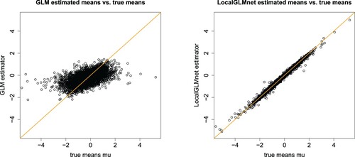13) ). This is also verified by Figure 1 (lhs) which compares the GLM estimated means $\hat{\mu }\left({\mathit{x}}_t\right)$ to the true means $\mu \left({\mathit{x}}_t\right)$ for different instances ${\mathit{x}}_t$. A perfect model would provide points on the diagonal orange line, and we see rather big differences between the GLM and the true regression function μ.

Figure 1. Estimated means $\hat{\mu }\left({\mathit{x}}_t\right)$ vs. true means $\mu \left({\mathit{x}}_t\right)$: (lhs) fitted GLM (13(13) $\mathit{x}\mapsto \mu \left(\mathit{x}\right)=\eta \left(\mathit{x}\right)={\text{β}}_0+〈\text{β},\mathit{x}〉,$(13) ) and (rhs) fitted LocalGLMnet of 5000 randomly selected out-of-sample instances ${\mathit{x}}_t$ from $\mathcal{T}$.

We could now start to improve (13(13) $\mathit{x}\mapsto \mu \left(\mathit{x}\right)=\eta \left(\mathit{x}\right)={\text{β}}_0+〈\text{β},\mathit{x}〉,$(13) ), e.g. by including a quadratic term. We refrain from doing so, but we fit the LocalGLMnet architecture (7(7) $\mathit{x}\mapsto g\left(\mu \right)=g\left(\mu \right(\mathit{x}\left)\right)={\text{β}}_0+〈\text{β}\left(\mathit{x}\right),\mathit{x}〉.$(7) ) using the identity link for g, a network of depth d = 4 having $(q_0,q_1,q_2,q_3,q_4)=(8,20,15,10,8)$ neurons, and as activation functions ${\varphi }_m$ we choose the hyperbolic tangent function for layers m = 1, 2, 3 and the linear function for m = 4. This architecture is illustrated in Listing 1 in the appendix. This LocalGLMnet is fitted using the nadam version of SGD; early stopping is tracked by using 20% of the learning data $\mathcal{L}$ as validation data $\mathcal{V}$ and the remaining 80% as training data $\mathcal{U}$, and the network calibration with the smallest MSE validation loss on $\mathcal{V}$ is selected; note that $\mathcal{L}=\mathcal{U}\cup \mathcal{V}$ is disjoint from the test data $\mathcal{T}$. This fitting approach is state-of-the-art, for more details we refer to Section 7.2.3 in Wüthrich & Merz (2021). Typically, the SGD algorithm starts in a random initialization, e.g. using the Glorot initializer. We use a special initialization in the last hidden layer ${\mathit{z}}^{\left(d\right)}$, here. Namely, we set all weights to zero ${\mathit{w}}_j^{\left(d\right)}=\mathbf{0}$, $1\le j\le q$, and the biases in this last hidden layer are initialized with the GLM parameter estimate $(w_{0,1}^{\left(d\right)},\dots ,w_{0,q}^{\left(d\right)}{)}^{\mathrm{\top }}={\widehat{\text{β}}}^{\mathrm{M}\mathrm{L}\mathrm{E}}$, see (14(14) $({\widehat{\text{β}}}_0^{\mathrm{M}\mathrm{L}\mathrm{E}},{\widehat{\text{β}}}^{\mathrm{M}\mathrm{L}\mathrm{E}})=\underset{({\text{β}}_0,\text{β})}{\arg min}\frac{1}{n}\sum _{i=1}^n{(Y_i-\mu ({\mathit{x}}_i\left)\right)}^2.$(14) ). This choice implies that we start the SGD algorithm directly in the GLM that we try to improve by learning potentially non-constant attention weights $\text{β}\left(\mathit{x}\right)$. This initialization also mitigates identifiability issue (10(10) ${\text{β}}_j\left(\mathit{x}\right)x_j=x_{j^{\prime }},$(10) ), because the LocalGLMnet has already rather pre-determined (linear) terms by this initialization.

The fitting results are given on line (d) of Table 1. The MSEs (in-sample and out-of-sample) are very close to 1 which indicates that the LocalGLMnet is able to find the true regression structure (13(13) $\mathit{x}\mapsto \mu \left(\mathit{x}\right)=\eta \left(\mathit{x}\right)={\text{β}}_0+〈\text{β},\mathit{x}〉,$(13) ). This is verified by Figure 1 (rhs) which plots the estimated means $\hat{\mu }\left({\mathit{x}}_t\right)$ against the true means $\mu \left({\mathit{x}}_t\right)$ (out-of-sample) for 5000 randomly selected instances ${\mathit{x}}_t$ from $\mathcal{T}$. The fitted LocalGLMnet estimators lie on the diagonal which says that we have good accuracy.

We are now ready to benefit from the LocalGLMnet architecture. We study the estimated regression attentions and the resulting terms in the LocalGLMnet regression function $\mathit{x}\mapsto {\widehat{\text{β}}}_j\left(\mathit{x}\right)\mathrm{a}\mathrm{n}\mathrm{d}\mathit{x}\mapsto {\widehat{\text{β}}}_j\left(\mathit{x}\right)x_j.$The interpretation to these terms has been given in Remarks 2.3. We use the code of Listing 2 to extract $\widehat{\text{β}}\left(\mathit{x}\right)$ from the fitted LocalGLMnet. These estimated regression attentions ${\widehat{\text{β}}}_j\left(\mathit{x}\right)$ are illustrated in Figure 2 by the black dots for all components $1\le j\le q=8$.

Figure 2. Regression attentions ${\widehat{\text{β}}}_j\left({\mathit{x}}_t\right)$, $1\le j\le q=8$, of 5000 randomly selected out-of-sample instances ${\mathit{x}}_t$ from $\mathcal{T}$; the y-scale is identical in all plots and on the x-scale we have $x_j$.

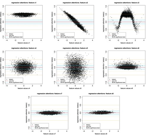
We interpret Figure 2. Regression attention ${\widehat{\text{β}}}_1\left(\mathit{x}\right)$ is concentrated around 1/2 which describes the first term in (11(11) $\mathit{x}=(x_1,\dots ,x_8{)}^{\mathrm{\top }}\in {\mathbb{R}}^8\mapsto \mu (\mathit{x})=\frac{1}{2}{x}_1-\frac{1}{4}{x}_2^2+\frac{1}{2}|x_3|\sin (2x_3)+\frac{1}{2}{x}_4{x}_5+\frac{1}{8}{x}_5^2{x}_6,$(11) ). Regression attentions ${\widehat{\text{β}}}_2\left(\mathit{x}\right),\dots ,{\widehat{\text{β}}}_6\left(\mathit{x}\right)$ are quite different from 0 (red horizontal line) which indicates that $x_2,\dots ,x_6$ are important in the description of the true regression function μ. Finally, ${\widehat{\text{β}}}_7\left(\mathit{x}\right)$ and ${\widehat{\text{β}}}_8\left(\mathit{x}\right)$ are concentrated around zero (light cyan stripe), which indicates that feature information $x_7$ and $x_8$ may not be important for our regression function; the construction of the light cyan stripe is explained in the next section on variable selection. Thus the last two variables could be dropped from the model, unless they play an important role in $\widehat{\text{β}}\left(\mathit{x}\right)$. This can be checked by just refitting the model without these variables. Figure 2 also shows that some regression attentions vary smoothly, ${\widehat{\text{β}}}_2\left(\mathit{x}\right)$ and ${\widehat{\text{β}}}_3\left(\mathit{x}\right)$, this highlights that the terms $x_2$ and $x_3$ do not exhibit interactions with other variables, in fact, ${\widehat{\text{β}}}_2\left(\mathit{x}\right)$ suggest a linear term with slope $-1/4$ which indeed is the case, see (11(11) $\mathit{x}=(x_1,\dots ,x_8{)}^{\mathrm{\top }}\in {\mathbb{R}}^8\mapsto \mu (\mathit{x})=\frac{1}{2}{x}_1-\frac{1}{4}{x}_2^2+\frac{1}{2}|x_3|\sin (2x_3)+\frac{1}{2}{x}_4{x}_5+\frac{1}{8}{x}_5^2{x}_6,$(11) ), and ${\widehat{\text{β}}}_3\left(\mathit{x}\right)$ has a sine behavior. Other attention weights ${\widehat{\text{β}}}_j\left(\mathit{x}\right)$, $4\le j\le 6$, look rather non-smooth (are dispersed). This indicates that these terms have significant interactions with other variables.

3.2. Variable selection

In the previous example, we have just said that we should drop variables $x_7$ and $x_8$ from the LocalGLMnet regression because regression attentions ${\widehat{\text{β}}}_7\left(\mathit{x}\right)$ and ${\widehat{\text{β}}}_8\left(\mathit{x}\right)$ spread around zero (are in the light cyan stripe). Obviously, these two estimators should be identically equal to zero because they do not appear in the true regression function $\mu (\cdot )$, but the noise in the data $Y_i$ is letting their estimators fluctuate around zero. This fluctuation is of comparable size for both $x_7$ (which is independent of all other variables) and $x_8$ (which is correlated with $x_2$). The main question is: how much fluctuation around zero is still acceptable for allowing to drop a variable, i.e. does not reject the null hypothesis $H_0$ of setting ${\text{β}}_7\left(\mathit{x}\right)=0$, or how much fluctuation reveals real regression structure? In GLMs, this question is answered by either computing the Wald test or the likelihood ratio test (LRT) which use asymptotic normality of MLEs, see Section 2.2.2 of Fahrmeir & Tutz (1994). Here, we cannot rely on an asymptotic theory for MLEs because early stopping implies that we do not consider the MLE. An analysis of the results also shows that the volatility in ${\widehat{\text{β}}}_7\left(\mathit{x}\right)$ is bigger than the magnitudes used in the Wald test and the LRT. For this reason, we propose an empirical way of determining the rejection region of the null hypothesis $H_0:{\text{β}}_7\left(\mathit{x}\right)=0$.

If we are given a statistical problem with features $\mathit{x}=(x_1,\dots ,x_q{)}^{\mathrm{\top }}\in {\mathbb{R}}^q$, we propose to extend these features by an additional variable $x_{q+1}$ which is completely random, independent of $\mathit{x}$ and which, of course, does not enter the true (unknown) regression function $\mu \left(\mathit{x}\right)$, but is only included in the network. This additional random component $x_{q+1}$ will quantify the magnitudes of the fluctuations in ${\widehat{\text{β}}}_{q+1}\left(\mathit{x}\right)$ of an independent component that does not enter the regression function. To successfully apply this empirical test we need to normalize all feature components $x_j$, $1\le j\le q+1$, to have zero empirical mean and unit variance, i.e. they should all live on the same scale. Note that such a normalization should already have been done for successful SGD fitting, thus, this does not impose an additional step, here. We then fit a LocalGLMnet (6(6) $\begin{array}{rl}\text{β}:{\mathbb{R}}^q& \to {\mathbb{R}}^q\\ \mathit{x}& \mapsto \text{β}\left(\mathit{x}\right)={\mathit{z}}^{(d:1)}\left(\mathit{x}\right)=({\mathit{z}}^{\left(d\right)}\circ \cdots \circ {\mathit{z}}^{\left(1\right)})\left(\mathit{x}\right).\end{array}$(6) )–(7(7) $\mathit{x}\mapsto g\left(\mu \right)=g\left(\mu \right(\mathit{x}\left)\right)={\text{β}}_0+〈\text{β}\left(\mathit{x}\right),\mathit{x}〉.$(7) ) to the learning data $\mathcal{L}$ with extended features ${\mathit{x}}^{+}=({\mathit{x}}^{\mathrm{\top }},x_{q+1}{)}^{\mathrm{\top }}\in {\mathbb{R}}^{q+1}$ which gives us the estimated regression attentions ${\widehat{\text{β}}}_1\left({\mathit{x}}_i^{+}\right),\dots ,{\widehat{\text{β}}}_{q+1}\left({\mathit{x}}_i^{+}\right)$. Using these estimated regression attentions, we receive empirical mean and standard deviation for the additional component (15) ${\overline{b}}_{q+1}=\frac{1}{n}\sum _{i=1}^n{\widehat{\text{β}}}_{q+1}\left({\mathit{x}}_i^{+}\right)\mathrm{a}\mathrm{n}\mathrm{d}{\hat{s}}_{q+1}=\sqrt{\frac{1}{n-1}\sum _{i=1}^n{\left({\widehat{\text{β}}}_{q+1}\right({\mathit{x}}_i^{+})-{\overline{b}}_{q+1})}^2}.$(15) Since this additional component $x_{q+1}$ does not enter the true regression function we expect ${\overline{b}}_{q+1}\approx 0$, and ${\hat{s}}_{q+1}$ quantifies the expected magnitude of fluctuations around zero.

The null hypothesis $H_0:{\text{β}}_j\left(\mathit{x}\right)=0$ for component j on significance level $\alpha \in (0,1/2)$ can then be rejected if the coverage ratio of the following centered interval $I_{\alpha }$ for ${\widehat{\text{β}}}_j\left({\mathit{x}}_i^{+}\right)$, $1\le i\le n$, (16) $I_{\alpha }=\left[q_{\mathcal{N}}\right(\alpha /2)\cdot {\hat{s}}_{q+1},q_{\mathcal{N}}(1-\alpha /2)\cdot {\hat{s}}_{q+1}]=\left[q_{\mathcal{N}}\right(\alpha /2)\cdot {\hat{s}}_{q+1},-q_{\mathcal{N}}(\alpha /2)\cdot {\hat{s}}_{q+1}]$(16) is substantially smaller than 1-α, where $q_{\mathcal{N}}\left(p\right)$ denotes the quantile of the standard Gaussian distribution on quantile level $p\in (0,1)$.

We come back to our Figure 2. We do not add an additional component $x_{q+1}$, but we directly use component $x_7$ to test the null hypotheses $H_0:{\text{β}}_j\left(\mathit{x}\right)=0$ for the remaining components $j\ne 7$. In our synthetic data example we have ${\overline{b}}_7=-0.0068\approx 0\mathrm{a}\mathrm{n}\mathrm{d}{\hat{s}}_7=\mathrm{0.0461.}$We choose significance level $\alpha =0.1\mathrm{\%}$ which provides us with $q_{\mathcal{N}}\left(0.05\mathrm{\%}\right)=3.2905$. The light cyan stripe in Figure 2 shows the resulting interval $I_{\alpha }$, given in (16(16) $I_{\alpha }=\left[q_{\mathcal{N}}\right(\alpha /2)\cdot {\hat{s}}_{q+1},q_{\mathcal{N}}(1-\alpha /2)\cdot {\hat{s}}_{q+1}]=\left[q_{\mathcal{N}}\right(\alpha /2)\cdot {\hat{s}}_{q+1},-q_{\mathcal{N}}(\alpha /2)\cdot {\hat{s}}_{q+1}]$(16) ), for our example. Only for $x_8$ the black dots ${\widehat{\text{β}}}_8\left({\mathit{x}}_t\right)$ are within these confidence bounds $I_{\alpha }$ which implies that we should drop this component and keep components $x_1,\dots ,x_6$ in the regression model. Note that $x_8$ and $x_2$ are correlated, and still our empirical Wald test does not reject the null hypothesis of setting ${\text{β}}_8\left(\mathit{x}\right)=0$. That is, we do the right decision, and there is no information leakage, here, through the correlated feature components. In a final step, the model with dropped components should be re-fitted and the out-of-sample loss should not substantially change, this re-fitting step verifies that the dropped components also do not play a significant role in the regression attentions ${\widehat{\text{β}}}_j\left(\mathit{x}\right)$ of the remaining feature components j, i.e. contribute by interacting with other variables.

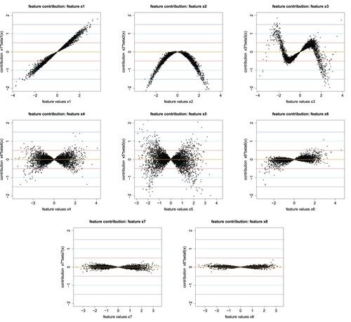
Figure 3 gives the resulting feature contributions ${\widehat{\text{β}}}_j\left({\mathit{x}}_t\right)x_{t,j}$, $1\le j\le q=8$, to the LocalGLMnet estimated regression function $\hat{\mu }\left({\mathit{x}}_t\right)$. We clearly see the linear term in $x_1$, the quadratic term in $x_2$ and the sine term in $x_3$ (first line of Figure 3), see also (11(11) $\mathit{x}=(x_1,\dots ,x_8{)}^{\mathrm{\top }}\in {\mathbb{R}}^8\mapsto \mu (\mathit{x})=\frac{1}{2}{x}_1-\frac{1}{4}{x}_2^2+\frac{1}{2}|x_3|\sin (2x_3)+\frac{1}{2}{x}_4{x}_5+\frac{1}{8}{x}_5^2{x}_6,$(11) ) for the true regression function μ. The second line of Figure 3 shows the interacting feature components $x_4$, $x_5$ and $x_6$, and the last line those that should be dropped.

Figure 3. Feature contributions ${\widehat{\text{β}}}_j\left({\mathit{x}}_t\right)x_{t,j}$, $1\le j\le q=8$, to the LocalGLMnet estimated regression function $\hat{\mu }\left({\mathit{x}}_t\right)$ of 5000 randomly selected out-of-sample instances ${\mathit{x}}_t$ from $\mathcal{T}$; the y-scale is identical in all plots and on the x-scale we have $x_j$; the horizontal lines indicate the magnitude of the feature contributions in increments of 0.5.

3.3. Interactions

In the next and final step, we explore interactions between different feature components. This is based on analyzing the gradients $\mathrm{\nabla }{\text{β}}_j\left(\mathit{x}\right)$ for $1\le j\le q$, see (9(9) $\mathrm{\nabla }{\text{β}}_j\left(\mathit{x}\right)={\left(\frac{\mathrm{\partial }}{\mathrm{\partial }{x}_1}{\text{β}}_j\right(\mathit{x}),\dots ,\frac{\mathrm{\partial }}{\mathrm{\partial }{x}_q}{\text{β}}_j(\mathit{x}\left)\right)}^{\mathrm{\top }}\in {\mathbb{R}}^q.$(9) ). The jth component of this gradient $\mathrm{\nabla }{\text{β}}_j\left(\mathit{x}\right)$ explores whether we have a linear term in $x_j$ or not. If there are no interactions of the jth component with other components, i.e. ${\text{β}}_j\left(\mathit{x}\right)x_j={\text{β}}_j\left(x_j\right)x_j$, it will exactly provide us with the right functional form of ${\text{β}}_j\left(\mathit{x}\right)$ since in that case $\mathrm{\partial }{\text{β}}_j\left(\mathit{x}\right)/\mathrm{\partial }{x}_{j^{\prime }}=0$ for all $j^{\prime }\ne j$. In relation to Figure 2 this means that the scatter plot resembles a line that does not have any lateral dilation. In Figure 2, this is the case for components $x_1,x_2,x_7,x_8$, for component $x_3$ this is not completely clear from the scatter plot, and $x_4,x_5,x_6$ show lateral extensions indicating interactions. In this latter general case, we have $\mathrm{\partial }{\text{β}}_j\left(\mathit{x}\right)/\mathrm{\partial }{x}_{j^{\prime }}\ne 0$ for some $j^{\prime }\ne j$.

We calculate the gradients $\mathrm{\nabla }{\widehat{\text{β}}}_j\left(\mathit{x}\right)$, $1\le j\le q$, of the fitted model. These can be obtained by the R code of Listing 3. This provides us for fixed j with vectors $\mathrm{\nabla }{\widehat{\text{β}}}_j\left({\mathit{x}}_i\right)$ for all instances $i=1,\dots ,n$. To analyze these gradients, we fit a spline to these observations by regressing (17) ${\mathrm{\partial }}_{x_k}{\widehat{\text{β}}}_j\left({\mathit{x}}_i\right)=\frac{\mathrm{\partial }}{\mathrm{\partial }{x}_k}{\widehat{\text{β}}}_j\left({\mathit{x}}_i\right)\sim x_{i,j}.$(17) This studies the derivative of regression attention ${\widehat{\text{β}}}_j\left(\mathit{x}\right)$ w.r.t. $x_k$ as a function of the corresponding feature component $x_j$ that is considered in the feature contribution ${\text{β}}_j\left(\mathit{x}\right)x_j$, see (7(7) $\mathit{x}\mapsto g\left(\mu \right)=g\left(\mu \right(\mathit{x}\left)\right)={\text{β}}_0+〈\text{β}\left(\mathit{x}\right),\mathit{x}〉.$(7) ). The code for these spline fits is also provided in Listing 3 on lines 12–15, and it gives us the results illustrated in Figure 4.

Figure 4. Spline fits to the sensitivities ${\mathrm{\partial }}_{x_k}{\widehat{\text{β}}}_j\left({\mathit{x}}_i\right)$, $1\le j,k\le 6$, over all instances $i=1,\dots ,n$.

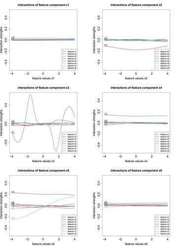
Figure 4 studies the spline regressions (17(17) ${\mathrm{\partial }}_{x_k}{\widehat{\text{β}}}_j\left({\mathit{x}}_i\right)=\frac{\mathrm{\partial }}{\mathrm{\partial }{x}_k}{\widehat{\text{β}}}_j\left({\mathit{x}}_i\right)\sim x_{i,j}.$(17) ) only of the significant components $x_1,\dots ,x_6$ that enter regression function μ, see (11(11) $\mathit{x}=(x_1,\dots ,x_8{)}^{\mathrm{\top }}\in {\mathbb{R}}^8\mapsto \mu (\mathit{x})=\frac{1}{2}{x}_1-\frac{1}{4}{x}_2^2+\frac{1}{2}|x_3|\sin (2x_3)+\frac{1}{2}{x}_4{x}_5+\frac{1}{8}{x}_5^2{x}_6,$(11) ). We interpret these plots.

• Plot $x_1$ shows that all gradients are roughly zero, which means that ${\text{β}}_1\left(\mathit{x}\right)=\mathrm{c}\mathrm{o}\mathrm{n}\mathrm{s}\mathrm{t}$, which, indeed, is the case in the true regression function μ.

• Plots $x_2$ and $x_3$ show one term that is significantly different from 0. For the $x_2$ plot it is ${\mathrm{\partial }}_{x_2}{\widehat{\text{β}}}_2\left(\mathit{x}\right)$, and for the $x_3$ plot it is ${\mathrm{\partial }}_{x_3}{\widehat{\text{β}}}_3\left(\mathit{x}\right)$. This says that these two terms do not have any interactions with other variables, and that the right functional form is not the linear one, but ${\widehat{\text{β}}}_j\left(\mathit{x}\right)x_j={\widehat{\text{β}}}_j\left(x_j\right)x_j$ is non-linear for j = 2, 3. In fact, we have ${\mathrm{\partial }}_{x_2}{\widehat{\text{β}}}_2\left(\mathit{x}\right)\approx \mathrm{c}\mathrm{o}\mathrm{n}\mathrm{s}\mathrm{t}$ which says that we have a quadratic term in $x_2$, and ${\mathrm{\partial }}_{x_3}{\widehat{\text{β}}}_3\left(\mathit{x}\right)$ shows a sine like behavior.

• Plot $x_4$ shows a linear interaction with $x_5$ because ${\mathrm{\partial }}_{x_5}{\widehat{\text{β}}}_4\left(\mathit{x}\right)\approx \mathrm{c}\mathrm{o}\mathrm{n}\mathrm{s}\mathrm{t}$.

• Plot $x_5$ shows a linear interaction with $x_4$ because ${\mathrm{\partial }}_{x_4}{\widehat{\text{β}}}_5\left(\mathit{x}\right)\approx \mathrm{c}\mathrm{o}\mathrm{n}\mathrm{s}\mathrm{t}$, and it shows an interaction with $x_6$.

• Plot $x_6$ does not show any significant terms, as they have already been captured by the previous plots. Note that this comes from the fact that terms $x_5^2{x}_6/8$ do not lead to an identifiable decomposition, but this can be allocated either to $x_5$ or to $x_6$, or could even be split among the two.

We give concluding remarks on this synthetic data example. In general, interpretation is simpler if we have ${\text{β}}_j\left(\mathit{x}\right)={\text{β}}_j\left(x_j\right)$, i.e. if the components do not have interactions, because this results in rather smooth curves in Figure 3. This may be achieved by pre-processing features, e.g. we may consider the body mass index, instead of using the weight and the height of a person (if there is corresponding interaction in the regression function). Additionally, we can also use the functional forms found by the LocalGLMnet, e.g. we have seen that component $x_2$ enters the regression function as a quadratic term, and we could fit another LocalGLMnet using feature component $x_2^2$, instead. This may provide even clearer and better explanations.

3.4. Real data example

As a second example we consider a real data example. In this real data example, we also discuss how categorical feature components should be pre-processed for our LocalGLMnet approach. We consider the French motor third party liability (MTPL) claims frequency data FreMTPL2freq which is available through the R package CASdatasets of Dutang & Charpentier (2018). This dataset has been used within the actuarial literature as a standard benchmark for the application of machine learning methods to the problem of non-life pricing and is described in Appendix A of Wüthrich & Merz (2021) and in the tutorials of Noll et al. (2018) and Lorentzen & Mayer (2020). Some other works focusing on this dataset are Kuo (2019), Richman (2020), Richman & Wüthrich (2020), and Delong & Kozak (2021), among others. We apply the data cleaning of Listing B.1 of Wüthrich & Merz (2021) to this data. After data cleaning, we have observations $(Y_i,v_i,{\mathit{x}}_i{)}_i$ with claim counts $Y_i\in {\mathbb{N}}_0$, time exposures $v_i\in (0,1]$ and feature information ${\mathit{x}}_i$. We have six continuous feature components (called ‘Area Code’, ‘Bonus-Malus Level’, ‘Density’, ‘Driver's Age’, ‘Vehicle Age’, ‘Vehicle Power’), 1 binary component (called ‘Vehicle Gas’) and two categorical components with more than two levels (called ‘Vehicle Brand’ and ‘Region’). We pre-process these components as follows: we center and normalize to unit variance the six continuous and the binary components. We apply one-hot encoding to the two categorical variables, we emphasize that we do not use dummy coding as it is usually done in GLMs. Below, in Section 3.6, we are going to motivate this one-hot encoding choice (which does not lead to full rank design matrices); for one-hot encoding vs. dummy coding we refer to formulas (5.21) and (7.29) in Wüthrich & Merz (2021).

As a control variable, we add two random feature components that are i.i.d., centered and with unit variance, the first one having a uniform distribution and the second one having a standard normal distribution, we call these two additional feature components ‘RandU’ and ‘RandN’. We consider two additional independent components to understand whether the distributional choice influences the results of hypothesis testing using the empirical interval $I_{\alpha }$, see (16(16) $I_{\alpha }=\left[q_{\mathcal{N}}\right(\alpha /2)\cdot {\hat{s}}_{q+1},q_{\mathcal{N}}(1-\alpha /2)\cdot {\hat{s}}_{q+1}]=\left[q_{\mathcal{N}}\right(\alpha /2)\cdot {\hat{s}}_{q+1},-q_{\mathcal{N}}(\alpha /2)\cdot {\hat{s}}_{q+1}]$(16) ). Altogether (and using one-hot encoding) we receive q = 42 dimensional tabular feature variables ${\mathit{x}}_i\in {\mathbb{R}}^q$; this includes the two additional components RandU and RandN.

We fit a Poisson network regression model to this French MTPL data. Note that the Poisson distribution belongs to the EDF with cumulant function $\kappa \left(\theta \right)=\exp \left\{\theta \right\}$ on the effective domain $\mathbf{\Theta }=\mathbb{R}$. The canonical link is given by the log-link, this motivates link choice $g(\cdot )=\log (\cdot )$. We then start by fitting a plain-vanilla FFN network (5(5) $\mathit{x}\mapsto g\left(\mu \right)=g\left(\mu \right(\mathit{x}\left)\right)={\text{β}}_0+〈\text{β},{\mathit{z}}^{(d:1)}\left(\mathit{x}\right)〉,$(5) ) to this data. This FFN network will give us the benchmark in terms of predictive power. We choose a network of depth d = 3 having $(q_1,q_2,q_3)=(20,15,10)$ FFN neurons; the R code for this FFN architecture is given in Listing 7.1 of Wüthrich & Merz (2021), but we replace input dimension 40 by 42 on line 3 of that listing to account for the two additional feature components ‘RandU’ and ‘RandN’. To do a proper out-of-sample generalization analysis we partition the data randomly into a learning data set $\mathcal{L}$ and a test data set $\mathcal{T}$. The learning data $\mathcal{L}$ contains n = 610, 206 instances and the test data set $\mathcal{T}$ contains 67, 801 instances; we use exactly the same split as in Table 5.2 of Wüthrich & Merz (2021). The learning data $\mathcal{L}$ will be used to learn the network parameters and the test data $\mathcal{T}$ is used to perform an out-of-sample generalization analysis. As loss function for parameter fitting and generalization analysis we choose the Poisson deviance loss, which is a distribution adapted and strictly consistent loss function for the mean within the Poisson model, for details we refer to Section 4.1.3 in Wüthrich & Merz (2021).

We fit this FFN network using the nadam version of SGD on batches of size 5000 over 100 epochs, and we retrieve the network calibration that provides the smallest validation loss on a training-validation partition $\mathcal{U}$ and $\mathcal{V}$ of the learning data $\mathcal{L}$. The results are presented on line (b) of Table 2. The FFN network provides clearly better results than the null model only using a bias ${\text{β}}_0$. This justifies regression modeling, here.

Table 2. In-sample and out-of-sample losses on the real MTPL data example.

	Poisson deviance losses in ${10}^{-2}$
	In-sample on $\mathcal{L}$	Out-of-sample on $\mathcal{T}$
(a) null model (bias ${\text{β}}_0$ only)	25.213	25.445
(b) FFN network	23.764	23.873
(c) LocalGLMnet	23.728	23.945
(d) reduced LocalGLMnet	23.714	23.912
(e) Poisson GLM3	24.084	24.102
(f) Categorical Embedding network	23.690	23.824
(g) Nagging network	23.691	23.783

Next we fit the LocalGLMnet architecture using exactly the same set up as in the FFN network, but having a depth of d = 4 with numbers of neurons $(q_0,q_1,q_2,q_3,q_4)=(42,20,15,10,42)$. The results on line (c) of Table 2 show that we sacrifice a bit of predictive power (out-of-sample) for receiving our interpretable network architecture. Moreover, we complement the table with results of Wüthrich & Merz (2021) fitting several other models to the same data, namely, a GLM on line (e), an FFN which encodes the categorical features using embedding layers on line (f), and an ensemble of networks using the nagging predictor on line (g). Compared to the GLM, which is currently the industry standard for non-life claim frequency prediction, the LocalGLMnet model performs significantly better (out-of-sample). The FFN with embedding layers and the ensemble of networks outperform both the LocalGLMnet and the simple FFN on line (b). Thus for the LocalGLMnet we sacrifice a little bit of predictive performance for having an explainable predictive model. On the other hand, we can perform variable selection with the LocalGLMnet, and if the ultimate goal is predictive performance we can still fit another network architecture to the LocalGLMnet-selected variables.

We now analyze the resulting estimated regression attentions ${\widehat{\text{β}}}_j\left(\mathit{x}\right)$. We start by studying the regression attentions ${\widehat{\text{β}}}_j\left(\mathit{x}\right)$ of the continuous and binary feature components Area Code, Bonus-Malus Level, Density, Driver's Age, Vehicle Age, Vehicle Gas, Vehicle Power, RandU and RandN. First, we calculate the empirical standard deviations ${\hat{s}}_j$ that we receive from RandU and RandN, see (15(15) ${\overline{b}}_{q+1}=\frac{1}{n}\sum _{i=1}^n{\widehat{\text{β}}}_{q+1}\left({\mathit{x}}_i^{+}\right)\mathrm{a}\mathrm{n}\mathrm{d}{\hat{s}}_{q+1}=\sqrt{\frac{1}{n-1}\sum _{i=1}^n{\left({\widehat{\text{β}}}_{q+1}\right({\mathit{x}}_i^{+})-{\overline{b}}_{q+1})}^2}.$(15) ), ${\hat{s}}_{\mathrm{R}\mathrm{a}\mathrm{n}\mathrm{d}\mathrm{U}}=0.052\mathrm{a}\mathrm{n}\mathrm{d}{\hat{s}}_{\mathrm{R}\mathrm{a}\mathrm{n}\mathrm{d}\mathrm{N}}=\mathrm{0.048.}$Thus these standard deviation estimates are rather similar, and in this case the specific distributional choice of the control variable $x_{q+1}$ does not influence the results. We discuss further these distributional choices and alternative choices together with an analysis of impact of sampling error in Appendix 2. We calculate interval $I_{\alpha }$ for significance level $\alpha =0.1\mathrm{\%}$, see (16(16) $I_{\alpha }=\left[q_{\mathcal{N}}\right(\alpha /2)\cdot {\hat{s}}_{q+1},q_{\mathcal{N}}(1-\alpha /2)\cdot {\hat{s}}_{q+1}]=\left[q_{\mathcal{N}}\right(\alpha /2)\cdot {\hat{s}}_{q+1},-q_{\mathcal{N}}(\alpha /2)\cdot {\hat{s}}_{q+1}]$(16) ). The resulting interval $I_{\alpha }$ is illustrated by the light cyan stripes in Figure 5. We observe that for the variables Bonus–Malus Level, Density, Driver's Age, Vehicle Age and Vehicle Gas we clearly reject the null hypothesis $H_0:{\text{β}}_j\left(\mathit{x}\right)=0$ on the chosen significance level $\alpha =0.1\mathrm{\%}$, and Area Code and Vehicle Power need further analysis. For these two variables, $I_{\alpha }$ provides a coverage ratio of 97.1% and 98.1%, thus, strictly speaking these numbers are below $1-\alpha =99.9\mathrm{\%}$ and we should keep these variables in the model. 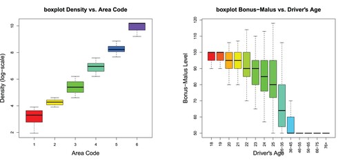Nevertheless, since there is some sampling error in deriving ${\hat{s}}_{\mathrm{R}\mathrm{a}\mathrm{n}\mathrm{d}\mathrm{U}}$ and ${\hat{s}}_{\mathrm{R}\mathrm{a}\mathrm{n}\mathrm{d}\mathrm{N}}$, e.g. the appendix shows that different samples for these variables could produce slightly wider intervals, we further analyze these two variables. From the empirical analysis in Noll et al. (2018) we know that Area Code and Density are highly correlated. Figure 6 (lhs) shows the boxplot of Density vs. Area Code, and this plot highlights that Density almost fully explains Area Code. Therefore, it is sufficient to include the Density variable and we drop Area Code.

Figure 5. Attention weights ${\text{β}}_j\left({\mathit{x}}_t\right)$ of the continuous and binary feature components Area Code, Bonus-Malus Level, Density, Driver's Age, Vehicle Age, Vehicle Gas, Vehicle Power, RandU and RandN for 5000 randomly selected instances ${\mathit{x}}_t$ of $\mathcal{T}$; the light cyan stripe shows the confidence area $I_{\alpha }$ on significance level $\alpha =0.1\mathrm{\%}$.

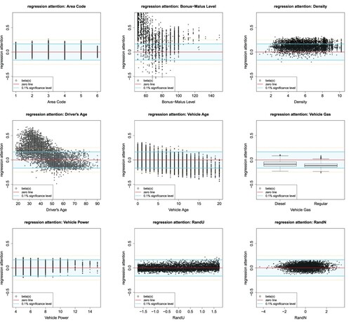
Figure 6. (lhs) Boxplots of Density vs. Area Code and (rhs) Bonus-Malus vs. Driver's Age.

Thus, we drop the variables Area Code and VehPower, and we also drop the control variables RandU and RandN, because these are no longer needed. This gives us a reduced input dimension of $q_0=q=38$, and we run the same LocalGLMnet SGD fitting again. Line (d) of Table 2 gives the in-sample and out-of-sample results of this reduced LocalGLMnet model. We observe a small out-of-sample improvement compared to line (c) which confirms that we can drop Area Code and VehPower without losing predictive performance. In fact, the small improvement indicates that a smaller model less likely over-fits, and we can consider more SGD steps before over-fitting, i.e. we receive a later early stopping point.

Having performed variable selection and dropping unimportant variables, another approach would be to then fit a different model to the reduced set of features, for example an FFN, which would provide better out-of-sample performance than the LocalGLMnet. This approach is advisable if the emphasis is on predictive performance instead of interpretability.

Figure 7 shows the feature contributions ${\widehat{\text{β}}}_j\left({\mathit{x}}_t\right)x_{j,t}$ of the selected continuous and binary feature components Bonus–Malus Level, Density, Driver's Age, Vehicle Age and Vehicle Gas of 5000 randomly selected instances ${\mathit{x}}_t$, and the magenta line shows a spline fit to these feature contributions; the y-scale is the same in all plots. We observe that all these components contribute substantially to the regression function, the Bonus–Malus variable being the most important one, and Vehicle Gas being the least important one. Bonus–Malus and Density have in average an increasing trend, and Vehicle Age has in average a decreasing trend, Density being close to a linear function, and the remaining continuous variables are clearly non-linear. The explanation of Driver's Age is more difficult as can be seen from the spline fit (magenta color). Figure 6 (rhs) shows the boxplot of Bonus–Malus Level vs. Driver's Age. We observe that new (young) drivers enter the bonus-malus system at 100, and every year of driving without an accident decreases the bonus-malus level. Therefore, the lowest bonus-malus level can only be reached after multiple years of accident-free driving. This can be seen from Figure 6 (rhs), and it implies that the Bonus–Malus Level and the Driver's Age variables interact. We are going to verify this by studying the gradients $\mathrm{\nabla }{\widehat{\text{β}}}_j\left(\mathit{x}\right)$ of the regression attributions. The smoothed feature contributions of Figure 7 are compared in Appendix 2 to PDPs produced using an FFN fit to the same reduced set of variables. The comparison shows that the smoothed feature contributions are generally similar to PDPs, but differ for values of the variables where there are not many observations (note that PDPs do not consider dependence within feature vectors appropriately).

Figure 7. Feature contributions ${\widehat{\text{β}}}_j\left({\mathit{x}}_t\right)x_{j,t}$ of the continuous and binary feature components Bonus–Malus Level, Density, Driver's Age, Vehicle Age and Vehicle Gas of 5000 randomly selected instances ${\mathit{x}}_t$ of $\mathcal{T}$; the y-scale is the same in all plots and the magenta color gives a spline fit to the feature contributions.

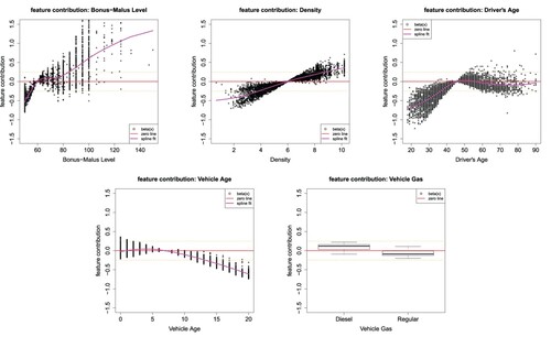
Figure 8 shows the spline fits to the gradients ${\mathrm{\partial }}_{x_k}{\widehat{\text{β}}}_j\left(\mathit{x}\right)$ of the continuous variables Bonus–Malus Level, Density, Driver's Age and Vehicle Age. First, we observe that Bonus–Malus Level and Driver's Age have substantial non-linear terms ${\mathrm{\partial }}_{x_j}{\widehat{\text{β}}}_j\left(\mathit{x}\right)x_j$, Vehicle Age shows some non-linearity and Density seems to be pretty linear since ${\mathrm{\partial }}_{x_j}{\widehat{\text{β}}}_j\left(\mathit{x}\right)x_j\approx 0$. This verifies the findings of Figure 7 of the magenta spline fits.

Figure 8. Spline fits to the gradients ${\mathrm{\partial }}_{x_k}{\widehat{\text{β}}}_j\left({\mathit{x}}_i\right)$ of the continuous variables Bonus–Malus Level, Density, Driver's Age and Vehicle Age over all instances $i=1,\dots ,n$.

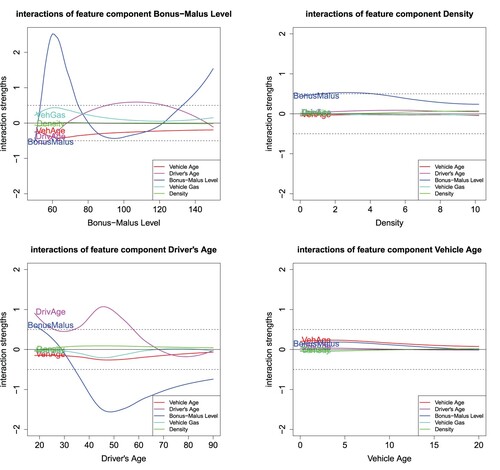
Next we focus on interactions which requires the study of ${\mathrm{\partial }}_{x_k}{\widehat{\text{β}}}_j\left(\mathit{x}\right)$ for $k\ne j$ in Figure 8. The most significant interactions can clearly be observed between Bonus–Malus Level and Driver's Age, but also between the Bonus–Malus Level and Density we encounter an interaction term saying that a higher Bonus–Malus Level at a lower Density leads to a higher prediction, which intuitively makes sense as in less densely populated areas we expect less claims. For Vehicle Age, we do not find substantial interactions, it only weakly interacts with Bonus–Malus Level and Driver's Age by entering the corresponding regression attributions ${\widehat{\text{β}}}_j\left(\mathit{x}\right)$ of these two feature components.

There remains the discussion of the categorical feature components Vehicle Brand and Region. This is going to be done in Section 3.6.

Remark 3.1

Networks fitted with early stopping in SGD do not fulfill the so-called balance property and, henceforth, may have a bias. Since we work under the canonical link choice, here, we can apply the bias regularization method proposed in Wüthrich (2020). For this we define the learned features ${\hat{z}}_{i,j}={\widehat{\text{β}}}_j\left({\mathit{x}}_i\right)x_{i,j}$, $1\le j\le q$, that is, for each instance $1\le i\le n$ we have a new learned feature ${\hat{\mathit{z}}}_i=({\hat{z}}_{i,1},\dots ,{\hat{z}}_{i,q}{)}^{\mathrm{\top }}\in {\mathbb{R}}^q$. These learned features can then be used in a classical GLM, see (2(2) $\mathit{x}\mapsto g\left(\mu \right)=g\left(\mu \right(\mathit{x}\left)\right)={\text{β}}_0+〈\text{β},\mathit{x}〉={\text{β}}_0+\sum _{j=1}^q{\text{β}}_j{x}_j,$(2) ), ${\hat{\mathit{z}}}_i\mapsto g\left(\mu \right)={\alpha }_0+〈\mathit{\alpha },{\hat{\mathit{z}}}_i〉={\alpha }_0+\sum _{j=1}^q{\alpha }_j{\hat{z}}_{i,j},$with regression parameter $({\alpha }_0,\mathit{\alpha })\in {\mathbb{R}}^{q+1}$. Since an MLE estimated GLM under canonical link choice satisfies the balance property, so will the LocalGLMnet ${\mathit{x}}_i\mapsto g\left(\mu \right)={\hat{\alpha }}_0^{\mathrm{M}\mathrm{L}\mathrm{E}}+\sum _{j=1}^q{\hat{\alpha }}_j^{\mathrm{M}\mathrm{L}\mathrm{E}}{\widehat{\text{β}}}_j\left({\mathit{x}}_i\right)x_{i,j}.$That is, we just slightly rescale the regression attentions to receive the balance property. For more on this topic, we refer to Section 7.4.2 in Wüthrich & Merz (2021).

3.5. Variable importance

The estimated regression attentions ${\widehat{\text{β}}}_j\left(\mathit{x}\right)$, $1\le j\le q$, allow us to quantify variable importance. A simple measure of variable importance can be defined by ${\mathrm{V}\mathrm{I}}_j=\frac{1}{n}\sum _{i=1}^n\left|{\widehat{\text{β}}}_j\right({\mathit{x}}_i\left)\right|,$for $1\le j\le q$ and where we aggregate over all instances $1\le i\le n$. Typically, the bigger these values ${\mathrm{V}\mathrm{I}}_j$ the more component $x_j$ influences the regression function. Note that all feature components $x_j$ have been centered and normalized to unit variance, i.e. 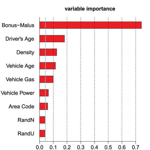they live on the same scale, otherwise such a comparison of ${\mathrm{V}\mathrm{I}}_j$ across different j would not make sense. Figure 9 gives the variable importance results, which emphasizes that Area Code and Vehicle Power are the least important variables which, in fact, have been dropped in a second step above.

Figure 9. Variable importance ${\mathrm{V}\mathrm{I}}_j$, $1\le j\le q$.

3.6. Categorical feature components

In this section, we discuss how categorical feature components can be considered. Note that at the beginning of Section 3.4, we have emphasized that we use one-hot encoding and not dummy coding for categorical variables. The reason for this choice can be seen in Figure 7. Namely, if the feature value is $x_j=0$, then the corresponding feature contribution gives ${\text{β}}_j\left(\mathit{x}\right)x_j=0$. This provides the calibration of the regression model, i.e. it gives the reference level which is determined by the bias ${\text{β}}_0\in \mathbb{R}$. Since in GLMs we do not allow the components to interact in the linear predictor $\eta \left(\mathit{x}\right)$, all instances that have the same level $x_j$ receive the same contribution ${\text{β}}_j{x}_j$, see (2(2) $\mathit{x}\mapsto g\left(\mu \right)=g\left(\mu \right(\mathit{x}\left)\right)={\text{β}}_0+〈\text{β},\mathit{x}〉={\text{β}}_0+\sum _{j=1}^q{\text{β}}_j{x}_j,$(2) ). In the LocalGLMnet, we allow the same level $x_j$ to have different contributions ${\text{β}}_j\left(\mathit{x}\right)x_j$ through interactions in the regression attention $\text{β}\left(\mathit{x}\right)$. If we want to carry this forward to categorical feature components it requires that these components receive an encoding that is not identically equal to zero. This is the case for one-hot encoding, but not for dummy coding where the reference level is just identical to the bias ${\text{β}}_0$. For this reason, we recommend to use one-hot encoding for the LocalGLMnet.

Figure 10 shows the feature contributions ${\widehat{\text{β}}}_j\left(\mathit{x}\right)$ of the categorical feature components, note that each box corresponds to one level of the chosen categorical variable. First, different medians between the boxes indicate different parameter sizes ${\widehat{\text{β}}}_j\left(\mathit{x}\right)$ for different levels j; note that in one-hot encoding j describes the different levels of the categorical variable. Second, the larger the box the more interaction this level has with other feature components, because ${\widehat{\text{β}}}_j\left({\mathit{x}}_i\right)$ is more volatile over different instances i.

Figure 10. Boxplot of the feature contributions ${\widehat{\text{β}}}_j\left(\mathit{x}\right)$ of the categorical feature components Vehicle Brand and French Regions; the y-scale is the same as in Figure 7.

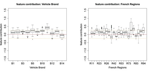
From Figure 10, we observe that Vehicle Brands B11 and B14 are the two most extreme Vehicle Brands w.r.t. claims frequency, B11 having the highest expected frequency and B14 the lowest. From the French Regions R74 (Limousin) and R82 (Rhône-Alpes) seem outstanding having a higher frequency than elsewhere. This finishes our example.

In fact, Figure 10 provides contextualized embeddings for the different levels of the categorical features. Attention-based embedding models exactly try to do such a contextualized embedding, we refer to Kuo & Richman (2021) in an actuarial context and to Huang et al. (2020) for general tabular data.

We could add the learned categorical regression attentions ${\widehat{\text{β}}}_j\left(\mathit{x}\right)$ to the variable importance plot of Figure 9. This requires some care. First, if categorical variables have many levels, then showing individual levels will not result in clear plots. Second, one-hot encoding is not normalized and centered to unit variance, thus, these one-hot encoded variables live on a different scale compared to the standardized ones, and a direct comparison is not sensible.

4. Conclusion

We have introduced the LocalGLMnet which is inspired by classical GLMs. Making the regression parameters of a generalized linear model feature dependent allows us to receive a flexible regression model that shares representation learning and the predictive performance of classical fully-connected feed-forward neural networks, and at the same time it remains interpretable. This appealing structure allows us to perform variable selection, it allows us to study variable importance and it also allows us to determine interactions. Thus it provides us with a fully transparent network model that brings out the internal structure of the data. To the best of our knowledge, this is rather unique in network regression modeling, since our proposal does not share the shortcomings of similar proposals like computational burden or a loss of predictive power.

Above we have mentioned possible extensions, e.g. LocalGLM layers can be composed to receive deeper interpretable networks, and the LocalGLMnet can serve as a surrogate model to shed more light into many other deep learning models. A different method of utilizing the LocalGLMnet would be to iteratively fit the model and then use the smoothed feature contribution and interaction plots (i.e. those shown in Figures 7 and 8) to aid the fitting of a GLM by adding new variables corresponding to these plots to the GLM. Once these are added, the LocalGLMnet could be refit to the expanded variables and the process is repeated. Another extension would be a method of constraining the regression attention coefficients to produce monotone effects which would potentially be useful in practice. However, this would require substantial modifications to the LocalGLMnet fitting process, so we leave this modification for monotonic effects (which applies equally to more general neural networks, such as FFNs) for further research. Whereas our architecture is most suitable for tabular input data, the question about optimal consideration of non-tabular data or of categorical variables with many levels is one point that should also be further explored.

Acknowledgments

We thank Christopher Blier-Wong, Friedrich Loser, Andreas Tsanakas and the two anonymous reviewers for providing very useful remarks to improve earlier versions of this manuscript.

Disclosure statement

No potential conflict of interest was reported by the author(s).

Appendices

R code

Further analysis of the real data example

Here we explore further the empirical variable selection method demonstrated on the real data example in Section 3.4, and compare the average feature contributions within the LocalGLMnet to another popular model interpretability technique, the partial dependence plot (PDP) of Friedman (2001).

B.1. Variability of variable selection method

To determine the potential variability in variable selection induced by the sampling and fitting error of the ‘RandU’ and ‘RandN’ variables, the model fitting described in Section 3.4 was repeated 100 times using exactly the same data splits and random seed for the model training, and varying only these variables by drawing new samples from these same distributions. Moreover, in a different set of 100 runs, we also replaced these variables with permuted copies of the Bonus-Malus and Vehicle Age variables. The average value of the standard deviations of the regression attentions relating to each of these variables (i.e. the average value of $\hat{s}$) that is used to estimate the confidence intervals (16(16) $I_{\alpha }=\left[q_{\mathcal{N}}\right(\alpha /2)\cdot {\hat{s}}_{q+1},q_{\mathcal{N}}(1-\alpha /2)\cdot {\hat{s}}_{q+1}]=\left[q_{\mathcal{N}}\right(\alpha /2)\cdot {\hat{s}}_{q+1},-q_{\mathcal{N}}(\alpha /2)\cdot {\hat{s}}_{q+1}]$(16) ) and the standard deviation of these are shown in Table B1. Over 100 runs, the average magnitude of $\hat{s}$ varies somewhat depending on the distributional assumption underlying the control variables and, on the other hand, the standard deviations of these are roughly constant, showing little dependence on the distributional assumptions. Since there is some sampling variability in deriving the confidence bands (16(16) $I_{\alpha }=\left[q_{\mathcal{N}}\right(\alpha /2)\cdot {\hat{s}}_{q+1},q_{\mathcal{N}}(1-\alpha /2)\cdot {\hat{s}}_{q+1}]=\left[q_{\mathcal{N}}\right(\alpha /2)\cdot {\hat{s}}_{q+1},-q_{\mathcal{N}}(\alpha /2)\cdot {\hat{s}}_{q+1}]$(16) ), as it is usually the case in statistics on finite samples, these confidence bands should be treated as indicative of the ‘true’ values, and when performing variable selection, those variables that produce regression attention values that are close in magnitude to the confidence bands should be investigated further, as is done in Section 3.4. On the other hand, adding more variables to the LocalGLMnet, for example, several permuted variables as well as randomly sampled variables, would likely increase the potential for over fitting, thus, we prefer to rely on ‘RandU’ and ‘RandN’ in the real data example.

Table B1. Sample averages and standard deviations of $\hat{s}$ over 100 different training runs.

	RandU	RandN	permute	permute
			Bonus-Malus	Vehicle Age
Sample average of $\hat{s}$	0.047	0.043	0.051	0.042
Sample standard deviation of $\hat{s}$	0.010	0.009	0.009	0.009

B.2. Comparison to partial dependence plots

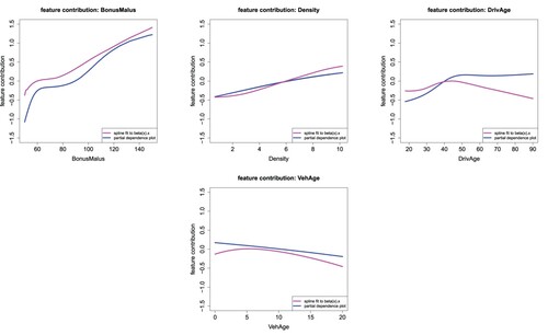
Figure 7 shows the feature contributions of each variable to the LocalGLMnet and smoothed values of the feature contributions estimated using a local spline fit. In this section, we consider whether these smoothed values can be compared to results of estimating PDPs on the reduced dataset. To make this comparison, we fit an FFN to the reduced dataset (i.e. excluding Area Code and VehPower), and then calculate PDPs for 5,000 randomly selected instances ${\mathit{x}}_t$ of $\mathcal{T}$. These are compared to the smoothed feature contributions of the remaining continuous variables in Figure B11. The PDPs generally follow a similar shape to the smoothed feature contributions for the Bonus-Malus, Density and Vehicle Age variables, but the shape is quite different for the Driver Age variable. Moreover, the magnitudes of the values of the PDPs are roughly similar to those of the smoothed feature contributions. The most significant departures of the PDPs from the smoothed feature contributions seem to occur at values of the variables with the least data (the oldest drivers and those drivers with the lowest bonus-malus scores). Whereas PDPs suffer from the well-known deficiency of assuming independence between variables, potentially leading to unlikely combinations of variables, the smoothed feature contributions show the average effects of each variable within the LocalGLMnet, likely leading to more robust and reasonable estimates of feature importance at these values of the variables, i.e. at the oldest driver ages, and lowest levels of bonus-malus, we should attribute greater credibility to the smoothed feature contributions than the PDPs. Furthermore, PDPs require significantly more computation than the smoothed feature contributions which are available directly from the LocalGLMnet.

Figure B11. Spline fit to the feature contributions ${\widehat{\text{β}}}_j\left({\mathit{x}}_t\right)x_{j,t}$ and PDPs of the continuous variables Bonus-Malus Level, Density, Driver's Age and Vehicle Age of 5,000 randomly selected instances ${\mathit{x}}_t$ of $\mathcal{T}$; the y-scale is the same in all plots.

References

- Agarwal R., Frosst N., Zhang X., Caruana R. & Hinton G. E. (2020). Neural additive models: interpretable machine learning with neural nets. arXiv:2004.13912v1.
- Ahn J., Lu Y., Oh R., Park K. & Zhu D. (2021). Neural credibility [conference presentation]. In Virtual 24th International Congress on Insurance: Mathematics and Economics, July 5–10. Urbana-Champaign, USA: University of Illinois.
- Apley D. W. & Zhu J. (2020). Visualizing the effects of predictor variables in black box supervised learning models. Journal of the Royal Statistical Society: Series B 82(4), 1059–1086.
- Arik S. Ö & Pfister T. (2019). TabNet: attentive interpretable tabular learning. arXiv:1908.07442v5.
- Bahdanau D., Cho K. & Bengio Y. (2014). Neural machine translation by jointly learning to align and translate. arXiv:1409.0473.
- Barndorff-Nielsen O. (2014). Information and exponential families: in statistical theory. Chichester, West Sussex, UK: John Wiley & Sons.
- Chen C., Li O., Tao C., Barnett A., Su J. & Rudin C. (2019). This looks like that: deep learning for interpretable image recognition. Advances in Neural Information Processing Systems 32, Vancouver, Canada.
- Delong Ł. & Kozak A. (2021). The use of autoencoders for training neural networks with mixed categorical and numerical features. SSRN Manuscript ID 3952470.
- Dutang C. & Charpentier A. (2018). CASdatasets R Package Vignette. Reference Manual. Version 1.0-8, packaged 2018-05-20.
- Fahrmeir L. & Tutz G. (1994). Multivariate statistical modelling based on generalized linear models. New York, USA: Springer.
- Friedman J. H. (2001). Greedy function approximation: a gradient boosting machine. Annals of Statistics29(5), 1189–1232.
- Goodfellow I., Bengio Y. & Courville A. (2016). Deep learning. MIT Press.
- Ha D., Dai A. & Le Q. (2016). Hypernetworks. arXiv:1609.09106.
- He K., Zhang X., Ren S. & Sun J. (2016). Deep residual learning for image recognition. In 2016 IEEE Conference on Computer Vision and Pattern Recognition, Vol. 1, P. 770–778. Las Vegas, USA.
- Huang X., Khetan A., Cvitkovic M. & Karnin Z. (2020). TabTransformer: tabular data modeling using contextual embeddings. arXiv:2012.00678.
- Jørgensen B. (1997). The theory of dispersion models. London, UK: Chapman & Hall.
- Kuo K. (2019). Generative synthesis of insurance datasets. arXiv:1912.02423v2.
- Kuo K. & Richman R. (2021). Embeddings and attention in predictive modeling. arXiv:2104.03545v1.
- Kursa M. & Rudnicki W. (2010). Feature selection with the Boruta package. Journal of Statistical Software 36, 1–13.
- Lemhadri I., Ruan F., Abraham L. & Tibshirani R. (2021). LassoNet: a neural network with feature sparsity. Journal of Machine Learning Research 22, 1–29.
- Lorentzen C. & Mayer M. (2020). Peeking into the black box: an actuarial case study for interpretable machine learning. SSRN Manuscript ID 3595944. Version May 7, 2020.
- Lundberg S. M. & Lee S.-I. (2017). A unified approach to interpreting model predictions. In Advances in Neural Information Processing Systems, Vol. 30, Guyon, I., Luxburg, U.V., Bengio, S., Wallach, H., Fergus, R., Vishwanathan, S., Garnett, R. (eds.), Montreal: Curran Associates. P. 4765–4774.
- McCullagh P. & Nelder J. A. (1983). Generalized linear models. London, UK: Chapman & Hall.
- Merz M., Richman R., Tsanakas A. & Wüthrich M. V. (2022). Interpreting deep learning models with marginal attribution by conditioning on quantiles, Data Mining and Knowledge Discovery, in press.
- Nelder J. A. & Wedderburn R. W. M. (1972). Generalized linear models. Journal of the Royal Statistical Society, Series A 135(3), 370–384.
- Noll A., Salzmann R. & Wüthrich M. V. (2018). Case study: french motor third-party liability claims. SSRN Manuscript ID 3164764. Version March 4, 2020.
- Perla F., Richman R., Scognamiglio S. & Wüthrich M. (2021). Time-series forecasting of mortality rates using deep learning. Scandinavian Actuarial Journal 2021(7), 572–598.
- Ribeiro M. T., Singh S. & Guestrin C. (2016). ‘Why should I trust you?’: explaining the predictions of any classifier. In Proceedings of the 22nd ACM SIGKDD International Conference on Knowledge Discovery and Data Mining, KDD '16. New York: Association for Computing Machinery. P. 1135–1144.
- Richman R. (2020). AI in actuarial science – a review of recent advances – part 2. Annals of Actuarial Science 15(2), 230–258.
- Richman R. (2021). Mind the gap – safely incorporating deep learning models into the actuarial toolkit. SSRN Manuscript ID 3857693.
- Richman R. & Wüthrich M. (2020). Nagging predictors. Risks 8, 83.
- Rudin C. (2019). Stop explaining black box machine learning models for high stakes decisions and use interpretable models instead. Nature Machine Intelligence 1, 206–215.
- Sundararajan M., Taly A. & Yan Q. (2017). Axiomatic attribution for deep networks. In Proceedings of the 34th International Conference on Machine Learning, Proceedings of Machine Learning Research, PMLR, Vol. 70, Sydney, Australia: International Convention Centre. P. 3319–3328.
- Tran M., Nguyen N., Nott D. & Kohn R. (2020). Bayesian deep net GLM and GLMM. Journal of Computational and Graphical Statistics 29, 97–113.
- Vaswani A., Shazeer N., Parmar N., Uszkoreit J., Jones L., Gomez A. N., Kaiser Ł. & Polosukhin I. (2017). Attention is all you need. arXiv:1706.03762v5.
- Vaughan J., Sudjianto A., Brahimi E., Chen J. & Nair V. N. (2018). Explainable neural networks based on additive index models. arXiv:1806.01933v1.
- Wang Q., Li B., Xiao T., Zhu J., Li C., Wong D. F. & Chao L. S. (2019). Learning deep transformer models for machine translation. arXiv:1906.01787.
- Wüthrich M. V. (2020). Bias regularization in neural network models for general insurance pricing. European Actuarial Journal 10(1), 179–202.
- Wüthrich M. V. & Merz M. (2021). Statistical foundations of actuarial learning and its applications. SSRN Manuscript ID 3822407.