Isotonic recalibration under a low signal-to-noise ratio

ABSTRACT

Insurance pricing systems should fulfill the auto-calibration property to ensure that there is no systematic cross-financing between different price cohorts. Often, regression models are not auto-calibrated. We propose to apply isotonic recalibration to a given regression model to restore auto-calibration. Our main result proves that under a low signal-to-noise ratio, this isotonic recalibration step leads to an explainable pricing system because the resulting isotonically recalibrated regression function has a low complexity.

KEYWORDS:

• Auto-calibration
• isotonic regression
• isotonic recalibration
• low signal-to-noise ratio
• cross-financing
• algorithmic solution
• deep neural network
• explainability

1. Introduction

There are two seemingly unrelated problems in insurance pricing that we are going to tackle in this paper. First, an insurance pricing system should not have any systematic cross-financing between different price cohorts. Systematic cross-financing implicitly means that some parts of the portfolio are under-priced, and this is compensated by other parts of the portfolio that are over-priced. We can prevent systematic cross-financing between price cohorts by ensuring that the pricing system is auto-calibrated. We propose to apply isotonic recalibration which turns any regression function into an auto-calibrated pricing system.

The second problem that we tackle is the explainability of complex algorithmic models for insurance pricing. In a first step, one may use any complex regression model to design an insurance pricing system such as, e.g. a deep neural network. Such complex regression models typically lack explainability and rather act as black boxes. For this reason, there are several post-hoc tools deployed to explain such complex solutions, we mention, for instance, SHAP by Lundberg & Lee (2017), see also Mayer et al. (2023). Since algorithmic solutions do not generally fulfill the aforementioned auto-calibration property, we propose to apply isotonic recalibration to the algorithmic solution. If the signal-to-noise ratio is low in the data, then the isotonic recalibration step leads to a coarse partition of the covariate space and, as a consequence, it leads to an explainable version of the algorithmic model used in the first place. Thus, explainability is a nice side result of applying isotonic recalibration in a low signal-to-noise ratio situation, which is typically the case in insurance pricing settings.

There are other methods for obtaining auto-calibration through a recalibration step; we mention the tree binning approach of Lindholm et al. (2023) and the local regression approach of Loader (1999) considered in Denuit et al. (2021). These other methods often require tuning of hyperparameters, e.g. using cross-validation. Isotonic recalibration does not involve any hyperparameters as it solves a constraint regression problem (ensuring monotonicity). As such, isotonic recalibration is universal because it also does not depend on the specific choice of the loss function within the family of Bregman losses, and it is scale invariant w.r.t. the first regression as it only uses the ranks of the first regression.

We formalize our proposal. Throughout, we assume that all considered random variables have finite means. Consider a response variable Y that is equipped with covariate information $\mathit{X}\in \mathcal{X}\subseteq {\mathbb{R}}^q$. The general goal is to determine the (true) regression function $\mathit{x}\mapsto \mathbb{E}[Y|\mathit{X}=\mathit{x}]$ that describes the conditional mean of Y, given $\mathit{X}$. Typically, this true regression function is unknown, and it needs to be determined from i.i.d. data $(y_i,{\mathit{x}}_i{)}_{i=1}^n$, that is, a sample from $(Y,\mathit{X})$. For this purpose, we try to select a regression function $\mathit{x}\mapsto \mu (\mathit{x})$ from a (pre-chosen) function class on $\mathcal{X}$ that approximates the conditional mean $\mathbb{E}[Y|\mathit{X}=\cdot ]$ as well as possible. Often, it is not possible to capture all features of the regression function from data. In financial applications, a minimal important requirement for a well-selected regression function $\mu (\cdot )$ is that it fulfills the auto-calibration property.

Definition 1.1

The regression function μ is auto-calibrated for $(Y,\mathit{X})$ if $\mu (\mathit{X})=\mathbb{E}[Y|\mu (\mathit{X})],\mathbb{P}\text{-a.s.}$

Auto-calibration is an important property in actuarial and financial applications because it implies that, on average, the (price) cohorts $\mu (\mathit{X})$ are self-financing for the corresponding claims Y, i.e. there is no systematic cross-financing within the portfolio, if the structure of this portfolio is described by the covariates $\mathit{X}$ and the price cohorts $\mu (\mathit{X})$, respectively. In a Bernoulli context, an early version of auto-calibration (called well-calibrated) has been introduced by Schervish (1989), and recently, it has been considered in detail by Gneiting & Resin (2022). In an actuarial and financial context, the importance of auto-calibration has been emphasized in Krüger & Ziegel (2021), Denuit et al. (2021), Lindholm et al. (2023) and Wüthrich (2023).

Many regression models do not satisfy the auto-calibration property. However, there is a simple and powerful method, which we call isotonic recalibration, to obtain an (in-sample) auto-calibrated regression function starting from any candidate function $\pi :\mathcal{X}\to \mathbb{R}$. We apply isotonic recalibration to the pseudo-sample $(y_i,\pi ({\mathit{x}}_i){)}_{i=1}^n$ to obtain an isotonic regression function $\hat{\mu }$. Then, (1.1) $\hat{\mu }({\mathit{X}}^{\mathrm{\prime }})=\mathbb{E}[Y^{\mathrm{\prime }}|\hat{\mu }({\mathit{X}}^{\mathrm{\prime }})],{\mathbb{P}}_n\text{-a.s.,}$(1.1) where $(Y^{\mathrm{\prime }},{\mathit{X}}^{\mathrm{\prime }})$ is distributed according to the empirical distribution ${\mathbb{P}}_n$ of $(y_i,{\mathit{x}}_i{)}_{i=1}^n$; see Section 2.1 for details. Isotonic regression determines an adaptive partition of the covariate space $\mathcal{X}$, and $\hat{\mu }$ is determined by averaging y-values over the partition elements. Clearly, other binning approaches can also be used on the pseudo-sample $(y_i,\pi ({\mathit{x}}_i){)}_{i=1}^n$ to enforce (1.1(1.1) $\hat{\mu }({\mathit{X}}^{\mathrm{\prime }})=\mathbb{E}[Y^{\mathrm{\prime }}|\hat{\mu }({\mathit{X}}^{\mathrm{\prime }})],{\mathbb{P}}_n\text{-a.s.,}$(1.1) ), but we argue that isotonic regression is preferable since it avoids subjective choices of tuning parameters and leads to sensible regression functions under reasonable and verifiable assumptions. The only assumption for isotonic recalibration to be informative is that the function π gets the rankings of the conditional means right, that is, whenever $\mathbb{E}[Y|\mathit{X}={\mathit{x}}_i]\le \mathbb{E}[Y|\mathit{X}={\mathit{x}}_j]$, we would like to have $\pi ({\mathit{x}}_i)\le \pi ({\mathit{x}}_j)$; we will justify this in more detail in the first paragraph of Section 3.1, below.

Using isotonic regression for recalibration is not new in the literature. In the case of binary outcomes, it has already been proposed by Zadrozny & Elkan (2002), Menon et al. (2012) and recently by Tasche (2021, Section 5.3). The monotone single index models of Balabdaoui et al. (2019) follow the same strategy as described above but the focus of their work is different from ours. They specifically consider a linear regression model for the candidate function π, which is called the index. In the case of distributional regression, that is, when interest is in determining the whole conditional distribution of Y given covariate information $\mathit{X}$, Henzi et al. (2023) have suggested to first estimate an index function π that determines the ordering of the conditional distributions w.r.t. first order stochastic dominance and then estimate conditional distributions using isotonic distributional regression; see Henzi et al. (2021).

As a new contribution, we show that the size of the partition of the isotonic recalibration may give insight concerning the information content of the recalibrated regression function $\hat{\mu }$. Furthermore, the partition of the isotonic recalibration allows to explain connections between covariates and outcomes, in particular, when the signal-to-noise ratio is small which typically is the case for insurance claims data.

In order to come up with a candidate function $\pi :\mathcal{X}\to \mathbb{R}$, one may consider any regression model such as, e.g. a generalized linear model, a regression tree, a tree boosting regression model or a deep neural network regression model. The aim is that $\pi (\cdot )$ provides us with the correct rankings of the conditional means $\mathbb{E}[Y|\mathit{X}={\mathit{x}}_i]$, $i=1,\dots ,n$. Moreover, this first candidate function $\pi :\mathcal{X}\to \mathbb{R}$ can be estimated on the original response scale or on any monotonically transformed scale, e.g. logged insurance losses, as long as we get the rankings correct. The latter may be an attractive option to limit the influence of outliers on the estimation of the candidate function. The details are discussed in Section 3.

Organization. In Section 2, we formally introduce isotonic regression which is a constraint optimization problem. This constraint optimization problem is usually solved with the pool adjacent violators (PAV) algorithm, which is described in Appendix A.1. Our main result is stated in Section 2.2. It relates the complexity of the isotonic recalibration solution to the signal-to-noise ratio in the data. Section 3 gives practical guidance on the use of isotonic recalibration, and in Section 4 we exemplify our results on a frequently used insurance dataset. In this section we also present graphic tools for interpreting the regression function. In Section 5, we conclude.

2. Isotonic regression

2.1. Definition and basic properties

For simplicity, we assume that the candidate function $\pi :\mathcal{X}\to \mathbb{R}$ does not lead to any ties in the values $\pi ({\mathit{x}}_1),\dots ,\pi ({\mathit{x}}_n)$, and that the indices $i=1,\dots ,n$ are chosen such that they are aligned with the ranking, that is, $\pi ({\mathit{x}}_1)<\cdots <\pi ({\mathit{x}}_n)$. Remark 2.1 explains how to handle ties. The isotonic regression of $\mathit{z}=(y_i,\pi ({\mathit{x}}_i){)}_{i=1}^n$ with positive case weights $(w_i{)}_{i=1}^n$ is the solution $\hat{\mathit{\mu }}\in {\mathbb{R}}^n$ to the restricted minimization problem (2.1) $\hat{\mathit{\mu }}=\underset{\mathit{\mu }=({\mu }_1,\dots ,{\mu }_n{)}^{\mathrm{\top }}}{\arg min}\sum _{i=1}^n{w}_i(y_i-{\mu }_i{)}^2,\text{subject to}{\mu }_1\le \cdots \le {\mu }_n.$(2.1) This problem has a unique solution; see Barlow & Brunk (1972, Theorem 2.1). We can rewrite the side constraints as $A\mathit{\mu }\ge \mathbf{0}$ (component-wise), where $A=(a_{i,j}{)}_{i,j}\in {\mathbb{R}}^{n\times (n-1)}$ is the matrix with the elements $a_{i,j}={\mathbb{1}}_{i=j-1}-{\mathbb{1}}_{i=j}$. We define $\mathit{y}=(y_1,\dots ,y_n{)}^{\mathrm{\top }}\in {\mathbb{R}}^n$ and the (diagonal) case weight matrix $W=\mathrm{diag}(w_1,\dots ,w_n)$. The above optimization problem then reads as (2.2) $\hat{\mathit{\mu }}=\hat{\mathit{\mu }}(\mathit{z})=\underset{\mathit{\mu }:A\mathit{\mu }\ge \mathbf{0}}{\arg min}(\mathit{y}-\mathit{\mu }{)}^{\mathrm{\top }}W(\mathit{y}-\mathit{\mu }).$(2.2) This shows that the isotonic regression is solved by a convex minimization with linear side constraints. It remains to verify that the auto-calibration property claimed in (1.1(1.1) $\hat{\mu }({\mathit{X}}^{\mathrm{\prime }})=\mathbb{E}[Y^{\mathrm{\prime }}|\hat{\mu }({\mathit{X}}^{\mathrm{\prime }})],{\mathbb{P}}_n\text{-a.s.,}$(1.1) ) holds.

Remark 2.1

If there are ties in the values $\pi ({\mathit{x}}_1),\dots ,\pi ({\mathit{x}}_n)$, for example, $\pi ({\mathit{x}}_i)=\pi ({\mathit{x}}_j)$ for some $i\ne j$, we replace $y_i$ and $y_j$ with their weighted average $(w_i{y}_i+w_j{y}_j)/(w_i+w_j)$ and assign them weights $(w_i+w_j)/2$. The procedure is analogous for more than two tied values. This corresponds to the second option of dealing with ties in de Leeuw et al. (2009, Section 2.1).

Remark 2.2

Barlow et al. (1972, Theorem 1.10) show that the square loss part $L(y,\mu )=(y-\mu {)}^2$ in (2.1(2.1) $\hat{\mathit{\mu }}=\underset{\mathit{\mu }=({\mu }_1,\dots ,{\mu }_n{)}^{\mathrm{\top }}}{\arg min}\sum _{i=1}^n{w}_i(y_i-{\mu }_i{)}^2,\text{subject to}{\mu }_1\le \cdots \le {\mu }_n.$(2.1) ) can be replaced by any Bregman loss, $L_{\varphi }(y,\mu )=\varphi (y)-\varphi (\mu )-{\varphi }^{\mathrm{\prime }}(\mu )(y-\mu )$, without changing the optimal solution $\hat{\mathit{\mu }}$. Here, ϕ is a strictly convex function with subgradient ${\varphi }^{\mathrm{\prime }}$. Bregman losses are the only strictly consistent loss functions for mean estimation; see Savage (1971) and Gneiting (2011, Theorem 7). For claims count modeling, a Bregman loss of relevance for this paper is the Poisson deviance loss, which arises by choosing $\varphi (x)=\mathrm{xlog}(x)$, $x\in [0,\mathrm{\infty })$.

The solution to the minimization problem (2.3(2.2) $\hat{\mathit{\mu }}=\hat{\mathit{\mu }}(\mathit{z})=\underset{\mathit{\mu }:A\mathit{\mu }\ge \mathbf{0}}{\arg min}(\mathit{y}-\mathit{\mu }{)}^{\mathrm{\top }}W(\mathit{y}-\mathit{\mu }).$(2.2) ) can be given explicitly as a min-max formula ${\hat{\mu }}_i=\underset{\ell =i,\dots ,n}{min}\underset{k=1,\dots ,\ell }{max}\frac{1}{\sum _{j=k}^{\ell }{w}_j}\sum _{j=k}^{\ell }{w}_j{y}_j.$While the min-max formula is theoretically appealing and useful, the related minimum lower sets (MLS) algorithm of Brunk et al. (1957) is not efficient to compute the solution. The pool adjacent violators (PAV) algorithm, which is due to Ayer et al. (1955), Miles (1959) and Kruskal (1964), allows for fast computation of the isotonic regression and provides us with the desired insights about the solution. In Appendix A.1, we describe the PAV algorithm in detail. The solution is obtained by suitably partitioning the index set $\mathcal{I}=\{1,\dots ,n\}$ into (discrete) intervals (2.3) ${\mathcal{I}}_k={\mathcal{I}}_k(\mathit{z})=\{i_{k-1}+1,\dots ,i_k\}\mathrm{for}k=1,\dots ,K(\mathit{z}),$(2.3) with $\mathit{z}$-dependent slicing points $0=i_0<i_1<\cdots <i_K=n$, and with $K(\mathit{z})\in \{1,\dots ,n\}$ denoting the number of discrete intervals ${\mathcal{I}}_k$. The number $K(\mathit{z})$ of intervals and the slicing points $i_k=i_k(\mathit{z})$, $k=1,\dots ,K(\mathit{z})$, for the partition of $\mathcal{I}$ depend on the observations $\mathit{z}$. On each discrete interval ${\mathcal{I}}_k$ we then obtain the isotonic regression parameter estimate, i.e. for an instance $i\in {\mathcal{I}}_k$ we have (2.4) ${\hat{\mu }}_i={\hat{\mu }}_{i_k}=\frac{1}{\sum _{j\in {\mathcal{I}}_k}{w}_j}\sum _{j\in {\mathcal{I}}_k}{w}_j{y}_j,$(2.4) see also (A5(A5) ${\hat{\mu }}_i^{(t+1)}=\frac{1}{\sum _{j\in {\mathcal{I}}_k^{(t+1)}}{w}_j}\sum _{j\in {\mathcal{I}}_k^{(t+1)}}{w}_j{y}_j.$(A5) ). Thus, on each block ${\mathcal{I}}_k$ we have a constant estimate ${\hat{\mu }}_{i_k}$, and the isotonic property tells us that these estimates are strictly increasing over the block indices $k=1,\dots ,K(\mathit{z})$, because these blocks have been chosen to be maximal. We call $K(\mathit{z})$ the complexity number of the resulting isotonic regression.

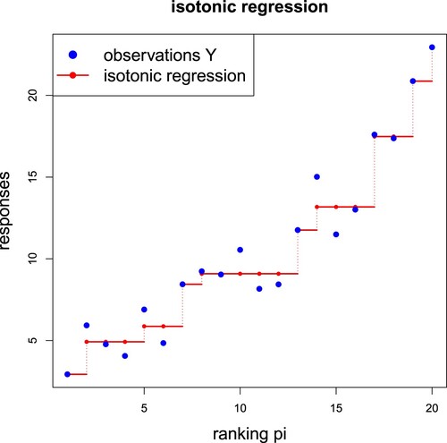
Figure 1 gives an example for n = 20 and rankings $\pi ({\mathit{x}}_i)=i$ for $i=1,\dots ,n$. The resulting (non-parametric) isotonic regression function $\hat{\mathit{\mu }}=\hat{\mathit{\mu }}(\mathit{z})$, which is only uniquely determined at the observations $(\pi ({\mathit{x}}_i){)}_{i=1}^n$, can be interpolated by a step function. In Figure 1 this results in a step function having $K(\mathit{z})-1=9$ steps, that is, we have $K(\mathit{z})=10$ blocks, and the estimated regression function $\hat{\mu }$ takes only $K(\mathit{z})=10$ different values. This motivates to call $K(\mathit{z})$ the complexity number of the resulting step function.

Figure 1. Example of an isotonic regression with $K(\mathit{z})=10$ blocks, the x-axis shows the ranks $(\pi ({\mathit{x}}_i){)}_{i=1}^n$ and the y-axis the resulting isotonic regression estimates $\hat{\mathit{\mu }}$ connected by a step function (in red color).

The partition of the indices $\mathcal{I}$ into the isotonic blocks ${\mathcal{I}}_k$ is obtained naturally by requiring monotonicity. This is different from the regression tree approach considered in Lindholm et al. (2023). In fact, this latter reference does not require monotonicity but aims at minimizing the ‘plain’ square loss using cross-validation for determining the optimal number of partitions. In our context, the complexity number $K(\mathit{z})$ is fully determined through requiring monotonicity and, in general, the results will differ.

In insurance applications, the blocks ${\mathcal{I}}_k\subset \mathcal{I}$ provide us with the (empirical) price cohorts ${\hat{\mu }}_i={\hat{\mu }}_{i_k}$, for $i\in {\mathcal{I}}_k$, and (2.4(2.4) ${\hat{\mu }}_i={\hat{\mu }}_{i_k}=\frac{1}{\sum _{j\in {\mathcal{I}}_k}{w}_j}\sum _{j\in {\mathcal{I}}_k}{w}_j{y}_j,$(2.4) ) leads to the (in-sample) auto-calibration property for Y (2.5) $\mathbb{E}[Y^{\mathrm{\prime }}|\hat{\mu }({\mathit{X}}^{\mathrm{\prime }})={\hat{\mu }}_{i_k}]=\frac{1}{\sum _{i\in {\mathcal{I}}_k}{w}_i}\sum _{i\in {\mathcal{I}}_k}{w}_i{y}_i={\hat{\mu }}_{i_k},$(2.5) where $(Y^{\mathrm{\prime }},{\mathit{X}}^{\mathrm{\prime }})$ is distributed according to the weighted empirical distribution of $(y_i,{\mathit{x}}_i{)}_{i=1}^n$ with weights $(w_i{)}_{i=1}^n$, see also (1.1(1.1) $\hat{\mu }({\mathit{X}}^{\mathrm{\prime }})=\mathbb{E}[Y^{\mathrm{\prime }}|\hat{\mu }({\mathit{X}}^{\mathrm{\prime }})],{\mathbb{P}}_n\text{-a.s.,}$(1.1) ). Moreover, summing over the entire portfolio we have the (global) balance property (2.6) $\sum _{i=1}^n{w}_i{\hat{\mu }}_i=\sum _{k=1}^{K(\mathit{z})}\sum _{i\in {\mathcal{I}}_k}{w}_i{\hat{\mu }}_i=\sum _{k=1}^{K(\mathit{z})}{\hat{\mu }}_{i_k}\sum _{i\in {\mathcal{I}}_k}{w}_i=\sum _{k=1}^{K(\mathit{z})}\sum _{i\in {\mathcal{I}}_k}{w}_i{y}_i=\sum _{i=1}^n{w}_i{y}_i,$(2.6) that is, in average the overall (price) level is correctly specified if we price the insurance policies with covariates ${\mathit{x}}_i$ by $w_i{\hat{\mu }}_i$, where the weights $w_i>0$ now receive the interpretation of exposures.

2.2. Monotonicity of the expected complexity number

In this section, we prove that the expected complexity number $\mathbb{E}[K(\mathit{z})]$ is an increasing function of the signal-to-noise ratio. For this, we assume a location-scale model for the responses $Y_i$, that is, we assume that (2.7) $Y_i={\mu }_i+\sigma {ϵ}_i,i=1,\dots ,n,$(2.7) with noise terms ${ϵ}_i$, location parameters ${\mu }_i\in \mathbb{R}$ with ${\mu }_1\le \cdots \le {\mu }_n$, and scale parameter $\sigma >0$. Here, ${\mu }_i$ takes the role of $\pi ({\mathit{x}}_i)$ in the previous section. The parameters ${\mu }_1,\dots ,{\mu }_n$ are unknown but it is known that they are labeled in increasing order. The signal-to-noise ratio is then described by the scale parameter σ, i.e. we have a low signal-to-noise ratio for high σ and vice-versa. The explicit location-scale structure (2.7(2.7) $Y_i={\mu }_i+\sigma {ϵ}_i,i=1,\dots ,n,$(2.7) ) allows us to analyze (2.8) $\mathit{y}={\mathit{Y}}_{\sigma }(\omega )=\mathit{\mu }+\sigma \mathit{ϵ}(\omega )=({\mu }_1,\dots ,{\mu }_n{)}^{\mathrm{\top }}+\sigma ({ϵ}_1,\dots ,{ϵ}_n{)}^{\mathrm{\top }}(\omega ),$(2.8) point-wise in the sample points $\omega \in \mathrm{\Omega }$ of the probability space $(\mathrm{\Omega },\mathcal{F},\mathbb{P})$ as a function of $\sigma >0$; this is similar to the re-parametrization trick of Kingma & Welling (2019) that is frequently used to explore variational auto-encoders.

In this section, we write $K(\mathit{y})=K(\mathit{z})$, because the ranking of the outcomes $\mathit{y}$ is clear from the context (labeling), and we do not go via a ranking function $\pi (\cdot )$.

Theorem 2.3

Assume that the responses $Y_i$, $i=1,\dots ,n$, follow the location-scale model (2.7(2.7) $Y_i={\mu }_i+\sigma {ϵ}_i,i=1,\dots ,n,$(2.7) ) with (unknown) ordered location parameters ${\mu }_1<\cdots <{\mu }_n$, and scale parameter $\sigma >0$. Then, the expected complexity number $\mathbb{E}[K(\mathit{Y})]$ of the isotonic regression of $\mathit{Y}$ is a decreasing function in $\sigma >0$. If the distribution of the noise vector $\mathit{ϵ}=({ϵ}_1,\dots ,{ϵ}_n{)}^{\mathrm{\top }}$ has full support on ${\mathbb{R}}^n$, then $\mathbb{E}[K(\mathit{Y})]$ is strictly decreasing in σ.

Theorem 2.3 proves that, under a specific but highly relevant model, the complexity number $K(\mathit{Y})$ of the isotonic regression is decreasing on average with a decreasing signal-to-noise ratio. Implicitly, this means that more noisy data, which has a lower information ratio, leads to a less granular regression function. Consequently, if the partition of the isotonic regression is used to obtain a partition of the covariate space $\mathcal{X}$ via the candidate function π, this partition will be less granular, the more noise of $\mathit{Y}$ cannot be explained by $\pi (\mathit{X})$. Remark that ‘explain’ has different meanings in machine learning and in statistics. In statistics, a regression function explains part of the uncertainty in the response variable, also called resolution or discrimination in Murphy's score decomposition (Murphy 1973); see Gneiting & Resin (2022, Theorem 2.23). In our case, a regression function that poorly explains the variability of the response, leads to explainability of the regression function itself by a low complexity partitioning of the covariate space.

To the best of our knowledge, our result is a new contribution to the literature on isotonic regression. While we focus on the finite sample case, a related result studies the complexity number of the isotonic regression function as function of the sample size n, see Dimitriadis et al. (2022, Lemma 3.2). The complexity number is also related to the effective dimension of the model, and has been studied under the assumption of independent Gaussian errors in (2.7(2.7) $Y_i={\mu }_i+\sigma {ϵ}_i,i=1,\dots ,n,$(2.7) ) in Meyer & Woodroofe (2000) and Tibshirani et al. (2011).

We are assuming strictly ordered location parameters ${\mu }_i$ in the formulation of Theorem 2.3. This assumption simplifies the proof in the case where we show that the expected complexity number $K(\mathit{Y})$ is strictly decreasing in σ. With some additional notation, the theorem could be generalized to allow for ties between some (but not all) ${\mu }_i$.

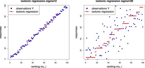
Figure 2 gives an example of a location-scale model (2.7(2.7) $Y_i={\mu }_i+\sigma {ϵ}_i,i=1,\dots ,n,$(2.7) ) with i.i.d. standard Gaussian noise and scale parameters $\sigma =2$ (lhs) and $\sigma =20$ (rhs), and both figures consider the same sample point $\omega \in \mathrm{\Omega }$ in the noise term $\mathit{ϵ}(\omega )$, see (2.8(2.8) $\mathit{y}={\mathit{Y}}_{\sigma }(\omega )=\mathit{\mu }+\sigma \mathit{ϵ}(\omega )=({\mu }_1,\dots ,{\mu }_n{)}^{\mathrm{\top }}+\sigma ({ϵ}_1,\dots ,{ϵ}_n{)}^{\mathrm{\top }}(\omega ),$(2.8) ). On the left-hand side of Figure 2, we have complexity number $K(\mathit{y})=46$, and on the right-hand side $K(\mathit{y})=13$; the chosen sample size is n = 100.

Figure 2. Example of an isotonic regression of location-scale type with varying signal-to-noise ratio for the identical sample point $\omega \in \mathrm{\Omega }$: (lhs) $\sigma =2$ with $K(\mathit{y})=46$ and (rhs) $\sigma =20$ with $K(\mathit{y})=13$.

3. Isotonic recalibration for prediction and interpretation

3.1. Estimation and prediction

To determine an auto-calibrated estimate of the true regression function $\mathit{x}\mapsto \mathbb{E}[Y|\mathit{X}=\mathit{x}]$ from i.i.d. data $(y_i,{\mathit{x}}_i{)}_{i=1}^n$, we are suggesting a two-step estimation procedure. First, we use the data $(y_i,{\mathit{x}}_i{)}_{i=1}^n$ to obtain an estimate $\hat{\pi }$ of a candidate function π that should satisfy (3.1) $\pi (\mathit{x})<\pi ({\mathit{x}}^{\mathrm{\prime }})⟺\mathbb{E}[Y|\mathit{X}=\mathit{x}]<\mathbb{E}[Y|\mathit{X}={\mathit{x}}^{\mathrm{\prime }}],$(3.1) for all $\mathit{x},{\mathit{x}}^{\mathrm{\prime }}\in \mathcal{X}$. This first step is motivated by the fact that the true regression function ${\mu }^{\star }$ is auto-calibrated and satisfies, $\mathbb{P}$-a.s., $\mathbb{E}[Y|\mathit{X}]=:{\mu }^{\star }(\mathit{X})=\mathbb{E}[Y|{\mu }^{\star }(\mathit{X})].$As a consequence, requirement (3.1(3.1) $\pi (\mathit{x})<\pi ({\mathit{x}}^{\mathrm{\prime }})⟺\mathbb{E}[Y|\mathit{X}=\mathit{x}]<\mathbb{E}[Y|\mathit{X}={\mathit{x}}^{\mathrm{\prime }}],$(3.1) ) gives strict comonotonicity between $\pi (\mathit{X})$ and ${\mu }^{\star }(\mathit{X})$, that is, $\mathbb{P}$-a.s., ${\mu }^{\star }(\mathit{X})=T(\pi (\mathit{X}))$ for a strictly increasing function T.

In a second step, we aim at finding this monotone transformation T. We therefore apply isotonic regression (rank-preserving) to the pseudo-sample $(y_i,\hat{\pi }({\mathit{x}}_i){)}_{i=1}^n$ to obtain the in-sample auto-calibrated regression function $\hat{\mu }$ defined on $\{\hat{\pi }({\mathit{x}}_i):i=1,\dots ,n\}$. We call this second step isotonic recalibration, and this isotonically recalibrated version $\hat{\mu }(\mathit{X})$ of $\hat{\pi }(\mathit{X})$ not only satisfies auto-calibration (1.1(1.1) $\hat{\mu }({\mathit{X}}^{\mathrm{\prime }})=\mathbb{E}[Y^{\mathrm{\prime }}|\hat{\mu }({\mathit{X}}^{\mathrm{\prime }})],{\mathbb{P}}_n\text{-a.s.,}$(1.1) ), but it is also an approximation to the true regression function ${\mu }^{\star }(\mathit{X})$, i.e. $\hat{\mu }(\mathit{X})\approx {\mu }^{\star }(\mathit{X})$; for a related statement in a binary classification context we refer to Tasche (2021, Proposition 3.6). In our case study in Section 4, below, a deep neural network model is chosen for estimating the ranks π.

In order to obtain a prediction for a new covariate value $\mathit{x}\in \mathcal{X}$, we compute $\hat{\pi }(\mathit{x})$, find i such that $\hat{\pi }({\mathit{x}}_i)<\hat{\pi }(\mathit{x})\le \hat{\pi }({\mathit{x}}_{i+1})$, and interpolate by setting $\hat{\mu }(\mathit{x})=(\hat{\mu }({\mathit{x}}_i)+\hat{\mu }({\mathit{x}}_{i+1}))/2$. This interpolation may be advantageous for prediction. For interpretation and analysis, however, we prefer a step function interpolation as this leads to a partition of the covariate space, see Section 3.3, below, and Figure 2.

Summarizing, the proposed two-step estimation procedure first aims at getting the ranks $\pi (\mathit{X})$ right, see (3.1(3.1) $\pi (\mathit{x})<\pi ({\mathit{x}}^{\mathrm{\prime }})⟺\mathbb{E}[Y|\mathit{X}=\mathit{x}]<\mathbb{E}[Y|\mathit{X}={\mathit{x}}^{\mathrm{\prime }}],$(3.1) ). Based on a correct ranking, isotonic recalibration lifts these ranks to the right level using that the true regression function ${\mu }^{\star }(\mathit{X})$ is a monotone transformation of the correct ranks $\pi (\mathit{X})$, and, thus, the isotonically recalibrated ranks $\hat{\mu }(\mathit{X})$ provide an approximation to the true regression function ${\mu }^{\star }(\mathit{X})$. A way to verify the rank property (3.1(3.1) $\pi (\mathit{x})<\pi ({\mathit{x}}^{\mathrm{\prime }})⟺\mathbb{E}[Y|\mathit{X}=\mathit{x}]<\mathbb{E}[Y|\mathit{X}={\mathit{x}}^{\mathrm{\prime }}],$(3.1) ) is to maximize the Gini score; we refer to Wüthrich (2023). A first regression function $\pi (\mathit{X})$ may not be auto-calibrated, but since the Gini score is invariant under strictly increasing transformations, maximizing the Gini score is still a valid procedure, if one isotonically recalibrates this first regression function $\pi (\mathit{X})$. As a consequence, isotonic recalibration gives a Gini score preserving transformation that provides the auto-calibrated counterpart of the first regression function. Using the uniqueness part of Theorem 4.3 of Wüthrich (2023) then says that this auto-calibrated version $\hat{\mu }(\mathit{X})$ is a valid approximation to the true regression function. This justifies the isotonic recalibration procedure under (3.1(3.1) $\pi (\mathit{x})<\pi ({\mathit{x}}^{\mathrm{\prime }})⟺\mathbb{E}[Y|\mathit{X}=\mathit{x}]<\mathbb{E}[Y|\mathit{X}={\mathit{x}}^{\mathrm{\prime }}],$(3.1) ), and it is the general regression version of the binary case presented in Menon et al. (2012).

This two-step estimation approach can also be interpreted as a generalization of the monotone single index models considered by Balabdaoui et al. (2019). They assume that the true regression function is of the form $\mathbb{E}[Y|\mathit{X}=\mathit{x}]=\psi ({\mathit{\alpha }}^{\mathrm{\top }}\mathit{x})$, with an increasing function ψ. In contrast to our proposal, the regression model π is fixed to be a linear model ${\mathit{\alpha }}^{\mathrm{\top }}\mathit{x}$ in their approach. They consider global least squares estimation jointly for $(\psi ,\mathit{\alpha })$, but find it computationally intensive. As an alternative they suggest a two-step estimation procedure similar to our approach with a split of the data such that $\mathit{\alpha }$ and the isotonic regression are estimated on independent samples. They find that if the rate of convergence of the estimator for $\mathit{\alpha }$ is sufficiently fast, then the resulting estimator of the true regression function is consistent with a convergence rate of order $n^{1/3}$.

In a distributional regression framework, Henzi et al. (2023) considered the described two-step estimation procedure with an isotonic distributional regression, instead of a classical least squares isotonic regression as described in Section 2.1. They show that in both cases, with and without sample splitting, the procedure leads to consistent estimation of the conditional distribution of Y, given $\mathit{X}$, as long as the index π can be estimated at a parametric rate. The two options, with and without sample splitting, do not result in relevant differences in predictive performance in the applications considered by Henzi et al. (2023).

Assumption (3.1(3.1) $\pi (\mathit{x})<\pi ({\mathit{x}}^{\mathrm{\prime }})⟺\mathbb{E}[Y|\mathit{X}=\mathit{x}]<\mathbb{E}[Y|\mathit{X}={\mathit{x}}^{\mathrm{\prime }}],$(3.1) ) can also be checked by diagnostic plots using binning similarly to the plots in Henzi et al. (2023, Figure 2) in the distributional regression case, such plots are also called lift plots in actuarial practice. Predictive performance should be assessed on a test set of data disjoint from $(y_i,{\mathit{x}}_i{)}_{i=1}^n$, that is, on data that has not been used in the estimation procedure at all. Isotonic recalibration ensures auto-calibration in-sample, and under an i.i.d. assumption, auto-calibration will also hold approximately out-of-sample. Out-of-sample auto-calibration can be diagnosed with CORP (consistent, optimally binned, reproducible and PAV) mean reliability diagrams as suggested by Gneiting & Resin (2022), and comparison of predictive performance can be done with the usual squared error loss function or with deviance loss functions.

3.2. Over-fitting at the boundary

There is a small issue with the isotonic recalibration, namely, it may tend to over-fit at the lower and upper boundaries of the ranks $\hat{\pi }({\mathit{x}}_1)<\cdots <\hat{\pi }({\mathit{x}}_n)$. For instance, if $y_n$ is the largest observation in the portfolio (which is not unlikely since the ranking $\hat{\pi }$ is chosen response data-driven), then we estimate ${\hat{\mu }}_{i_K}=y_n$, where $K=K((y_i,\hat{\pi }({\mathit{x}}_i){)}_{i=1}^n)$. Often, this over-fits to the (smallest and largest) observations, as such extreme values/estimates cannot be verified on out-of-sample data. For this reason, we visually analyze the largest and smallest values in the estimates $\hat{\mathit{\mu }}$, and we manually merge, say, the smallest block ${\mathcal{I}}_1$ with the second smallest one ${\mathcal{I}}_2$ (with the resulting estimate (2.4(2.4) ${\hat{\mu }}_i={\hat{\mu }}_{i_k}=\frac{1}{\sum _{j\in {\mathcal{I}}_k}{w}_j}\sum _{j\in {\mathcal{I}}_k}{w}_j{y}_j,$(2.4) ) on the merged block). More rigorously, this pooling could be cross-validated on out-of-sample data, but we refrain from doing so. In our examples in Section 4.1, below, we merge the two blocks with the smallest/biggest estimates.

3.3. Interpretation

In (2.3(2.3) ${\mathcal{I}}_k={\mathcal{I}}_k(\mathit{z})=\{i_{k-1}+1,\dots ,i_k\}\mathrm{for}k=1,\dots ,K(\mathit{z}),$(2.3) ) we have introduced the complexity number $K((y_i,\hat{\pi }({\mathit{x}}_i){)}_{i=1}^n)$ that counts the number of different values in $\hat{\mathit{\mu }}$, obtained by the isotonic regression (2.2(2.2) $\hat{\mathit{\mu }}=\hat{\mathit{\mu }}(\mathit{z})=\underset{\mathit{\mu }:A\mathit{\mu }\ge \mathbf{0}}{\arg min}(\mathit{y}-\mathit{\mu }{)}^{\mathrm{\top }}W(\mathit{y}-\mathit{\mu }).$(2.2) ) in the isotonic recalibration step. This complexity number $K((y_i,\hat{\pi }({\mathit{x}}_i){)}_{i=1}^n)$ allows one to assess the information content of the model, or in other words, how much signal is explainable from the data. Theorem 2.3 shows that the lower the signal-to-noise ratio, the lower the complexity number of the isotonic regression that we can expect. Clearly, in Theorem 2.3 we assume that the ranking of the observations is correct which will only be approximately satisfied since π has to be estimated. In general, having large samples and flexible regression models for modeling π, it is reasonable to assume that the statement remains qualitatively valid. However, in complex (algorithmic) regression models, we need to ensure that we prevent from in-sample over-fitting; this is typically controlled by either using (independent) validation data or by performing a cross-validation analysis.

Typical claims data in non-life insurance have a low signal-to-noise ratio. Regarding claims frequencies, this low signal-to-noise ratio is caused by the fact that claims are not very frequent events, e.g. in car insurance annual claims frequencies range from 5% to 10%, that is, only one out of 10 (or 20) drivers suffers a claim within a calendar year. A low signal-to-noise ratio also applies to claim amounts, which are usually strongly driven by randomness and the explanatory part from policyholder information is comparably limited. Therefore, we typically expect a low complexity number $K((y_i,\hat{\pi }({\mathit{x}}_i){)}_{i=1}^n)$ both for claims frequency and claim amounts modeling. This low signal-to-noise ratio in actuarial modeling is also a reason for exploiting new sources of information such as telematics data, see, e.g. Peiris et al. (2023), or images, see, e.g. Blier-Wong & Lamontagne (2022).

In case of a small to moderate complexity number $K=K((y_i,\hat{\pi }({\mathit{x}}_i){)}_{i=1}^n)$, the regression function $\hat{\mathit{\mu }}$ becomes interpretable through the isotonic recalibration step. For this, we extend the auto-calibrated regression function $\hat{\mu }$ from the set $\{\hat{\pi }({\mathit{x}}_1),\dots ,\hat{\pi }({\mathit{x}}_n)\}$ to the entire covariate space $\mathcal{X}$ by defining a step function $\hat{\mu }(\mathit{x})={\hat{\mu }}_{i_k},\mathrm{if}\hat{\pi }({\mathit{x}}_{i_k})\le \hat{\pi }(\mathit{x})<\hat{\pi }({\mathit{x}}_{i_{k+1}}),$for all $\mathit{x}\in \mathcal{X}$, where $0=i_0<i_1<\cdots <i_K=n$ are the slicing points of the isotonic regression as defined in (2.3(2.3) ${\mathcal{I}}_k={\mathcal{I}}_k(\mathit{z})=\{i_{k-1}+1,\dots ,i_k\}\mathrm{for}k=1,\dots ,K(\mathit{z}),$(2.3) ). Figure 1 illustrates this step function interpolation. We define a partition ${\mathcal{X}}_1,\dots ,{\mathcal{X}}_K$ of the original covariate space $\mathcal{X}$ by (3.2) ${\mathcal{X}}_k=\{\mathit{x}\in \mathcal{X}:\hat{\mu }(\mathit{x})={\hat{\mu }}_{i_k}\},k=1,\dots ,K.$(3.2) Figure 4, below, illustrates how this partition of $\mathcal{X}$ provides insights on the covariate-response relationships in the model. This procedure has some analogy to regression trees and boosting trees that rely on partitions of the covariate space $\mathcal{X}$. In the case study in Section 4, we illustrate two further possibilities to use the partition defined at (3.2(3.2) ${\mathcal{X}}_k=\{\mathit{x}\in \mathcal{X}:\hat{\mu }(\mathit{x})={\hat{\mu }}_{i_k}\},k=1,\dots ,K.$(3.2) ) for understanding covariate-response relationships. First, in Figure 6, the influence of individual covariates on the price cohorts is analyzed, and second, Figure 7 gives a summary view of the whole covariate space for a chosen price cohort.

Figure 3. Isotonic recalibration in the French MTPL example only using DrivAge and BonusMalus as covariates resulting in the complexity number $K((y_i,\hat{\pi }({\mathit{x}}_i){)}_{i=1}^n)=49$; the x-axis shows the estimated ranks $(\hat{\pi }({\mathit{x}}_i){)}_{i=1}^n$ and the y-axis the resulting isotonic regression estimates $\hat{\mathit{\mu }}$ using a step function (in red color) on $\mathcal{T}$.

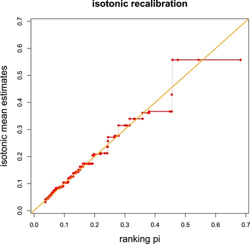
Figure 4. Estimated expected claims frequencies $\hat{\mathit{\mu }}$: (lhs) isotonically recalibrated FFNN regression and (rhs) binary regression tree, both only using DrivAge and BonusMalus as covariates; the color scale shows the expected frequencies, this color scale is the same in both plots.

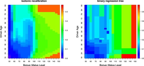
Figure 5. (top-left) Isotonic recalibration, (top-right) regression tree recalibration with 17 leaves, (bottom) local regression recalibration with nearest neighbor fractions $\alpha =5\mathrm{\%},1\mathrm{\%}$ (lhs and rhs); these graphs show how the different recalibration methods change the first FFNN predictions.

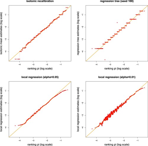
Figure 6. Marginal view of the isotonically recalibrated FFNN predictions (line (2) of Table 2) of the considered covariate components (top) DrivAge, Area, VehPower, (middle) VehAge, BonusMalus, VehGas, (bottom) VehBrand, Region; the K = 77 colors show the distribution of the estimates $\hat{\mathit{\mu }}$ on all levels of the considered covariates.

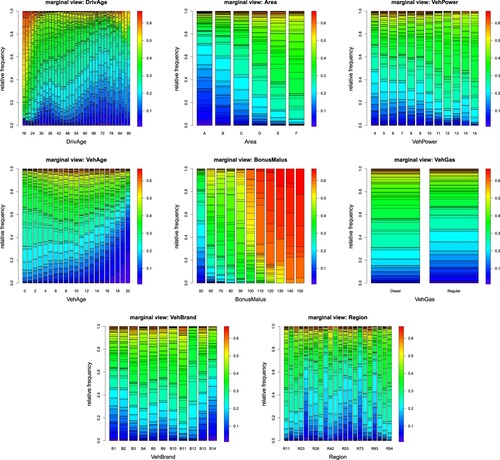
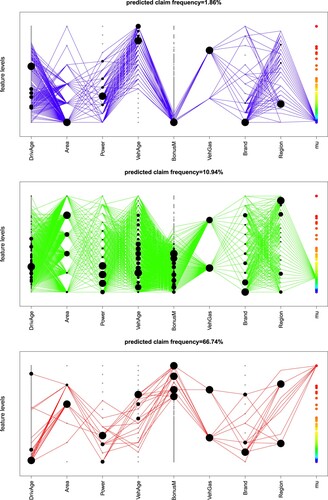
Figure 7. Partition $({\mathcal{X}}_k{)}_{k=1,\dots ,K}$ of the covariate space $\mathcal{X}$ w.r.t. the isotonic recalibration; the complexity number K = 77 induces 77 different expected frequencies illustrated by the colors at the right-hand side of the plots. The lines and dots illustrate the covariate combinations that lead to these expected frequencies for three selected values of k = 2, 45, 77 (top-middle-bottom).

4. Motor third party liability claims frequency example

We consider the French motor third party liability (MTPL) claims frequency data FreMTPL2freq, available through the R package CASdatasets (Dutang & Charpentier 2018). This is a frequently studied dataset that has been considered, e.g. in Lindholm et al. (2023) and Denuit et al. (2021). For an exploratory analysis of this data set we refer to Wüthrich & Merz (2023, Chapter 13). For our analysis we use the same data cleaning as described in Wüthrich & Merz (2023, Listing 13.1), an excerpt of the cleaned data is given in Listing 1.

We have $n=\mathrm{678,007}$ insurance policies which have been exposed within the same accounting year and for which we have claims records and covariate information, see Listing 1. Our goal is to build a neural network regression model for pricing and prediction, and we use isotonic recalibration for auto-calibration and interpretation as described in Section 3.3. To make our analysis directly comparable to the one in Wüthrich & Merz (2023), we partition the available sample into a learning sample $\mathcal{L}$ and a test sample $\mathcal{T}$ precisely as described in Wüthrich & Merz (2023, Listing 5.2). A summary statistics of the resulting learning and test samples is given in Wüthrich & Merz (2023, Table 5.2). For model fitting and the isotonic recalibration step we only use the learning sample $\mathcal{L}$. All models are then evaluated out-of-sample on the test sample $\mathcal{T}$, and these out-of-sample results are directly comparable, e.g. to Wüthrich & Merz (2023, Table 7.10), because we use the identical test sample $\mathcal{T}$.

We remark that in the present study we consider the time exposures as known information for claims frequency modeling. Lindholm et al. (2023) raise the problem of having random time exposures, e.g. caused by early terminations of insurance policies. In some sense, early terminations contaminate claims data which needs a proper statistical treatment for predictive modeling. However, to be able to focus our discussion on isotonic recalibration, we do not discuss and model uncertainties coming from random time exposures here, but we refer to Lindholm et al. (2023) for an in-depth treatment.

4.1. Isotonic recalibration and binary regression trees

We start by considering the two covariate components DrivAge and BonusMalus only. Since the resulting covariate space $\mathcal{X}=\{(\mathtt{\text{DrivAge}},\mathtt{\text{BonusMalus}})\}\subset {\mathbb{R}}^2$ is two-dimensional, we can illustrate graphically the differences between the isotonic recalibration approach and a binary regression tree (as a competing model for interpretation). In Section 4.2, below, we consider all available covariates for a competitive predictive model.

We fit a deep feed-forward neural network (FFNN) regression model to the learning sample $\mathcal{L}$. We choose a network architecture of depth 3 with $(20,15,10)$ neurons in the three hidden layers, the hyperbolic tangent activation function in the hidden layers, and the log-link for the output layer. The input has dimension 2, this results in a FFNN architecture with a network parameter of dimension 546; for a detailed discussion of FFNNs we refer to Wüthrich & Merz (2023, Chapter 7), in particular, to Listings 7.1–7.3 of that reference. We fit this model using the Poisson deviance loss, see Remark 2.2 and Wüthrich & Merz (2023, Section 5.2.4), we use the nadam version of stochastic gradient descent. We exercise early stopping on a validation set being 10% of the learning sample $\mathcal{L}$, and we ensemble over ten different network calibrations to reduce the randomness of individual stochastic gradient descent network fits, see Wüthrich & Merz (2023, Section 7.4.4). Line (1) of Table 1, called ‘FFNN ensemble’, shows the performance of the fitted FFNN regression model ensemble. This is compared to the null model (empirical mean) on line (0) that does not consider any covariates. We observe a decrease in Poisson deviance loss which justifies the use of a regression model. The last column of Table 1, called ‘average frequency’, compares the average frequency estimate of the FFNN ensemble on $\mathcal{L}$ to its empirical mean, and we observe a negative bias in the FFNN prediction, i.e. $7.22\mathrm{\%}<7.36\mathrm{\%}$, thus, these network estimates under-price the portfolio.

Table 1. Loss figures in the French MTPL example only considering DrivAge and BonusMalus; Poisson deviance losses in ${10}^{-2}$.

		Poisson deviance losses
		In-sample	Out-of-sample
		$\mathcal{L}$	$\mathcal{T}$	Average frequency on $\mathcal{L}$
(0)	Null model (empirical mean)	25.213	25.445	7.36%
(1)	FFNN ensemble	24.091	24.160	7.22%
(2)	Isotonic recalibration K = 49	24.073	24.164	7.36%
(3)	Regression tree with 61 leaves	24.066	24.208	7.34%

Table 2. Loss figures in the French MTPL example using all covariates; Poisson deviance losses in ${10}^{-2}$.

		Poisson deviance losses
		In-sample	Out-of-sample
		$\mathcal{L}$	$\mathcal{T}$	Average frequency on $\mathcal{L}$
(0)	Null model (empirical mean)	25.213	25.445	7.36%
(1)	FFNN ensemble	23.716	23.784	7.23%
(2)	Isotonic recalibration, K = 77	23.695	23.800	7.36%
(3)	Tree recalibration, 17 leaves (leaf size ≥100)	23.701	23.811	7.36%
(4a)	Local regression recalibration ($\alpha =0.05$)	23.718	23.806	7.27%
(4b)	Local regression recalibration ($\alpha =0.01$)	23.686	23.818	7.35%

In the next step, we use the FFNN estimates as ranks $\hat{\pi }({\mathit{x}}_i)$ for ordering the claims $y_i$ and the covariates ${\mathit{x}}_i$, respectively. Note that these ranks $\hat{\pi }({\mathit{x}}_i)$ correspond to expected frequencies which still need to be multiplied by the time exposures $w_i>0$ to receive the expected number of claims; these time exposures $w_i>0$ are given on line 3 of Listing 1. Therefore, we perform isotonic recalibration on the observed frequencies for $y_i$. These observed frequencies $y_i$ are obtained by dividing the claim counts, line 13 of Listing 1, by the time exposures, line 3 of Listing 1. Then, the isotonic recalibration step is performed by solving the constraint weighted square loss minimization problem (2.1(2.1) $\hat{\mathit{\mu }}=\underset{\mathit{\mu }=({\mu }_1,\dots ,{\mu }_n{)}^{\mathrm{\top }}}{\arg min}\sum _{i=1}^n{w}_i(y_i-{\mu }_i{)}^2,\text{subject to}{\mu }_1\le \cdots \le {\mu }_n.$(2.1) ) and (2.2(2.2) $\hat{\mathit{\mu }}=\hat{\mathit{\mu }}(\mathit{z})=\underset{\mathit{\mu }:A\mathit{\mu }\ge \mathbf{0}}{\arg min}(\mathit{y}-\mathit{\mu }{)}^{\mathrm{\top }}W(\mathit{y}-\mathit{\mu }).$(2.2) ), respectively. We use the R package monotone (Busing 2022), which provides a fast implementation of the PAV algorithm; in fact, this optimization step takes much less than one second on an ordinary laptop. The numerical results are presented on line (2) of Table 1. We observe that this isotonic recalibration leads to a complexity number $K=K((y_i,\hat{\pi }({\mathit{x}}_i){)}_{i=1}^n)=49$, i.e. we receive a partition into 49 different expected frequencies to represent the isotonically recalibrated FFNN predictor. The out-of-sample loss on $\mathcal{T}$ is slightly increased by this isotonic calibration step, which may indicate that the ranks of the FFNN prediction could be improved. On the other hand, we now have the auto-calibration property (1.1(1.1) $\hat{\mu }({\mathit{X}}^{\mathrm{\prime }})=\mathbb{E}[Y^{\mathrm{\prime }}|\hat{\mu }({\mathit{X}}^{\mathrm{\prime }})],{\mathbb{P}}_n\text{-a.s.,}$(1.1) ) and the global balance property on $\mathcal{L}$, as can be seen from the last column of Table 1.

Figure 3 provides the resulting step function from the isotonic recalibration (in red color) of the ranking $(\hat{\pi }({\mathit{x}}_i){)}_{i=1}^n$ given by the FFNN ensemble. The isotonic recalibration has been performed on $\mathcal{L}$, and Figure 3 shows the results out-of-sample on $\mathcal{T}$. From this figure it is not directly observable why the global balance property does not hold in the first place, as the isotonic recalibration is fairly concentrated around the diagonal orange line.

The isotonic recalibration on the ranks $\hat{\pi }(\mathit{x})=\hat{\pi }(\mathtt{\text{DrivAge}},\mathtt{\text{BonusMalus}})$ of the FFNN leads to a partition ${\mathcal{X}}_1,\dots ,{\mathcal{X}}_{49}$ of the covariate space as defined in (3.2(3.2) ${\mathcal{X}}_k=\{\mathit{x}\in \mathcal{X}:\hat{\mu }(\mathit{x})={\hat{\mu }}_{i_k}\},k=1,\dots ,K.$(3.2) ). We compare this partition to the one that results from a binary split regression tree approach (with Poisson deviance loss). We use 10-fold cross-validation to determine the optimal tree size. In this example the optimal tree has 60 splits and, hence, 61 leaves. The resulting losses of this optimal tree are shown on line (3) of Table 1. We observe that this tree has a worse out-of-sample performance on $\mathcal{T}$ than the isotonically recalibrated version, line (2). The binary regression tree uses a finer partition of the covariate space for this result, 61 leaves vs. complexity number K = 49. Figure 4 which shows the resulting partitions (the color scale illustrates the estimated expected claims frequencies). We observe that binary splitting along the covariate axis may not be sufficiently flexible (the binary tree only has vertical and horizontal splits, see Figure 4, rhs), whereas the isotonically recalibrated version indicates a more complex topology with diagonal splits, see Figure 4 (lhs).

Finally, we remark that the binary tree does not (exactly) fulfill the global balance property, $7.34\mathrm{\%}<7.36\mathrm{\%}$, see last column of Table 1. This comes from the fact that the Poisson binary tree implementation in the R package rpart uses a Bayesian version for frequency estimation to avoid leaves with an expected frequency estimate of zero; see Therneau & Atkinson (2022). In our isotonic recalibration approach, this is avoided by merging the two blocks with the smallest estimates, see Section 3.2.

4.2. Consideration of all covariates

In this section, we consider all available covariate components, see lines 4–12 of Listing 1. We first fit an ensemble of ten FFNNs to the learning sample $\mathcal{L}$. This is done exactly as in the previous section with the only difference that the input dimension changes when we consider all available information. We use the same covariate pre-processing as in Wüthrich & Merz (2023, Example 7.10). That is, we transform the (ordered) Area code to real values, and we use embedding layers of dimension two for the two categorical covariates VehBrand and Region. The FFNN receives a network parameter of dimension 792. The FFNNs are fitted with stochastic gradient descents that are early stopped based on a validation set of 10% of the learning sample $\mathcal{L}$. The results are presented on line (1) of Table 2.

We compare the FFNN prediction to the null model (empirical mean), the FFNN prediction with reduced covariates given in Table 1, and the GLM and network predictors given in Wüthrich & Merz (2023, Tables 5.5 and 7.9). The out-of-sample Poisson deviance losses are directly comparable between all these examples because we use the identical test sample $\mathcal{T}$. In view of these results, we conclude that the FFNN ensemble on line (1) of Table 2 (with an out-of-sample loss of 23.784) is highly competitive because it has roughly the same out-of-sample loss as the best predictor in the aforementioned examples/tables.

Our main concern is the auto-calibration property (1.1(1.1) $\hat{\mu }({\mathit{X}}^{\mathrm{\prime }})=\mathbb{E}[Y^{\mathrm{\prime }}|\hat{\mu }({\mathit{X}}^{\mathrm{\prime }})],{\mathbb{P}}_n\text{-a.s.,}$(1.1) ) and the global balance property (2.6(2.6) $\sum _{i=1}^n{w}_i{\hat{\mu }}_i=\sum _{k=1}^{K(\mathit{z})}\sum _{i\in {\mathcal{I}}_k}{w}_i{\hat{\mu }}_i=\sum _{k=1}^{K(\mathit{z})}{\hat{\mu }}_{i_k}\sum _{i\in {\mathcal{I}}_k}{w}_i=\sum _{k=1}^{K(\mathit{z})}\sum _{i\in {\mathcal{I}}_k}{w}_i{y}_i=\sum _{i=1}^n{w}_i{y}_i,$(2.6) ). We study this on the learning sample $\mathcal{L}$, and in view of the last column of Table 2, we conclude that the FFNN predictor on line (1) severely under-estimates the average frequency, $7.23\mathrm{\%}<7.36\mathrm{\%}$, and auto-calibration fails to hold here.

In the next step, we use the FFNN prediction as ranks $\hat{\pi }({\mathit{x}}_i)$ for ordering the responses and covariates, and we label the claims $y_i$ such that $\hat{\pi }({\mathit{x}}_1)<\cdots <\hat{\pi }({\mathit{x}}_n)$; ties are aggregated as described in Remark 2.1. We then isotonically recalibrate $(\hat{\pi }({\mathit{x}}_i){)}_{i=1}^n$ on the learning sample $\mathcal{L}$. Figure 5 (top-left) shows how the isotonic recalibration step changes the original FFNN predictions (x-axis, on log scale) to their isotonically recalibrated version (y-axis, on log scale). The isotonic recalibration compresses the 581,272 different values of the FFNN predictions to a complexity number of $K=K((y_i,\hat{\pi }({\mathit{x}}_i){)}_{i=1}^n)=77$. Thus, the entire regression problem is encoded (binned) into 77 different estimates ${\hat{\mu }}_{i_k}$, $k=1,\dots ,K$. In view of Figure 5 (top-left), the isotonic recalibration step provides heavier lower and upper tails, and this could also be a sign of over-fitting. This isotonically recalibrated regression is empirically auto-calibrated (2.5(2.5) $\mathbb{E}[Y^{\mathrm{\prime }}|\hat{\mu }({\mathit{X}}^{\mathrm{\prime }})={\hat{\mu }}_{i_k}]=\frac{1}{\sum _{i\in {\mathcal{I}}_k}{w}_i}\sum _{i\in {\mathcal{I}}_k}{w}_i{y}_i={\hat{\mu }}_{i_k},$(2.5) ) on $\mathcal{L}$ and, henceforth, it fulfills the global balance property, see last column of line (2) in Table 2. The resulting out-of-sample loss on $\mathcal{T}$ of 23.800 is slightly worse than the one on line (1) but it is the best of all recalibration methods considered.

We compare the isotonic recalibration results to other recalibration methods, namely, the regression tree binning proposal of Lindholm et al. (2023), and the local regression proposal of Denuit et al. (2021). Both of these methods need hyperparameter tuning which is in contrast to isotonic recalibration. We start with the regression tree recalibration proposed by Lindholm et al. (2023), which aims at finding an optimal binning of the the ranks $\hat{\pi }({\mathit{x}}_1)<\cdots <\hat{\pi }({\mathit{x}}_n)$ using a regression tree predictor. If one would not aim for binning the ranks optimally, but just considered binning, e.g. using empirical deciles, this would result in a ${\chi }^2$-test situation similar to Hosmer & Lemeshow (1980). For an optimal regression tree binning, we use 10-fold cross-validation on $\mathcal{L}$ with the Poisson deviance loss to receive the optimal number of leaves (bins). A further hyperparameter involved is the minimal leaf size, i.e. the required minimal number of instances in each leaf of the regression tree. A comparably small minimal leaf size seems advantageous, and we choose $\ge 100$. Intuitively, this is motivated by the fact that we have ranks $\hat{\pi }({\mathit{x}}_1)<\cdots <\hat{\pi }({\mathit{x}}_n)$ that should respect monotonicity in the true expected frequencies. I.e. though we do not rely on a restricted (isotonic) regression in this tree binning approach, we expect a similar behavior as in the isotonic recalibration because the binary tree splits use this ordering for exploring the best possible splits. If we run 10-fold cross-validation on this configuration, we select an optimal tree size having 17 leaves; there are small variations in this choice because 10-fold cross-validation involves some randomness from the random choice of the folds. The results are presented on line (3) of Table 2 and Figure 5 (top-right).

This tree binning recalibration approach results in a comparably small model, only having 17 leaves, and, in view of Table 2, we have a slightly bigger out-of-sample loss. Interestingly, the regression tree predictor illustrated in Figure 5 (top-right) is not (completely) monotone in the ranks, but there seem to be two outlier bins. There are different explanations for this observation, namely, these outlier bins might be driven by the fact that we have chosen a minimal leaf size that is too small which implies that the irreducible risk (random noise) has a bigger impact on the binary tree splitting, but it could also indicate that the initial ranking of the FFNN predictor is not fully correct in this part of the covariate space. Finally, from the last column of Table 2 we observe that the tree recalibration approach has the global balance property, see line (3); subject to the explanation at the end of Section 4.1 on how rpart treats zeros in predictions; see also Therneau & Atkinson (2022).

The recalibration proposal of Denuit et al. (2021) is based on a local regression; see Loader (1999). This local regression can be interpreted as a local kernel smoothing. Since we use the same data as Denuit et al. (2021), we choose the same configuration for this local regression recalibration as in Denuit et al. (2021, Section 6.1), i.e. based on the R package locfit Loader (1999), we perform a local regression of degree 0 with a nearest neighbor fraction of $\alpha =5\mathrm{\%}$. The results are presented in Figure 5 (bottom-left) and line (4a) of Table 2. This local regression recalibration seems to provide biased estimates in the tails. Selecting a smaller nearest neighbor fraction of $\alpha =1\mathrm{\%}$ gives a smaller bias, but a more wiggly curve in the main body of the data, see Figure 5 (bottom-right), therefore, an adaptive smoothing window size may work better. Focusing on the last column of Table 2, we see that this local regression recalibration tries to accurately estimate the expected frequency locally, but this does not give us any guarantee that the global balance property holds. Alternatively, one could explore a generalized additive model (GAM) which is based on natural cubic splines, and which will have the global balance property if we work with the canonical link.

Next, we exploit Theorem 2.3. The expected claims frequency on the considered data is roughly 7.36%, i.e. we expected that on average only 7 out of 100 car drivers suffer a claim within one calendar year. This is a typical situation of a low signal-to-noise ratio. This can also be verified from Table 2. The total uncertainty of the null model of 25.445 (out-of-sample Poisson deviance loss) is reduced to 23.800 by the regression structure using all available information $\mathit{x}$. Thus, the systematic part reduces the total uncertainty by roughly 6.5%, and the remainder can be interpreted as irreducible risk. This is a typical situation of a low signal-to-noise ratio which, in our case, provides a complexity number of $K((y_i,\hat{\pi }({\mathit{x}}_i){)}_{i=1}^n)=77$, see Figure 5 (top-left); the first FFNN predictor has 581,272 different values. Thus, the resulting complexity of the partition $({\mathcal{X}}_k{)}_{k=1,\dots ,K}$ of the covariate space $\mathcal{X}$ is substantially reduced by the isotonic recalibration. This leads to explainability of insurance prices, illustrated in Figures 6 and 7, that we are going to discuss next.

In Figure 6, we illustrate the resulting marginal plots if we project the estimated values $\hat{\mathit{\mu }}$ of the isotonic recalibration to the corresponding covariate levels, i.e. this is the marginal distribution of the resulting covariate space partition (3.2(3.2) ${\mathcal{X}}_k=\{\mathit{x}\in \mathcal{X}:\hat{\mu }(\mathit{x})={\hat{\mu }}_{i_k}\},k=1,\dots ,K.$(3.2) ) on each level of the considered covariates. For our complexity number of $K((y_i,\hat{\pi }({\mathit{x}}_i){)}_{i=1}^n)=77$, this results in 77 different colors, and the resulting picture can be interpreted nicely, see Figure 6. From this plot we conclude that BonusMalus is the most important covariate component, young DrivAge have significantly higher expected frequencies, Area code A (country side) has a lower expected frequency, etc.

The previous figure gives a marginal view because the estimates (and colors) are projected to the corresponding covariate levels, similar to partial dependence plots (PDPs). Since it is also important to understand interactions of covariate components, we analyze a second plot in Figure 7; this plot uses the same coloring for the 77 different expected frequencies as Figure 6. The lines connect all the covariate combinations in $\mathit{x}$ that are observed within the data $({\mathit{x}}_i{)}_{1\le i\le n}$ for a given value ${\hat{\mu }}_{i_k}$, and the size of the black dots illustrates how often a certain covariate level is represented in this data. E.g. the figure on the top belongs to the second smallest expected claims frequency estimate ${\hat{\mu }}_{i_2}=1.86\mathrm{\%}$. These car drivers are aged above 30, they mostly live in Area A, have lower power and old cars, and they are on the lowest bonus-malus level. The bottom plot shows the drivers that belong to the biggest expected frequency of ${\hat{\mu }}_{i_2}=66.74\mathrm{\%}$. Not surprisingly, these are mostly young drivers (and some very old drivers) with a higher bonus-malus level. Similar conclusions can be drawn for the other parts ${\mathcal{X}}_k$ of the covariate space $\mathcal{X}$, thus, having a low complexity number $K((y_i,\hat{\pi }({\mathit{x}}_i){)}_{i=1}^n)$ enables to explain the regression model.

Finally, we perform a robustness check of the isotonic recalibration by perturbing the ranks $(\hat{\pi }({\mathit{x}}_i){)}_{i=1}^n$. As a benchmark, we consider the local regression calibration to which we apply the same perturbations. In a first experiment, we choose a different FFNN ensemble. Since network fitting involves several elements of randomness, see Wüthrich & Merz (2023, Remarks 7.9), every fitted network will be slightly different. On lines (2a)–(2c) of Table 3, we consider a second FFNN ensemble to which we apply precisely the same isotonic recalibration and local regression recalibration (using the same hyperparameters) as to the first one on lines (1a)-(1c). The results are rather similar which supports a certain robustness across different FFNN calibrations. The second experiment that we consider is to randomly locally perturb the ranks $(\hat{\pi }({\mathit{x}}_i){)}_{i=1}^n$ of the first FFNN ensemble by multiplying the estimated FFNN frequencies by $1+20\mathrm{\%}\cdot (2U_i-1)$ for i.i.d. standard uniformly distributed random variables $U_i$. This increases or decreases to original frequencies by maximally $20\mathrm{\%}$. Through this additional random noise we generally expect that the complexity number K will decrease. The results are presented on lines (3a)–(3c). We observe that this perturbation does not harm the results too much, which supports that these methods have a certain robustness towards small perturbations of the ranks.

Table 3. Robustness check in the French MTPL example using all covariates; Poisson deviance losses in ${10}^{-2}$.

		Poisson deviance losses
		In-sample	Out-of-sample
		$\mathcal{L}$	$\mathcal{T}$	Average frequency on $\mathcal{L}$
(0)	Null model (empirical mean)	25.213	25.445	7.36%
(1a)	1st FFNN ensemble	23.716	23.784	7.23%
(1b)	Isotonic recalibration K = 77	23.695	23.800	7.36%
(1c)	Local regression recalibration ($\alpha =0.05$)	23.718	23.806	7.27%
(2a)	2nd FFNN ensemble	23.707	23.774	7.23%
(2b)	Isotonic recalibration K = 74	23.685	23.790	7.36%
(2c)	Local regression recalibration ($\alpha =0.05$)	23.706	23.793	7.27%
(3a)	Perturbed FFNN ensemble	23.772	23.819	7.23%
(3b)	Isotonic recalibration K = 72	23.749	23.813	7.36%
(3c)	Local regression recalibration ($\alpha =0.05$)	23.767	23.830	7.27%

5. Conclusions

We have tackled two problems. First, we have enforced that the regression model fulfills the auto-calibration property by applying an isotonic recalibration to the ranks of a fitted (first) regression model. This isotonic recalibration does not involve any hyperparameters, but it solely assumes that the ranks from the first regression model are (approximately) correct. Isotonic regression has the property that the complexity of the resulting (non-parametric) regression function is small in low signal-to-noise ratio problems. Benefiting from this property, we have shown that this leads to explainable regression functions because a low complexity is equivalent to a coarse partition of the covariate space. In insurance pricing problems, this is particularly useful as we typically face a low signal-to-noise ratio in insurance claims data. We can then fit a complex (algorithmic) model to that data in a first step, and in a subsequent step we propose to auto-calibrate the first regression function using isotonic recalibration, which also leads to a substantial simplification of the regression function.

Acknowledgements

We would like thank the editor and the referees for giving us very useful remarks that have helped us to improve this manuscript. The second author would like to thank Alexander Henzi for pointing out related results on the complexity number of isotonic regression.

Disclosure statement

No potential conflict of interest was reported by the author(s).

Appendix

A.1. Pool adjacent violators algorithm

Minimization problem (2.2(2.2) $\hat{\mathit{\mu }}=\hat{\mathit{\mu }}(\mathit{z})=\underset{\mathit{\mu }:A\mathit{\mu }\ge \mathbf{0}}{\arg min}(\mathit{y}-\mathit{\mu }{)}^{\mathrm{\top }}W(\mathit{y}-\mathit{\mu }).$(2.2) ) is a quadratic optimization problem with linear side constraints, and it can be solved using the method of Karush–Kuhn–Tucker (KKT) (Karush 1939, Kuhn & Tucker 1951). We therefore consider the Lagrangian $L(\mathit{\mu },\mathit{\eta })=(\mathit{y}-\mathit{\mu }{)}^{\mathrm{\top }}W(\mathit{y}-\mathit{\mu })-{\mathit{\eta }}^{\mathrm{\top }}A\mathit{\mu },$with Lagrange multiplier $\mathit{\eta }\in {\mathbb{R}}^{n-1}$. The KKT conditions are given by (A1) $\begin{array}{rl}\mathbf{0}& ={\mathrm{\nabla }}_{\mathit{\mu }}L(\mathit{\mu },\mathit{\eta })=-W(\mathit{y}-\mathit{\mu })-A^{\mathrm{\top }}\mathit{\eta },\end{array}$(A1) (A2) $\begin{array}{rl}\mathbf{0}& \ge {\mathrm{\nabla }}_{\mathit{\eta }}L(\mathit{\mu },\mathit{\eta })=-A\mathit{\mu },\end{array}$(A2) (A3) $\begin{array}{rl}\mathbf{0}& \le \mathit{\eta },\end{array}$(A3) (A4) $\begin{array}{rl}\mathbf{0}& =({\eta }_1({\mu }_1-{\mu }_2),\dots ,{\eta }_{n-1}({\mu }_{n-1}-{\mu }_n){)}^{\mathrm{\top }}.\end{array}$(A4) The solution to these KKT conditions (A1(A1) $\begin{array}{rl}\mathbf{0}& ={\mathrm{\nabla }}_{\mathit{\mu }}L(\mathit{\mu },\mathit{\eta })=-W(\mathit{y}-\mathit{\mu })-A^{\mathrm{\top }}\mathit{\eta },\end{array}$(A1) )–(A4(A4) $\begin{array}{rl}\mathbf{0}& =({\eta }_1({\mu }_1-{\mu }_2),\dots ,{\eta }_{n-1}({\mu }_{n-1}-{\mu }_n){)}^{\mathrm{\top }}.\end{array}$(A4) ) provides the isotonic estimate $\hat{\mathit{\mu }}$. This solution can be found by the PAV algorithm. The main idea is to compare raw estimates $({\tilde{\mu }}_i{)}_i$. If we have an adjacent pair with ${\tilde{\mu }}_i>{\tilde{\mu }}_{i+1}$, it violates the monotonicity constraint. Such pairs are recursively merged (pooled) to a block with an identical estimate, and iterating this pooling of adjacent pairs and blocks, respectively, that violate the monotonicity constraint, yields the PAV algorithm.

Pool Adjacent Violators (PAV) Algorithm

(0)	Initialize the algorithm ${\hat{\mathit{\mu }}}^{(0)}=\mathit{y}$ and define the blocks ${\mathcal{I}}_k^{(0)}=\{k\}$ for $k=1,\dots ,K^{(0)}=n$.
(1)	Iterate for $t\ge 0$: If ${\hat{\mathit{\mu }}}^{(t)}$ fulfills KKT condition (A2(A2) $\begin{array}{rl}\mathbf{0}& \ge {\mathrm{\nabla }}_{\mathit{\eta }}L(\mathit{\mu },\mathit{\eta })=-A\mathit{\mu },\end{array}$(A2) ) go to item (2), otherwise go to the next step (1b). Select an index $i=1,\dots ,n$ with ${\hat{\mu }}_i^{(t)}>{\hat{\mu }}_{i+1}^{(t)}$, merge the two adjacent blocks with $i\in {\mathcal{I}}_k^{(t)}$ and $i+1\in {\mathcal{I}}_{k+1}^{(t)}$, and leave all other blocks unchanged. This provides the new blocks ${\mathcal{I}}_k^{(t+1)}$ with $k=1,\dots ,K^{(t+1)}=K^{(t)}-1$. Set on each block $k=1,\dots ,K^{(t+1)}$ and for all indices $i\in {\mathcal{I}}_k^{(t+1)}$ the new estimates (A5) ${\hat{\mu }}_i^{(t+1)}=\frac{1}{\sum _{j\in {\mathcal{I}}_k^{(t+1)}}{w}_j}\sum _{j\in {\mathcal{I}}_k^{(t+1)}}{w}_j{y}_j.$(A5) Increase $t\mapsto t+1$.
(2)	Set the isotonic regression estimate $\hat{\mathit{\mu }}={\hat{\mathit{\mu }}}^{(t)}$ and merge adjacent blocks ${\mathcal{I}}_k^{(t)}$ and ${\mathcal{I}}_{k+1}^{(t)}$ if we have the same estimates ${\hat{\mu }}_i$ on these blocks. Return the resulting partition of $\mathcal{I}$ denoted by $({\mathcal{I}}_k{)}_{k=1,\dots ,K}$ and $\hat{\mathit{\mu }}$.

Remark A.1

PAV algorithm interpretation

1. We initialize with the unconstraint optimal solution, and setting ${\mathit{\eta }}^{(0)}=0$ ensures that the KKT conditions (A1(A1) $\begin{array}{rl}\mathbf{0}& ={\mathrm{\nabla }}_{\mathit{\mu }}L(\mathit{\mu },\mathit{\eta })=-W(\mathit{y}-\mathit{\mu })-A^{\mathrm{\top }}\mathit{\eta },\end{array}$(A1) ), (A3(A3) $\begin{array}{rl}\mathbf{0}& \le \mathit{\eta },\end{array}$(A3) ) and (A4(A4) $\begin{array}{rl}\mathbf{0}& =({\eta }_1({\mu }_1-{\mu }_2),\dots ,{\eta }_{n-1}({\mu }_{n-1}-{\mu }_n){)}^{\mathrm{\top }}.\end{array}$(A4) ) are fulfilled, thus, only the monotonicity (A2(A2) $\begin{array}{rl}\mathbf{0}& \ge {\mathrm{\nabla }}_{\mathit{\eta }}L(\mathit{\mu },\mathit{\eta })=-A\mathit{\mu },\end{array}$(A2) ) is not necessarily fulfilled.

   1. We identify a pair ${\hat{\mu }}_i^{(t)}>{\hat{\mu }}_{i+1}^{(t)}$ that violates the monotonicity constraint (A2(A2) $\begin{array}{rl}\mathbf{0}& \ge {\mathrm{\nabla }}_{\mathit{\eta }}L(\mathit{\mu },\mathit{\eta })=-A\mathit{\mu },\end{array}$(A2) ). This pair needs to belong to two adjacent blocks ${\mathcal{I}}_k^{(t)}$ and ${\mathcal{I}}_{k+1}^{(t)}$ because within blocks we have constant estimates (2.4(2.4) ${\hat{\mu }}_i={\hat{\mu }}_{i_k}=\frac{1}{\sum _{j\in {\mathcal{I}}_k}{w}_j}\sum _{j\in {\mathcal{I}}_k}{w}_j{y}_j,$(2.4) ). We merge these two adjacent blocks to ${\mathcal{I}}_k^{(t+1)}={\mathcal{I}}_k^{(t)}\cup {\mathcal{I}}_{k+1}^{(t)}$, which reduces the number of blocks $K^{(t)}$ by 1.

   2. We set on each block the constant estimate (A5(A5) ${\hat{\mu }}_i^{(t+1)}=\frac{1}{\sum _{j\in {\mathcal{I}}_k^{(t+1)}}{w}_j}\sum _{j\in {\mathcal{I}}_k^{(t+1)}}{w}_j{y}_j.$(A5) ) which satisfies the monotonicity constraint (A2(A2) $\begin{array}{rl}\mathbf{0}& \ge {\mathrm{\nabla }}_{\mathit{\eta }}L(\mathit{\mu },\mathit{\eta })=-A\mathit{\mu },\end{array}$(A2) ) within blocks, and also (A4(A4) $\begin{array}{rl}\mathbf{0}& =({\eta }_1({\mu }_1-{\mu }_2),\dots ,{\eta }_{n-1}({\mu }_{n-1}-{\mu }_n){)}^{\mathrm{\top }}.\end{array}$(A4) ) is naturally fulfilled in this block. Conditions (A1(A1) $\begin{array}{rl}\mathbf{0}& ={\mathrm{\nabla }}_{\mathit{\mu }}L(\mathit{\mu },\mathit{\eta })=-W(\mathit{y}-\mathit{\mu })-A^{\mathrm{\top }}\mathit{\eta },\end{array}$(A1) ) and (A3(A3) $\begin{array}{rl}\mathbf{0}& \le \mathit{\eta },\end{array}$(A3) ) are achieved by changing the Lagrange parameter ${\mathit{\eta }}^{(t)}\mapsto {\mathit{\eta }}^{(t+1)}\ge \mathbf{0}$ correspondingly to account for the change in mean estimates (A5(A5) ${\hat{\mu }}_i^{(t+1)}=\frac{1}{\sum _{j\in {\mathcal{I}}_k^{(t+1)}}{w}_j}\sum _{j\in {\mathcal{I}}_k^{(t+1)}}{w}_j{y}_j.$(A5) ) in (A1(A1) $\begin{array}{rl}\mathbf{0}& ={\mathrm{\nabla }}_{\mathit{\mu }}L(\mathit{\mu },\mathit{\eta })=-W(\mathit{y}-\mathit{\mu })-A^{\mathrm{\top }}\mathit{\eta },\end{array}$(A1) ).

   3. On a sample of size n, this algorithm can be iterated at most n−1 times, thus, the algorithm will terminate.

2. Since we have for $i\in {\mathcal{I}}_k^{(t)}$ and $i+1\in {\mathcal{I}}_{k+1}^{(t)}$ the inequality ${\hat{\mu }}_i^{(t)}\le {\hat{\mu }}_{i+1}^{(t)}$, the last step is to ensure that the resulting blocks are maximal by merging blocks where we do not have a strict inequality in the corresponding estimates.

A.2. Proof of Theorem 2.3

Proof

Proof of Theorem 2.3

For given responses $\mathit{y}={\mathit{Y}}_{\sigma }(\omega )$, the solution to (2.2(2.2) $\hat{\mathit{\mu }}=\hat{\mathit{\mu }}(\mathit{z})=\underset{\mathit{\mu }:A\mathit{\mu }\ge \mathbf{0}}{\arg min}(\mathit{y}-\mathit{\mu }{)}^{\mathrm{\top }}W(\mathit{y}-\mathit{\mu }).$(2.2) ) gives the partition (2.3(2.3) ${\mathcal{I}}_k={\mathcal{I}}_k(\mathit{z})=\{i_{k-1}+1,\dots ,i_k\}\mathrm{for}k=1,\dots ,K(\mathit{z}),$(2.3) ) of the index set $\mathcal{I}$ with empirical weighted averages (2.4(2.4) ${\hat{\mu }}_i={\hat{\mu }}_{i_k}=\frac{1}{\sum _{j\in {\mathcal{I}}_k}{w}_j}\sum _{j\in {\mathcal{I}}_k}{w}_j{y}_j,$(2.4) ) on the blocks ${\mathcal{I}}_k$. These empirical weighted averages satisfy ${\hat{\mu }}_{i_k}<{\hat{\mu }}_{i_{k+1}}$ for all $k=1,\dots ,K(\mathit{Y})-1$, because the blocks ${\mathcal{I}}_k$ have been chosen maximal. We now consider how these blocks are constructed in the PAV algorithm. Suppose that we are in iteration $t\ge 0$, and in this iteration of the PAV algorithm, we merge the two adjacent blocks ${\mathcal{I}}_k^{(t)}$ and ${\mathcal{I}}_{k+1}^{(t)}$ because ${\hat{\mu }}_i^{(t)}>{\hat{\mu }}_{i+1}^{(t)}$ for $i\in {\mathcal{I}}_k^{(t)}$ and $i+1\in {\mathcal{I}}_{k+1}^{(t)}$. We analyze this inequality $\frac{1}{\sum _{j\in {\mathcal{I}}_k^{(t)}}{w}_j}\sum _{j\in {\mathcal{I}}_k^{(t)}}{w}_j{y}_j={\hat{\mu }}_i^{(t)}>{\hat{\mu }}_{i+1}^{(t)}=\frac{1}{\sum _{l\in {\mathcal{I}}_{k+1}^{(t)}}{w}_l}\sum _{l\in {\mathcal{I}}_{k+1}^{(t)}}{w}_l{y}_l.$We use the location-scale structure (2.4(2.4) ${\hat{\mu }}_i={\hat{\mu }}_{i_k}=\frac{1}{\sum _{j\in {\mathcal{I}}_k}{w}_j}\sum _{j\in {\mathcal{I}}_k}{w}_j{y}_j,$(2.4) ) which gives us the equivalent condition $\frac{1}{\sum _{j\in {\mathcal{I}}_k^{(t)}}{w}_j}\sum _{j\in {\mathcal{I}}_k^{(t)}}{w}_j({\mu }_j+\sigma {ϵ}_j(\omega ))>\frac{1}{\sum _{l\in {\mathcal{I}}_{k+1}^{(t)}}{w}_l}\sum _{l\in {\mathcal{I}}_{k+1}^{(t)}}{w}_l({\mu }_l+\sigma {ϵ}_l(\omega )).$Since for any indices $j\in {\mathcal{I}}_k^{(t)}$ and $l\in {\mathcal{I}}_{k+1}^{(t)}$ we have ${\mu }_j\le {\mu }_l$, it follows that the previous condition for merging the two adjacent blocks ${\mathcal{I}}_k^{(t)}$ and ${\mathcal{I}}_{k+1}^{(t)}$ in iteration t of the PAV algorithm reads as (A6) $\sigma [\frac{\sum _{j\in {\mathcal{I}}_k^{(t)}}{w}_j{ϵ}_j(\omega )}{\sum _{j\in {\mathcal{I}}_k^{(t)}}{w}_j}-\frac{\sum _{l\in {\mathcal{I}}_{k+1}^{(t)}}{w}_l{ϵ}_l(\omega )}{\sum _{l\in {\mathcal{I}}_{k+1}^{(t)}}{w}_l}]>\frac{\sum _{l\in {\mathcal{I}}_{k+1}^{(t)}}{w}_l{\mu }_l}{\sum _{l\in {\mathcal{I}}_{k+1}^{(t)}}{w}_l}-\frac{\sum _{j\in {\mathcal{I}}_k^{(t)}}{w}_j{\mu }_j}{\sum _{j\in {\mathcal{I}}_k^{(t)}}{w}_j}\ge 0.$(A6) The important observation is that if this condition is fulfilled for scale parameter $\sigma >0$, then it will also be fulfilled for any bigger scale parameter ${\sigma }^{\mathrm{\prime }}>\sigma >0$ (pointwise in $\omega \in \mathrm{\Omega }$). Thus, any pooling that happens for σ also happens for ${\sigma }^{\mathrm{\prime }}>\sigma >0$. Since this is pointwise on the underlying probability space $(\mathrm{\Omega },\mathcal{F},\mathbb{P})$, it shows that $\mathbb{E}[K(\mathit{Y})]$ is decreasing in $\sigma >0$.

Suppose now that the distribution of $\mathit{ϵ}$ has full support on ${\mathbb{R}}^n$. Then, the event $A_{\sigma }=\{K({\mathit{Y}}_{\sigma })=n\}$ occurs with positive probability, i.e. $\begin{array}{rl}0& <\mathbb{P}[A_{\sigma }]=\mathbb{P}[K({\mathit{Y}}_{\sigma })=n]\\ & =\mathbb{P}[Y_1<Y_2<\cdots <Y_n]\\ & =\mathbb{P}[{\mu }_1+\sigma {ϵ}_1<{\mu }_2+\sigma {ϵ}_2<\cdots <{\mu }_n+\sigma {ϵ}_n].\end{array}$Consider $\begin{array}{rl}{A}_{\sigma }& =\{{\mu }_1+\sigma {ϵ}_1<{\mu }_2+\sigma {ϵ}_2<\cdots <{\mu }_n+\sigma {ϵ}_n\}\\ & =\bigcap _{k=2}^n\{{\mu }_{k-1}+\sigma {ϵ}_{k-1}<{\mu }_k+\sigma {ϵ}_k\}\\ & =\{\sigma ({ϵ}_1-{ϵ}_2)<{\mu }_2-{\mu }_1\}\cap \bigcap _{k=3}^n\{{\mu }_{k-1}+\sigma {ϵ}_{k-1}<{\mu }_k+\sigma {ϵ}_k\}.\end{array}$We focus on the first event on the right-hand side. Note that ${\mu }_2-{\mu }_1>0$, hence ${\tilde{A}}_{\sigma }=\{\mathit{\epsilon }\in {\mathbb{R}}^n:{\epsilon }_1-{\epsilon }_2<\frac{{\mu }_2-{\mu }_1}{\sigma }\}$describes an open half space in ${\mathbb{R}}^n$ containing the origin and with bounding hyperplane that moves further away from the origin when decreasing σ. Overall, the set ${\tilde{A}}_{\sigma }\subset {\mathbb{R}}^n$ of values of $\mathit{\epsilon }$ is a non-empty open polyhedron containing the origin that scales with σ, that is, ${\tilde{A}}_{\sigma }=(1/\sigma ){\tilde{A}}_1$. Therefore, since the distribution of $\mathit{ϵ}$ has full support, the probability $\mathbb{P}[A_{\sigma }]$ is strictly decreasing in σ.

References

- Ayer, M., Brunk, H. D., Ewing, G. M., Reid, W. T. & Silverman, E. (1955). An empirical distribution function for sampling with incomplete information. Annals of Mathematical Statistics 26, 641–647.
- Balabdaoui, F., Durot, C. & Jankowski, H. (2019). Least squares estimation in the monotone single index model. Bernoulli 25, 3276–3310.
- Barlow, R. E., Bartholomew, D. J., Brenner, J. M. & Brunk, H. D. (1972). Statistical inference under order restrictions. Wiley.
- Barlow, R. E. & Brunk, H. D. (1972). The isotonic regression problem and its dual. Journal of the American Statistical Association 67(337), 140–147.
- Blier-Wong, C., Lamontagne, L. & Marceau, E. (2022). A representation-learning approach for insurance pricing with images. Insurance Data Science Conference, 15–17 June 2022, Milan.
- Brunk, H. D., Ewing, G. M. & Utz, W. R. (1957). Minimizing integrals in certain classes of monotone functions. Pacific Journal of Mathematics 7, 833–847.
- Busing, F. M. T. A. (2022). Monotone regression: a simple and fast O(n) PAVA implementation. Journal of Statistical Software 102, 1–25.
- de Leeuw, J., Hornik, K. & Mair, P. (2009). Isotone optimization in R: pool-adjacent-violators algorithm (PAVA) and active set methods. Journal of Statistical Software 32(5), 1–24.
- Denuit, M., Charpentier, A. & Trufin, J. (2021). Autocalibration and Tweedie-dominance for insurance pricing with machine learning. Insurance: Mathematics & Economics 101, 485–497.
- Dimitriadis, T., Dümbgen, L., Henzi, A., Puke, M. & Ziegel, J. (2022). Honest calibration assessment for binary outcome predictions. arXiv:2203.04065.
- Dutang, C. & Charpentier, A. (2018). CASdatasets R Package Vignette. Reference Manual. Version 1.0-8, packaged 2018-05-20.
- Gneiting, T. (2011). Making and evaluating point forecasts. Journal of the American Statistical Association 106(494), 746–762.
- Gneiting, T. & Resin, J. (2022). Regression diagnostics meets forecast evaluation: conditional calibration, reliability diagrams and coefficient of determination. arXiv:2108.03210v3.
- Henzi, A., Kleger, G.-R. & Ziegel, J. F. (2023). Distributional (single) index models. Journal of the American Statistical Association 118(541), 489–503.
- Henzi, A., Ziegel, J. F. & Gneiting, T. (2021). Isotonic distributional regression. Journal of the Royal Statistical Society Series B: Statistical Methodology 83, 963–993.
- Hosmer, D. W. & Lemeshow, S. (1980). Goodness of fit tests for the multiple logistic regression model. Communications in Statistics - Theory and Methods 9, 1043–1069.
- Karush, W. (1939). Minima of functions of several variables with inequalities as side constraints [MSc thesis]. Department of Mathematics, University of Chicago.
- Kingma, D. P. & Welling, M. (2019). An introduction to variational autoencoders. Foundations and Trends in Machine Learning 12(4), 307–392.
- Krüger, F. & Ziegel, J. F. (2021). Generic conditions for forecast dominance. Journal of Business & Economics Statistics 39(4), 972–983.
- Kruskal, J. B. (1964). Nonmetric multidimensional scaling: a numerical method. Psychometrika 29, 115–129.
- Kuhn, H. W. & Tucker, A. W. (1951). Nonlinear programming. Proceedings of 2nd Berkeley Symposium. University of California Press. P. 481–492.
- Lindholm, M., Lindskog, F. & Palmquist, J. (2023). Local bias adjustment, duration-weighted probabilities, and automatic construction of tariff cells. Scandinavian Actuarial Journal, published online: 14 Feb 2023.
- Loader, C. (1999). Local regression and likelihood. Springer.
- Lundberg, S. M. & Lee, S.-I. (2017). A unified approach to interpreting model predictions. In Advances in Neural Information Processing Systems 30. Guyon, I., Luxburg, U.V., Bengio, S., Wallach, H., Fergus, R., Vishwanathan, S., Garnett, R. (Eds.). Curran Associates. P. 4765–4774.
- Mayer, M., Meier, D. & Wüthrich, M. V. (2023). SHAP for actuaries: explain any model. SSRN Manuscript ID 4389797.
- Menon, A. K., Jiang, X., Vembu, S., Elkan, C. & Ohno-Machado, L. (2012). Predicting accurate probabilities with ranking loss. ICML'12: Proceedings of the 29th International Conference on Machine Learning. Omnipress, 2600 Anderson Street, Madison, WI, United States P. 659–666.
- Meyer, M. & Woodroofe, M. (2000). On the degrees of freedom in shape-restricted regression. Annals of Statistics 28(4), 1083–1104.
- Miles, R. E. (1959). The complete amalgamation into blocks, by weighted means, of a finite set of real numbers. Biometrika 46, 317–327.
- Murphy, A. H. (1973). A new vector partition of the probability score. Journal of Applied Meteorology 12(4), 595–600.
- Peiris, H., Jeong, H. & Kim, J.-K. (2023). Integration of traditional and telematics data for efficient insurance claims prediction. SSRN Manuscript ID 4344952.
- Savage, L. J. (1971). Elicitable of personal probabilities and expectations. Journal of the American Statistical Association 66(336), 783–801.
- Schervish, M. J. (1989). A general method of comparing probability assessors. The Annals of Statistics 17(4), 1856–1879.
- Tasche, D. (2021). Calibrating sufficiently. Statistics: A Journal of Theoretical and Applied Statistics 55(6), 1356–1386.
- Therneau, T. M. & Atkinson, E. J. (2022). An introduction to recursive partitioning using the RPART routines. R Vignettes, version of October 21, 2022. Rochester: Mayo Foundation.
- Tibshirani, R. J., Hoefling, H. & Tibshirani, R. (2011). Nearly-isotonic regression. Technometrics 53(1), 54–61.
- Wüthrich, M. V. (2023). Model selection with Gini indices under auto-calibration. European Actuarial Journal 13(1), 469–477.
- Wüthrich, M. V. & Merz, M. (2023). Statistical foundations of actuarial learning and its applications. Springer Actuarial.
- Zadrozny, B. & Elkan, C. (2002). Transforming classifier scores into accurate multiclass probability estimates. Proceedings of the Eighth ACM SIGKDD International Conference on Knowledge Discovery and Data Mining. Association for Computing Machinery, New York, NY, United State P. 694–699.