Cashflow-driven investment beyond expectations

ABSTRACT

This paper presents a computationally tractable optimization model for cashflow-driven investment where the aim is to find asset portfolios whose future payouts cover given liability payments as well as possible. While current industry solutions are largely based on expected future cash flows, we use a stochastic optimization model that seeks portfolios that give the best possible match across time as well as scenarios. Cashflow matching across scenarios is controlled by risk aversion while the timing is driven by illiquidity of money markets. When illiquidity increases, the hedging strategy quickly shifts towards portfolios suggested by deterministic models, but significant uncertainty remains. The model can incorporate hundreds of quoted instruments in the construction of optimal hedging strategies. The hedging strategies are able to employ any statistical connections between the liabilities and publicly quoted assets. The model is solved with simple Monte Carlo approximations and off-the-shelf convex optimization software. Besides optimal hedging strategies, we find the least cost of hedging which provides a market-consistent valuation based on the current quotes and the liquidity factors as well as the views and risk preferences of the investor/regulator. The approach is illustrated by pricing and hedging defined benefit pension liabilities which depend on uncertain longevity developments and the consumer price index. The hedging strategies are constructed from 128 publicly quoted instruments including index-linked bonds and equities. We find that the optimized hedging strategies achieve lower risk at a lower cost than the strategies obtained by matching expected cashflows. The hedging-based liability valuations are robust with respect to model parameters and the additional risk reduction achieved by optimization does not add much to the overall hedging cost.

KEYWORDS:

• Asset-liability management
• cashflow-driven investment
• convex stochastic optimization
• defined benefit pensions

1. Introduction

Cashflow-driven investment (CDI) has become a recommended approach e.g. for defined benefit (DB) pension funds who face an outflow of cash over the coming decades; see Heaven et al. (n.d.), Watson (2019), Pensions and Lifetime Savings Association (2019), Institute and Faculty of Actuaries (2019), Exley (2017), Kazziha et al. (2019), Mcinally (2019), and Insight Investment (n.d.) for a small sample of practitioner-oriented papers. A CDI portfolio aims to cover the pension payments with the contractual payments of the involved assets when held to maturity. If one could achieve perfect cashflow matching, such a portfolio would provide the security of delivering liability payments without exposure to market or longevity risk or to reinvestment risks associated with future trading. This would be ideal for large DB schemes that face significant liquidity risks that may be difficult to control with dynamic asset allocation. Many traditional ALM approaches such as duration matching and liability-driven investment (LDI) aim at matching valuations of liabilities with valuations of assets so they are sensitive to the employed valuation principles which often have little to do with the true costs of delivering the cashflows. CDI can be seen as an economically consistent ALM technique as it focuses on the actual delivery of the liability payments.

Most publicly available descriptions of CDI, however, focus on matching expected cashflows. This is inline with common actuarial practices, but it ignores the significant financial risks associated with DB liabilities that often extend several decades into the future. The present paper develops a computationally tractable convex stochastic optimization model that incorporates uncertainty directly into CDI. The inclusion of risk into the model allows for a consistent treatment of risky ‘growth assets’ as well as hedging instruments whose contractual cashflows are uncertain by definition. The model can employ any publicly traded assets and it calibrates explicitly to the available quotes. Following the CDI principles, it seeks buy-and-hold portfolios in the quoted assets, but instead of matching expected cashflows, it seeks the cheapest available portfolios that cover the uncertain liabilities at an acceptable level of risk. The risk is measured by a user-specified risk measure on the net terminal wealth.

As CDI aims to cover the cashflows of the liabilities with those of a statically held asset portfolio, it does not require dynamic models for future valuations of assets or liabilities. This makes it less model-dependent than e.g. LDI or models based on dynamic trading. When a fund has hundreds of asset classes under management, sensible modeling of the stochastic price processes is a formidable task. Stochastic modeling of future values of longevity-linked liabilities is even more difficult as a mere point valuation requires nontrivial computations; see e.g. Hilli et al. (2011). Even if stochastic models were available, optimization of dynamic trading strategies with hundreds of assets would lead to a serious case of curse of dimensionality. CDI, on the other hand, only requires stochastic models of the cashflows and, as we will see below, the optimization of a static CDI portfolio is computationally tractable. In practice, a static hedge is often preferred also because it is immune to liquidity risk that one would face when looking to update asset holdings at a future date. Liquidity may be a significant factor when considering e.g. individual bonds that pension funds often invest in.

As opposed to deterministic CDI models, real pension payments cannot be exactly matched with payouts of buy-and-hold portfolios. This gives rise to reinvestment risk of financing cashflow mismatches in the face of uncertain lending/borrowing costs and liquidity risk. This is one of the financial motivation for the aim of matching cashflows across time. We describe the reinvestment risk by stochastic money market rates with a user-specified illiquidity parameter. While the liquidity risk drives the cashflow matching over time, the risk aversion drives cashflow matching across different scenarios. This allows the model to exploit the hedging potential of e.g. inflation-linked bonds which, in a deterministic model, would seem overpriced with respect to government bonds when only comparing the expected payouts.

Our optimization model seeks the cheapest buy-and-hold portfolios whose cashflows (together with reinvestment in the illiquid money market) cover the liabilities across all scenarios at an acceptable level of risk. The cost of the hedging portfolio is calculated from available market quotes so the optimum value gives a market-consistent valuation of the given liabilities. This can be seen as a natural extension of the classical no-arbitrage pricing principle to the incomplete market setting with bid-ask spreads, illiquidity effects and pension liabilities; see Pennanen (2014) for a general study of contingent valuation in incomplete markets and Hilli et al. (2011) for applications to pensions. This is in sharp contrast with the common actuarial valuations which are based on discounting expected future liability cashflows with a point estimate of future investment returns.

We illustrate the model by pricing and hedging defined benefit pension liabilities that are subject to longevity and indexation risks. As the hedging instruments, we use live quotes for 32 gilts, 22 inflation-linked bonds and 35 zero-coupon bonds as well as equities with predetermined liquidation strategies. All the relevant risk factors are described by the probabilistic model of Maffra et al. (2021) that captures dependencies across time as well as the different risk factors. Optimal hedging strategies are constructed numerically by first discretizing the underlying probability measure and then solving the resulting finite-dimensional convex optimization problem by an interior point solver. The only dynamically updated decision variable is the money market position which is completely determined by the buy-and-hold portfolio and the development of the risk factors. It follows that the position is automatically adapted to the underlying stochastic processes so we can avoid using scenario trees and the complications that come with them; see Sodhi (2005) for a survey of scenario tree-based ALM models and Mulvey et al. (2008) and Geyer and Ziemba (2008) for applications to pensions.

Even with the above off-the-shelf computational approach, we find approximately optimal solutions within minutes. The quality of a solution is verified in out-of-sample simulations in less than a second on a desktop computer. The optimized hedging strategies achieve lower risk at a lower cost than the strategies obtained by matching expected cashflows. The risk and liquidity factors allow for an effective way to control the risk and portfolio composition. Increasing the risk aversion and/or the illiquidity parameters, the optimal portfolios become more diversified and they cover the pension payments well across time and scenarios with a moderate increase in the hedging cost. When the risk aversion is increased, the allocation shifts from fixed-rate bonds and equities towards inflation-linked bonds whose cashflows are more closely connected to the inflation-indexed pension benefits. When the money market liquidity decreases, there is a move from gilts to zero-coupon bonds that give more control over the timing of the payments. The corresponding liability valuations are robust with respect to the risk aversion and liquidity parameters. In other words, the additional risk reduction achieved by optimization does not add much to the overall hedging cost.

2. CDI under uncertainty

Consider a closed defined benefit scheme with outstanding future liability payments $c_t$ over a finite time $t=1,\dots ,T$. The basic CDI aims to construct buy-and-hold portfolios whose cashflows match those of the liabilities over time. The pension payments c are subject to significant uncertainties due to longevity and indexation risks as the time horizon T is typically several decades in the future. Because of market incompleteness, the cashflows can be matched only partially and in each period t, there will be either a surplus or deficit that needs to be reinvested or paid by money market operations. If the money market was perfectly liquid and predictable, this wouldn't present problems as one could then roll over all mismatches over time and settle accounts at the end. In reality, however, the money market operations are subject to illiquidity and uncertainties that create an incentive to match the cashflows across time and different future scenarios. This section proposes a mathematical model for optimization of CDI-strategies in the face of illiquidity and uncertainties.

Let $R_t\left(x\right)$ be the interest earned on investing x units of cash in the money market over period $[t-1,t]$. In general, $R_t\left(x\right)$ depends nonlinearly on x as the interest rate depends e.g. on the sign of x, i.e. whether one is lending or borrowing. The rates may also depend on the amount one is lending or borrowing as the best available rates only apply to finite quantities. When exceeding the quantities, one has to take on the second best rates and so on. In general, the interest $R_t\left(x\right)$ earned is a concave function of x. In the numerical study in Section 5 below, we will assume that (1) $R_t\left(x\right)=\{\begin{array}{ll}(r_t+\delta )x& \mathrm{if}x\ge 0,\\ (r_t-\delta )x& \mathrm{if}x\le 0,\end{array}$(1) where $r_t$ denotes the mid-money market rate at time t and $\delta >0$ specifies the margin between lending and borrowing rates. The mid-rate $r_t$ will be modeled as a stochastic process; see Section 4.3 below. Our model allows for the possibility of strictly negative rates which would mean that money is subject to storage costs.

Let K be a finite collection of assets the fund can buy or sell at time t = 0. We denote the cost of buying $z_k\in \mathbb{R}$ units of contract $k\in K$ by $p_k\left(z_k\right)$. If infinite quantities were available at the best bid and ask prices, we would simply have (2) $p_k\left(z_k\right)=\{\begin{array}{ll}{p}_k^a{z}_k& \mathrm{if}{z}_k\ge 0,\\ p_k^b{z}_k& \mathrm{if}{z}_k\le 0,\end{array}$(2) where $p_k^b$ and $p_k^a$ are the bid- and ask-prices, respectively, of contract $k\in K$. As usual, buying negative units means selling. The cashflow provided by one unit of $k\in K$ at time $t=1,\dots ,T$ will be denoted by $c_{k,t}$. For example, if k is a fixed rate government bond with maturity $T_k$, then $c_{k,T_k}$ would be the principal payment, $c_{k,t}$ for $t=1,\dots ,T_k-1$ would be the annual coupon payments while $c_{k,t}=0$ for $t>T_k$. For index-linked bonds and stocks, the cashflows would be stochastic; see Section 4.3 below.

If we hold $z^k\in \mathbb{R}$ units of contract $k\in K$ then the net investment income from all assets at time t is given by $\sum _{k\in K}{z}_k{c}_{k,t}$. In an idealized CDI, the net cashflows from investments match the liability cashflows $c=(c_t{)}_{t=0}^T$ perfectly so that $c_t=\sum _{k\in K}{z}_k{c}_{k,t}$. In reality, this can only be achieved approximately so the surplus/deficit needs to be covered by dynamically trading in the financial markets. The amount $x_t$ of cash invested in the markets at time t evolves according to the equation (3) $x_t=x_{t-1}+R_{t-1}\left(x_{t-1}\right)+\sum _{k\in K}{z}_k{c}_{k,t}-c_t,t=1,\dots ,T,$(3) where $R_{t-1}\left(x_{t-1}\right)$ is the interest received at time t when investing $x_{t-1}$ units of cash over the period $[t-1,t]$. Given a portfolio z in the statically held assets K, Equation (3(3) $x_t=x_{t-1}+R_{t-1}\left(x_{t-1}\right)+\sum _{k\in K}{z}_k{c}_{k,t}-c_t,t=1,\dots ,T,$(3) ) determines the development of the cash position of the fund uniquely in each scenario. The terminal wealth $x_T$ is thus a random variable determined by z and the realization of all the risk factors that affect the cashflows and money market returns; see Section 4.3 below. We will study the problem of finding the cheapest allocation $z\in {\mathbb{R}}^K$ that covers the pension payments over time and in all scenarios with an acceptable level of risk. Mathematically, the problem can be written as (CDI) $\begin{array}{rl}\mathrm{minimize}& x_0+\sum _{k\in K}{p}_k\left(z_k\right)\mathrm{over}z\in {\mathbb{R}}^K\\ \mathrm{subject}\mathrm{to}& \mathcal{R}\left(x_T\right)\le 0,\end{array}$(CDI) where $x_T$ is given recursively by Equation (3(3) $x_t=x_{t-1}+R_{t-1}\left(x_{t-1}\right)+\sum _{k\in K}{z}_k{c}_{k,t}-c_t,t=1,\dots ,T,$(3) ), $\mathcal{R}$ is a given risk measure and P denotes the probability measure that describes the agent's views concerning the relevant risk factors.

Optimization of investment strategies in practice is driven by an investor's risk preferences and views concerning the future development of the market and the liability cashflows. In problem (CDI), the risk preferences are described by the risk measure $\mathcal{R}$ and the views by the probability measure P that governs the behavior of the relevant risk factors. It is important to note that the risk measure may depend on the probability measure P as is the case e.g. with the entropic risk measure (4) $\mathcal{R}\left(x\right)=\frac{1}{\rho }\ln E{e}^{-\mathrm{\rho x}},$(4) where $\rho >0$ is a given risk aversion parameter; see e.g. Föllmer and Schied (2016, Example 4.13). The same is true of the conditional value at risk (CV@R) given by $\mathcal{R}\left(x\right)=\underset{\alpha \in \mathbb{R}}{inf}E[\alpha +\frac{1}{1-\lambda }[-x-\alpha {]}^{+}],$where $\lambda \in (0,1)$ is a given parameter; see Uryasev and Rockafellar (2001). The CV@R measure focuses on the left tail of the distribution as its values do not depend on the distribution of x above a given quantile. Such a risk measure may be appropriate from the point of view of a regulator or a scheme sponsor who is liable to deliver future pensions but who does not get to keep the possible upside. The entropic risk measure, on the other hand, takes into account the whole distribution so it may be more relevant e.g. for an annuity provider or a reinsurer who owns any residual wealth at time T.

One could also consider variants of problem (CDI) with constraints on the net wealth not only at time T but also at intermediate dates. For such constraints to be financially consistent they would have to take into account the fact that any deficit/surplus at a given point in time can be compensated (to an extent) by transferring wealth through time in the financial markets. This is exactly what the budget constraint (3(3) $x_t=x_{t-1}+R_{t-1}\left(x_{t-1}\right)+\sum _{k\in K}{z}_k{c}_{k,t}-c_t,t=1,\dots ,T,$(3) ) does. It collects all payments along each scenario and brings them forward through financial markets to be measured at time T. In an idealized, perfectly liquid money market with zero interest rates, one would simply add up all payments over time. Illiquidity creates an incentive to control the timing of the payments more carefully. This will be illustrated numerically in Section 5.

The optimum value of problem (CDI) provides a market-consistent valuation of the liabilities c. It is the least cost of ‘acceptable’ hedging of the pension payments c when trading the instruments K and the money market. What is acceptable, is determined by the risk measure $\mathcal{R}$. Recall that the liabilities c affect the terminal wealth through the budget constraint (3(3) $x_t=x_{t-1}+R_{t-1}\left(x_{t-1}\right)+\sum _{k\in K}{z}_k{c}_{k,t}-c_t,t=1,\dots ,T,$(3) ) that determines the random terminal wealth $z_T$ in (CDI). The cost functions $p_k$ are read off the current market quotes so the valuation is naturally calibrated to the market prices of other instruments. The valuation calibrates also to the given views concerning the risk factors such as money market rates, inflation and longevity developments. The views are specified by the stochastic model of the risk factors. Section 4.3 below describes the stochastic model used in the numerical illustrations of this paper.

We will denote the optimum value of (CDI) by $\pi \left(c\right)$. This defines an extended real-valued function π on the linear space $\mathcal{N}$ of stochastic sequences of payments c. Much like financially consistent risk measures, which are convex and monotone functions of the random terminal position (see e.g. Artzner et al., 1999 or Föllmer & Schied, 2016, Chapter 4), Proposition 2.1 below shows that the liability valuation π is a convex and monotone function on the space $\mathcal{N}$. The ”monotonicity” is defined with respect to the natural pointwise ordering: $c^1\le c^2$ if $c_t^1\le c_t^2$almost surely for all $t=1,\dots ,T$. Our analysis of problem (CDI) will be based on the following, quite minimal, assumptions on the money markets and the risk measure.

Assumption 2.1

The interest $R_t\left(\alpha \right)$ on money market investment is such that the function $\alpha \mapsto \alpha +R_t\left(\alpha \right)$ is concave and nondecreasing almost surely for all $t=1,\dots ,T$.

Assumption 2.2

The risk measure $\mathcal{R}$ is convex and nonincreasing in the sense that $\mathcal{R}\left(x^1\right)\ge \mathcal{R}\left(x^2\right)$ whenever $x^1\le x^2$ almost surely.

The growth property in Assumption 2.1 simply means that one is better off investing cash in the money market rather than throwing it away. The concavity is a consequence of rational investor behavior and the fact that borrowing rates are higher than lending rates. Indeed, when borrowing, a rational agent chooses the lowest rate available in the market. If one needs to borrow more than what is available at the lowest borrowing rate, one looks for the second lowest rate and so on. Analogous behavior in lending implies the concavity of $R_t$. The growth property in Assumption 2.2 simply means that the investor always prefers to have more cash at time T. The convexity corresponds to risk aversion.

Proposition 2.1

Under Assumptions 2.1 and 2.2, the liability valuation $\pi :\mathcal{N}\to \overline{\mathbb{R}}$ is convex and nondecreasing.

Our proof of Proposition 2.1 will be based on analyzing the following problem that will be useful also in the numerical solution of (CDI): (CDIe) $\begin{array}{rl}\mathrm{minimize}& x_0+\sum _{k\in K}{p}_k\left(z_k\right)\mathrm{over}z\in {\mathbb{R}}^K,x\in \mathcal{N}\\ \mathrm{subject}\mathrm{to}& x_t\le x_{t-1}+R_{t-1}\left(x_{t-1}\right)+\sum _{k\in K}{z}_k{c}_{k,t}-c_t,t=1,\dots ,T,P-\mathrm{a}.\mathrm{s}.\\ & \mathcal{R}\left(x_T\right)\le 0.\end{array}$(CDIe) Problem (CDIe) is obtained from (CDI) by relaxing the equality constraints (3(3) $x_t=x_{t-1}+R_{t-1}\left(x_{t-1}\right)+\sum _{k\in K}{z}_k{c}_{k,t}-c_t,t=1,\dots ,T,$(3) ) to inequalities.

Lemma 2.2

Under Assumptions 2.1 and 2.2, the optimum value of problem (CDIe) equals $\pi \left(c\right)$ and the optimal solutions of (CDI) are the projections of the optimal solutions of (CDIe) to the statically held assets $z\in {\mathbb{R}}^K$.

Proof.

In general, relaxing the constraints in an optimization problem can only improve the optimum value. The inequalities allow for throwing away cash but under Assumptions 2.1 and 2.2, this will not improve the optimum value of problem (CDIe). Indeed, under Assumption 2.1, throwing away cash at time t would only reduce the wealth at time t + 1 if anything. Under Assumption 2.2, this would not improve the optimum value.

Note that the proof of Lemma 2.2 only uses the growth properties in Assumptions 2.1 and 2.2. The convexity assumptions are only needed in the following proof of Proposition 2.1.

Proof of Proposition 2.1

By Lemma 2.2, it suffices to show that the optimum value of (CDIe) is convex and nondecreasing as a function of $c\in \mathcal{N}$. Increasing c will make the inequality constraint more restrictive thus reducing the set of feasible strategies. This can only worsen the optimum value so the objective is indeed nondecreasing in $c\in \mathcal{N}$. As to the convexity, we first write the optimum value of (CDIe) as $\pi \left(c\right)=inf\left\{f\right(x,z,c)\mid x\in \mathcal{N},z\in {\mathbb{R}}^K\},$where f is the extended real-valued function on $\mathcal{N}\times {\mathbb{R}}^K\times \mathcal{N}$ given by $f(x,z,c)=\{\begin{array}{ll}{\displaystyle x_0+\sum _{k\in K}{p}_k\left(z_k\right)}& \text{if the constraints of (CDIe) are satisfied},\\ +\mathrm{\infty }& \mathrm{otherwise}.\end{array}$Under Assumptions 2.1 and 2.2 the constraints define a convex set in the space $\mathcal{N}\times {\mathbb{R}}^K\times \mathcal{N}$ so the function f is convex. The convexity of π now follows from the fact that the infimal-projection of a convex function is convex; see e.g. Rockafellar (1974, Theorem 1).

The literature of risk measures mainly focuses on functions $\mathcal{R}$ that satisfy the extra property that $\mathcal{R}(c+\alpha )=\mathcal{R}\left(c\right)+\alpha$for all constants $\alpha \in \mathbb{R}$; see e.g. Föllmer and Schied (2016, Chapter 4). This holds e.g. for the entropic risk measure and the conditional value at risk mentioned earlier. However, due to the nonlinear illiquidity effects in financial markets, such a property of $\mathcal{R}$ will not pass to the liability valuation π. Adding a constant to the claim process $c\in \mathcal{N}$ will affect the valuation in a nonlinear manner in general

3. Numerical solution

The extensive formulation (CDIe) was useful in the mathematical analysis of (CDI) in Section 2. The extensive formulation lends itself also to a simple computational procedure for solving (CDI). We will assume that the risk measure $\mathcal{R}$ can be expressed as $\mathcal{R}\left(x\right)=\underset{\alpha \in \mathbb{R}}{inf}\mathrm{Ev}(x,\alpha ),$where $v:{\mathbb{R}}^2\to \mathbb{R}$ is a user-specified ‘loss function’. The function v is assumed to be convex on ${\mathbb{R}}^2$ and nonincreasing in the first argument. This is a fairly general class of risk measures covering e.g. the conditional value at risk as well as the entropic risk measure (4(4) $\mathcal{R}\left(x\right)=\frac{1}{\rho }\ln E{e}^{-\mathrm{\rho x}},$(4) ); see e.g. Ben-Tal and Teboulle (2007). The above format would also cover variance and other deviation-type measures if we dropped the assumption that v be nonincreasing in the first argument. We won't do that, however, since that could lead to irrational decisions where it would seem optimal to throw away money in some situations.

Problem (CDIe) is infinite-dimensional, but with the above class of risk measures, it allows for simple discretizations in a format amenable to standard convex optimization solvers. We approximate problem (CDIe) by the finite-dimensional problem obtained when the probability measure P is approximated by a finitely supported measure of the form (5) $P^N:=\sum _{i=1}^N{p}^i{\delta }_{{\xi }^i},$(5) where $({\xi }^i{)}_{i=1}^N$ is a finite collection of scenarios of the relevant risk factors and $p^i$ are the associated probabilities. The approximate problem can be written as (CDId) $\begin{array}{rl}\mathrm{minimize}& x_0+\sum _{k\in K}{p}_k\left(z_k\right)\mathrm{over}z\in {\mathbb{R}}^K,x\in {\mathcal{N}}_N,\alpha \in \mathbb{R}\\ \mathrm{subject}\mathrm{to}& x_t^i\le x_{t-1}^i+R_{t-1}^i\left(x_{t-1}^i\right)+\sum _{k\in K}{z}_k{c}_{k,t}^i-c_t^i,t=1,\dots ,T,i=1,\dots ,N\\ & \sum _{i=1}^N{p}^{i}v(x_T^i,\alpha )\le 0,\end{array}$(CDId) where ${\mathcal{N}}_N$ denotes the finite dimensional space of N paths of the money market investments. The function $R_t^i$ gives the money market interest in scenario i.

Problem (CDId) is finite-dimensional but it is given in terms of the nondifferentiable functions $p_k$ and $R_t^i$. If we assume that the money market interest is given by (1(1) $R_t\left(x\right)=\{\begin{array}{ll}(r_t+\delta )x& \mathrm{if}x\ge 0,\\ (r_t-\delta )x& \mathrm{if}x\le 0,\end{array}$(1) ), we get $R_t^i\left(x\right)=\{\begin{array}{ll}(r_t^i+\delta )x& \mathrm{if}x\ge 0,\\ (r_t^i-\delta )x& \mathrm{if}x\le 0,\end{array}$where $r_t^i$ is the mid-money market rate at time t in scenario i. If we also assume that the trading costs are given by (2(2) $p_k\left(z_k\right)=\{\begin{array}{ll}{p}_k^a{z}_k& \mathrm{if}{z}_k\ge 0,\\ p_k^b{z}_k& \mathrm{if}{z}_k\le 0,\end{array}$(2) ), we can write (CDId) in standard form by making the substitution $z_k=z_k^{+}-z_k^{-},$and $x_t^i=x_t^{+,i}-x_t^{-,i}$where $z_k^{+}$, $z_k^{+}$, $x_t^{+,i}$ and $x_t^{-,i}$ are constrained to be nonnegative. This doubles the number of decision variables but the resulting problem is a convex optimization problem with a smooth objective and constraints. Indeed, the problem can now be written as $\begin{array}{rl}\mathrm{minimize}& x_0+\sum _{k\in K}(p_k^a{z}_k^{+}-p_k^b{z}_k^{-})\mathrm{over}z\in {\mathbb{R}}^K,x\in {\mathcal{N}}_N,\alpha \in \mathbb{R}\\ \mathrm{subject}\mathrm{to}& x_t^{+,i}-x_t^{-,i}\le (1+r_{t-1}+\delta )x_{t-1}^{+,i}-(1+r_{t-1}-\delta )x_{t-1}^{-,i}+\sum _{k\in K}(z_k^{+}-z_k^{-})c_{k,t}^i-c_t^i\\ & t=1,\dots ,T,i=1,\dots ,N\\ & \sum _{i=1}^N{p}^{i}v(x_T^{+,i}-x_T^{-,i},\alpha )\le 0.\end{array}$Such problems can be solved quite efficiently by modern interior point solvers. The numerical results presented below were obtained with the conic interior point solver of MOSEK (MOSEK ApS, 2021). The problem was formulated and communicated to MOSEK using Python (Van Rossum & Drake, 2009) and CVXPY (Agrawal et al., 2018; Diamond & Boyd, 2016). As an alternative to the splitting of variables and using of interior point methods, one could explore the use of the techniques developed in Best and Hlouskova (2005) in the present setting.

There are many different techniques for approximating the measure P by a finitely supported measure of the form (5(5) $P^N:=\sum _{i=1}^N{p}^i{\delta }_{{\xi }^i},$(5) ). The simplest option is Monte Carlo where one takes a random sample of N paths of the stochastic process and sets $p_i=1/N$ for all $i=1,\dots ,N$. Other options include various quasi-Monte Carlo methods such as Sobol sequences or lattice methods combined with the method of inversion. We will use ‘antithetic sampling’ which constructs N/2 scenarios by randomly sampling from P and then obtains another set of N/2 scenarios by reflecting the scenarios. Antithetic sampling tends to reduce the variance of the expectation estimate when the integrand is monotonic with respect to the underlying random variables; see e.g. Glasserman (2013).

When using smaller sample sizes N, one expects the optimized buy-and-hold portfolio in (CDId) to be somewhat infeasible with respect to the risk measure constraint in the original problem (CDI). The accuracy of solutions can be studied numerically with out-of-sample simulations. The accuracy tends to improve when the number N of scenarios is increased. Section 5.1 below studies the accuracy in the context of defined pension liabilities.

4. CDI for defined benefit pensions

This section specifies a CDI model for a closed defined benefit pension fund. We start by describing the cashflows of the pension liabilities and of the hedging instruments. We end the section by outlining the stochastic model used to describe the future development of the relevant risk factors.

4.1. Defined benefit liabilities

We will study cashflow-driven investment with defined benefit (DB) pension liabilities, where the yearly payments $(c_t{)}_{t=1}^T$ depend on the number of pensioners as well as the consumer price index (CPI). More precisely, the liability payment in year t is given by $c_t=\sum _{b\in B_t}{F}_t{c}_0^b,$where $B_t$ is a set representing a population of pensioners, $c_0^b$ are their nominal pension entitlements at time t = 0 and $F_t$ is the accumulated pension adjustment, given by (6) $F_t=\prod _{k=0}^t[1+f_{\mathrm{adj}}\left(\frac{I_k-I_{k-1}}{I_{k-1}}\right)],$(6) where $f_{\mathrm{adj}}$ is a given function that determines how the annual rate of price inflation affects the accrued pension entitlements. In the study, we adopt the adjustment policy of the Universities Superannuation Scheme (USS) USS (2018), in which benefits are adjusted by the inflation rate, up to 5% inflation. Above this threshold, the scheme provides a top-up of half the inflation rate, up to a total adjustment of 10%.

Both the population sizes and the inflation are subject to significant uncertainties over the lifetime of the liabilities, i.e. the time it takes for the population size to converge to zero. Section 4.3 gives a brief description of the stochastic model used to describe these as well as other relevant risk factors in the model.

In the numerical examples below, we will study a hypothetical fund that is liable to pay the pensions for all members until they turn 100 years old. The above liabilities should be taken just as an illustration as it would be straightforward to treat more complicated cashflows with the techniques presented below.

4.2. Hedging instruments

Our CDI portfolios draw from a set K of hedging instruments that include fixed-rate bonds, inflation-linked bonds (ILB) and equities. As the present study focuses on UK pension funds, we will use UK government gilts, gilt strips (zero-coupon bonds), inflation-linked gilts and FTSE 100 exchange-traded funds. We look for optimal buy-and-hold portfolios where all bonds are held to maturity and the investor collects the contractual coupon and principal payments. In the case of equities, we optimize over deterministic liquidation strategies where the number of shares liquidated over time $t=1,\dots ,T$ does not depend on the scenarios. Such strategies can be expressed as linear combinations of T simple strategies in which all stock investments made at time t = 0 are liquidated at time t.

When an element $k\in K$ corresponds to an individual equity strategy, its cashflows $c_{k,t}$ for the times $t=1,\dots ,T$, will be given by $c_{k,t}=\{\begin{array}{ll}{S}_t& \mathrm{if}t=T_k,\\ 0& \mathrm{otherwise},\end{array}$where $T_k$ corresponds to its predetermined liquidation date, and $S_t$ is the value of the FTSE 100 index at time t. In the case of coupon-paying bonds, $c_{k,t}=\{\begin{array}{ll}{C}_k& \mathrm{if}t<T_k,\\ 1& \mathrm{if}t=T_k,\\ 0& \mathrm{otherwise},\end{array}$with $C_k$ as the annual coupon payments of k and $T_k$ as its maturity date. Zero-coupon bonds are a special case in which $C_k=0$. The cashflows of inflation-linked bonds are given by $c_{k,t}=\{\begin{array}{ll}{C}_k\frac{I_t}{I_k}& \mathrm{if}t<T_k,\\ 1\frac{I_t}{I_k}& \mathrm{if}t=T_k,\\ 0& \mathrm{otherwise},\end{array}$where the term $I_t/I_k$ is the inflation-adjustment. In the UK, ILBs are often indexed by the retail price index (RPI) instead of the consumer price index I; see e.g. United Kingdom Debt Management Office (2005, 2012). In the numerical illustrations below, we will use the CPI as a proxy for the RPI since the former is readily incorporated in the stochastic model employed in this study.

The cost function $p_k$ associated with the hedging instrument $k\in K$ is given by $p_k\left(z\right)=\{\begin{array}{ll}{p}_k^{a}z& z\ge 0,\\ p_k^{b}z& z\le 0,\end{array}$where $p_k^a$ and $p_k^b$ are the best bid- and ask-prices, respectively, for k. In the numerical illustrations below, we use bid- and ask-prices provided by a Bloomberg terminal at a given point in time simultaneously for all the considered instruments.

Special care must be taken when working with bond quotes provided e.g. by Bloomberg. In most cases, the market quotes are not the actual cost for the settlement of a trade, which also include inflation adjustments and the ‘accrued interest’; see e.g. United Kingdom Debt Management Office (2005, 2012), and Boyles et al. (2005).

Since our model uses yearly time increments, we have also accumulated the biannual coupon payments by rounding the payment dates to the nearest yearly increment. In the numerical study below, we used all the available bond quotes available on 08/04/2021. This included 31 gilts, 22 inflation-linked gilts and 35 zero-coupon bonds. In addition to this, we will use 35 basic equity strategies where 35 is the length T of the planning horizon after which the pension liabilities amortize.

4.3. Stochastic modeling of the risk factors

A full description of the optimization model (CDI) requires a specification of the probability measure P governing the future values of the relevant risk factors. It is essential to describe statistical connections between the assets and liabilities, as that allows for the construction of investment portfolios with payouts that accommodate the liability payments not only across time but also across different scenarios. Inflation has a direct influence on both pension liabilities and inflation-linked bonds. Furthermore, there are statistical connections between the longevity and macroeconomic risk factors such as GDP and average earnings; see Aro and Pennanen (2014) and Hamilton-Glover (2018). For the liabilities and the asset classes described in Sections 4.1 and 4.2, the relevant risk factors are longevity, price inflation, money market rates and the stock index.

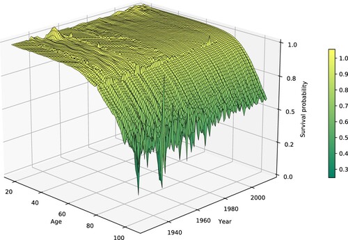
In the computational examples below, we employ the multivariate stochastic model presented in Maffra et al. (2021), which accounts for the statistical connections mentioned above and describes the main macroeconomic, financial and longevity risk factors affecting longevity-sensitive financial products. In particular, the model describes yearly returns on equities and bonds (money market, government, inflation-linked and corporate). The model also describes stochastic survival probabilities for cohorts of both genders with ages between 18 and 105. This high-dimensional space of random vectors is modeled using only six longevity risk factors. Each realization of these six stochastic processes can be used to construct yearly survival probability curves. Figure 1 plots historical survival rates for females from 1922 to 2016. A more detailed description of the longevity side of the model can be found in Aro and Pennanen (2011).

Figure 1. Yearly survival rates for females in the UK. Data is taken from the Human Mortality Database (Human Mortality Database, n.d.).

The stochastic model of Maffra et al. (2021) describes the evolution of the relevant risk factors by a linear stochastic difference equation (a.k.a. vector autoregression) of the form $\mathrm{\Delta }{\xi }_t=A{\xi }_{t-1}+a_t+{ϵ}_t,$where ${\xi }_t$ is a vector of transformed risk factors, $A\in {\mathbb{R}}^{d\times d}$ and $a_t\in {\mathbb{R}}^d$ are parameters and ${ϵ}_t$ are i.i.d. random innovations. The vector of transformed risk factors is defined as ${\xi }_t={[I_t,G_t,E_t,S_t,Y_t^s,Y_t^l,C_t,{\hat{I}}_t,v_t^{1,m},v_t^{2,m},v_t^{3,m},v_t^{1,f},v_t^{2,f},v_t^{3,f}]}^T,$with the components given in Table 1.

Table 1. Transformations of the economic risk factors.

Transformed risk factor	Description	Parameters
$I=\mathrm{\Delta ln}\left(\mathrm{CPI}\right)$	CPI log-growth (inflation)	–
$G=\mathrm{\Delta ln}\left(\frac{\mathrm{GDP}}{\mathrm{CPI}}\right)$	Real GDP log-growth	–
$E=\ln \left(\frac{\mathrm{AWE}}{\mathrm{CPI}}\right)$	Log real AWE	–
$S=\ln \left(\mathrm{StockIndex}\right)$	Log stock index	–
$Y^s=\ln \left(\frac{{\mathrm{YTM}}^s}{\frac{{\mathrm{CPI}}_t}{{\mathrm{CPI}}_{t-1}}}+\mu \right)$	Short-term bonds real YTM	$\mu =0.05$
$Y^l=\ln \left(\frac{{\mathrm{YTM}}^l}{\frac{{\mathrm{CPI}}_t}{{\mathrm{CPI}}_{t-1}}}+\mu \right)$	Long-term bonds real YTM	$\mu =0.05$
$C=\ln \left({\mathrm{YTM}}^{\mathrm{corp}}-{\mathrm{YTM}}^l+\mu \right)$	Log credit spread	$\mu =0.01$
$\hat{I}=\mathrm{LTIE}-I$	Inflation expectation spread	–
$v^{i,m}$, $v^{i,f}$	Mortality risk factors, i = 1, 2, 3	–

Notes: The risk factors include Consumer Price Index (CPI), Gross Domestic Product (GDP), Average Weekly Earnings (AWE), Long-term Inflation Expectations (LTIE), Yield-to-maturity for corporate, short and long-term bonds ($\mathrm{YT}{M}^{\mathrm{corp}}$, $\mathrm{YT}{M}^s$ and $\mathrm{YT}{M}^l$).

The time-dependent vectors $a_t$ allow for the calibration of the model to the user's views and forecasts; see Maffra et al. (2021, Section 4.2). In this study, we calibrate the model to the long-term median values given in Table 2. Except for the stock returns, the values are based on the ‘Long-term economic determinants’ published by the Office for Budget Responsibility (OBR) in Office for Budget Responsibility (2021) as part of a report on its outlook for the UK economy in the coming years. The median value for the stock index growth was chosen somewhat arbitrarily. The value of $6\mathrm{\%}$ for the median corresponds to a slightly higher value of roughly $7\mathrm{\%}$ for the mean. Assuming $2\mathrm{\%}$ average inflation, this would give about $5\mathrm{\%}$ real return which is in line with the long-term historical averages; see e.g. Dimson et al. (2023). In addition to the long-term views in Table 2, we specify the future median values of the money market rates according to the forward rates extracted from the ask prices of the zero-coupon bonds. Denoting the ask-price of the zero coupon bond with maturity t by $P_t$, the forward rate $F_t$ over $[t,t+1]$ is defined by $\frac{P_{t+1}}{P_t}=e^{F_t}⟺F_t=\mathrm{\Delta ln}{P}_{t+1}.$Market quotes for zero-coupon bonds and corresponding forward rates are illustrated in Figure 2. Of course, if one has different views concerning the future money market rates, one can use them instead of the forward rates. The forward rates can be thought of as market-neutral views that seem appropriate when no extra information is available.

Figure 2. The plot on the left shows the bid- and ask-prices observed for a set of gilt coupon strips on 08/Apr/2021. The corresponding forward rates, used to calibrate the median values of the money market rates are shown on the right.

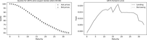
Table 2. Long-term views used in the stochastic modeling of the risk factors.

Long-term median views
Year	2070-71
Nominal GDP growth	3.9%
CPI inflation	2.0%
Average earnings growth	3.8%
Money market rates	4.1%
Gilt rates	4.1%
Stock index growth	6.0%

Notes: Except for the stock returns, the values are based on the ‘Long-term economic determinants’ published by the Office for Budget Responsibility (OBR) in Office for Budget Responsibility (2020). The median value for the growth of the stock index was chosen somewhat arbitrarily by the authors. It can be easily adjusted to match a user's views.

The money market is described by a single rate r so to describe the illiquidity of lending and borrowing, we add a margin on both sides so that the lending rate is $r_t^l=r_t-\delta$ and the borrowing rate $r_t^l=r_t+\delta$. Varying the illiquidity parameter δ will allow us to control the activity of the money market trading and control the time-matching of the liability cashflows; see Sections 5.2 and 5.3 below.

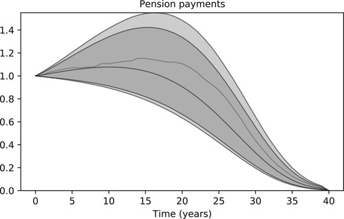
Simulated scenarios of the risk factors relevant to the (CDI) problem are illustrated in Figure 3. The same risk factors are used in the simulation of the pension liabilities illustrated in Figure 4. The numbers correspond to a cohort of 1000 females 65 years of age and an initial pension benefit of 1 GBP.

Figure 3. Historical and simulated values for the risk factors used in the computation of CDI portfolios. The 95% and 99% confidence bands obtained from a set of 100k simulated scenarios are illustrated in each plot along with a single simulated scenario. The rightmost risk factors correspond to longevity scenarios for females in the UK. Each realization of the three longevity risk factors reconstructs a survival probability surface such as the one illustrated in Figure 1.

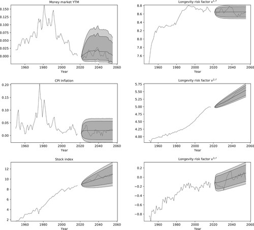
Figure 4. Pension payments to a cohort of 1000 65 year-old females that receive an initial benefit of 1 GBP. The 95% and 99% confidence bands are plotted along with a single scenario. Benefits are adjusted yearly, following the rules of the University Superannuation Scheme.

5. Computational results

5.1. Accuracy of the numerical approximations

When using a small sample size N in the approximation (CDId) of (CDI), one expects the optimal solution of (CDId) to violate the risk constraint in the original problem (CDI) where the risk measure is defined in terms of the original probability measure P. We perform a simple numerical experiment to analyze the approximation errors. For a given sample size N, we solve the optimization problem 50 times using independent random samples. For each of the 50 instances, we find the optimal portfolio, record the optimum value of (CDId), and numerically evaluate the risk measure corresponding to the optimized portfolio with an independent sample of $2^{18}=262,144$ scenarios. The out-of-sample evaluation is computed by rolling the money market position over time along every scenario using the budget constraint in (CDId).

We repeat the experiment with increasing sample sizes N (powers of 2) in order to study how the sample size affects the accuracy. The results are summarized in Table 3. As expected, the numerically optimized portfolios are infeasible in the sense that the out-of-sample evaluation of the risk measure is slightly positive. The out-of-sample values of the risk measure approach zero when the sample size increases. Similarly, the in-sample optimum values increase with N as more scenarios are added in the risk measure constraint of (CDId). With 32,768 scenarios, the numbers seem to have stabilized and the value of the risk measure seems acceptable given that it has units in cash and its value is about 10,000th of the initial wealth.

Table 3. Convergence of numerical approximations.

	Valuation (in-sample)		Risk measure (out-of-sample)		Computation time
N	Mean	SD	Mean	SD	Mean
1024	28.0708	0.1824	8.00e−04	5.41e−04	8.84
2048	28.1485	0.1016	4.99e−04	2.12e−04	20.27
4096	28.2406	0.0774	4.15e−04	2.47e−04	58.99
8192	28.2429	0.0494	3.83e−04	2.18e−04	180.38
16,384	28.2767	0.0338	3.43e−04	2.69e−04	463.09
32,768	28.2797	0.0352	2.96e−04	1.02e−04	819.64

Notes: For each sample size N, we generate a Monte Carlo approximation (CDId) 50 times and compute the corresponding optimal liability valuation. The average computational time is given in the rightmost column. The Valuation panel reports the mean and standard deviation (SD) of the valuations over the 50 samples. For each optimized hedge, we compute the value of the risk measure by using an independent sample of $2^{18}=\mathrm{262,144}$ scenarios. The Risk measure panel reports the mean and standard deviation (SD) of the obtained risk measure values. One out-of-sample computation took 0.60 seconds on average.

The last column of Table 3 gives the average time it takes to solve one instance of the optimization problem on an AMD Ryzen Threadripper 1950x desktop with 128 GB of RAM. The out-of-sample simulations were implemented using PyCUDA (Klöckner et al., 2012) and CUDA (NVIDIA Corporation, 2021), which reduced the computation times significantly. One out-of-sample computation over $2^{18}=\mathrm{262,144}$ scenarios took 0.60 seconds on average. The numerical results presented in Sections 5.3 and 5.4 were obtained with 32,768 scenarios in the optimization of the buy-and-hold portfolios in ?? and $2^{18}=\mathrm{262,144}$ out-of-sample scenarios in the analysis of the optimized portfolios.

5.2. CDI based on expectations

We start the numerical analysis of problem (CDI) by considering a completely deterministic model where all cashflows and investment returns are assumed known at time t = 0. We will assume that all risk factors follow their median values. This corresponds to current industry practices where CDI analysis is often done against a single scenario. Deterministic models are commonly used also in actuarial liability valuations which are based on discounting a single forecast of the future payments using deterministic discount factors. Despite being overly simplistic, the deterministic model allows us to illustrate some important features of problem (CDI).

In the first instance, we only use zero-coupon bonds as the hedging instruments. In the deterministic setting, the liability cashflows c can then be perfectly matched by buying $c_t$ units of the zero-coupon bond with maturity t. We confirm this numerically by solving problem (CDI) with a single scenario that follows the median forecast. The top-left plot in Figure 5 shows the yearly pension payments together with the cashflows of the hedging portfolio. Pension payments are illustrated with the solid line and the portfolio payouts by the vertical bars positioned at payment dates. The money market position over time (lending/borrowing) is represented by the dotted line. It should be noted that the optimal strategy involves zero trading in the money market. This is because the money market yields were calibrated to the quotes of the zero-coupon bonds as described in Section 4.3 so there is no incentive to invest in the money market. Moreover, the strictly positive spread between the lending and borrowing rates makes zero-coupon bonds a better investment than the money market. In this example, the margin between the lending and borrowing rates is $\delta =0.01$ basis points (BPS).

Figure 5. Illustration of the optimal portfolios in the deterministic model described in Section 5.2. The median annual pension payments are depicted by the solid black line while the cashflows of hedging portfolios are illustrated by the vertical bars. The money market position is given by the dashed line. The highly concentrated hedging portfolios in the top row correspond to an interest rate spread (margin) of $\delta =0.01$ basis points. When only zero-coupon bonds are considered, one obtains perfect cashflow matching already with $\delta =0.01$ but when including more instruments (the second and the third column) a much higher spread is required to incentivize perfect matching.

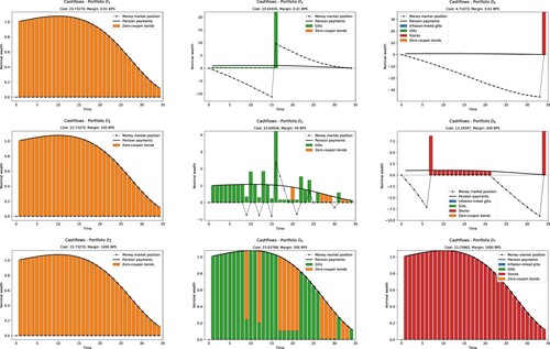
Next, maintaining the margin of $\delta =0.01$ BPS, we add coupon-paying bonds to the problem. In this setting, the optimal strategy invests the whole initial wealth into a single gilt and finances most of the liability payments by trading in the money market, as shown in the top-center plot of Figure 5. The poor diversification is explained by the lack of the risk-return trade-off in the deterministic model and the lower cost of gilts compared to zero-coupon bonds. While the risk-return trade-off can only be adequately studied in the stochastic case, the topic of Section 5.3, we can study the effect of changing the margin δ. When the interest rate spread is increased to $\delta =50$ BPS the trading activity in the money market decreases, and the optimal portfolio becomes more diversified as illustrated by the center plot of Figure 5. Perfect matching of the cashflows is obtained when we increase the margin to $\delta =200$ BPS. In this case, it is optimal to cover all payments by the statically held bonds and avoid borrowing from the money market.

We continue the experiment by adding stocks and inflation-linked bonds to the set of hedging instruments. The results should be interpreted with caution, however, as stocks and inflation-linked bonds are characterized by the uncertainty of their cashflows which cannot be described by a deterministic model. In the deterministic case, one cannot see the risks of stock investments nor the hedging properties of inflation-linked bonds. Essentially, the lack of risk in the deterministic model makes stocks seem underpriced while inflation-linked bonds seem overpriced. Nevertheless, we proceed with the experiment as this seems to be a common practice (more or less quantitatively) among investment advisors. The optimal hedging strategies are illustrated in the right column of Figure 5.

With an interest rate spread of $\delta =0.01$ BPS, the stock investments dominate in the deterministic model as it cannot account for the downside risk (top-right plot). The high median return makes stocks seem like the superior investment. Without uncertainty and with a low spread, the optimal portfolio invests everything in stocks which are liquidated at the end of the last period. All intermediate pension payments are financed by borrowing from the money market. When we increase the borrowing margin to $\delta =500$ BPS, the diversification is increased to reduce borrowing from the money market (middle-right plot). To perfectly match the cashflows, we have to increase the margin to $\delta =1000$ BPS. In this extreme case, borrowing costs become prohibitive so that the annual pension payments are covered by yearly liquidation of the equity investments (bottom-right plot).

This simple experiment illustrates how the illiquidity of the money market drives the temporal matching of the cashflows. With better matching comes an increase in hedging costs. Costs decrease, however, with additional hedging instruments. From an optimization perspective, it is clear that the inclusion of new instruments can only improve optimal solutions.

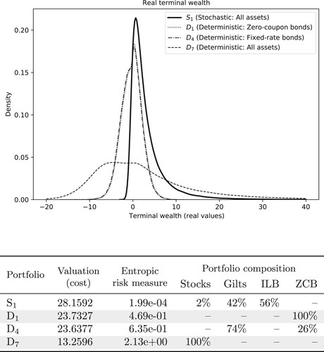
We end this section by analyzing the performance of the deterministically optimized portfolios in the stochastic model. To this end, we use the model described in Section 4.3 to simulate $2^{18}=\mathrm{262,144}$ scenarios for the pension payments and asset returns. For a given portfolio, the terminal fund wealth is easily computed by following the budget constraints in (CDId). Figure 6 gives kernel density plots for the terminal wealth distributions of each deterministically optimized portfolio. Portfolios that provide perfect cashflow matching in a deterministic model can be dangerously risky in a stochastic investment environment. The table in Figure 6 reports the hedging costs together with the entropic risk measure on the net terminal wealth. While the deterministically optimized hedging portfolios $D_1$, $D_4$ and $D_7$ come with a low cost, they provide a poor hedge in the uncertain world.

Figure 6. Comparison of the deterministic and stochastic approaches. The figure at the top illustrates the terminal wealth distributions obtained with deterministic and stochastically optimized portfolios. The deterministically optimized portfolios $D_1$, $D_4$ and $D_7$ present a high probability for negative outcomes. The probability is significantly reduced in the stochastically optimized portfolios. Note that portfolios $D_1$ and $D_4$ consist of fixed-rate bonds whose payouts match the median of liability payouts exactly. Accordingly, they result in identical terminal wealth distributions. The table presents the valuations and summarizes the portfolio compositions for the portfolios. The stochastically optimized portfolio $S_1$ is the most diversified and provides the best hedge against the liability cashflows in the face of uncertainty. This naturally comes at a cost reflected in the higher liability valuation.

5.3. CDI under uncertainty

We now move to the fully stochastic version of (CDI), where the cashflows of both the liabilities and the hedging instruments are random. This will allow us to quantify the risks and hedging potential of assets with cashflow uncertainties. Increasing the risk aversion will favor assets whose payouts better hedge against the pension liabilities. In the numerical experiments below, we find significant allocations in inflation-linked bonds that were not included in the deterministically optimized portfolios. A lower risk aversion, on the other hand, will favor assets with higher average payouts even if they are uncorrelated with the liability payments.

Our first results, with margin $\delta =100$ BPS and risk aversion $\rho =5$, are illustrated in Figure 7. In the stochastic case, we cannot present the results using the simple cashflow plots used in the deterministic case in Section 5.2. Instead, we create six different plots to illustrate the portfolios and their hedging properties in the stochastic case. In the top-left corner of the figure, we have a wealth allocation plot (not to be confused with the cashflow plots of Section 5.2) where the vertical bars at time t represent the aggregated amount of capital invested in hedging instruments maturing at that time. In this particular example, we have an optimal portfolio $S_1$ that invests, approximately, 1k GBP in gilts maturing at times $t=1,\dots ,7,13,14$; over 4k GBP in inflation-linked gilts maturing at times t = 10, 16, 20 and other smaller positions after t = 20. The optimal portfolio also holds a position of approximately 0.5k GBP in equities that is only liquidated at the final period.

Figure 7. Optimal hedging strategy $S_1$ obtained with risk aversion $\rho =5$ and margin $\delta =100$ BPS. The rightmost plots contain median values and 95% and 99% confidence bands. The leftmost plots illustrate the portfolio allocation and the terminal wealth; see the beginning of Section 5.3 for detailed descriptions of the subplots. The results are discussed in more detail in Sections 5.3.1 and 5.3.2.

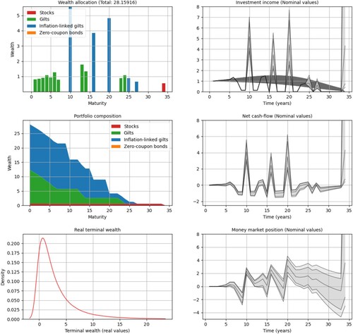
On the middle-left plot of Figure 7, we have a portfolio composition plot, in which stacked bands are used to illustrate the amount of capital invested in each asset class over time. In such plots, a drop occurs in one of the bands when one of the hedging instruments matures. Flat regions indicate positions being held fixed. Referring to the wealth allocation plot in the figure, for example, one can see a drop associated with the inflation-linked gilt maturing at time t = 10. One can also see the flat region corresponding to the position in stocks. It spans the entire simulation period, as the equities are liquidated only at the end.

In the top-right corner of Figure 7, we have an investment income plot, which illustrates the aggregated cashflows produced by the hedging strategy. The figures plot median values and 95% and 99% quantile bands of yearly cashflows. Deterministic cashflows, such as the ones from gilts and gilt strips, are represented as solid line segments. In this example, the optimal allocation has gilt positions maturing at times $t=1,\dots ,7$. The three spikes times at times $t=10,16$ and 20 correspond to the large positions in inflation-linked bonds. The cashflows corresponding to the position in stocks are only found when they are liquidated at time t = 34. The width of the confidence bands show how uncertain stock returns can be after a few decades. Pension payments are illustrated in the plot as the dark shape in the background; see Figure 4 for a comparison.

The three remaining plots in Figure 7 illustrate the development of the net cashflows and the money market position as well as the distribution of the terminal wealth. Again, we give the median values and the 95% and 99% quantile bands. The net cashflows are obtained simply by taking the difference of the investment income and the pension outflow so a surplus increases the money market position and vice-versa. The net cashflow is rolled over time through the money market account. Thus, the terminal wealth is simply the terminal position in the money market account.

The strategy illustrated in Figure 7 relies primarily on gilts to cover pension payments over the first 7 years. The strategy then resorts to borrowing from the money market, as the income from other investments is low in the next two years. The deficit in the money market position is then covered by the inflation-linked bond maturing at time t = 10. This creates a surplus of cash which is then invested in the money market. Around t = 15, we find quantile bands that span both negative and positive positions in the money market position, indicating a good chance of covering payments without resorting to borrowing from the money market. Most of the deficits are then covered in the following year by the inflation-linked bond position maturing at time t = 16. Income from gilts and an inflation-linked bond then create enough surplus to cover pension liabilities in the majority of cases until the time t = 30. Notice that the median value of the money market position becomes negative after that time. Finally, the position in equities is liquidated at time t = 34.

Inspecting the terminal wealth plot for $S_1$, in Figure 7, we notice a distribution of outcomes that is skewed toward positive values. We compare this distribution to those of the perfectly matching portfolios obtained with the deterministic model ($D_1$, $D_4$ and $D_7$) in Figure 6. Clearly, the portfolio $S_1$ provides better hedging to the pension liabilities, as the other portfolios present distributions that are approximately symmetric. The table in Figure 6 compares the different hedging strategies by their costs (liability valuations) and the risks as measured by the entropic risk measure. While the deterministically optimized portfolios are cheaper, they have a much higher level of risk than strategy $S_1$ obtained with stochastic optimization.

5.3.1. Effect of the lending and borrowing margin

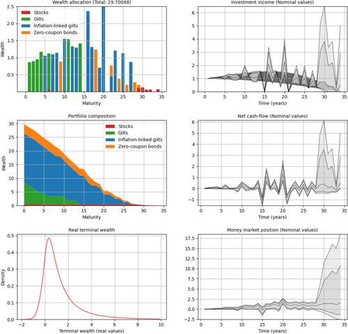
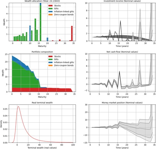
We will next illustrate the effect of the interest rate spread in the stochastic setup. Still with risk aversion $\rho =5$, we first increase the margin to $\delta =1000$ BPS. Then, we lower it to $\delta =0$ BPS reoptimizing in each case. In the first case, with the increased margin, we notice more diversification in the optimal portfolio $S_2$, illustrated in the wealth allocation plot of Figure 8. We also find an improved matching of cashflows in the investment income plot. Inspecting the money market position we see that, with an increased margin, the optimal strategy tends to avoid borrowing from the money market. Significant borrowing from the money market only occurs at the times t = 15 and t = 27. After the latter, the optimal portfolio is concentrated in stock investments, which explains the wide quantile bands at the end of the money market position and of the investment income plots. It is interesting to notice that the optimal portfolio $S_2$ now includes zero-coupon bonds. With higher money market costs, zero-coupon bonds provide a cheaper alternative for extra liquidity. The distribution of the terminal wealth still has a positive skew but it is now less risky than the portfolio $S_1$, illustrated in Figure 7. With the improved matching of cashflows and lower risk, we also observe an increase in cost for $S_2$.

Figure 8. Optimal hedging strategy $S_2$ with risk aversion $\rho =5$ and margin $\delta =1000$ BPS. The rightmost plots contain median values and 95% and 99% confidence bands. The leftmost plots illustrate the terminal wealth; see the beginning of Section 5.3 for detailed descriptions of the subplots. The results are discussed in more detail in Sections 5.3.1 and 5.3.2.

The case $S_3$ with zero margin is illustrated in Figure 9. As expected, we now see more activity in the money market and a reduced hedging cost, but also poorer matching of the cashflows over time and a less diversified portfolio. All the results obtained in this section are summarized in Table 4.

Figure 9. Optimal hedging strategy $S_3$ with risk aversion $\rho =5$ and margin $\delta =0$ BPS. The rightmost plots contain median values and 95% and 99% confidence bands. The leftmost plots illustrate the terminal wealth; see the beginning of Section 5.3 for detailed descriptions of the subplots. The results are discussed in more detail in Sections 5.3.1 and 5.3.2.

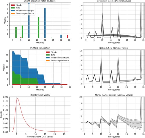
Table 4. Summary of results for the stochastically optimized hedging strategies.

				Portfolio composition
Portfolio	Margin	Risk aversion	Valuation (cost)	Stocks	Gilts	ILBs	ZCBs
S1	100	5	28.1592	2%	42%	56%	–
S2	1000	5	29.7009	2%	27%	60%	11%
S3	0	5	27.8031	3%	38%	59%	–
S4	100	1	24.1384	11%	76%	13%	–
S5	100	10	29.0350	1%	37%	61%	2%

Notes: $S_4$ has lower risk aversion, higher allocation in stocks and higher cost. $S_2$ has more diversification (uses all asset classes) and has the higher cost and better cashflow matching. As the risk aversion increases, we can see a higher cost as well ($S_1$, $S_3$ and $S_5$, with little change in the diversification).

Looking at the portfolio composition with fixed risk aversion and varying margin, we find that reduction of liquidity leads to increased allocation of zero-coupon and inflation-linked bonds and a reduction in gilts and equities. This is in line with the findings of Ang et al. (2014) who investigated the effects of liquidity risk on optimal portfolio composition. Their liquidity risk model was quite different from ours but they found a similar shift from riskier assets to safer ones when the liquidity risk is increased.

5.3.2. Effect of the risk aversion

We now fix the margin at $\delta =100$ BPS and analyze changes the effects of the risk aversion ρ. First, we lower the risk aversion from $\rho =5$ to $\rho =1$ and then increase it to $\rho =10$, reoptimizing after each change. With the lower risk aversion, illustrated in Figure 10, we notice that the optimal portfolio $S_4$ has a reduced allocation in inflation-linked bonds and an increase in stocks and gilts. Gilts now account for 76% of the invested capital. The wealth allocation plot shows that the hedging strategy expects to capitalize on the long-term returns of the stocks, as those are held until the end. The strategy also builds a surplus of capital in the early years, until t = 16. By increasing the allocation in stocks and trading in the money market, $S_4$ obtains the smallest cost among the portfolios in this section; see Table 4 (Figure 10).

Figure 10. Optimal hedging strategy $S_4$ with risk aversion $\rho =1$ and margin $\delta =100$ BPS. The rightmost plots contain median values and 95% and 99% confidence bands. The leftmost plots illustrate the terminal wealth; see the beginning of Section 5.3 for detailed descriptions of the subplots. The results are discussed in more detail in Sections 5.3.1 and 5.3.2.

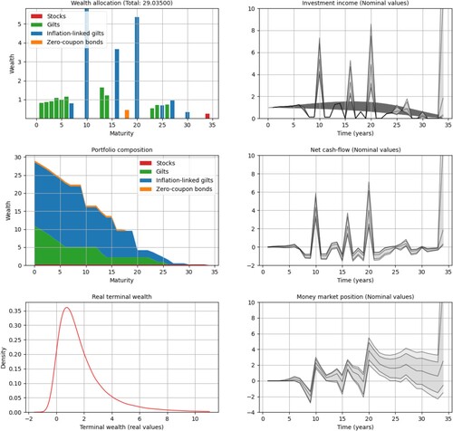
Increasing the risk aversion to $\rho =10$, we find a portfolio $S_5$ (illustrated in Figure 11) which has shifted capital from equities and gilts to inflation-linked bonds. The hedging cost has increased by 20%, and we find more diversification and less trading in the money market. Comparing $S_5$ to the original portfolio $S_1$, we see a mere 3% increase in the hedging cost with an increase of 5% in the capital allocated to inflation-linked bonds.

Figure 11. Optimal hedging strategy $S_5$ with risk aversion $\rho =10$ and margin $\delta =100$ BPS. The rightmost plots contain median values and 95% and 99% confidence bands. The leftmost plots illustrate the terminal wealth; see the beginning of Section 5.3 for detailed descriptions of the subplots. The results are discussed in more detail in Sections 5.3.1 and 5.3.2.

5.4. Liability valuations

This section takes a closer look at the liability valuations as a function of the risk aversion ρ and the lending and borrowing margin δ. To that end, we find optimal strategies and valuations with the risk aversions $\rho =0,1,\dots ,10$ and margins $\delta =0,100,\dots ,1000$. The resulting valuations are illustrated in Figure 12 in the form of a surface plot. As expected, valuations increase when either the interest rate margin or the risk aversion increases. Interestingly, the valuation seems to stabilize fairly quickly when the two parameters are increased and it seems to converge to around 30 k GBP.

Figure 12. Liability valuation as a function of the risk aversion ρ and the interest rate spread (margin) δ. The liabilities increase when either the margin or the risk aversion increases. When the risk aversion increases, the valuations stabilize rather quickly to around 27k to 30k GBP. The composition of the optimal portfolios and their corresponding terminal wealth distributions are illustrated in Figures 13 and 14.

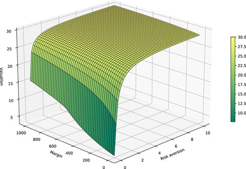
Figure 13. Portfolio allocations for different values of the risk aversion ρ and the interest rate spread (margin) δ. When the risk aversion increases, the allocations stabilize fairly quickly in accordance with the liability valuations in Figure 12

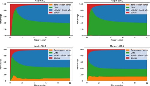
Figure 14. Terminal wealth distribution with varying risk aversion and interest rate spread. As expected, the dispersion of the terminal wealth and the risk of negative outcomes decrease as the risk aversion increases. The same happens when the margin is increased, as hedging strategies optimized with a higher margin provide better cashflow matching thus reducing the reinvestment risk.

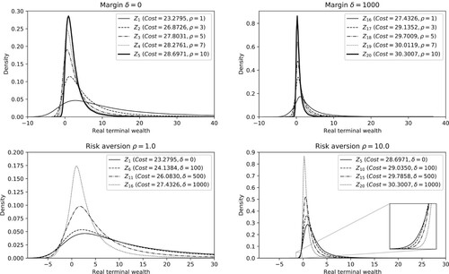
Figure 13 illustrates the composition of the optimal hedging strategies for different values of the margin and the risk aversion. Each plot in the figure represents the optimal allocations as functions of the risk aversion for a given margin. For risk aversion close to zero, stocks dominate the allocations but, as soon as the risk aversion ρ is increased, the stock allocations decrease sharply. When the risk aversion approaches 10, the allocations seem to stabilize with a small but nonzero investment in stocks. Gilts are added to the portfolios when the positions in stocks decrease. When the risk aversion is increased further, inflation-linked bonds begin to dominate. It seems that with low risk aversion, the hedging potential of the inflation-linked bonds is not worth the higher price they come with. When the risk aversion is increased, the proportion of inflation-linked bonds increases sharply and they eventually become the dominating asset class. Overall, the optimal asset proportions seem relatively stable for higher values of risk aversion.

Under liquid market conditions, zero-coupon bonds are absent in optimal allocations but, when the interest rate margin increases, they find their way into the portfolio (bottom plots in Figure 13). This is because zero-coupon bonds allow for precise control of the timing of the payments. When the timing is not an issue, coupon-paying gilts are preferred as they tend to provide higher yields.

The plots in Figure 14 show the distributions of real terminal wealth for different values of the interest rate margin and the risk aversion. As expected, the dispersion of the terminal wealth and the risk of negative outcomes decrease as the risk aversion increases. Interestingly, the same happens when the margin is increased. This phenomenon is easily seen in the bottom row of Figure 14 which superimposes the distributions for fixed risk aversions. Hedging strategies optimized with a higher margin provide better cashflow matching which reduces the reinvestment risk.

6. Conclusions

This paper presented a computationally tractable optimization model for cashflow-driven investment in the face of uncertainty over future liability payments and asset payouts. The model constructs optimal portfolios from hundreds of publically quoted hedging instruments within minutes on a regular PC. This makes the model a useful tool for analyzing and optimizing CDI strategies and for inspecting the effects of various modeling assumptions.

Besides optimal hedging strategies, the model finds the least cost of hedging which provides a market-consistent liability valuation based on the available quotes of hedging instruments and the liquidity factors as well as the views and risk preferences of the investor/regulator. Unlike traditional actuarial valuations, such hedging-based valuations are consistent with the principles of financial economics as well as general accounting standards in describing the cost of hedging a given liability in the face of uncertainty.

The approach was illustrated by pricing and hedging defined benefit pension liabilities which depend on uncertain longevity developments and the consumer price index. We found, in particular, that the common practice of cashflow matching is largely motivated by liquidity risk in the money market. When liquidity is reduced, the optimal hedging strategy aims to match the liability cashflows over time. In liquid markets, on the other hand, the timing of the payments is less of a concern as one can more easily finance payments by money market operations.

The stochastic model also provides a good illustration of the dangers of CDI strategies based on deterministic models. In a deterministic model, it is easy to construct hedging strategies that seem to provide good cashflow matching over the life of the liabilities but those strategies turn out to have a significantly higher shortfall risk than the hedging strategies optimized for the stochastic future.

The presented models and computational techniques are not limited to pensions and the hedging instruments employed in the computational examples in this paper. The same approach could be taken in pricing and hedging of e.g. corporate debt, index-liked bonds or any other liability described in terms of contractual future payments. The payouts of corporate debt could be modeled e.g. by incorporating default intensity factors in the underlying stochastic model of the risk factors. Corporate bonds will be an important addition to the space of hedging instruments when the models presented in this paper are implemented in practice.

Disclosure statement

No potential conflict of interest was reported by the author(s).

Additional information

Funding

This work was supported by Pensions Policy Institute.

References

- Agrawal, A., Verschueren, R., Diamond, S., & Boyd, S. (2018). A rewriting system for convex optimization problems. Journal of Control and Decision, 5(1), 42–60. https://doi.org/10.1080/23307706.2017.1397554
- Ang, A., Papanikolaou, D., & Westerfield, M. M (2014). Portfolio choice with illiquid assets. Management Science, 60(11), 2737–2761. https://doi.org/10.1287/mnsc.2014.1986
- Aro, H., & Pennanen, T. (2011). A user-friendly approach to stochastic mortality modelling. European Actuarial Journal, 1(2), 151–167. https://doi.org/10.1007/s13385-011-0030-4
- Aro, H., & Pennanen, T. (2014). Stochastic modelling of mortality and financial markets. Scandinavian Actuarial Journal, 2014(6), 483–509. https://doi.org/10.1080/03461238.2012.724442
- Artzner, Ph., Delbaen, F., Eber, J.-M., & Heath, D. (1999). Coherent measures of risk. Mathematical Finance, 9(3), 203–228. https://doi.org/10.1111/mafi.1999.9.issue-3
- Ben-Tal, A., & Teboulle, M. (2007). An old-new concept of convex risk measures: The optimized certainty equivalent. Mathematical Finance, 17(3), 449–476. https://doi.org/10.1111/mafi.2007.17.issue-3
- Best, M. J., & Hlouskova, J. (2005). An algorithm for portfolio optimization with transaction costs. Management Science, 51(11), 1676–1688. https://doi.org/10.1287/mnsc.1050.0418
- Boyles, G. V., Secrest, T. W., & Burney, R. B. (2005). The pricing of bonds between coupon payments: From theory to market practice. Journal of Economics and Finance Education, 4(2), 61.
- Diamond, S., & Boyd, S. (2016). CVXPY: A Python-embedded modeling language for convex optimization. Journal of Machine Learning Research, 17(83), 1–5.
- Dimson, E., Marsh, P., & Staunton, M. (2023). Credit Suisse global investment returns yearbook 2023 summary edition.
- Exley, J. (2017, September). Cashflow driven investment or clever distribution investing? Available at http://tiny.cc/9mmvtz.
- Föllmer, H., & Schied, A. (2016). Stochastic finance. De Gruyter Graduate. De Gruyter. An introduction in discrete time, Fourth revised and extended edition of [MR1925197].
- Geyer, A., & Ziemba, W. T. (2008). The innovest Austrian pension fund financial planning model InnoALM. Operations Research, 56(4), 797–810. https://doi.org/10.1287/opre.1080.0564
- Glasserman, P. (2013). Monte Carlo methods in financial engineering (Vol. 53). Springer Science & Business Media.
- Hamilton-Glover, M. (2018, February). Trends in the uk mortality experience [MPhil Dissertation]. King's College London.
- Heaven, K., Fazal, M., & White, A. (n.d.). Destination endgame. Available at http://tiny.cc/3lmvtz.
- Hilli, P., Koivu, M., & Pennanen, T. (2011). Cash-flow based valuation of pension liabilities. European Actuarial Journal, 1, 329–343. https://doi.org/10.1007/s13385-011-0023-3
- Human Mortality Database (n.d.). University of California, Berkeley (USA), and Max Planck Institute for Demographic Research (Germany). Human mortality database. Available at www.mortality.org.
- Insight Investment (n.d.). Cashflow driven investment (CDI). Available at http://tiny.cc/co0wtz.
- Institute and Faculty of Actuaries (2019, December). A holistic study into cash flow driven investment. Available at http://tiny.cc/jinvtz.
- Kazziha, S., Martel, R., & Burns, M. A. (2019, June). Cashflow driven investing: Does it make sense for uk db schemes? Available at http://tiny.cc/oinvtz.
- Klöckner, A., Pinto, N., Lee, Y., Catanzaro, B., Ivanov, P., & Fasih, A. (2012). PyCUDA and PyOpenCL: A scripting-based approach to GPU run-time code generation. Parallel Computing, 38(3), 157–174. https://doi.org/10.1016/j.parco.2011.09.001
- Maffra, S. A., Armstrong, J., & Pennanen, T. (2021). Stochastic modeling of assets and liabilities with mortality risk. Scandinavian Actuarial Journal 2021, 2021(8), 1–31.
- Mcinally, K. (2019, February). What is cashflow driven investment? Available at http://tiny.cc/hmmvtz.
- MOSEK ApS (2021). MOSEK Optimizer API for Python 9.2.46.
- Mulvey, J. M., Simsek, K. D., Zhang, Z., Fabozzi, F. J., & Pauling, W. R. (2008). Or practice–assisting defined-benefit pension plans. Operations Research, 56(5), 1066–1078. https://doi.org/10.1287/opre.1080.0526
- NVIDIA Corporation (2021). CUDA Toolkit Documentation. NVIDIA Corporation.
- Office for Budget Responsibility (2020, March). Long-term economic determinants. Available at https://obr.uk/efo/economic-and-fiscal-outlook-march-2020/.
- Office for Budget Responsibility (2021, March). Economic and fiscal outlook – March 2021. Available at http://tiny.cc/sdjytz.
- Pennanen, T. (2014). Optimal investment and contingent claim valuation in illiquid markets. Finance and Stochastics, 18(4), 733–754. https://doi.org/10.1007/s00780-014-0240-0
- Pensions and Lifetime Savings Association (2019, October). Cashflow driven investment made simple. Available at http://tiny.cc/linvtz.
- Rockafellar, R. T. (1974). Conjugate duality and optimization. Society for Industrial and Applied Mathematics.
- Sodhi, M. S. (2005). LP modeling for asset-liability management: A survey of choices and simplifications. Operations Research, 53(2), 181–196. https://doi.org/10.1287/opre.1040.0185
- United Kingdom Debt Management Office (2005, March). Formulae for calculating gilt prices from yields. Available at http://tiny.cc/ldsvtz.
- United Kingdom Debt Management Office (2012, June). Uk government securities: A guide to ‘Gilts’. Available at http://tiny.cc/ojpvtz.
- Uryasev, S., & Rockafellar, R. T. (2001). Conditional value-at-risk: Optimization approach. In Stochastic optimization: Algorithms and applications (Gainesville, FL, 2000): Vol. 54. Appl. Optim. (pp. 411–435). Kluwer Acad. Publ.
- USS (2018). Your guide to the universities superannuation scheme. Available at http://tiny.cc/fazvty.
- Van Rossum, G., & Drake, F. L. (2009). Python 3 reference manual. CreateSpace.
- Watson, W. T. (2019, April). Cashflow driven investment: Ultimate solution to the pensions problem, or just glorified liability-driven investment? Available at http://tiny.cc/olmvtz.