Money illusion in retirement savings with a minimum guarantee

Abstract

We investigate the impact of money illusion on the investment strategy and retirement outcomes of pre-retirees. Money illusion refers to the tendency of individuals to overlook the effects of inflation and focus on nominal rather than real terms. We solve and compare the optimal investment strategies for a pre-retiree who exhibits money illusion and aims to maximize the expected power utility of wealth at retirement, subject to a minimum guarantee constraint. While money illusion leads to welfare losses, implementing a minimum guarantee helps suppress these losses. However, guarantee constraints set under money illusion are ineffective in meeting inflation-adjusted constraints. Our findings emphasize the significant impact of money illusion on pre-retirees' investment strategy and retirement outcomes in the form of utility loss and the risk of falling short of the minimum guarantee.

Keywords:

• Money illusion
• inflation
• constrained optimization
• portfolio choice
• retirement outcomes

1. Introduction

Inflation eating away at the value of pension savings is a concern for many pre-retirees. If left unchecked, inflation can erode the purchasing power of retirement savings over a long period of time. A 2021 survey of American pre-retirees found that 66% were worried that the value of their savings and investments might not keep up with inflation (Greenwald Research, 2022, Table 4). A recent survey of savers from Australia, US, UK and Ireland in 2022 found that 65% of respondents say they wish for a consistent stream of income in retirement (State Street Global Advisors, 2022).

Yet reality shows us that these concerns, worries and desires are ignored in practice. Retirement goals in defined contribution pension plans are usually expressed in nominal terms as maximizing the absolute size of wealth at retirement. Over 90% of UK annuitants choose to buy a level life annuity despite expressing a preference for an inflation-indexed annuity before purchase (Finkelstein & Poterba, 2004). People do not naturally think in inflation terms – future inflation is, after all, an abstract, nebulous idea. It is not natural, when asked about your retirement savings goals, to allow for inflation. Instead, we think in today's money terms – not yesterday's or tomorrow's economic world. We adopt the term money illusion¹ to describe this behavioral bias towards thinking in nominal terms rather than in real terms (Shafir et al., 1997). In our work, we adapt the formulation in Basak and Yan (2010) and Miao and Xie (2013) that allows for a partial money illusion behavioral bias, which can be interpreted as a manifestation of underestimation of inflation risk. Empirically, a recent survey of financial professionals indicates that financial professionals around the world regard underestimating the impact of inflation as the number one mistake investors make in their retirement planning (Natixis Investment Managers, 2022).

Classical optimal control problems in pension savings first excluded inflation (Merton, 1969, 1971). However, many authors have since integrated inflation into these classical problems. For example, Menoncin (2002) derived the solution for an investor maximizing the expected exponential utility under inflation risk in a complete market. Brennan and Xia (2002), Battocchio and Menoncin (2004) and Zhang and Guo (2018) studied the investor's problem in an incomplete market without an inflation-linked bond. The former two showed that the inflation risk can instead be partially hedged via a cash-dominated portfolio with a high correlation with inflation and the cost imposed by unhedgeable inflation risk is surprisingly low. Notably, the majority of these works assume that the investors are rational and fully aware of inflation risk. It was only recently that Lioui and Tarelli (2023) and Wei and Yang (2023) began to study the pension savings problem by modeling money illusion as a failure to fully account for inflation risk by adopting the preference formulation as in Basak and Yan (2010) and Miao and Xie (2013).

Many optimal control problems include a minimum guarantee. The minimum guarantee, also known as the lower terminal wealth constraint, is a practical and attractive tool in planning for retirement Alles (2011). Several forms of the lower wealth constraint are studied, ranging from static minimum constraint(s) (Barucci et al., 2021; Ding & Marazzina, 2022; Korn, 2005; Kraft & Steffensen, 2013) to a minimum performance relative to a benchmark strategy (Boulier et al., 2001; Chen et al., 2017; Han & Hung, 2012; Teplá, 2001). However, the addition of a minimum guarantee inevitably complicates the investment strategy and introduces susceptibility to money illusion, especially for investors aiming for an inflation-indexed amount that maintains purchasing power over an extended investment horizon.

Inflation significantly impacts pre-retirees due to the long-term nature of retirement savings. However, many individuals are subject to behavioral biases that hinder their ability to fully account for inflation risk. Our research contributes to existing literature by investigating the impact of money illusion in the presence of a minimum guarantee. We assume an investor who derives utility from real wealth and requires an inflation-indexed annuity at retirement. This investor may be subject to money illusion during their savings phase, which impedes their ability to fully consider inflation risk in two aspects: (A) evaluating the utility of wealth and (B) setting the minimum guarantee constraint. Then, we solve investment problems for the investor who may suffer a varying extent of money illusions in these two aspects. Next, we compare the suboptimal investment strategies derived under money illusion and analyze their resultant retirement outcomes.

Our results demonstrate that the impacts of these two aspects of money illusion are largely isolated to the ‘unconstrained’ component or the hedging component of the overall investment strategy. Aspect A influences the unconstrained component, shaping the risk profile of the investment while incorporating the hedging mechanism required by the minimum guarantee. Contrary to the findings of Zhang (2012), we show that adopting an inflation-adjusted risk perception yields a different optimal strategy to the Merton strategy by having an additional inflation risk hedging component in the absence of a minimum guarantee. Under realistic parameters, we find that neglecting inflation risk reduces investor welfare by 19.5% for a medium risk averse investor without a minimum guarantee. Importantly, our results suggest that introducing a minimum guarantee can significantly suppress welfare loss, reducing the welfare loss to 7.6% for a medium risk averse investor. However, this comes with the susceptibility to aspect B of money illusion. If inflation risk is incorrectly specified when determining the minimum guarantee, the guarantee becomes ineffective, consequently exposing the investor to the risk of not fulfilling the inflation-indexed guarantee.

The paper is organized as follows: Section 2 presents the market model and the investor's preferences. In Section 3, we provide the solution to the investment problem with a minimum guarantee constraint under money illusion. Section 4 provides numerical illustrations and discussions on the optimal strategies, certainty equivalent loss, and the risk of not meeting the minimum guarantee when inflation risk is not fully accounted for. Section 5 concludes the paper.

2. Model setup

2.1. Description of the markets

In the classical lifecycle literature, the investor seeks to maximize the expected utility of their nominal wealth at retirement. In contrast, the investor seeks to maximize real wealth and not nominal wealth in our model. To do this, while keeping a nominal asset in the model, requires a model of inflation. We model inflation through a price index. The value of the price index is $P(t)$ at time $t\ge 0$, with dynamics (1) $\mathrm{d}P(t)=P(t){\mu }_P\mathrm{d}t+P(t){\sigma }_P\mathrm{d}{W}_1(t),P(0)=1\mathrm{a}.\mathrm{s}.,$(1) in which ${\mu }_P$ is the expected increase in the index, ${\sigma }_P>0$ is the constant volatility of the index and $W_1$ is a standard Brownian motion. Changes in the value of the price index represent inflation in our model. Note that the index is not an asset and is not traded in the market.

Following Karatzas and Shreve (1998), we assume that the investor trades d + 1 assets in a continuous-time market without transaction costs over a finite time horizon $[0,T]$ for T>0. We refer to T as the terminal time or retirement time. One of the traded assets is a nominal bond which increases at a constant rate, with dynamics $\mathrm{d}{S}_0(t)=S_0(t)r_{\mathrm{N}}\mathrm{d}t,S_0(0)=1\mathrm{a}.\mathrm{s}.,$for a constant real number $r_{\mathrm{N}}$ that represents the nominal annual risk-free interest rate.

When the investor seeks to maximize nominal wealth at retirement, the nominal bond is the risk-free asset. However, the risk perception of the nominal bond changes when the investor seeks to maximize the expected utility of their real wealth. The nominal bond becomes a risky asset, as it provides no protection against inflation. To enable the investor to hedge against the inflation risk, an index-linked bond (ILB), $S_1$, is introduced into the financial market (see e.g. Chen et al., 2023, 2017; Donnelly et al., 2022; Zhang & Ewald, 2010). For simplicity, we assume that the real return on the ILB is constant, at the annual rate $r_{\mathrm{R}}$, which yields a nominal rate of return of ${\mu }_1={\mu }_P+r_{\mathrm{R}}$. The dynamics of the price of the ILB are (2) $\mathrm{d}{S}_1(t)=S_1(t)(r_{\mathrm{R}}+{\mu }_P)\mathrm{d}t+S_1(t){\sigma }_P\mathrm{d}{W}_1(t),S_1(0)=S_{1,0}>0,\mathrm{a}.\mathrm{s}.$(2) It is seen by comparing the dynamics in (1(1) $\mathrm{d}P(t)=P(t){\mu }_P\mathrm{d}t+P(t){\sigma }_P\mathrm{d}{W}_1(t),P(0)=1\mathrm{a}.\mathrm{s}.,$(1) ) and (2(2) $\mathrm{d}{S}_1(t)=S_1(t)(r_{\mathrm{R}}+{\mu }_P)\mathrm{d}t+S_1(t){\sigma }_P\mathrm{d}{W}_1(t),S_1(0)=S_{1,0}>0,\mathrm{a}.\mathrm{s}.$(2) ), that the price of the ILB is perfectly correlated with the value of the price index since they are both driven by the same Brownian motion.

Note that the nominal return of the ILB is not known until the bond is redeemed at maturity or sold. This is because the value of the price index is a random process. However, the real return is known in our model². Our approach here is to fix the real return, and from the real return and the price index model above we can infer the price of ILB at any time.

The prices of the remaining traded risky assets $S_n$ for $n=1,\dots ,d$ follow the dynamics (3) $\mathrm{d}{S}_n(t)=S_n(t){\mu }_n\mathrm{d}t+\sum _{j=1}^n{S}_n(t){\sigma }_{\mathrm{nj}}\mathrm{d}{W}_j(t),S_n(0)=S_{n,0}>0,$(3) with a constant mean rate of return ${\mu }_n$ and volatilities coefficients ${\sigma }_{\mathrm{nj}}>0$ with $W_j$ for $j=1,\dots ,n$.

Define $\mu \mu =\left(\begin{array}{c}{\mu }_1\\ {\mu }_2\\ ⋮\\ {\mu }_d\end{array}\right),\sigma \sigma =\left(\begin{array}{cccc}{\sigma }_P& 0& \cdots & 0\\ {\sigma }_{21}& {\sigma }_{22}& \cdots & 0\\ ⋮& ⋮& & ⋮\\ {\sigma }_{d1}& {\sigma }_{d2}& \cdots & {\sigma }_{\mathrm{dd}}\end{array}\right),$in which it is assumed that $\sigma \sigma$ is non-singular. Within the considered market, we have the market price of risk $\theta \theta :=\sigma {\sigma }^{-1}(\mu \mu -r_{\mathrm{N}}11_d)$ where $11_d$ represent a d-column vector of ones. We assume that $\Vert \theta \theta \Vert >0$, where $\Vert .\Vert$ denotes the square norm of a vector in this paper.

For the technical conditions, the vector process $\mathbf{W}:=(W_1,\dots ,W_d{)}^{\mathrm{\prime }}$ is a d-dimensional Brownian motion under a real-world probability measure $\mathbb{P}$. The information ${\mathcal{F}}_t$ available to market investors at each time $t\in [0,T]$ is the natural filtration generated by $\mathbf{W}$, augmented by its $\mathbb{P}$-null sets. For a process η, we write $\eta \in {\mathcal{F}}^{\star }$ to indicate that it is ${\mathcal{F}}_t$-progressively measurable. The expectation operator under $\mathbb{P}$ is denoted $\mathbb{E}$.

2.2. Investor

We consider a pre-retiree investor who participates in the labor market and makes contributions to their savings (fund) before retirement time T. We assume that the investor contributes a fixed percentage, c $(0\le c\le 1)$ of labor income to the fund continuously before retirement time T. We further assume that the labor income of the investor is stochastic and follows (4) $\mathrm{d}Y(t)=Y(t){\mu }_Y\mathrm{d}t+Y(t)\sigma {\sigma }_Y^{\mathrm{\prime }}\mathrm{d}\mathbf{W}(t),Y(0)=1>0,\mathrm{a}.\mathrm{s}.$(4) where ${\mu }_Y$ is the deterministic appreciation rate³, and $\sigma {\sigma }_Y$ is the vector of volatility coefficients for the d-dimensional Brownian motion⁴.

The investor demands a minimum guarantee to secure a minimum level of wealth $G(T)$ in the retirement date T. This amount can be calculated as the amount of money required to secure the minimum inflation-indexed income required by the investor for their retirement which we specify further in Section 2.4.

The decisions made by the pre-retiree investor today (i.e. at time 0) with a fixed non-random initial wealth $x_0>0$ dependent on:

• an integer T>0 corresponding to their planned retirement date.

• a minimum retirement amount $G(T)$ representing the minimum amount of money the investor would like to have at retirement.

The value of the investor's fund at time t is represented by $X^{\pi \pi }(t)$. The superscript $\pi \pi$ refers to an investment strategy which is a vector process $\pi \pi =({\pi }_1\dots ,{\pi }_d{)}^{\mathrm{\prime }}\in {\mathcal{F}}^{\star }$ in which:

• ${\pi }_1(t)$ is the proportion of wealth invested in the ILB at time t, and

• ${\pi }_i(t)$ is the proportion of wealth invested in the i-th risky stock at time t for $i=2,\dots ,d$.

The remainder of the proportion of the investor's fund ${\pi }_0(t):=1-\sum _{n=1}^d{\pi }_n(t)=1-\pi {\pi }^{\mathrm{\prime }}11_d$is invested in the nominal bond.

The dynamics of the investor's fund value are (5) $\mathrm{d}{X}^{\pi \pi }(t)=(X^{\pi \pi }(t)r_{\mathrm{N}}+X^{\pi \pi }(t)\pi {\pi }^{\mathrm{\prime }}(t)\sigma \sigma \theta \theta )\mathrm{d}t+X^{\pi \pi }(t)\pi {\pi }^{\mathrm{\prime }}(t)\sigma \sigma \mathrm{d}\mathbf{W}(t)+\mathrm{cY}(t)\mathrm{d}t,$(5) with the initial condition that $X^{\pi \pi }(0):=x_0>0$, a.s. and $\mathrm{cY}(t)$ is the amount of money contributed to the investor's fund at time $t\in [0,T]$. Define $D(t)$ as the time-t-value of future contributions: (6) $D(t)=c{\mathbb{E}}_t[{\int }_t^{T}Y(s)\frac{H(s)}{H(t)}\mathrm{d}s].$(6) The properties of $D(t)$ are given in Proposition 2.1.

Proposition 2.1

(i)	The present value of the expected future contribution process is (7) $D(t)=\frac{c}{\delta }[e^{\delta (T-t)}-1]Y(t),$(7) where $\delta ={\mu }_Y-r_{\mathrm{N}}-\sigma {\sigma }_Y^{\mathrm{\prime }}\theta \theta$.
(ii)	The time-t-value of the expected future contribution satisfies the following dynamics (8) $D(t)=(r_{\mathrm{N}}+\sigma {\sigma }_Y^{\mathrm{\prime }}\theta \theta )D(t)\mathrm{d}t+\sigma {\sigma }_Y^{\mathrm{\prime }}D(t)\mathrm{d}\mathbf{W}(t)-\mathrm{cY}(t)\mathrm{d}t,$(8) with the initial condition that $D(0)=d_0$, a.s.

Proof.

See Appendix A.1

The set of admissible portfolios for the investor's initial wealth $x_0$ is defined to be $\begin{array}{rl}\mathcal{A}(x_0)& :=\{\phantom{{\int }_t^T}\pi \pi :\mathrm{\Omega }\times [0,T]\to {\mathbb{R}}^d|\phantom{{\int }_t^T}\pi \pi \in {\mathcal{F}}^{\star },X^{\pi \pi }(0)=x_0,\mathrm{a}.\mathrm{s}.\\ & \mathrm{and}{X}^{\pi \pi }(t)+c{\mathbb{E}}_t[{\int }_t^{T}Y(s)\frac{H(s)}{H(t)}\mathrm{d}s]\ge 0,\mathrm{\forall }t\in (0,T]\mathrm{a}.\mathrm{s}.\}.\end{array}$A portfolio $\pi \pi$ must satisfy the budget constraint that the initial wealth is sufficient to attain the retirement wealth that results from the following portfolio $\pi \pi$. Mathematically, we write the budget constraint as (9) $\mathbb{E}(H(T)X^{\pi \pi }(T))\le x_0+d_0.$(9) where (10) $\mathrm{d}H(t)=-H(t)r_{\mathrm{N}}\mathrm{d}t-H(t)\theta {\theta }^{\mathrm{\prime }}\mathrm{d}\mathbf{W}(t),H(0)=1\mathrm{a}.\mathrm{s}.$(10) For analytical trackability, we work with the budget constraint (9(9) $\mathbb{E}(H(T)X^{\pi \pi }(T))\le x_0+d_0.$(9) ). However, we note that the budget constraint (9(9) $\mathbb{E}(H(T)X^{\pi \pi }(T))\le x_0+d_0.$(9) ) may not be realistic since in practice it is not allowed for $X^{\pi \pi }(t)$ to be negative at any time t.

2.3. Preference

To set the investment strategy, the investor seeks to maximize the expected value of their real wealth at retirement subject to the minimum guarantee constraint. For mathematical simplicity, the utility function of the investor is assumed to be the power utility function⁵ $U(\tilde{X}(T))=\frac{\tilde{X}(T{)}^{1-\gamma }}{1-\gamma }$for a constant $\gamma >0$ and $\tilde{X}(T)=X(T)/P(T)>0$ is the investor's real wealth at retirement time T. Following Lioui and Tarelli (2023) and Wei and Yang (2023), we assume that the investor suffers from money illusion and is therefore biased towards making decisions in nominal terms rather than in real terms. When the investor is money-illusioned in utility evaluation (aspect A), we assume that the investor calculates their utility based on $X(T)/P(T{)}^{1-\alpha }$ instead of $\tilde{X}(T)$, so that (11) $U(X(T)/P(T{)}^{1-\alpha })=\frac{1}{1-\gamma }{(X(T)/P(T{)}^{1-\alpha })}^{1-\gamma }$(11) where α represents the degree of money illusion in evaluating the utility derived from wealth. The case in which $\alpha =0$ represents an investor who is free from aspect A illusions, consequently maximizing the expected utility based on real wealth only. In contrast, when $\alpha =1$, the investor suffers from complete money illusion in aspect A, perceiving purchasing power solely in nominal terms and thus maximizing the expected utility based on nominal wealth only. When $0<\alpha <1$, the investor exhibits partial money illusion, neglecting some inflation risk and using a mix of nominal and real wealth in the utility function. Therefore, $\alpha \in (0,1)$ can be interpreted as a manifestation of the investor's underestimation of inflation risk. The weight α reflects the relative significance placed on nominal wealth due to the presence of money illusion.

2.4. Minimum guaranteee constraint

The investor seeks a minimum guarantee of wealth level at retirement to be the price of an inflation-indexed income stream that pays an amount k continuously from the retirement date T to $$\begin{gathered} T^{{ \\ }^{\prime }} \end{gathered}$$ where $$\begin{gathered} T^{{ \\ }^{\prime }}>T \end{gathered}$$ denotes the time of death which we assume to be a constant⁶. Then, the value of the minimum guarantee of the investor at time T is $$\begin{gathered} G(T)={\mathbb{E}}_T[{\int }_T^{T^{{ \\ }^{\prime }}}\mathrm{kP}(s)\frac{H(s)}{H(T)}\mathrm{d}s]. \end{gathered}$$Having a minimum guarantee introduces an additional vulnerability towards money illusion where the investor may mistakenly target a static stream of income in retirement instead of an inflation-indexed stream of income (aspect B). Let β represent the degree of money illusion in provisioning for future inflation in setting up the minimum guarantee requirement. Then, an investor who suffers from money illusion sets their minimum guarantee as (12) $$\begin{gathered} G_{\beta }(T)={\mathbb{E}}_T[{\int }_T^{T^{{ \\ }^{\prime }}}\mathrm{kP}(s{)}^{1-\beta }\frac{H(s)}{H(T)}\mathrm{d}s]. \end{gathered}$$(12) When $\beta =0$, it represents an investor who accurately considers the impact of inflation when determining the minimum guarantee. In contrast, when $\beta =1$, the investor suffers from complete money illusion and fails to account for the changes in future purchasing power caused by inflation. As a result, they set a minimum guarantee to provide a constant rate of income k from T to $$\begin{gathered} T^{{ \\ }^{\prime }} \end{gathered}$$. For $0<\beta <1$, the investor demonstrates partial money illusion by partly overlooking inflation and incorporating partial inflation indexation into their desired income at retirement⁷. The weight $1-\beta$ quantifies the extent of inflation indexation utilized.

3. Optimization problem with a minimum guarantee

We consider the optimization problem in which the money-illusioned investor seeks to maximize the expected utility of their real wealth at retirement subject to a minimum guarantee that secures the value of an inflation-indexed annuity that continuously pays k from T to $$\begin{gathered} T^{{ \\ }^{\prime }} \end{gathered}$$. As discussed in Section 2.4, the inclusion of a minimum guarantee exposes the investor to an additional aspect of money illusion. Specifically, β captures the extent to which the investor fails to correctly consider inflation risk associated with their retirement income stream. Therefore, allowing for potential money illusion, the investment problem from which the investor devises their investment strategy is given by (13) $\begin{array}{rl}\underset{\pi \pi \in \mathcal{A}(x_0)}{sup}& \mathbb{E}\left[U(X^{\pi \pi }(T)/P(T{)}^{1-\alpha })\right]\\ \mathrm{subjectto}& X^{\pi \pi }(T)\ge G_{\beta }(T),\\ \mathrm{and}& \pi {\pi }^{\prime }\mathrm{satisfying}(4)\mathrm{and}(5),\end{array}$(13) Now, we give some properties of $G_{\beta }(t)$.

Proposition 3.1

(i)	The time-t-value of the guarantee with β-level of money illusion is (14) $$\begin{gathered} G_{\beta }(t)=\frac{k}{{\eta }_{\beta }}[e^{{\eta }_{\beta }(T^{{ \\ }^{\prime }}-t)}-e^{{\eta }_{\beta }(T-t)}]P(t{)}^{1-\beta }, \end{gathered}$$(14) where ${\eta }_{\beta }=(1-\beta ){\mu }_P-\frac{1}{2}\beta (1-\beta ){\sigma }_P^2-r_{\mathrm{N}}-(1-\beta )\sigma {\sigma }_P^{\mathrm{\prime }}\theta \theta$.
(ii)	The time-t-value of the guarantee satisfies the following dynamics (15) $\mathrm{d}{G}_{\beta }(t)=(r_{\mathrm{N}}+(1-\beta )\sigma {\sigma }_P^{\mathrm{\prime }}\theta \theta )G_{\beta }(t)\mathrm{d}t+(1-\beta )\sigma {\sigma }_P^{\mathrm{\prime }}{G}_{\beta }(t)\mathrm{d}\mathbf{W}(t),$(15) with the initial value $G_{\beta }(0)=g_{\beta ,0}$, a.s.
(iii)	The process $H(t)G_{\beta }(t)$ is a martingale.

Proof.

The proofs of (i) and (ii) are similar to Appendix A.1 and hence are omitted. Using Itô's rule, we find that $d(H(t)G_{\beta }(t))$ is driftless, which implies that $H(t)G_{\beta }(t)$ is a martingale.

Assumption 3.2

To ensure that the problem is well-posed, we assume that the k is chosen such that $\mathbb{E}[H(T)G_{\beta }(T)]=g_{\beta ,0}<x_0+d_0.$This means that the investor's minimum guarantee is achievable given their initial wealth and their future contributions.

3.1. Optimal terminal wealth

First, we introduce a process $M(t)$ that we use throughout the paper. $M(t)$ is a process with the following dynamics (16) $\mathrm{d}M(t)=M(t)(r_{\mathrm{N}}+\sigma {\sigma }_M^{\mathrm{\prime }}\theta \theta )\mathrm{d}t+M(t)\sigma {\sigma }_M^{\mathrm{\prime }}\mathrm{d}\mathbf{W}(t),M(0)=1,\mathrm{a}.\mathrm{s}.$(16) and (17) $\sigma {\sigma }_M:=\frac{1}{\gamma }\theta \theta +\frac{\gamma -1}{\gamma }(1-\alpha )\sigma {\sigma }_P,$(17) where $\sigma {\sigma }_P:=[{\sigma }_{P}0\dots 0{]}^{\mathrm{\prime }}$ is a d-element vector with ${\sigma }_P$ in its first entries and zero elsewhere. $M(T)$ is the unconstrained optimal wealth with a unit starting value of $M(0)=x_0+d_0=1$, i.e. the sum of initial wealth and the present value of future contributions at time $t=0$ equals to one⁸.

The next proposition is the key result that helps us to determine the optimal investment strategy. The optimal wealth at time T under two aspects of money illusion as given in (13(13) $\begin{array}{rl}\underset{\pi \pi \in \mathcal{A}(x_0)}{sup}& \mathbb{E}\left[U(X^{\pi \pi }(T)/P(T{)}^{1-\alpha })\right]\\ \mathrm{subjectto}& X^{\pi \pi }(T)\ge G_{\beta }(T),\\ \mathrm{and}& \pi {\pi }^{\prime }\mathrm{satisfying}(4)\mathrm{and}(5),\end{array}$(13) ) can be interpreted to be the higher value of (i) ${\xi }_0+d_0$ units of unconstrained optimal wealth $M(T)$ and (ii) the minimum guarantee $G_{\beta }(T)$.

Proposition 3.3

Define (18) $X^{\star }(T):=max(({\xi }_0+d_0)M(T),G_{\beta }(T)),$(18) with the shadow wealth ${\xi }_0>0$ chosen so that the budget constraint (9(9) $\mathbb{E}(H(T)X^{\pi \pi }(T))\le x_0+d_0.$(9) ) is satisfied with equality by $X^{\star }(T)$. Then $\underset{\pi \pi \in \mathcal{A}(x_0)}{sup}\mathbb{E}[U(X^{\pi \pi }(T)/P(T{)}^{1-\alpha })]\le \mathbb{E}[U(X^{\star }(T)/P(T{)}^{1-\alpha })]$.

Proof.

See Appendix A.2.

3.2. Investment strategy

If we can find an admissible portfolio that results in terminal wealth $X^{\star }(T)$, given by (18(18) $X^{\star }(T):=max(({\xi }_0+d_0)M(T),G_{\beta }(T)),$(18) ), then $\underset{\pi \pi \in \mathcal{A}(x_0)}{sup}\mathbb{E}[U(X^{\pi \pi }(T))]=\mathbb{E}[U(X^{\star }(T))]$, and the portfolio is the optimal one. To this end, we introduce a total wealth process $Z(t)=X(t)+D(t)$ as the sum of the current wealth level $X(t)$ and the present value of future contributions $D(t)$. Unlike the wealth process, the total wealth process $Z(t)$ is self-financing (see Proposition 3.4). Futhermore, as $D(T)=0$, $Z^{\pi {\pi }^{\star }}(T)$ is the same a.s. as $X^{\star }(T)$ defined by (18(18) $X^{\star }(T):=max(({\xi }_0+d_0)M(T),G_{\beta }(T)),$(18) ). It follows from Proposition 3.3 that $\underset{\pi \pi \in \mathcal{A}(x_0)}{sup}\mathbb{E}[U(X^{\pi \pi }(T)/P(T{)}^{1-\alpha })]=\mathbb{E}[U(Z^{\pi {\pi }^{\star }}(T)/P(T{)}^{1-\alpha })]$.

Proposition 3.4

(i)	The surplus process $Z^{\pi \pi }(t)$ is self-financing, satisfying (19) $Z^{\pi \pi }(t)=Z^{\pi \pi }(t)r_{\mathrm{N}}\mathrm{d}t+(X^{\pi \pi }(t)\pi {\pi }^{\mathrm{\prime }}(t)\sigma \sigma +D(t)\sigma {\sigma }_Y^{\mathrm{\prime }})\times (\theta \theta \mathrm{d}t+d\mathbf{W}(t)).$(19)
(ii)	The process $H(t)Z^{\pi \pi }(t)$ is a martingale.

Proof.

See Appendix A.3

Then, we notice from (18(18) $X^{\star }(T):=max(({\xi }_0+d_0)M(T),G_{\beta }(T)),$(18) ) that $Z^{\pi {\pi }^{\star }}(T)$ is the value of an exchange option that gives the higher value of $({\xi }_0+d_0)M(T)$ and $G_{\beta }(T)$ at time T. Using the results of Margrabe (1978), we obtain the value of the optimal total wealth $Z(t)$ for $t\in [0,T)$ in Proposition 3.5. Having determined the optimal total wealth, we use a martingale representation theorem to determine the corresponding optimal investment strategy $\pi {\pi }^{\star }$ which is given in Proposition 3.6.

Proposition 3.5

The optimal total wealth is given by (20) $Z^{\star }(t)=({\xi }_0+d_0)M(t)\mathrm{\Phi }(d_{+})+G_{\beta }(t)[1-\mathrm{\Phi }(d_{-})]$(20) where (21) $\begin{array}{rl}& d_{\pm }=\frac{\log (({\xi }_0+d_0)M(t)/G_{\beta }(t))\pm \frac{1}{2}{\nu }^2(T-t)}{\nu \sqrt{T-t}},\\ & \nu =\Vert \sigma {\sigma }_M-(1-\beta )\sigma {\sigma }_P\Vert .\end{array}$(21) $\mathrm{\Phi }(.)$ denotes the cumulative standard normal distribution function.

Proof.

We note that the total wealth $Z(T)$ at time T is comprised of two underlying portfolios, $({\xi }_0+d_0)M(T)$ and $G_{\beta }(T)$, which follow geometric Brownian motions. Applying Margrabe (1978)'s results, we obtain the value of $Z(t)$ for $t\in [0,T)$ in (20(20) $Z^{\star }(t)=({\xi }_0+d_0)M(t)\mathrm{\Phi }(d_{+})+G_{\beta }(t)[1-\mathrm{\Phi }(d_{-})]$(20) ).

Proposition 3.6

The optimal investment amount invested in the risky assets at time t<T satisfies (22) $\begin{array}{rl}\pi {\pi }^{\star }(t)& =\underset{\mathrm{Component}\mathrm{i}}{\underbrace{\frac{1}{\gamma }({\xi }_0+d_0)\mathrm{\Phi }(d_{+})(\sigma {\sigma }^{\mathrm{\prime }}{)}^{-1}\theta \theta \frac{M(t)}{X^{\pi {\pi }^{\star }}(t)}}}\\ & \underset{\mathrm{Component}\mathrm{ii}}{\underbrace{+\frac{\gamma -1}{\gamma }(1-\alpha )({\xi }_0+d_0)\mathrm{\Phi }(d_{+})(\sigma {\sigma }^{\mathrm{\prime }}{)}^{-1}\sigma {\sigma }_P\frac{M(t)}{X^{\pi {\pi }^{\star }}(t)}}}\\ & \underset{\mathrm{Component}\mathrm{iii}}{\underbrace{+(1-\beta )(1-\mathrm{\Phi }(d_{-}))(\sigma {\sigma }^{\mathrm{\prime }}{)}^{-1}\sigma {\sigma }_P\frac{G_{\beta }(t)}{X^{\pi {\pi }^{\star }}(t)}}}\\ & \underset{\mathrm{Component}\mathrm{iv}}{\underbrace{-(\sigma {\sigma }^{\mathrm{\prime }}{)}^{-1}\sigma {\sigma }_Y\frac{D(t)}{X^{\pi {\pi }^{\star }}(t)}}}\end{array}$(22) where $d_{\pm }$ is given by (21(21) $\begin{array}{rl}& d_{\pm }=\frac{\log (({\xi }_0+d_0)M(t)/G_{\beta }(t))\pm \frac{1}{2}{\nu }^2(T-t)}{\nu \sqrt{T-t}},\\ & \nu =\Vert \sigma {\sigma }_M-(1-\beta )\sigma {\sigma }_P\Vert .\end{array}$(21) ).

Proof.

See Appendix A.4.

Equation (22(22) $\begin{array}{rl}\pi {\pi }^{\star }(t)& =\underset{\mathrm{Component}\mathrm{i}}{\underbrace{\frac{1}{\gamma }({\xi }_0+d_0)\mathrm{\Phi }(d_{+})(\sigma {\sigma }^{\mathrm{\prime }}{)}^{-1}\theta \theta \frac{M(t)}{X^{\pi {\pi }^{\star }}(t)}}}\\ & \underset{\mathrm{Component}\mathrm{ii}}{\underbrace{+\frac{\gamma -1}{\gamma }(1-\alpha )({\xi }_0+d_0)\mathrm{\Phi }(d_{+})(\sigma {\sigma }^{\mathrm{\prime }}{)}^{-1}\sigma {\sigma }_P\frac{M(t)}{X^{\pi {\pi }^{\star }}(t)}}}\\ & \underset{\mathrm{Component}\mathrm{iii}}{\underbrace{+(1-\beta )(1-\mathrm{\Phi }(d_{-}))(\sigma {\sigma }^{\mathrm{\prime }}{)}^{-1}\sigma {\sigma }_P\frac{G_{\beta }(t)}{X^{\pi {\pi }^{\star }}(t)}}}\\ & \underset{\mathrm{Component}\mathrm{iv}}{\underbrace{-(\sigma {\sigma }^{\mathrm{\prime }}{)}^{-1}\sigma {\sigma }_Y\frac{D(t)}{X^{\pi {\pi }^{\star }}(t)}}}\end{array}$(22) ) expresses the optimal investment strategy as a portfolio of four components. The first two components are (i) a tangency component which depends on the mean returns and covariances of the risky assets and (ii) an inflation risk hedging component which is affected by the money illusion parameter α. In the presence of complete money illusion in utility evaluation (i.e. $\alpha =1$), the investor devised an investment strategy where the expected utility is calculated from nominal wealth, and Component ii vanishes as the investor allocates wealth to the nominal risk-free asset. The weights in Components i and ii are moderated by the risk aversion coefficient γ. The more risk averse investor places a greater emphasis on Component ii that hedges the inflation risk (subject to α-extent of money illusion). Those investors are more severely impacted by the α money illusion parameter. We notice that both Component i and ii have starting values of ${\xi }_0+d_0$ instead of the initial total wealth value $x_0+d_0$. The adjusted initial wealth ${\xi }_0$ accounts for the cost of the embedded exchange option as seen in (20(20) $Z^{\star }(t)=({\xi }_0+d_0)M(t)\mathrm{\Phi }(d_{+})+G_{\beta }(t)[1-\mathrm{\Phi }(d_{-})]$(20) ).

Component iii is a dynamic term that hedges the minimum guarantee requirement $G_{\beta }(T)$. In the absence of money illusion ($\beta =0$), the minimum guarantee is indexed to inflation. Then, Component iii hedges the inflation risk introduced by the minimum guarantee. For a completely money-illusion investor ($\beta =1$), their minimum guarantee is a static amount. Then, component iii vanishes and the wealth is allocated to the nominal risk-free asset.

The factors $\mathrm{\Phi }(d_{+})$ and $1-\mathrm{\Phi }(d_{-})$ tilt the weights of the portfolio towards Components i and ii, and Component iii, respectively. This enables the investment strategy to replicate the payoff of the embedded exchange option at maturity, which leads to wealth level at maturity complying to (18(18) $X^{\star }(T):=max(({\xi }_0+d_0)M(T),G_{\beta }(T)),$(18) ).

Unlike the first three components, Component iv hedges future contributions and is determined solely by the present value of future contribution $D(t)$ and its volatility $\sigma {\sigma }_Y$, independent of the risk aversion γ and money illusion parameters α and β.

Remark 3.7

Considering the limiting case where k = 0, the investment problem reduces to an unconstrained one. Then, we have $\mathrm{\Phi }(d_{+})=1$ and $1-\mathrm{\Phi }(d_{-})=0$ which causes Component iii to vanish such that $\begin{array}{rl}\pi {\pi }^{\star }(t)& =\frac{1}{\gamma }(x_0+d_0)(\sigma {\sigma }^{\mathrm{\prime }}{)}^{-1}\theta \theta \frac{M(t)}{X^{\pi {\pi }^{\star }}(t)}\\ & +\frac{\gamma -1}{\gamma }(1-\alpha )(x_0+d_0)(\sigma {\sigma }^{\mathrm{\prime }}{)}^{-1}\sigma {\sigma }_P\frac{M(t)}{X^{\pi {\pi }^{\star }}(t)}\\ & -(\sigma {\sigma }^{\mathrm{\prime }}{)}^{-1}\sigma {\sigma }_Y\frac{D(t)}{X^{\pi {\pi }^{\star }}(t)}.\end{array}$Furthermore, in the absence of ongoing contributions ($D(t)\equiv 0$), we have $\pi {\pi }^{\star }(t)=\frac{1}{\gamma }(\sigma {\sigma }^{\mathrm{\prime }}{)}^{-1}\theta \theta +\frac{\gamma -1}{\gamma }(1-\alpha )(\sigma {\sigma }^{\mathrm{\prime }}{)}^{-1}\sigma {\sigma }_P.$Then, for a non-illusioned investor who maximizes the expected utility of real wealth, they should optimally increase the fraction of wealth invested in ILB by a factor of $(\gamma -1)/\gamma$, and reduce the same factor in the nominal risk-free asset compared to the Merton strategy which prescribes a constant fraction of $(\sigma {\sigma }^{\mathrm{\prime }}{)}^{-1}\theta \theta /\gamma$. This means that when the investor evaluates utility based on real wealth, the risk perception of the investor changes and the ILB becomes the risk-free asset and the hedging component is adjusted accordingly. Therefore, the risk perception of the investor (whether to consider inflation risk) results in different solutions.

We note that the unconstrained problem has been studied by Lioui and Tarelli (2023) and Wei and Yang (2023) under affine term structure models using the HJB method⁹. In the presence of a stochastic nominal interest rate, an additional term (intertemporal hedging demand) is introduced to account for the time variation of risk premia.

4. Numerical illustration

Here we provide illustrations of the optimal strategy for the investor with the minimum guarantee constraint. We assume a d = 2 market model following the financial market parameters used in Donnelly et al. (2022) which are calibrated to the UK market data from January 1981 to December 2019: $r_{\mathrm{N}}=0.073$ is the annual nominal interest rate; $r_{\mathrm{R}}=0.026$ is the real rate of return; ${\mu }_P=0.038$ are ${\sigma }_P=0.078$ are the mean return and volatility on the price index, respectively; ${\mu }_2=0.091$ is the mean return on the equity, ${\sigma }_{21}=0.096$ is its correlation with the price index and ${\sigma }_{22}=0.142$ is its correlation with its idiosyncratic risks.

We consider a representative investor whose labor income is indexed to the movement price index such that ${\mu }_Y={\mu }_P$ and $\sigma {\sigma }_Y=\sigma {\sigma }_P$¹⁰. The investment horizon is T = 40 and the time of death is $$\begin{gathered} T^{{ \\ }^{\prime }}=60 \end{gathered}$$. The investor contributes c = 0.15 to their fund continuously between $t\in [0,T]$, which translates to $d_0=3.73$. In addition, we assume that the baseline minimum guarantee of the non-illusion investor is set at k = 0.667 which yields $g_{0,0}=3.675$. We also compare the results to the high level and the low level of minimum guarantee, which has $k=0.5$ which yields $g_{0,0}=2.756$ and k = 0.833 which yields $g_{0,0}=4.594$, respectively. The initial wealth of the investor is $x_0=1$.

We assume the baseline investor has medium risk aversion with parameter of $\gamma =3.5$. We also compare the results to the high and low risk averse investor which we assume to have $\gamma =5$ and $\gamma =2$, respectively¹¹.

4.1. Investment strategy

We begin with the investment strategy in the absence of money illusion in both aspects, i.e. the non-illusioned investor who has $\alpha =0$ and $\beta =0$. Figure 1 shows the optimal asset proportions in each asset as a function of $M(t)$ at two given values of $P(t)$. Recall (18(18) $X^{\star }(T):=max(({\xi }_0+d_0)M(T),G_{\beta }(T)),$(18) ), $M(T)$ is the basis of the ‘unconstrained’ part of the investor's wealth at retirement. For low values of $M(t)$, the investor allocates the entirety of their wealth in ILB to secure the minimum guarantee $G_0(T)$ at time T. As $M(t)$ increases, the optimal investment strategy converges to its unconstrained component because the lower constraint of $G_0(T)$ is not likely to be binding. A higher value of $P(t)$ is accompanied by a higher potential value of $G_0(T)$, requiring higher values of $M(t)$ to observe the convergence of the optimal investment strategy towards its unconstrained component (e.g. the dashed lines in Figure 1 are shifted to the right). 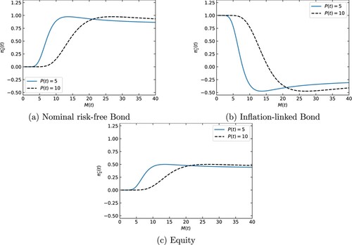For brevity, we show the wealth allocations at $P(t)=5$ in the subsequent illustrations.

Figure 1. The optimal constrained strategy for an investor with $\alpha =0$ and $\beta =0$: the optimal fraction of wealth invested in each asset as a function of $M(t)$ at time t = 20 for $P(t)=5$ and $P(t)=10$. The time-0-value of the future contributions and the minimum guarantee are $d_0=3.73$ and $g_{0,0}=3.675$, respectively. The initial wealth is $x_0=1$. The risk aversion parameter is $\gamma =3.5$. (a) shows the fraction of wealth invested in nominal risk-free bond, (b) inflation-linked bond and (c) equity.

Remark 4.1

By setting $Y(t)=P(t)$, we have $D(t)=c(e^{\delta (T-t)}-1)P(t)/\delta$. From (20(20) $Z^{\star }(t)=({\xi }_0+d_0)M(t)\mathrm{\Phi }(d_{+})+G_{\beta }(t)[1-\mathrm{\Phi }(d_{-})]$(20) ) we observe that $X^{\pi {\pi }^{\star }}(t)$ can be expressed as a function of t, $M(t)$, $P(t)$ and $P(t{)}^{1-\beta }$. Given t, we can illustrate the investment strategy $\pi {\pi }^{\star }(t)$ as a three-dimensional function when $0<\beta <1$ or a two-dimensional function when $\beta \in \{0,1\}$. We focus our illustrations on cases where $\beta \in \{0,1\}$.

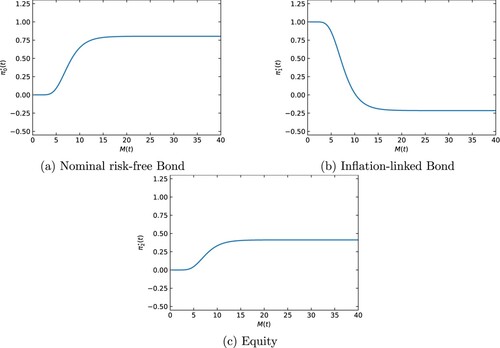
We note that in (18(18) $X^{\star }(T):=max(({\xi }_0+d_0)M(T),G_{\beta }(T)),$(18) ) Component iv is independent of the money illusion parameters α and β, as well as the investor's risk aversion γ and their level of minimum guarantee $G_{\beta }(T)$. To better focus on the impact of money illusion and its interaction with the investor's risk aversion and minimum guarantee, we update our baseline parameterization by setting c = 0 and bring forward the future contributions to time t = 0 such that $x_0=4.73$ to ensure that Assumption 3.2 is met. Figure 2 shows the optimal asset proportions in each asset as a function of $M(t)$ at $P(t)=5$ under the updated parameterization.

Figure 2. The optimal constrained strategy for an investor with $\alpha =0$ and $\beta =0$: the optimal fraction of wealth invested in each asset as a function of $M(t)$ at time t = 20, given $P(t)=5$. The contribution rate is c = 0 and which gives $d_0=0$. The minimum guarantee is determined such that $g_{0,0}=3.675$. The initial wealth is $x_0=4.73$. The risk aversion parameter is $\gamma =3.5$. (a) shows the fraction of wealth invested in nominal risk-free bond, (b) inflation-linked bond and (c) equity.

In (22(22) $\begin{array}{rl}\pi {\pi }^{\star }(t)& =\underset{\mathrm{Component}\mathrm{i}}{\underbrace{\frac{1}{\gamma }({\xi }_0+d_0)\mathrm{\Phi }(d_{+})(\sigma {\sigma }^{\mathrm{\prime }}{)}^{-1}\theta \theta \frac{M(t)}{X^{\pi {\pi }^{\star }}(t)}}}\\ & \underset{\mathrm{Component}\mathrm{ii}}{\underbrace{+\frac{\gamma -1}{\gamma }(1-\alpha )({\xi }_0+d_0)\mathrm{\Phi }(d_{+})(\sigma {\sigma }^{\mathrm{\prime }}{)}^{-1}\sigma {\sigma }_P\frac{M(t)}{X^{\pi {\pi }^{\star }}(t)}}}\\ & \underset{\mathrm{Component}\mathrm{iii}}{\underbrace{+(1-\beta )(1-\mathrm{\Phi }(d_{-}))(\sigma {\sigma }^{\mathrm{\prime }}{)}^{-1}\sigma {\sigma }_P\frac{G_{\beta }(t)}{X^{\pi {\pi }^{\star }}(t)}}}\\ & \underset{\mathrm{Component}\mathrm{iv}}{\underbrace{-(\sigma {\sigma }^{\mathrm{\prime }}{)}^{-1}\sigma {\sigma }_Y\frac{D(t)}{X^{\pi {\pi }^{\star }}(t)}}}\end{array}$(22) ), we notice that the fraction of wealth allocated to asset i for $i=2,\dots ,d$ remains unimpacted by money illusion. It is governed by the risk aversion of the investor γ and the derivative of the embedded option, $\mathrm{\Phi }(d_{+})$ which is dependent on t, $M(t)$ and $G_{\beta }(t)$ (see (21(21) $\begin{array}{rl}& d_{\pm }=\frac{\log (({\xi }_0+d_0)M(t)/G_{\beta }(t))\pm \frac{1}{2}{\nu }^2(T-t)}{\nu \sqrt{T-t}},\\ & \nu =\Vert \sigma {\sigma }_M-(1-\beta )\sigma {\sigma }_P\Vert .\end{array}$(21) )). Therefore, we center our discussion around the fraction of wealth allocated to ILB ${\pi }_1^{\star }(t)$, noting that the change in ${\pi }_1^{\star }(t)$ due to α and β is always offset by ${\pi }_0^{\star }(t)$.

Figure 3 shows the fraction of wealth allocated to ILB under different levels of money illusions on both aspects as indicated by α and β. As seen in (22(22) $\begin{array}{rl}\pi {\pi }^{\star }(t)& =\underset{\mathrm{Component}\mathrm{i}}{\underbrace{\frac{1}{\gamma }({\xi }_0+d_0)\mathrm{\Phi }(d_{+})(\sigma {\sigma }^{\mathrm{\prime }}{)}^{-1}\theta \theta \frac{M(t)}{X^{\pi {\pi }^{\star }}(t)}}}\\ & \underset{\mathrm{Component}\mathrm{ii}}{\underbrace{+\frac{\gamma -1}{\gamma }(1-\alpha )({\xi }_0+d_0)\mathrm{\Phi }(d_{+})(\sigma {\sigma }^{\mathrm{\prime }}{)}^{-1}\sigma {\sigma }_P\frac{M(t)}{X^{\pi {\pi }^{\star }}(t)}}}\\ & \underset{\mathrm{Component}\mathrm{iii}}{\underbrace{+(1-\beta )(1-\mathrm{\Phi }(d_{-}))(\sigma {\sigma }^{\mathrm{\prime }}{)}^{-1}\sigma {\sigma }_P\frac{G_{\beta }(t)}{X^{\pi {\pi }^{\star }}(t)}}}\\ & \underset{\mathrm{Component}\mathrm{iv}}{\underbrace{-(\sigma {\sigma }^{\mathrm{\prime }}{)}^{-1}\sigma {\sigma }_Y\frac{D(t)}{X^{\pi {\pi }^{\star }}(t)}}}\end{array}$(22) ), the money illusion parameter α reduces Component ii, i.e. reduces the fraction of wealth allocated to ILB. The reduction stemmed from the fact that a money-illusioned investor does not factor into full account inflation risk in evaluating utility of their wealth (aspect A). The effect is more pronounced for higher values of $M(t)$ where the unconstrained component of the portfolio plays a more prominent role. When the value of $M(t)$ is low, the investment strategy is tilted towards Component iii in order to secure the minimum guarantee. Such impact is observed both in the presence and the absence of money illusion concerning the minimum guarantee, β (aspect B). However, the money illusion parameter β changes the composition of Component iii. A non-illusioned investor sets their minimum guarantee in line with inflation, thus allocating their wealth to ILB to secure the minimum guarantee when $M(t)$ is low. On the contrary, a fully illusioned investor allocates their wealth to the nominal risk-free bond to secure a constant lower bound.

Figure 3. The optimal proportion of wealth in ILB for as a function of $M(t)$ at time t = 20 for (a) of $\beta =0$ and (b) $\beta =1$.

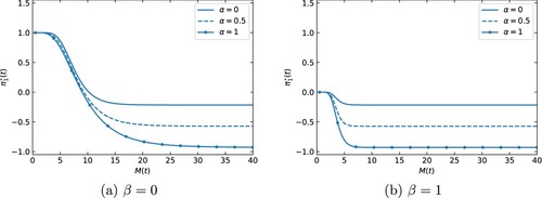
Figure 4 shows the fraction of wealth allocated to ILB under different risk aversion parameters γ and money illusion parameter α, whose impacts are more pronounced in the unconstrained component of the overall investment strategy. Specifically, the risk aversion of the investor affects Component i and ii. A higher risk aversion value (e.g. $\gamma =5$) means the investor has a lower tolerance for risks. This translates to a higher proportion of wealth invested in ILB. Its impact is particularly evident when the values of $M(t)$ are high (the dashed lines are above the solid line, with differences being more pronounced at the RHS of Figure 4).

Figure 4. The optimal proportion of wealth in ILB for as a function of $M(t)$ at time t = 20 for $\alpha \in \{0,1\}$ and $\gamma \in \{3.5,5\}$.

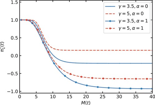
On the other hand, having $\alpha >0$ means the investor evaluates utility from a mix of nominal and real wealth due to money illusion. This reduces their allocation to ILB (the ‘o’-marked lines are below the unmarked lines) because ILB is no longer regarded as a risk-free asset under a money-illusioned perspective in aspect A.

Figure 5 shows the fraction of wealth allocated to ILB under different levels of minimum guarantee (as indicated by their initial values, which we discuss later) and money illusion parameter β. The impacts of these variables are more pronounced when the overall investment strategy is tilted towards its guarantee hedging component (Component iii). Suffering money illusion in aspect B ($\beta >0$) causes the investor to set a partial inflation-indexed minimum target. This then translates to a partial hedge, reducing the allocation to ILB towards zero as $\beta =1$ (the diamond-marked lines approach 0 on the LHS). For low values of $M(t)$, the investment strategy prescribes a higher proportion of wealth in ILB up to $1-\beta$ in order to secure the minimum guarantee $G_{\beta }(T)$ which is linked to $1-\beta$ power of the price index. The speed at which the optimal strategy converges to a $1-\beta$ fraction of wealth in ILB is influenced by the level of the minimum guarantee.

Figure 5. The optimal proportion of wealth in ILB for as a function of $M(t)$ at time t = 20 for $\beta \in \{0,1\}$ and $g_{\beta ,0}\in \{2.756,3.675\}$.

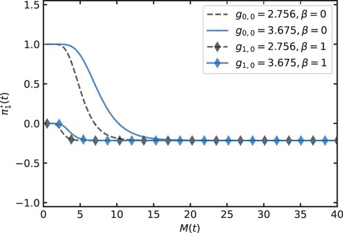
Figure 5 also shows two levels of minimum guarantee with initial values of 3.675 (the solid line) and 2.756 (the dashed line)¹². The former corresponds to the initial value of the baseline minimum guarantee; the latter corresponds to the initial value of the minimum guarantee with a lower k = 0.5 under $\beta =0$. A high value of income stream k prompts earlier deviation away from the unconstrained counterpart towards a $1-\beta$ fraction of wealth in ILB (the dashed lines are shifted toward left). In the limiting case where $g_{\beta ,0}=0$, the optimal investment strategy is reduced to just the unconstrained component, as the minimum guarantee is no longer in effect (not shown in the figure).

4.2. Cost(s) of money illusion

When money illusion is perceived as irrational behavior by a rational investor, it results in a suboptimal investment strategy that does not fully account for the inflation risk. As discussed, the investment strategy of the investor is influenced by the extent of their money illusion in two aspects: (A) the utility evaluation of their real wealth at retirement (as measured by α) and (B) the amount set aside to secure a real income stream at retirement (as measured by β). The resultant strategy under money illusion therefore implies a loss in welfare for the investor. In addition, the resultant strategy may put the investor at risk of not having enough wealth at time T to secure an inflation-indexed income stream in retirement, i.e. $G_0(T)$.

4.2.1. Certainty equivalence loss

We calculate the loss in expected utility perceived by an investor implementing the suboptimal investment strategy as a result of suffering from money illusion in aspect A which impacts their utility evaluation ($\alpha >0$). The cost is expressed in terms of certainty equivalence loss. The derivation of the expected value and certainty equivalence loss for an investor following a suboptimal strategy due to money illusion is detailed in Appendix 2.

Suffering money illusion in aspect A affects the unconstrained component of the investment strategy. Specifically, it reduces the proportion in ILB that provides hedging against inflation risk. The impact of certainty equivalence loss is more severe for more risk averse investors (Figure 6(a)). For example, the certainty equivalent loss for an investor with $\gamma =5$ is 11.2% compared to 7.6% for an investor with $\gamma =3.5$. This is because a high risk averse investor places a higher emphasis on hedging inflation risk. Having money illusion $\alpha >0$ hinders them from fully hedging inflation risk.

Figure 6. The loss of certainty equivalent as a function of α for (a) various levels of γ, (b) various levels of $g_{0,0}$, and (c) various levels of β.

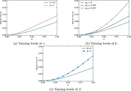
Figure 6(b) shows that the certainty equivalent loss is confined for an investor when a minimum guarantee requirement is introduced. The extent of losses diminishes as the level of minimum guarantee increases. For the unconstrained investor, the loss of utility is 19.5%. As we increase the constraint (e.g. increasing the initial value of the minimum guarantee to 3.675), the investor suffers a smaller loss in certainty equivalent at 7.6%. This is because a high level of minimum guarantee requirement prompts a more prominent role of Component iii and inevitably diminishes the role of Component ii that is dependent on α. Therefore, the inclusion of a minimum guarantee moderates the extent of certainty equivalent loss due to α. Incorporating a minimum guarantee, however, introduces an additional point of vulnerability towards the money illusion via β.

For an investor who suffers money illusion when determining the level of minimum guarantee, we observe a larger extent of loss for a higher level of β. $\beta >0$ indicates that the investor sets a partial inflation-indexed minimum guarantee, or a risk-free minimum guarantee (when $\beta =1$). As Donnelly et al. (2022) discussed, constraining the terminal wealth implies that the investor is more risk averse than the risk preference implied by γ. The investor with $\beta =1$ targets a risk-free minimum, which results in an even more risk averse constrained strategy than an investor with $\beta =0$. The former investor therefore suffers a larger extent of loss.

Table 1 summarizes the certainty equivalent loss with respect to $\alpha =0$ across different scenarios. The extent of loss increases with the value of money illusion parameter α.

Table 1. Certainty equivalent loss with respect to $\alpha =0$. The baseline parameters are $\gamma =3.5$, $g_{0,0}=3.675$ and $\beta =0$.

		α
		0	0.25	0.5	0.75	1
γ	2	0%	0.2%	0.8%	1.6%	2.7%
	3.5	0%	0.7%	2.6%	5.0%	7.6%
	5	0%	1.4%	4.4%	7.8%	11.2%
$g_{0,0}$	0${}^{\mathrm{a}}$	0%	1.3%	5.3%	11.5%	19.5%
	2.756	0%	1.0%	3.6%	7.1%	11.0%
	3.675	0%	0.7%	2.6%	5.0%	7.6%
	4.594	0%	0.3%	1.1%	2.1%	3.1%
β	0	0%	0.7%	2.6%	5.0%	7.6%
	0.5	0%	0.9%	3.6%	7.0%	10.5%
	1	0%	1.0%	4.2%	8.9%	14.4%

Note: ${}^{\mathrm{a}}$An unconstrained strategy.

4.2.2. Probability of shortfall

Being mindful of inflation risk, the rational investor targets a stream of income indexed to inflation in retirement. However, this exposes the investor to money illusion as they formulate their investment strategy to meet the minimum guarantee requirement (aspect B). We assume β represents the degree of money illusion in provisioning for inflation in their future income stream. Investors who suffer money illusion $\beta >0$ mis-specify their guarantee level without taking into full account the impact of inflation risk on their future income stream. This results in a strategy that engages in partial (or no) inflation hedging, which provides no meaningful protection against the inflation-indexed minimum guarantee. We refer to the event of failing to secure the amount needed to purchase the real income stream as the shortfall, and evaluate the shortfall probability as $\mathbb{P}(X^{\pi {\pi }^{\star }}(T)<G_0(T))$.

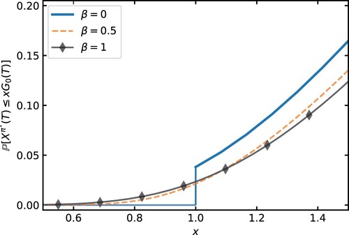
An investor who suffers money illusion in the aspect of provisioning for inflation in their future income stream, i.e. $\beta >0$ set up their investment strategy observing the minimum guarantee requirement $G_{\beta }(T)$ instead of $G_0(T)$. This exposes them to the risk of not having enough real wealth to secure a real income stream in retirement (Figure 7). Unlike the certainty equivalent loss, shortfall probabilities exhibit a dichotomous behavior (see Remark 4.2) with respect to β.

Figure 7. The cumulative probability density function of the optimal constrained strategies achieving at least x unit of the non-illusioned minimum guarantee $G_0(T)$ for various levels of β.

Remark 4.2

Consider the shortfall probability: (23) $\begin{array}{rl}& \mathbb{P}(X^{\pi {\pi }^{\star }}(T)<G_0(T))=\mathbb{P}(max(({\xi }_0+d_0)M(T),G_{\beta }(T))<G_0(T))\\ & =\mathbb{P}(({\xi }_0+d_0)M(T)<G_0(T),G_{\beta }(T)<G_0(T))\\ & =\{\begin{array}{ll}\mathbb{P}(({\xi }_0+d_0)M(T)<G_0(T),G_0(T)<G_0(T))& \text{if }\beta =0,\\ \mathbb{P}(({\xi }_0+d_0)M(T)<G_0(T),G_{\beta }(T)<G_0(T))& \text{if }\beta >0.\end{array}\end{array}$(23) We first consider the case of $\beta =0$. Since the event $G_0(T)<G_0(T)$ is $\{\mathrm{\varnothing }\}$, we have $\mathbb{P}(X^{\pi {\pi }^{\star }}(T)<G_0(T))=0$. When $\beta >0$, $\mathbb{P}(X^{\pi {\pi }^{\star }}(T)<G_0(T))=\mathbb{P}(\log (M(T)/G_0(T))<-\log ({\xi }_0+d_0)\log (G_{\beta }(T)/G_0(T))<1)>0$. We note that $\log (M(T)/G_0(T))$ and $\log (G_{\beta }(T)/G_0(T))$ are jointly normally distributed because both are linear combinations of $\mathbf{W}(T)$, a d-dimensional brownian motion. Therefore, the shortfall probability exhibits a dichotomous nature such that (24) $\mathbb{P}(X^{\pi {\pi }^{\star }}(T)<G_0(T))\{\begin{array}{ll}=0& \text{if}\beta =0,\\ >0& \text{if}\beta >0.\end{array}$(24)

Table 2 provides a summary of shortfall probabilities across different scenarios. A low risk aversion strategy typically results in a more aggressive investment strategy. As shown in Table 2, when $\beta =1$, the shortfall probabilities increase from 1.3% to 5.3% as γ decreases from 5 to 2, respectively. Increasing the level of minimum guarantee (as measured by $g_{\beta ,0}$) increases the difficulty of meeting the minimum guarantee constraint. This is evident by the increase in shortfall probabilities for all β values. As discussed in Section 4.2.1, an investor suffering money illusion in the aspect of utility evaluation $\alpha >0$ adopts a ‘more’ risky investment strategy in real terms as it does not place a sufficient fraction of wealth in the real risk-free asset (i.e. ILB). Therefore the impact of $\alpha >0$ bears much resemblance to the impact due to differences in γ. A fully-illusioned strategy ($\alpha =1$) results in a more aggressive investment strategy, which leads to a higher shortfall probability. From Remark 4.2, the shortfall probabilities can be evaluated as the joint probabilities of two lognormal processes ($M(T)/G_0(T)$ and $G_{\beta }(T)/G_0(T)$) when $\beta >0$. The shortfall probabilities do not monotonically increase or decrease with β.

Table 2. The probability of shortfall, $\mathbb{P}(X^{\pi {\pi }^{\star }}(T)<G_0(T))$. The baseline parameters are $\gamma =3.5$, $g_{0,0}=3.675$ and $\alpha =0$.

		β
		0	0.25	0.5	0.75	1
γ	2	–	5.1%	5.2%	5.2%	5.3%
	3.5	–	2.2%	2.1%	2.2%	2.3%
	5	–	1.0%	1.0%	1.1%	1.3%
$g_{\beta ,0}$	2.756	–	0.5%	0.5%	0.5%	0.5%
	3.675	–	2.2%	2.1%	2.2%	2.3%
	4.594	–	8.8%	8.7%	9.0%	10.2%
α	0	–	2.2%	2.1%	2.2%	2.3%
	0.5	–	4.3%	4.0%	3.8%	3.8%
	1	–	7.0%	6.7%	6.4%	6.1%

5. Conclusion

Pre-retiree investors face a wide range of investment decisions in planning for retirement in managing investment risk and inflation risk. Traditionally, the problem of finding optimal investment strategies has been dominated by the maximization of expected utility in a nominal market or a real market entirely. However, the explicit examination of the costs associated with misjudging inflation risk, also known as money illusion, from the perspective of pre-retiree investors, has only recently been explored by Lioui (2013) and Wei and Yang (2023).

In this paper, we extend the study of money illusion to investment strategies that are subject to a minimum guarantee constraint. Specifically, we derive the optimal investment strategy for investors experiencing money illusion in two key areas: (A) evaluating the utility of wealth and (B) determining the minimum guarantee constraint. Our findings reveal that the impact of these two aspects of money illusion is largely isolated within their respective components. Aspect A influences the ‘unconstrained’ component of the overall strategy, which governs the riskiness of the investment strategy while, if applicable, still accounting for the need for hedging necessitated by the minimum guarantee. On the other hand, Aspect B affects the dynamics of the minimum guarantee and its hedging component.

In the absence of a minimum guarantee, our results align with existing literature, indicating that investors with money illusion tend to reduce the proportion of wealth invested in inflation-linked bonds in favor of nominal bonds (Lioui & Tarelli, 2023). Furthermore, for more risk-averse investors, the welfare loss resulting from money illusion is greater (Wei & Yang, 2023). However, our results suggest that the introduction of a minimum guarantee can suppress welfare loss. Specifically, a higher level of minimum guarantee results in a smaller extent of welfare loss. Nonetheless, incorporating a minimum guarantee exposes the investor to the second aspect of money illusion described above. Mis-specifying inflation risk in the determination of the minimum guarantee renders it ineffective and directly puts the investor at risk of not meeting the inflation-indexed guarantee.

In conclusion, an investor's ability to consider and effectively account for inflation risk has a substantial impact on their investment strategy and retirement outcomes. This is particularly pertinent for investors seeking a minimum guarantee. Providers of retirement savings products should take these factors into account when offering advice and designing suitable investment options.

Our paper can be extended in several ways. To make our setting more practical, we can include mortality risk or unhedgeable stochastic labor income into the model, albeit this will render the market incomplete. Additionally, as alluded to in Appendix 3, the presence of money illusion may have an interesting impact on the investor's decision regarding optimal retirement time. We believe that this can be explored in greater detail in future research.

Disclosure statement

No potential conflict of interest was reported by the author(s).

Notes

1 The concept of money illusion is supported by empirical and experimental evidence (see e.g.  Fehr & Tyran, 2001, 2007; Modigliani & Cohn, 1979)

2 In practice, the real return is known only approximately at the time of sale or redemption, since the indexation of the payments with the price index is not perfect: for practical reasons, the values of the price index used for indexation of real life inflation-linked bonds are generally lagged by at least three months.

3 ${\mu }_Y$ can be adjusted to be a deterministic function that captures the hump-shaped pattern in labor income over the life cycle.

4 This configuration allows the labor income of the investor to capture inflation risk as well as other idiosyncratic risks in the market (see e.g. Barucci & Marazzina, 2012). Setting $\sigma {\sigma }_Y=[10\dots 0{]}^{\mathrm{\prime }}$, we recover a labor process that depends on inflation only, which is the case studied by Zhang and Ewald (2010).

5 The power utility function includes the logarithmic utility function $U(x)=\log (x)$ for $\gamma =1$. To get to the limiting case, one can add a constant to the utility function such that $U(x)=(x^{1-\gamma }-1)/(1-\gamma )$. As Jensen and Sørensen (2001) pointed out, this has no consequence for preference but leads to a more complicated notation elsewhere.

6 We adopt this assumption to obtain a simpler and explicit result, highlighting the impact of money illusion in the presence of a minimum guarantee.

7 Finkelstein and Poterba (2004) found over 90% annuitants in UK choose to buy a level-life annuity despite preferring an inflation-indexed annuity before purchase.

8 To verify, we can consider the limiting case where k = 0 (see Remark 3.7).

9 Affine term structure, whilst being flexible in modeling realistic features of economics variables (e.g. mean reversion of inflation rate), are prone to estimation errors and in-sample overfitting (Sarno et al., 2016). Here, we consider the investment problem under money illusions in the presence of a minimum guarantee constraint. The unconstrained problem is obtained as the limiting case where the constraint is set to zero.

10 This assumption follows by two reasons. First, as the dynamic of the labor income process matches the dynamics of the price process, the payment amount of the annuity k can be interpreted as the replacement ratio, i.e. the ratio of labor income. Our baseline parameters assume the investor requires a replacement rate of at least two-thirds at retirement. This is broadly consistent with the findings of Byrne et al. (2007) that a contribution rate of 0.16 is required to achieve a two-thirds replacement ratio after 40 years of savings. Second, by setting $\sigma {\sigma }_Y$ as $\sigma {\sigma }_P$, there exists one-to-one relationships between $D(t)$, $P(t)$ and $G_{\beta }(t)$, reducing the dimensions needed for numerical illustrations (see Remark 4.1).

11 We choose the risk aversion parameters based on the empirical findings of Khemka et al. (2021). According to Khemka et al. (2021), the underlying risk aversion of life-cycle glide path funds offered in the US, UK, Australia and Denmark range between 2 and 5.

12 Recall (14(14) $$\begin{gathered} G_{\beta }(t)=\frac{k}{{\eta }_{\beta }}[e^{{\eta }_{\beta }(T^{{ \\ }^{\prime }}-t)}-e^{{\eta }_{\beta }(T-t)}]P(t{)}^{1-\beta }, \end{gathered}$$(14) ), the level of minimum guarantee is determined by (i) the value of income stream payment k, (ii) the length of income stream $$\begin{gathered} T^{{ \\ }^{\prime }}-T \end{gathered}$$, and (iii) the money illusion parameter β. In our numerical illustrations, we keep $$\begin{gathered} T^{{ \\ }^{\prime }} \end{gathered}$$ constant and adjust the value of k for different values of β to ensure that $g_{\beta ,0}=g_{0,0}$ for a given level of minimum guarantee.

Appendices

Appendix 1.

Proofs

A.1. Proof of Proposition 2.1

Proof.

By the definition of $D(t)$, we have $\begin{array}{rl}D(t)& =\mathrm{cY}(t){\mathbb{E}}_t\left[{\int }_t^T\frac{Y(s)}{Y(t)}\frac{H(s)}{H(t)}\mathrm{d}s\right]\\ & =\mathrm{cY}(t){\int }_t^T{\mathbb{E}}_t\left[\frac{Y(s)}{Y(t)}\frac{H(s)}{H(t)}\right]\mathrm{d}s\\ & =\mathrm{cY}(t){\int }_t^T{e}^{\delta (s-t)}\mathrm{d}s\\ & =\frac{c}{\delta }[e^{\delta (T-t)}-1]Y(t)\end{array}$where $\delta ={\mu }_Y-r_{\mathrm{N}}-\sigma {\sigma }_Y^{\mathrm{\prime }}\theta \theta$. Then, differentiating (7(7) $D(t)=\frac{c}{\delta }[e^{\delta (T-t)}-1]Y(t),$(7) ), we have $\begin{array}{rl}\mathrm{d}D(t)& =d(\frac{c}{\delta }[e^{\delta (T-t)}-1]Y(t))\\ & =\frac{c}{\delta }[e^{\delta (T-t)}-1]\mathrm{d}Y(t)-\frac{c}{\delta }Y(t)\delta e^{\delta (T-t)}\mathrm{d}t\\ & =D(t)[(r_{\mathrm{N}}+\sigma {\sigma }_Y^{\mathrm{\prime }}\theta \theta )\mathrm{d}t+\sigma {\sigma }_Y^{\mathrm{\prime }}\mathrm{d}\mathbf{W}(t)]-\mathrm{cY}(t)\mathrm{d}t\end{array}$

A.2. Proof of Proposition 3.3

Proof.

The proof is adapted from Donnelly et al. (2015) and Grossman and Zhou (1996).

Assume that there exists ${\xi }_0$ so that the budget constraint (9(9) $\mathbb{E}(H(T)X^{\pi \pi }(T))\le x_0+d_0.$(9) ) is satisfied with equality by $X^{\star }(T)$.

For the investor's utility function, the first derivative $U^{\mathrm{\prime }}(x)=x^{\gamma -1}$, which is a strictly decreasing function, has a strictly decreasing inverse I with $I(x):=x^{\frac{1}{\gamma -1}},x>0.$We can show that for the constant ${\lambda }_1:={({\xi }_0+d_0)}^{\gamma -1}{e}^{\gamma \mathrm{\Gamma T}},$where $\begin{array}{rl}\mathrm{\Gamma }& =-\frac{\gamma -1}{\gamma }{r}_{\mathrm{N}}+\frac{1}{2}\frac{\gamma -1}{\gamma }(-\frac{1}{\gamma })\Vert \theta \theta {\Vert }^2\\ & +\frac{\gamma -1}{\gamma }(1-\alpha ){\mu }_P+\frac{1}{2}(\frac{\gamma -1}{\gamma }(1-\alpha ))(\frac{\gamma -1}{\gamma }(1-\alpha )-1)\Vert \sigma {\sigma }_P{\Vert }^2\\ & -{\left(\frac{\gamma -1}{\gamma }\right)}^2(1-\alpha )\theta {\theta }^{\mathrm{\prime }}\sigma {\sigma }_P\end{array}$we have $({\xi }_0+d_0)M(T)/P(T{)}^{1-\alpha }=I({\lambda }_{1}H(T)P(T{)}^{1-\alpha })$.

We work with $I({\lambda }_1({\xi }_0)H(T)P(T{)}^{1-\alpha })$ in the proof, rather than with $({\xi }_0+d_0)M(T)/P(T{)}^{1-\alpha }$ due to the properties of $I(x)$ and $U^{\mathrm{\prime }}(x)$: they are both strictly decreasing functions of x.

Let $X(T)\in [G_{\beta }(T),\mathrm{\infty })$, a.s. be any attainable terminal wealth so that $\mathbb{E}[H(T)X(T)]\le X_0$. We show that $\mathbb{E}\left[U(X(T)/P(T{)}^{1-\alpha })\right]\le \mathbb{E}\left[U(X^{\star }(T)/P(T{)}^{1-\alpha })\right],$Then, by arbitrary choice of X, $\underset{\pi \pi \in \mathcal{A}}{sup}\mathbb{E}[U(X(T)/P(T{)}^{1-\alpha })]\le \mathbb{E}[U(X^{\star }(T)/P(T{)}^{1-\alpha })]$.

From Equation (18(18) $X^{\star }(T):=max(({\xi }_0+d_0)M(T),G_{\beta }(T)),$(18) ) and using the fact that $U^{\mathrm{\prime }}$ is a strictly decreasing function, $\begin{array}{rl}{X}^{\star }(T)& =\{\begin{array}{ll}I({\lambda }_{1}H(T)P(T{)}^{1-\alpha })P(T{)}^{1-\alpha }& \text{if }I({\lambda }_{1}H(T)P(T{)}^{1-\alpha })\ge G_{\beta }(T)/P(T{)}^{1-\alpha }\\ G_{\beta }(T)& \text{if }I({\lambda }_{1}H(T)P(T{)}^{1-\alpha })<G_{\beta }(T)/P(T{)}^{1-\alpha }\end{array}\\ & =\{\begin{array}{ll}I({\lambda }_{1}H(T)P(T{)}^{1-\alpha })P(T{)}^{1-\alpha }& \text{if }{\lambda }_{1}H(T)P(T{)}^{1-\alpha }\le U^{\mathrm{\prime }}(G_{\beta }(T)/P(T{)}^{1-\alpha })\\ G_{\beta }(T)& \text{if }{\lambda }_{1}H(T)P(T{)}^{1-\alpha }>U^{\mathrm{\prime }}(G_{\beta }(T)/P(T{)}^{1-\alpha })\end{array}\end{array}$As U is a concave function, then for any $a,b\in \mathbb{R}$, $U(a)-U(b)\le U^{\mathrm{\prime }}(b)\cdot (a-b)$. In particular, $\begin{array}{rl}& U\left(\frac{X(T)}{P(T{)}^{1-\alpha }}\right)-U\left(\frac{X^{\star }(T)}{P(T{)}^{1-\alpha }}\right)\\ & \le U^{\mathrm{\prime }}\left(\frac{X^{\star }(T)}{P(T{)}^{1-\alpha }}\right)\cdot (\frac{X(T)}{P(T{)}^{1-\alpha }}-\frac{X^{\star }(T)}{P(T{)}^{1-\alpha }}),\mathrm{a}.\mathrm{s}.\end{array}$In the following, we dropped the T when it is unambiguous. Take expectations in the above inequality to get $\begin{array}{rl}& \mathbb{E}(U(X/P^{1-\alpha })-U(X^{\star }/P^{1-\alpha }))\\ & \le \mathbb{E}(U^{\mathrm{\prime }}(X^{\star }/P^{1-\alpha })\cdot (X/P^{1-\alpha }-X^{\star }/P^{1-\alpha }))\\ & \le \mathbb{E}(U^{\mathrm{\prime }}(X^{\star }/P^{1-\alpha })\cdot (X/P^{1-\alpha }-X^{\star }/P^{1-\alpha })|{\lambda }_{1}H{P}^{1-\alpha }\le U^{\mathrm{\prime }}(G_{\beta }/P^{1-\alpha }))\\ & \cdot \mathbb{P}[{\lambda }_{1}H{P}^{1-\alpha }\le U^{\mathrm{\prime }}(G_{\beta }/P^{1-\alpha })]\\ & +\mathbb{E}(U^{\mathrm{\prime }}(X^{\star }/P^{1-\alpha })\cdot (X/P^{1-\alpha }-X^{\star }/P^{1-\alpha })|{\lambda }_{1}H{P}^{1-\alpha }>U^{\mathrm{\prime }}(G_{\beta }/P^{1-\alpha }))\\ & \cdot \mathbb{P}[{\lambda }_{1}H{P}^{1-\alpha }>U^{\mathrm{\prime }}(G_{\beta }/P^{1-\alpha })]\end{array}$Observe that on the event ${\lambda }_{1}H{P}^{1-\alpha }\le U^{\mathrm{\prime }}(G_{\beta }/P^{1-\alpha })$, $U^{\mathrm{\prime }}(X^{\star }/P^{1-\alpha })=U^{\mathrm{\prime }}(I({\lambda }_{1}H{P}^{1-\alpha }))={\lambda }_{1}H{P}^{1-\alpha }$so that $\begin{array}{rl}& \mathbb{E}(U^{\mathrm{\prime }}(X^{\star }/P^{1-\alpha })\cdot (X/P^{1-\alpha }-X^{\star }/P^{1-\alpha })|{\lambda }_{1}H{P}^{1-\alpha }\le U^{\mathrm{\prime }}(G_{\beta }/P^{1-\alpha }))\\ & =\mathbb{E}({\lambda }_{1}H{P}^{1-\alpha }\cdot (X/P^{1-\alpha }-X^{\star }/P^{1-\alpha })|{\lambda }_{1}H{P}^{1-\alpha }\le U^{\mathrm{\prime }}(G_{\beta }/P^{1-\alpha })).\end{array}$Next, observe that on the event ${\lambda }_{1}H{P}^{1-\alpha }>U^{\mathrm{\prime }}(G_{\beta }/P^{1-\alpha })$, since $X\in [G_{\beta },\mathrm{\infty })$ a.s., then $X/P^{1-\alpha }-X^{\star }/P^{1-\alpha }=X/P^{1-\alpha }-G_{\beta }/P^{1-\alpha }\ge 0$and $U^{\mathrm{\prime }}(X^{\star }/P^{1-\alpha })=U^{\mathrm{\prime }}(G_{\beta }/P^{1-\alpha })<{\lambda }_{1}H{P}^{1-\alpha }.$Upon multiplying both sides of the inequality $U^{\mathrm{\prime }}(X^{\star }/P^{1-\alpha })<{\lambda }_{1}H{P}^{1-\alpha }$ by the positive random variable $X/P^{1-\alpha }-X^{\star }/P^{1-\alpha }$ and taking expectation, we find that $\begin{array}{rl}& \mathbb{E}(U^{\mathrm{\prime }}(X^{\star }/P^{1-\alpha })\cdot (X/P^{1-\alpha }-X^{\star }/P^{1-\alpha })|{\lambda }_{1}H{P}^{1-\alpha }>U^{\mathrm{\prime }}(G_{\beta }/P^{1-\alpha }))\\ & \le \mathbb{E}({\lambda }_{1}H{P}^{1-\alpha }\cdot (X/P^{1-\alpha }-X^{\star }/P^{1-\alpha })|{\lambda }_{1}H{P}^{1-\alpha }>U^{\mathrm{\prime }}(G_{\beta }/P^{1-\alpha })).\end{array}$In summary, we find that $\mathbb{E}(U^{\mathrm{\prime }}(X^{\star }/P^{1-\alpha })\cdot (X/P^{1-\alpha }-X^{\star }/P^{1-\alpha }))\le \mathbb{E}({\lambda }_{1}H{P}^{1-\alpha }\cdot (X/P^{1-\alpha }-X^{\star }/P^{1-\alpha })).$As both $X(T)$ and $X^{\star }(T)$ satisfy the budget constraint (9(9) $\mathbb{E}(H(T)X^{\pi \pi }(T))\le x_0+d_0.$(9) ), the last line of the above inequality can be evaluated as $\mathbb{E}({\lambda }_{1}H{P}^{1-\alpha }\cdot (X/P^{1-\alpha }-X^{\star }/P^{1-\alpha }))=\mathbb{E}({\lambda }_{1}H\cdot (X-X^{\star }))\le {\lambda }_1\cdot (X_0-X_0)=0,$which means $\mathbb{E}(U(X/P^{1-\alpha })-U(X^{\star }/P^{1-\alpha }))\le 0$, as required.

A.3. Proof of Proposition 3.4

Proof.

Differentiating both sides of $Z^{\pi \pi }(t)$, we have $\begin{array}{rl}\mathrm{d}{Z}^{\pi \pi }(t)& =\mathrm{d}{X}^{\pi \pi }(t)+\mathrm{d}D(t)\\ & =Z^{\pi \pi }(t)r_{\mathrm{N}}\mathrm{d}t+(\pi {\pi }^{\mathrm{\prime }}(t)\sigma \sigma X^{\pi \pi }(t)+\sigma {\sigma }_Y^{\mathrm{\prime }}D(t))\times (\theta \theta \mathrm{d}t+\mathrm{d}\mathbf{W}(t)).\end{array}$Using Itô's rule, we find that $\mathrm{d}(H(t)Z^{\pi \pi }(t))$ is driftless, $\begin{array}{rl}\mathrm{d}(H(t)Z^{\pi \pi }(t))& =H(t)\mathrm{d}{Z}^{\pi \pi }(t)+Z^{\pi \pi }(t)\mathrm{d}H(t)+\mathrm{d}H(t)\mathrm{d}{Z}^{\pi \pi }(t)\\ & =H(t)(X^{\pi \pi }(t)\pi {\pi }^{\mathrm{\prime }}(t)\sigma \sigma +D(t)\sigma {\sigma }_Y^{\mathrm{\prime }}-Z^{\pi \pi }(t)\theta {\theta }^{\mathrm{\prime }})\mathrm{d}\mathbf{W}(t)\end{array}$which implies that $H(t)Z^{\pi \pi }(t)$ is a martingale.

A.4. Proof of Proposition 3.6

Proof.

Applying Itô's lemma on (20(20) $Z^{\star }(t)=({\xi }_0+d_0)M(t)\mathrm{\Phi }(d_{+})+G_{\beta }(t)[1-\mathrm{\Phi }(d_{-})]$(20) ) and collecting the diffusion term, we obtain $\frac{\mathrm{\partial }{Z}^{\star }(t)}{\mathrm{\partial }M(t)}M(t)\sigma {\sigma }_M^{\mathrm{\prime }}\mathrm{d}\mathbf{W}(t)+(1-\beta )\frac{\mathrm{\partial }{Z}^{\star }(t)}{\mathrm{\partial }{G}_{\beta }(t)}{G}_{\beta }(t)\sigma {\sigma }_P^{\mathrm{\prime }}\mathrm{d}\mathbf{W}(t).$Comparing it with the diffusion term of the total wealth process dynamics of the investor (19(19) $Z^{\pi \pi }(t)=Z^{\pi \pi }(t)r_{\mathrm{N}}\mathrm{d}t+(X^{\pi \pi }(t)\pi {\pi }^{\mathrm{\prime }}(t)\sigma \sigma +D(t)\sigma {\sigma }_Y^{\mathrm{\prime }})\times (\theta \theta \mathrm{d}t+d\mathbf{W}(t)).$(19) ), which is $(X^{\pi {\pi }^{\star }}(t)\pi {\pi }^{\star }(t{)}^{\mathrm{\prime }}\sigma \sigma +D(t)\sigma {\sigma }_Y^{\mathrm{\prime }})\mathrm{d}\mathbf{W}(t).$Equating gives $X^{\pi {\pi }^{\star }}(t)\pi {\pi }^{\star }(t{)}^{\mathrm{\prime }}\sigma \sigma =\frac{\mathrm{\partial }{Z}^{\star }(t)}{\mathrm{\partial }M(t)}M(t)\sigma {\sigma }_M^{\mathrm{\prime }}+(1-\beta )\frac{\mathrm{\partial }{Z}^{\star }(t)}{\mathrm{\partial }{G}_{\beta }(t)}{G}_{\beta }(t)\sigma {\sigma }_P^{\mathrm{\prime }}-D(t)\sigma {\sigma }_Y^{\mathrm{\prime }}.$Solving for the optimal portfolio gives $\begin{array}{rl}\pi {\pi }^{\star }(t)& =(\sigma {\sigma }^{\mathrm{\prime }}{)}^{-1}\sigma {\sigma }_M\frac{\mathrm{\partial }{Z}^{\star }(t)}{\mathrm{\partial }M(t)}\frac{M(t)}{X^{\pi {\pi }^{\star }}(t)}+(1-\beta )(\sigma {\sigma }^{\mathrm{\prime }}{)}^{-1}\sigma {\sigma }_P\frac{\mathrm{\partial }{Z}^{\star }(t)}{\mathrm{\partial }{G}_{\beta }(t)}\frac{G_{\beta }(t)}{X^{\pi {\pi }^{\star }}(t)}-(\sigma {\sigma }^{\mathrm{\prime }}{)}^{-1}\sigma {\sigma }_Y\frac{D(t)}{X^{\pi {\pi }^{\star }}(t)}\\ & =(\sigma {\sigma }^{\mathrm{\prime }}{)}^{-1}\sigma {\sigma }_M({\xi }_0+d_0)\mathrm{\Phi }(d_{+})\frac{M(t)}{X^{\pi {\pi }^{\star }}(t)}\\ & +(1-\beta )(\sigma {\sigma }^{\mathrm{\prime }}{)}^{-1}\sigma {\sigma }_P[1-\mathrm{\Phi }(d_{-})]\frac{G_{\beta }(t)}{X^{\pi {\pi }^{\star }}(t)}-(\sigma {\sigma }^{\mathrm{\prime }}{)}^{-1}\sigma {\sigma }_Y\frac{D(t)}{X^{\pi {\pi }^{\star }}(t)}\\ & =\frac{1}{\gamma }(\sigma {\sigma }^{\mathrm{\prime }}{)}^{-1}\theta \theta ({\xi }_0+d_0)\mathrm{\Phi }(d_{+})\frac{M(t)}{X^{\pi {\pi }^{\star }}(t)}\\ & +\frac{\gamma -1}{\gamma }(1-\alpha )(\sigma {\sigma }^{\mathrm{\prime }}{)}^{-1}\sigma {\sigma }_P({\xi }_0+d_0)\mathrm{\Phi }(d_{+})\frac{M(t)}{X^{\pi {\pi }^{\star }}(t)}\\ & +(1-\beta )(\sigma {\sigma }^{\mathrm{\prime }}{)}^{-1}\sigma {\sigma }_P[1-\mathrm{\Phi }(d_{-})]\frac{G_{\beta }(t)}{X^{\pi {\pi }^{\star }}(t)}-(\sigma {\sigma }^{\mathrm{\prime }}{)}^{-1}\sigma {\sigma }_Y\frac{D(t)}{X^{\pi {\pi }^{\star }}(t)}\end{array}$where we substituted $\mathrm{\partial }{Z}^{\star }(t)/\mathrm{\partial M}(t)=({\xi }_0+d_0)\mathrm{\Phi }(d_{+})$ and $\mathrm{\partial }{Z}^{\star }(t)/\mathrm{\partial }{G}_{\beta }(t)=1-\mathrm{\Phi }(d_{-})$ to arrive at the second equation.

Appendix 2.

Derivation of expected utility and certainty equivalence loss

The certainty equivalent loss, loss, incurred by following an investment strategy devised under money illusion in aspect A is given by (A1) $\mathrm{loss}(\alpha )=\frac{\mathrm{CEW}(T;0,\beta )-\mathrm{CEW}(T;\alpha ,\beta )}{\mathrm{CEW}(T;0,\beta )},$(A1) where $\mathrm{CEW}(T;\alpha ,\beta ):=U^{-1}(\mathbb{E}[U(X^{\pi {\pi }^{\star }}(T;\alpha ,\beta )/P(T))])$ is the inverse of the expected utility of the real wealth, following the optimal investment strategy devised under potential money illusion (as measured by α and β).

When $\beta =0$, we note that $X^{\pi {\pi }^{\star }}(T;\alpha ,0)/P(T)=max(({\xi }_0+d_0)M(T;\alpha )/P(T),$ $$\begin{gathered} k(e^{{\eta }_0(T^{{ \\ }^{\prime }}-T)}-1)/{\eta }_0) \end{gathered}$$. This means the real wealth is the higher value of a log Normal random variable and a constant. Therefore, the expected utility of real wealth for $\beta =0$ can be evaluated analytically using Lemma A.1. When $\beta >0$, the closed-form expression of $\mathbb{E}[U(X^{\pi {\pi }^{\star }}(T;\alpha ,\beta )/P(T))]$ is not available. We evaluate $\mathrm{CEW}(T;\alpha ,\beta )$ and $\mathrm{loss}(\alpha )$ numerically using the Monte Carlo method.

Lemma A.1

Suppose X is a log Normal random variable such that $\log (X)$ is normally distributed with mean $m-s^2/2$ and variance $s^2$ where m and s are constants. Furthermore, suppose $V=max(\mathrm{pX},K)$ is the maximum of pX and K where p and K are constants. Then, the expected utility of V is given by (A2) $\mathbb{E}[U(V)]=\frac{1}{1-\gamma }{p}^{1-\gamma }{e}^{(1-\gamma )m-\gamma (1-\gamma )s^2/2}\mathrm{\Phi }(d_{\ast }+(1-\gamma )s)+\frac{1}{1-\gamma }{K}^{1-\gamma }\mathrm{\Phi }(-d_{\ast })$(A2) where (A3) $d_{\ast }=\frac{\log (p/K)+m-s^2/2}{s}.$(A3)

Appendix 3.

Sensitivity analysis of retirement time

In our model, we have assumed that the retirement time, T, is a constant given exogenously. However, there exists a strand of literature on retirement savings in which the retirement time is modeled as the investor's decision and therefore can be optimized (see e.g. Barucci & Marazzina, 2012; Choi et al., 2008; Ding & Marazzina, 2022, 2024; Farhi & Panageas, 2007). The impact of money illusion on the investor's optimal choice of retirement time presents itself as an intriguing question, which we leave for future research. In this section, we provide a brief sensitivity analysis showcasing the impacts of retirement time T.

We note that the retirement date wields its influence in both $d_0$ and $g_{\beta ,0}$. A longer retirement time simultaneously implies a longer period for contributions into savings and hence increases the present value of future contributions. It also implies a shorter period of income stream requirement post-retirement and hence decreases the present value of the minimum guarantee (and vice versa). For instance, as T increases from 40 to 42, the present value of future contributions increases to 3.833, and the present value of the minimum guarantee decreases to 3.216. We found $g_{\beta ,0}$ is more sensitive to changes in T than $d_0$. As a result, the impact of retirement time on optimal strategies is not dissimilar to the impact of k (see Section 4.1), whose influence is limited to $g_{\beta ,0}$.

Assuming baseline parameters as set out in Section 4, Table A1 summarizes the certainty equivalent loss with respect to $\alpha =0$ for different retirement times. The longer the investment horizon is, the longer the money-illusioned investor behaves suboptimally, resulting in larger extents of losses. Lastly, Table A2 provides a summary of shortfall probabilities for different retirement times. We observe that the probability of shortfall decreases with retirement time. This result can be attributed to an increase in $d_0$ and a reduction in $g_{\beta ,0}$ (see Remark 4.2).

Table D1. Certainty equivalent loss with respect to $\alpha =0$. The baseline parameters are $\gamma =3.5$, k = 0.667, $\beta =0$ and T = 40.

	α
T	0	0.25	0.5	0.75	1
38	0.0%	2.2%	4.3%	6.5%	6.6%
40	0.0%	2.6%	5.0%	7.5%	7.6%
42	0.0%	2.9%	5.6%	8.5%	8.7%

Table D2. The probability of shortfall, $\mathbb{P}(X^{\pi {\pi }^{\star }}(T)<G_0(T))$. The baseline parameters are $\gamma =3.5$, $k=0.667$, $\alpha =0$, and T = 40.

	β
T	0	0.25	0.5	0.75	1
38	–	5.4%	5.2%	5.3%	5.9%
40	–	2.2%	2.1%	2.2%	2.3%
42	–	0.9%	0.9%	0.9%	1.0%

References

- Alles, L. (2011). Design considerations for retirement savings and retirement income products. Pensions: An International Journal, 16, 4–12. https://doi.org/10.1057/pm.2010.31
- Barucci, E., & Marazzina, D. (2012). Optimal investment, stochastic labor income and retirement. Applied Mathematics and Computation, 218, 5588–5604. https://doi.org/10.1016/j.amc.2011.11.052
- Barucci, E., Marazzina, D., & Mastrogiacomo, E. (2021). Optimal investment strategies with a minimum performance constraint. Annals of Operations Research, 299, 215–239. https://doi.org/10.1007/s10479-019-03348-2
- Basak, S., & Yan, H. (2010). Equilibrium asset prices and investor behavior in the presence of money illusion. The Review of Economic Studies, 77, 914–936. https://doi.org/10.1111/roes.2010.77.issue-3
- Battocchio, P., & Menoncin, F. (2004). Optimal pension management in a stochastic framework. Insurance: Mathematics and Economics, 34, 79–95.
- Boulier, J. F., Huang, S., & Taillard, G. (2001). Optimal management under stochastic interest rates: The case of a protected defined contribution pension fund. Insurance: Mathematics and Economics, 28, 173–189.
- Brennan, M. J., & Xia, Y. (2002). Dynamic asset allocation under inflation. The Journal of Finance, 57, 1201–1238. https://doi.org/10.1111/jofi.2002.57.issue-3
- Byrne, A., Blake, D., Cairns, A., & Dowd, K. (2007). Default funds in U.K. defined-contribution plans. Financial Analysts Journal, 63, 40–51. https://doi.org/10.2469/faj.v63.n4.4748
- Chen, Z., Li, Z., & Zeng, Y. (2023). Portfolio choice with illiquid asset for a loss-averse pension fund investor. Insurance: Mathematics and Economics, 108, 60–83.
- Chen, Z., Li, Z., Zeng, Y., & Sun, J. (2017). Asset allocation under loss aversion and minimum performance constraint in a dc pension plan with inflation risk. Insurance: Mathematics and Economics, 75, 137–150.
- Choi, K. J., Shim, G., & Shin, Y. H. (2008). Optimal portfolio, consumption-leisure and retirement choice problem with ces utility. Mathematical Finance, 18, 445–472. https://doi.org/10.1111/mafi.2008.18.issue-3
- Ding, G., & Marazzina, D. (2022). The impact of liquidity constraints and cashflows on the optimal retirement problem. Finance Research Letters, 49, 103159. https://doi.org/10.1016/j.frl.2022.103159
- Ding, G., & Marazzina, D. (2024). Bankruptcy and retirement: A comparison in an optimal stopping times ordered framework. Computational and Applied Mathematics, 43, 53. https://doi.org/10.1007/s40314-023-02566-6
- Donnelly, C., Gerrard, R., Guillén, M., & Nielsen, J. (2015). Less is more: Increasing retirement gains by using an upside terminal wealth constraint. Insurance: Mathematics and Economics, 64, 259–267.
- Donnelly, C., Khemka, G., & Lim, W. (2022). Investing for retirement: Terminal wealth constraints or a desired wealth target? European Financial Management, 28, 1283–1307. https://doi.org/10.1111/eufm.v28.5
- Farhi, E., & Panageas, S. (2007). Saving and investing for early retirement: A theoretical analysis. Journal of Financial Economics, 83, 87–121. https://doi.org/10.1016/j.jfineco.2005.10.004
- Fehr, E., & Tyran, J.-R. (2001). Does money illusion matter? American Economic Review, 91, 1239–1262. https://doi.org/10.1257/aer.91.5.1239
- Fehr, E., & Tyran, J.-R. (2007). Money illusion and coordination failure. Games and Economic Behavior, 58, 246–268. https://doi.org/10.1016/j.geb.2006.04.005
- Finkelstein, A., & Poterba, J. (2004). Adverse selection in insurance markets: Policyholder evidence from the U.K. annuity market. Journal of Political Economy, 112, 183–208. https://doi.org/10.1086/379936
- Greenwald Research (2022). 2021 retirement risk survey – report of findings. Sponsored by the Society of Actuaries.
- Grossman, S., & Zhou, Z. (1996). Equilibrium analysis of portfolio insurance. Journal of Finance, 51, 1379–1403. https://doi.org/10.1111/jofi.1996.51.issue-4
- Han, N.-W., & Hung, M.-W. (2012). Optimal asset allocation for DC pension plans under inflation. Insurance: Mathematics and Economics, 51, 172–181.
- Jensen, B. A., & Sørensen, C. (2001). Paying for minimum interest rate guarantees: Who should compensate who? European Financial Management, 7, 183–211. https://doi.org/10.1111/eufm.2001.7.issue-2
- Karatzas, I., & Shreve, S. (1998). Methods of mathematical finance. Springer.
- Khemka, G., Steffensen, M., & Warren, G. J. (2021). How sub-optimal are age-based life-cycle investment products? International Review of Financial Analysis, 73, 101619. https://doi.org/10.1016/j.irfa.2020.101619
- Korn, R. (2005). Optimal portfolios with a positive lower bound on final wealth. Quantitative Finance 5(3), 315–321. https://doi.org/10.1080/14697680500167927
- Kraft, H., & Steffensen, M. (2013). A dynamic programming approach to constrained portfolios. European Journal of Operational Research, 229, 453–461. https://doi.org/10.1016/j.ejor.2013.02.039
- Lioui, A. (2013). Time consistent vs. time inconsistent dynamic asset allocation: some utility cost calculations for mean variance preferences. Journal of Economic Dynamics and Control, 37, 1066–1096. https://doi.org/10.1016/j.jedc.2013.01.007
- Lioui, A., & Tarelli, A. (2023). Money illusion and tips demand. Journal of Money, Credit and Banking, 55, 171–214. https://doi.org/10.1111/jmcb.v55.1
- Margrabe, W. (1978). The value of an option to exchange one asset for another. Journal of Finance, 33, 177–186. https://doi.org/10.1111/jofi.1978.33.issue-1
- Menoncin, F. (2002). Optimal portfolio and background risk: An exact and an approximated solution. Insurance: Mathematics and Economics, 31, 249–265.
- Merton, R. (1969). Lifetime portfolio selection under uncertainty: The continuous-time case. The Review of Economics and Statistics, 51, 247. https://doi.org/10.2307/1926560
- Merton, R. (1971). Optimum consumption and portfolio rules in a continuous-time model. Journal of Economic Theory, 3, 373–413. https://doi.org/10.1016/0022-0531(71)90038-X
- Miao, J., & Xie, D. (2013). Economic growth under money illusion. Journal of Economic Dynamics and Control, 37, 84–103. https://doi.org/10.1016/j.jedc.2012.06.012
- Modigliani, F., & Cohn, R. A. (1979). Inflation, rational valuation and the market. Financial Analysts Journal, 35, 24–44. https://doi.org/10.2469/faj.v35.n2.24
- Natixis Investment Managers (2022). 2022 natixis global retirement index – danger zone – global retirement security challenges come home to roost in 2022.
- Sarno, L., Schneider, P., & Wagner, C. (2016). The economic value of predicting bond risk premia. Journal of Empirical Finance, 37, 247–267. https://doi.org/10.1016/j.jempfin.2016.02.001
- Shafir, E., Diamond, P., & Tversky, A. (1997). Money illusion. The Quarterly Journal of Economics, 112, 341–374. https://doi.org/10.1162/003355397555208
- State Street Global Advisors (2022). The retirement prism: Seeing now and later.
- Teplá, L. (2001). Optimal investment with minimum performance constraints. Journal of Economic Dynamics and Control, 25, 1629–1645. https://doi.org/10.1016/S0165-1889(99)00066-4
- Wei, P., & Yang, C. (2023). Optimal investment for defined-contribution pension plans under money illusion. Review of Quantitative Finance and Accounting, 61, 729–753. https://doi.org/10.1007/s11156-023-01169-w
- Zhang, A. (2012). The terminal real wealth optimization problem with index bonds: Equivalence of real and nominal portfolio choices for the constant relative risk aversion utility. IMA Journal of Management Mathematics, 23, 29–39. https://doi.org/10.1093/imaman/dpq019
- Zhang, A., & Ewald, C. O. (2010). Optimal investment for a pension fund under inflation risk. Mathematical Methods of Operations Research, 71, 353–369. https://doi.org/10.1007/s00186-009-0294-5
- Zhang, X., & Guo, J. (2018). The role of inflation-indexed bond in optimal management of defined contribution pension plan during the decumulation phase. Risks, 6, 24. https://doi.org/10.3390/risks6020024