Influence of Sampling Design Parameters on Biomass Predictions Derived from Airborne LiDAR Data

Abstract

This study investigated the influence of sampling design parameters on biomass prediction accuracy obtained from airborne lidar data. A one-factor-at-a-time and a global sensitivity analyses were applied to identify the parameters most impacting model accuracy. We focused on several lidar and field survey parameters that can be easily controlled by users. In this pine plantations study site, a decrease in pulse density (4 to 0.5 pulse/m²) led to a small decrease in prediction accuracy (−3%). However, variability in the number of field plots, positioning accuracy, and plot size, significantly impacted model performance. To obtain a robust model, a minimum of 40 field plots, along with field plot position accuracy of 5 m or lower, and field plot radius exceeding 13 m are recommended. The minimum diameter at breast height (DBH) threshold and the choice of the allometric biomass equation were found to have lesser impacts on model accuracy. In addition, accuracies of DBH and tree height measurements were respectively shown to have a minor and negligible contribution to the prediction error. Significant field measurement costs will still be needed to ensure good-quality models for biomass mapping. However, by reducing pulse density, cost savings can be made on lidar acquisition.

RÉSUMÉ

Cette étude a examiné l'influence de différents paramètres sur l’estimation de la biomasse à partir de données de lidar aéroportés. Une approche consistant à faire varier les paramètres indépendamment les uns des autres et une analyse de sensibilité globale ont été utilisées pour identifier les paramètres ayant le plus d’impact sur la précision des modèles. Nous nous sommes concentrés sur plusieurs paramètres relatifs aux acquisitions lidar et aux inventaires de terrain qui peuvent être facilement contrôlées. Sur notre site d'étude, composé de plantations de pins, une diminution de la densité d'impulsions lidar (4 à 0,5 impulsions/m²) a conduit à une légère diminution de la précision de l’estimation (−3%). Cependant, la variabilité du nombre de placettes inventoriées, la précision de positionnement et la taille des placettes, impactent de manière significative la performance du modèle. Pour obtenir un modèle robuste, un minimum de 40 placettes inventoriées, un positionnement précis des placettes de 5 m ou moins, ainsi que des placettes inventoriées sur un rayon supérieur à 13 m sont recommandés. Le seuil de recensabilité des arbres ainsi que le choix de l'équation allométrique se sont avérés avoir un impact moindre sur la précision des modèles. De plus, les précisions sur la mesure du diamètre à hauteur de poitrine et sur celle de la hauteur des arbres ne représentent respectivement qu’une contribution mineure et négligeable à l'erreur commise sur l’estimation de la biomasse. Les coûts relatifs aux inventaires de terrain devront encore rester significatifs pour assurer des modèles lidar de qualité. Cependant, en réduisant la densité d'impulsion, des économies peuvent être faites lors du survol lidar.

Introduction

LiDAR (Light Detection And Ranging) is an active remote sensing technology based on the principles of laser ranging (Young 2000). Airborne laser scanning (ALS) combines a lidar system, a scanning device and highly accurate navigational and positioning systems and is used to perform spatialized measurements of ground topography and vegetation structure. ALS is used for many forest applications, and, in particular, to support forest inventory (Corona and Fattorini 2008). ALS coupled with field measurements is an effective approach that can be used to develop predictive models for assessing forest inventory attributes over large areas at a much lower cost than with traditional inventory practices (Lim et al. 2003; Ene et al. 2016). ALS is now used operationally to enhance existing inventories (Woods et al. 2011; Chen and McRoberts 2016; Nilsson et al. 2017; Magnussen et al. 2018). With the increased use of ALS in forest applications, good survey design is increasingly important to enhance information content while maximizing cost-effectiveness.

Stand volume and aboveground biomass (AGB) are key forest attributes required for forest management. The utility of lidar to estimate volume and AGB is widely acknowledged (Nelson et al. 1988; Næsset 2004). Volume and AGB estimations have been computed from statistical relationships between reference measurements taken from field plots and lidar metrics (Bouvier et al. 2015). Volume and AGB are interdependent and strongly correlated (Brown and Lugo 1984; Fang et al. 1996). Previous lidar studies have reported considerable variability in AGB prediction accuracy (Zolkos et al. 2013). Numerous parameters may affect the ability to reliably predict forest parameters from ALS data. Prediction accuracy on volume and AGB primarily depends on 4 groups of parameters: (1) lidar sensor and flight parameters, (2) stand complexity, (3) field protocols and measurements, and (4) methods used to predict stand attributes. These parameters affect prediction quality and consistency. Stand complexity is inherent to the sites under study and cannot be modified; one must cope with it and try to use models that have proven their effectiveness in complex environments. Nevertheless, the 3 other groups of parameters can be studied and carefully defined in order to maximize the chances of meeting accuracy requirements.

First, regarding the methods used to develop a predictive model, the investigation of the best approach for model development is a relevant research question that is widely addressed in the scientific literature (Hyyppä et al. 2008; Li et al. 2008). In an area-based approach (ABA), lidar metrics are computed from each lidar sub-point clouds corresponding to the extent of each field plot. Statistical relationships are established between stand structural attributes (e.g. volume or AGB) obtained from field measurements at the plot scale and the most explanatory metrics chosen from a multitude of lidar metrics (Lefsky et al. 1999; Næsset 2002). In research studies, many parametric (e.g., linear regressions) and non-parametric approaches have been used to develop ABA models (White et al. 2013). However, ordinary least-squares regression (OLR) has been recommended for practical forest inventories due to its simplicity of application, its good performances and ease of result interpretation (Næsset et al. 2005). Bouvier et al. (2015) have further suggested to use an OLR with only 4 lidar-derived metrics meaningful from a forest standpoint as input parameters.

Second, we will consider the impact of the data used to build the models, i.e. lidar data and field measurements. Deciding which lidar sensor and flight parameters are the most suitable when planning and designing a lidar survey involves a trade-off between acquisition cost and result accuracy. The first parameter that needs to be set is pulse density (in pulses/m²). The pulse density chosen can be obtained by adjusting the scanning angle, flight altitude and speed. For a given speed, increasing swath width by increasing the scanning angle or the flight altitude reduces pulse density at ground level. Using a theoretical model, Roussel et al. (2018a) studied the effect of scanning angle on the vertical distribution of lidar returns. They found that point height distribution metrics were unevenly impacted by scanning angle. In accordance with previous findings from Korhonen et al. (2011), some metrics were found to be little impacted when scanning angles ranged from 0° to 30°. However, other metrics, e.g. 30th, 70th percentiles and mean height, were found to be significantly impacted by a change of few degrees in scanning angle. To explain the low sensitivity of ABA predictive models to scanning angles ranging from 0° to 20° or 30° (Næsset 1997 and Holmgren et al. (2003), respectively, cited in Roussel et al. (2018a)) suggested that different effects may also compensate for one another in the models. We can also assume that, in these studies, lidar variables less sensitive to scanning angle were selected when building the model.

Regarding the effects of pulse density, Næsset (2009) found only small differences in results when using ABA models and comparing stand volume predictions from data acquired at different flight altitudes, and leading to pulse densities ranging from 0.8 to 3.0 pulses/m². However, he also found that relevant lidar metrics selected to build predictive models differed significantly with pulse density. The impact of pulse density has also been investigated by Gobakken and Næsset (2008). For ABA models, they reported a slight decrease in volume prediction accuracy with a decrease in pulse density in the 0.06 to 1.13 pulses/m² range; although Maltamo et al. (2006) and Treitz et al. (2012) reported that pulse density does not affect the accuracy of stand attribute prediction for pulse densities varying from 0.13 to 12.7 pulses/m² and 0.5 to 3.2 pulses/m² respectively. However, in both studies, the decrease in point density was obtained by decimating lidar data acquired during a single flight. Indeed, considering that flying over the same area with different flight configurations often poses practical and financial challenges, simulations have also been used, as an alternative to real surveys, to evaluate the impact of pulse density (e.g. Maltamo et al. 2006; Magnusson et al. 2007). However, simulation-based results must be interpreted cautiously as simulations resulting from lidar data decimation cannot take into account all the changes in data quality associated with a change in pulse density driven by flight and sensor parameter setting. This might explain the difference in the conclusions obtained by Gobakken and Næsset (2008) and Maltamo et al. (2006) or Treitz et al. (2012). Pulse density is a key parameter in ABA and a major cost driver dictated by ALS system setting and flight configuration (Hyyppä et al. 2008). It is therefore important to investigate how, and to what extent, pulse density affects stand attribute prediction accuracy.

Third, field protocols and measurements involve other parameters affecting stand attribute prediction accuracy that need to be optimized as field surveys are time consuming and costly. The cost associated with fieldwork may be reduced by reducing the number of measured plots and by simplifying field measurement protocols or by relaxing measurement quality constraints and by accepting a decrease in measurement accuracy. Field protocol design requires setting many rules regarding the choice of the number and the size of field plots, their spatial distribution, the threshold of the diameter at breast height (DBH, trunk diameter measured at 1.3 m above ground) defining trees to be inventoried, to name but a few. Field plot number is a major parameter affecting field data quality. Optimal number of field plots has been well researched (Hawbaker et al. 2009; Junttila et al. 2013). The set of field plots must represent the variability of the stands surveyed. Junttila et al. (2008) only found a slight decrease in volume prediction accuracy following a significant reduction in plot number from 465 to 63 plots using either sparse Bayesian regressions (from 19.9% to 22.4%) or ordinary least square regressions (from 20.3% to 22.6%). Maltamo et al. (2011) compared different field plot selection strategies in Norway forests dominated by Norway spruce. The study concluded that the accuracy of stand attribute predictions tended to degrade significantly when less than 50 field plots were used. Gobakken and Næsset (2008) examined both the number and size of field plots. They concluded that the optimal configuration is a tradeoff depending on inventory costs and forest structure. Junttila et al. (2013), who worked on 3 varied forest sites, found that only about 40 field plots can be enough to calibrate an accurate linear regression model for AGB estimation when plots are chosen in a way that ensures sample coverage of spatial extent of the forest under study and, most importantly, an adequate coverage of the variability of the forest features present in the target forest. Plot size was also shown to influence predictions of AGB as larger plots reduce edge effects (Frazer et al. 2011; Strunk et al. 2012). Moreover, higher prediction accuracy is expected with larger plots due to spatial averaging of errors (Goetz and Dubayah 2011). Zolkos et al. (2013) found a moderate but significant positive correlation between AGB prediction accuracy and plot size amongst 48 lidar studies. However, in their study based on synthetic data, Fassnacht et al. (2018) concluded that, for a fixed sampling effort in the field, area sizes and hence sample sizes seem to have stronger influence on AGB prediction accuracy than the plot size. They found an optimal plot size between 0.04 and 0.09 ha (i.e. corresponding to a plot radius of about 11.3 and 16.9 m, respectively) when biomass validation was made at the scale of 50 m grids. According to these authors, little improvements can be expected with plots above 0.12 ha (i.e. plot radius greater than 19,7 m) and they concluded to a slight superiority of small to medium sized forest plots for a wide range of applications. Accuracy of volume and AGB reference measurements used for both calibration and validation of models is typically based on the measurements of only few variables, namely tree height (H) and DBH, but also on plot position, usually measured with a Global Positioning System (GPS), and on allometric equations used to predict reference volume and AGB. Gobakken and Næsset (2009) have shown that GPS position errors have a significant impact on prediction accuracy in Norway forests; volume prediction accuracy was decreased by 15.8% for position errors up to 5 m. Frazer et al. (2011) investigated how plot size and co-registration errors interact to influence AGB prediction. They found that an increase in circular plot radius from 10 to 25 m reduces the impact of co-registration error and improves AGB prediction accuracy by 13.3%. Thus, volume and AGB predictions from ALS data are highly dependent on the way field surveys were conducted as well as on the way lidar data were acquired. Both these groups of parameters can be, to some extent, set in order to optimize assessment of forest attributes from ALS data.

There is a scarcity of studies assessing the relative significance of some of the parameters relating to lidar survey configuration and field inventory protocol that can be easily set and monitored. Indeed, most studies have addressed error evaluation using different parameter combinations but do not characterize the impact of each parameter, thus making it difficult to rank parameter significance. Another explanation lies in the way sensitivity analyses are conducted. Indeed, in most studies, the authors adjust the parameters manually, only considering a small number of alternative values for each of them, in a one-factor-at-a-time (OAT) approach. Independent parameters can be investigated and optimized individually using an OAT approach. But, the OAT approach is known to have one serious drawback: it does not properly account for possible interactions between model parameters (Saltelli et al. 2008). In addition, the use of a small set of alternative values for each parameter is less exhaustive than adopting a probabilistic setting and exploring the space of input uncertainties within a Monte Carlo framework based on a large number of model evaluations. This makes it more difficult to provide the practical recommendations needed to optimize forest resource assessment from ALS data.

There is a need for more comprehensive approaches that can quantify the specific impacts of different lidar acquisition parameters, field protocols and measurements on the accuracy of the resulting model. Global sensitivity analysis (GSA) may help to overcome these limitations by providing the capacity to study the impact of the variability of all model input variables on the output variables. GSA aims to study how the uncertainty of a model output, i.e. forest attributes, can be apportioned to different sources of uncertainty in its inputs, i.e. survey parameters (Saltelli et al. 2008). It allows for a ranking of the input variables according to their contribution to the output variability. GSA thus helps to identify the key parameters on which further research should be carried out. GSA methods have been widely adopted by modelers in different disciplinary fields (Tarantola et al. 2002; Cariboni et al. 2007; Ascough Ii et al. 2008), and are now recognized as an essential step for rigorous model development (CREM 2009; European Commission 2009).

Among the numerous parameters influencing AGB predictive model accuracy, only a few of them can be easily controlled, i.e. lidar pulse density and both field sampling protocols and measurements. Therefore, the main goal of this study was to provide − partly based on GSA results − technical guidelines to optimize lidar pulse density and field survey protocols in order to implement predictive models of AGB from ALS data. To achieve this, three specific tasks were performed. First, we assessed the influence of lidar pulse density on the performance of the model by comparing results obtained with several lidar data sets acquired on the same study site. Second, we identified field measurements most impacting model accuracy by comparing predictions obtained when parameters are changed one at a time (OAT approach) and all simultaneously in a GSA. Third, we defined a range of recommended values for the parameters that can be controlled and, where appropriate, provided recommendations to adopt practices that will enhance the use of lidar data to predict AGB.

Materials

Study sites

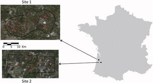
Two study sites were selected to investigate different parameters by introducing uncertainty related to forest attribute estimates derived from ALS data. Both forest sites are located in the Landes region in southwestern France (Figure 1). Site 1 (44.69° N, 0.90° W) and site 2 (44.40° N, 0.50° W) had surface areas of 80 km² and 60 km², respectively. The Landes forest is characterized by nutrient-poor sandy soil and a flat topography. Climate of the region is oceanic (Joly et al. 2010). The area is dominated by mono-specific stands of Maritime pine (Pinus pinaster Aiton) in even aged plantations. Some Pedunculate oaks (Quercus robur L.) are marginally present (∼1%). Both sites were highly representative of Landes forest diversity in terms of forest structure, and management practices.

Figure 1. Location of the 2 study sites in the Landes region, in southwestern France. Red dots represent field plot positions at both sites.

Field plot data

Field measurements were collected on a series of sample plots for each study site. A stratified random sampling design has been used to define field plot positions at both sites. The stratification was based on stand age (young, intermediate and mature stands). As recommended by Laes et al. (2011), for plots in a mixed condition, i.e. overlapping two or more stands, the plot centre was moved so the field measurements only represent a single condition. A different field protocol was used for each site. Hundred square plots (400 m²) were measured at site 1 during the summer of 2012 where all the trees were identified and their species recorded in order to assess the total tree number per plot. In addition, the DBH for the 10 trees closest to plot center and H of the 5 trees closest to plot center were measured. Thirty-nine circular plots were measured at site 2 during spring 2011. For plots having at least one tree with a DBH ≥ 17.5 cm, plot radius was set at 15 m (∼707 m², 31 plots). For plots with trees with all DBH under 17.5 cm, plot radius was set to 6 m (∼113 m², 8 plots). In these plots, all trees with DBH ≥ 7.5 cm were measured and, for each tree information were collected on their: (1) position in the plot, (2) species, (3) DBH, and (4) H.

Stand attributes measured in the field are summarized in Table 1 for both sites. The Gini coefficient was calculated from tree basal areas (BAs) for each plot in both sites. The Gini coefficient is used to measure tree size heterogeneity within a forest stand (Lexerød and Eid 2006). This index has a minimum value of zero, expressing perfect uniformity when all trees are of equal size. Unlike site 2 plots, site 1 plots include few very young seedling tree stands with much higher stem densities combined to low mean tree heights and low BAs (Table 1).

Table 1. Summary of stand attributes measured in the field for site 1 and 2; mean tree height, stem density, BA (Basal Area) and Gini coefficient were computed for each plot.

	Mean tree height (m)	Stem density (trees/ha)	Basal Area (m²/ha)	Gini coefficient
Site 1 (100 plots)
Min	2.2	150	0.4	0.06
Mean	13.6	950	24.2	0.23
Max	25.4	7150	54.3	0.45
Site 2 (39 plots)
Min	5	142	4.9	0.10
Mean	18.4	464	22.3	0.19
Max	29.5	1415	42.2	0.42

AGB is the dry mass (Mg/ha) of all the tree compartments that are above ground, including stems, branches, and leaves. AGB was estimated for each field plot. For trees with both H (m) and DBH (cm) measurements, individual tree AGB was derived from H and DBH using species-specific allometric equations. In site 1, for trees without height measurements, H was estimated from DBH using plot- or site-specific allometric relationships between H and DBH. In site 1 plots, for trees with neither H nor DBH measurements, AGB was extrapolated from the mean tree AGBs of the measured trees. Four allometric equations were available to estimate AGB for Maritime pine; the dominant species (see section 3.3.1-7) and, the allometric equation from Hounzandji et al. (2015) was used for Pedunculate oak. Estimations at plot level were then rescaled to per-hectare values. Using the allometric equation from Shaiek et al. (2011) for Maritime pine, mean plots AGBs were estimated at 71.8 Mg/ha in site 1 and 77.5 Mg/ha in site 2.

Lidar data

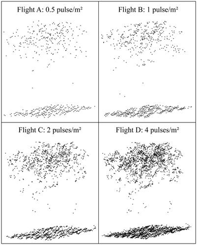
ALS data were collected at both study sites using a small footprint lidar. Site 1 was surveyed in February 2013 using an ALTM 3100 (Optech, Canada) system. Four different acquisitions were carried out with different flight parameters and system configurations in order to produce ALS data at different pulse density: (flight A) 0.5 pulse/m², (flight B) 1 pulse/m², (flight C) 2 pulses/m², and (flight D) 4 pulses/m². Site 2 was surveyed using a LMS Q560 (Riegl, Austria) system in April 2011 with a pulse density of 8 pulses/m². Additional data specifications for ALS data sets are given in Table 2. For both sites, lidar surveys were conducted at the same growing stage as field surveys.

Table 2. Technical specifications of lidar surveys on both study sites.

	Site 1				Site 2
	A	B	C	D
Date of survey	February 2013				April 2011
ALS sensor	Optech ALTM 3100				Riegl LMS Q560
Wavelength (nm)	1064				1550
Ground speed (m/s)	80				50
Beam divergence (mrad)	0.8				0.5
Maximum scan angle (°)	25	14	16	16	29.5
Repetition rate (Hz)	70	50	70	70	100
Flight altitude (m)	1530	2250	1530	1530	550
Pulse density (pulses/m²)	0.5	1.0	2.0	4.0	8.0

Data pre-processing was performed by the data providers, i.e. IGN and Sintegra for sites 1 and 2, respectively. Ground points were classified using the TIN-iterative algorithm (Axelsson 2000) in order to produce a digital terrain model (DTM). The DTM was then converted into a 1 m resolution grid. For each acquisition, aboveground heights were calculated by subtracting from each lidar point elevation the corresponding ground elevation given by the DTM, thereby removing topographic effects from lidar point clouds. From the resulting lidar point clouds, sub-point clouds corresponding to the spatial extent of each field plot were extracted.

Methods

We adopted an ABA and developed regression models for AGB predictions from lidar data according to a recent method developed by Bouvier et al. (2015, section 3.1). We selected only one methodology from among all those available as we wished to focus on the parameters explaining AGB prediction accuracy variability rather than model selection. We chose parameters that were easy to control when implementing an ABA approach, i.e. lidar pulse density and both field sampling protocols and measurements. Considering the available data sets, the following 8 parameters were studied: lidar pulse density, field plot number and size, minimum DBH threshold defining trees to be inventoried (DBHmin), H and DBH measurement errors, position accuracy of plot centers, and the choice of allometric equation. Two sensitivity analysis approaches were used to investigate the role of these parameters in the prediction quality of AGB models. The first was a standard OFAT approach. When this approach was applied, regression analyses were carried out to assess the influence of key parameters individually on AGB accuracy. Each parameter was tested using a wide range of values in order to assess its specific impact on AGB prediction accuracy. The parameter value ranges were defined by gradually degrading the characteristics of the available data sets (section 3.3) except in the cases of the choice of allometric equations (section 3.3.1-7) and pulse density (section 3.2). The second approach used was a GSA based on Monte Carlo simulations. This approach aimed at identifying the parameters related to field protocols and measurements that explain most AGB prediction variance and also interactions between parameters (section 3.4). Data processing was performed in the R statistical environment (R Core Team 2017). Lidar data were partly processed using the package ‘lidR’ (Roussel et al. 2018b) and the package ‘Sensitivity’ (Looss et al. 2018) was used for global sensitivity analyses.

Modeling approach

We used the method described by Bouvier et al. (2015), which was then used to produce AGB models from 4 categories of lidar metrics. This approach was tested and validated in several forest environments. The model is developed using 4 metrics to describe complementary 3D structural aspects of a stand unlike conventional statistical models that are based on height and point density distribution metrics (Næsset 2002). The 4 metrics were estimated from ALS data: mean canopy height (μ_CH); height heterogeneity (σ²_CH); horizontal canopy distribution (P); and a metric that was estimated from leaf area density profiles to provide information on stand vertical structure (Cv_LAD) was calculated as the average of first return heights. σ²_CH was calculated as the variance of first return heights. P was calculated from the lidar data as the ratio of the number of first returns below 2 m to the total number of first returns. Lastly Cv_LAD was calculated as the ratio of the standard deviation to the mean of the leaf area density profile. The density profile was computed by assessing a transmittance profile and then using the Beer-Lambert law to retrieve vegetation density at each height interval (Bouvier et al. 2015). μ_CH, σ²_CH, P and Cv_LAD were assessed considering only returns above 2 m for each of the point cloud subsets corresponding to the areas covered by each of the field plots. The metrics were included in a multiplicative power model with the coefficients fixed through a regression models based on these metrics.

In order to make an unbiased assessment of the predictive capacity of a model, a reference data set is generally created independently of the calibration or training data set (Snee 1977). Unfortunately, there were not enough training field plots to provide an independent validation data set. Therefore, the Leave-One-Out Cross-Validation (LOOCV) method, adapted to small data sets of less than 120 samples, was applied to evaluate the accuracy of the predictive models for both sites (Picard and Cook 1984; Martens and Dardenne 1998). This method was used to assess the goodness of fit of the model by averaging statistical estimators of model accuracy that were computed at each step of the cross-validation. The accuracy levels of AGB predictions were compared for diverse combinations of sampling parameters using 3 estimators: (1) the coefficient of determination (R²) was used to express the fraction of variance explained by the model; (2) the root mean square error (RMSE) as a representative measure of overall prediction quality; and (3) the prediction bias (bias). Unless otherwise stated, reference AGBs were computed using the allometric equation from Shaiek et al. (2011) for Maritime pine. For our study site, this equation was the only one found in the literature that explicitly estimates AGB from H and DBH measurements and that also covers a wide range of stand ages.

Influence of pulse density on the predictive performance of the model

Pulse density is an important parameter that significantly affects lidar point cloud characteristics (Figure 2). It is the most important and the only acquisition parameter included in this sensitivity analysis. Metric calculations may be influenced by a change in point cloud distribution. Thus, a decrease in pulse density may affect AGB prediction accuracy. We assessed and compared metrics and model results obtained in site 1 from ALS acquisitions for 4 pulse densities: 0.5, 1, 2, and 4 pulses/m², named flights A, B, C and D, respectively. To analyze the impact of pulse density on metrics, means and standard-deviations were computed for each metric and Student’s t-tests were performed to compare the mean of flight A metrics to the means of flights B, C and D metrics. Inter-metric correlations between lidar data sets for each of the 4 metrics were also computed.

Figure 2. A lidar point cloud acquired at 4 different pulse densities (0.5, 1, 2, and 4 pulses/m²) at site 1.

Influence of field data characteristics on the predictive performance of the model

A- Sensitivity analysis: One-factor-at-a-time (OAT)

Each parameter was varied within a range of values or choices in order to assess its effect on AGB prediction accuracy, while other parameters were set to their nominal value in the available field data sets. The ranges of values were defined by gradually degrading the characteristics of the data sets. Three parameters of the inventory protocol were first investigated: the number and size of field plots, and the DBHmin defining trees to be included in the database. Next, the accuracy of field plot measurements was also investigated considering respectively: H and DBH measurements, plot center positioning, and the choice of allometric equations used to predict reference AGB. For each studied parameter, evolutions in accuracy values were presented as a rate of change in RMSE considering the RMSE value obtained with the original and complete field data set. This reference RMSE changes depending on the site used to study the impact of each parameter.

Influence of the number of field plots

The more field plots, the higher prediction accuracy is likely to be. The optimal number of field plots is thus a trade-off between the quality of AGB predictions and the cost of field data acquisition. This optimal value also depends on field plot size, methodology used, and stand characteristics (Gobakken and Næsset 2009). Hundred field plots were collected in site 1, which made it possible to evaluate the influence of a lower numbers of field plots on model accuracy. Therefore, AGB was predicted using a subset of field plots from 100 to 20, in decrements of 1. Subsets were randomly selected among all field plots. A LOOCV method was applied to validate AGB predictions at each step. Subset selection was repeated 100 times leading to distributions of model accuracy measurements for each field plot number. Distribution characteristics according to field plot numbers were then compared.

Influence of the field plot size

The plot size chosen in most forest inventory programs is generally defined so as to optimize working time and reach accuracy requirements (Johnson and Hixon 1952). We investigated the importance of field plot size on site 2 for which trees were located within the plots, thus enabling to create new smaller plots by selecting trees using a criterion of distance from the plot center. Thirty field plots, which had a radius of 15 m, were used to predict AGB by decreasing plot radius from its maximum level at 15 m down to 6 m with regular steps of 0.5 m. The point cloud subsets were clipped accordingly to compute the metrics used to build and validate the models.

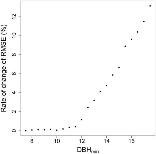
Influence of the minimum DBH threshold

Various DBHmin values have been used in forest inventories to determine if a tree should be included or not in the measurements made in the plot (Tomppo et al. 2010). We investigated impact of DBHmin on AGB prediction accuracy using the plots of site 2 where all trees with DBH ≥ 7.5 cm were collected. DBHmin ranged from 7.5 cm - value dictated by available field data - to 17.5 cm - maximum threshold value used in traditional field inventory (Duplat et al. 1981) - with a 0.5 cm step.

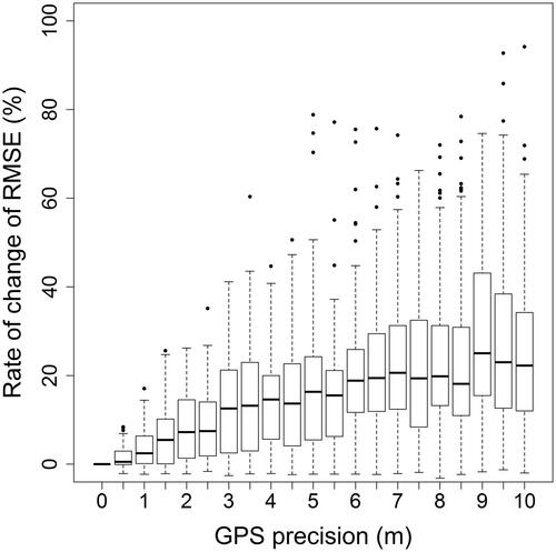
Influence of field plot position accuracy

The exact location of the field plot center is usually measured using differential GPS. Differential corrections are applied using the closest fixed antenna for position accuracy, which provide sub-meter accuracy. In forest applications, measurement accuracy can decrease because trees and terrain can obstruct clear views of the sky (Bolstad et al. 2005). In site 2, the GPS unit (Leica GPS 120, Switzerland) was placed in a forest clearing adjacent to the plot and away from dense cover. A total station (Leica TS02, Switzerland) was used to measure the exact distance to each plot center. Therefore, all field plots for site 2 had their central position estimated with less than 10 cm accuracy. The influence of plot central position accuracy on AGB predictions, and thus of a more or less important mismatch between field and ALS data, was evaluated by shifting field plot centers. For each simulated position, a new point cloud subset was clipped accordingly to compute the metrics used to build and validate the models. We tested position accuracy with error below 10 m. Two zero-mean Gaussian noises were added to the measured coordinates (x,y). σ ranged from 0 to 10 m with regular steps of 0.5 m. Error terms were assumed to be independent. Each step was repeated 100 times and the characteristics of the resulting AGB prediction model accuracy distributions were then compared.

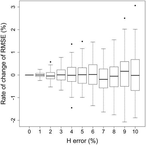
Influence of errors on the measurement of H

Multiple sources of error on AGB are linked to the measurement of H and DBH. These sources are dependent on the measurement method, stand characteristics, and the surveyor’s expertise (Kitahara et al. 2010; Larjavaara and Muller Landau 2013). In conifer stands, all conventional measurement methods produce errors ranging from 1% to 10% in H (Andersen et al. 2006). We investigated the influence of errors in H measurements on site 2 for which all trees with DBH ≥ 7.5 cm were inventoried. We assumed that measurement error was on average below 10%. H measurements were multiplied by a Gaussian noise centered on 1. Standard deviation σ was varied between 0 and 0.1 with regular steps of 0.01, corresponding to an error ranging from 0% to 10%. Each step was repeated 100 times independently of each other. The characteristics of the resulting AGB prediction model accuracy distributions were then compared.

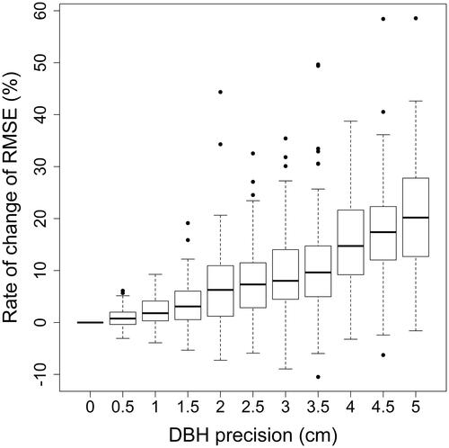
Influence of errors on DBH measurements

Error on measuring DBH was found to be 0.8 cm on average in temperate forests (Kaufmann and Schwyzer 2001). Measurement errors can even be higher for slanted trees, for trees with buttresses, or trees located on a steep slope. We investigated the influence of errors on DBH measurements for site 2 where all trees with DBH ≥ 7.5 cm were inventoried. We assumed that measurement error was on average lower than 5 cm for the DBH. Zero-mean Gaussian noises were added to the measured values of DBH. Standard deviation σ was varied between 0 and 5 cm with regular steps of 0.5 cm. Each step was repeated 100 times independently of each other. The characteristics of the resulting AGB prediction model accuracy distributions were then compared.

Influence of the selection of allometric equations

Allometric equations are commonly used to predict tree AGB. Plot AGB is estimated by the sum of the AGBs of all trees with a DBH above the chosen DBHmin. If inappropriate allometric equations are used for volume and tree AGB estimates substantial bias can result (Chave et al. 2004). We investigated the influence of several allometric equations on plot AGB prediction on site 2 for which all trees within the plots and with DBH ≥ 7.5 cm were collected. We focused on allometric equations for the Maritime pine, as it is by far the most dominant species (∼99% of all the trees in the inventory). Table 3 lists the sources of the allometric equations used. Equations 1, 2a and 2 b are explicitly AGB equations. Equations 2a and 2b were combined during the analysis to cover the whole range of stand ages observed in the study sites. Indeed, equation 2a was developed for smaller trees (1.5 < DBH < 16 cm) and equation 2b was developed for larger trees (29 < DBH < 52 cm). Equations 3 and 4 are total wood volume equations, including stumps and branches. A database providing expansion factors from total wood volume to AGB was used to predict the reference AGBs of plots in site 2 (Zanne et al. 2009). AGB prediction accuracy levels were compared when using the 4 allometric equations to obtain the reference data sets.

Table 3. Information summary on the 4 allometric equations used to predict reference AGB of the plots in Site 1.

	Reference	Attributes	Number of trees	Domain of validity
Equation 1	Shaiek et al. (2011)	DBH and H	178	5 < DBH < 48 cm
Equation 2a	Baldini et al. (1989)	DBH	8	1.5 < DBH < 16 cm
Equation 2b	Fraysse and Cotten (2008)	DBH	14	29 < DBH < 52 cm
Equation 3	Deleuze et al. (2013)	DBH and H	2145	7.6 < DBH < 79.3 cm
Equation 4	Dik (1984)	DBH and H	798	Not stated

These equations use DBH alone or both DBH and H to predict AGB. The number of trees used to calibrate these allometric equations is specified. Lastly, the DBH range relevant to apply each equation (the domain of validity) is specified.

B- Global sensitivity analysis (GSA)

A GSA was applied on site 2 (39 plots) to compare the relative effect of the studied parameters on AGB prediction variance and to identify possible interaction between parameters. The GSA method can be broken down into 3 steps. In the first step, the uncertainty of each studied parameter is modelled within a probabilistic framework, and a set of random combinations is sampled for each of them. In the second step of the GSA, uncertainty is propagated using pseudo-Monte Carlo simulations, repeatedly running AGB predictions using different sets of input parameters. A dedicated sampling scheme (Sobol′ 1974) is required to explore the space of uncertain parameters and to assess the resulting variance of AGB prediction. Contrary to the OAT analysis, all the parameters studied here are varied simultaneously, allowing us to capture the effect of inter-factor interactions. Finally, in the third and last step of the GSA, first-order variance-based sensitivity indices are estimated for each studied parameter, which are derived from the results of each model run. These sensitivity indices are based on the decomposition of the total output variance into conditional variances. First-order sensitivity indices measure the individual contribution of each uncertain parameter to the total variance of the AGB prediction. The remaining part of variance of the AGB prediction is explained by the inter-parameter interactions. The GSA approach was implemented in R, using sobol2007 function from the package ‘Sensitivity’. A detailed description of this Monte Carlo estimation of Sobol’ indices can be found in the references that are given in the reference manual of this package (Looss et al. 2018).

The influence of the 4 field parameters was explored for diverse inventory protocols. Accuracies related to field plot center position, H, and DBH and the choice of the allometric equation used to predict reference AGBs, were studied considering 4 different protocols depending on DBHmin (7.5 cm and 17.5 cm) and field plot size (radius of 11.28 m, i.e. a 400 m² plot, and 15 m, i.e. a 707 m² plot). For each protocol, we simulated field parameters n = 50,000 times, which led to a total of N = 300,000 combinations for each field plot (N=(n (k + 2)) with k the number of parameters under study (Saltelli et al. 2008)). The distribution laws to select values for H, DBH and plot position were defined as follows:

1. two zero-mean Gaussian noises were added to the measured coordinates (x,y) with a σ of 5 m which corresponds to a mean accuracy expected with a differential GPS in forest environments comparable to the Landes,

2. the measured H was multiplied by a Gaussian noise centered on 1 with a σ of 0.05 corresponding to a 5% error rate on H measurements, and

3. a zero-mean Gaussian noise with a σ of 1 cm was added to the measured DBH.

4. In addition, the allometric equation was selected randomly from among the 4 equations.

After each Monte Carlo run, AGB was predicted and compared to field reference. RMSEs were assessed at plot level and their distribution for each protocol compared. First-order and total indices obtained for the 4 inventory protocols were also compared.

Results

Influence of pulse density on the predictive performance of the model

Regression models were developed on site 1 for each acquisition, for varying pulse densities of 0.5, 1, 2 and 4 pulses/m². Metrics showed little sensitivity to changes in pulse densities (Table 4). Tests of mean equality were highly significant at the 0.05 level, with p-values ranging from 0.22 to 1.00. For each metric, correlations were also high between lidar data sets, with correlation coefficients ranging from 0.96 to 1 (Table 4). As a consequence, prediction accuracy barely improved with increasing pulse density. RMSE and RMSE% values ranged from 19.15 to 19.77 Mg/ha and from 26.7% to 27.5%, respectively, and only improved by a mere 3.1% when pulse density was increased by a factor of 8 (Table 5). Similarly, AGBs were predicted with a R² value of 0.86 when using the data set at a 0.5 pulse/m² while a R² value of 0.87 was obtained with the other data sets. Negative biases were found for all models, ranging from 5.75 to 6.20 Mg/ha.

Table 4. Impact of Lidar data pulse density on the 4 metrics (μ_CH, σ²_CH, P, Cv_LAD) used to build AGB models.

	Mean and standard deviation				Correlation (R)
	μ (± σ)
	p-values
Metric	Flight A	Flight B	Flight C	Flight D	Flights (A, B)	Flights (A, C)	Flights (A, D)	Flights (B, C)	Flights (B, D)	Flights (C, D)
	Reference
μCH	11.82	11.95	11.82	11.82	0.999	0.999	0.999	0.999	0.999	0.999
	(±5.99)	(± 6.01)	(± 6.00)	(± 6.00)
		p = 0.88	p = 1.00	p = 1.00
σ²CH	3.80	3.14	3.39	3.41	0.955	0.956	0.963	0.994	0.994	0.956
	(± 5.11)	(±4.23)	(±4.06)	(±4.17)
		p = 0.32	p = 0.54	p = 0.55
P	0.45	0.49	0.44	0.44	0.992	0.994	0.995	0.992	0.992	0.994
	(±0.25)	(±0.24)	(±0.25)	(±0.25)
		p = 0.26	p = 0.73	p = 0.66
CvLAD	2.03	2.17	2.08	2.07	0.983	0.977	0.973	0.988	0.988	0.977
	(±0.85)	(±0.87)	(±0.87)	(±0.88)
		p = 0.22	p = 0.67	p = 0.69

The metrics were computed for the 100 plots on site 1. Metric means (μ) and standard deviations (σ) are given for each lidar data set, as well as p-values of mean comparisons (reference values are Flight A metric means). Inter-metric correlations between lidar data sets for each of the 4 metrics are also given. Pulse densities are 0.5, 1, 2 and 4 pulses/m² for flight A, B, C and D, respectively.

Table 5. Goodness-of-fit for the 4 lidar acquisitions at site 1.

	R²	RMSE (Mg/ha)	RMSE%	Bias (Mg/ha)
Flight A (0.5 pulse/m²)	0.86	19.77	27.5	−5.75
Flight B (1 pulse/m²)	0.87	19.53	27.2	−6.20
Flight C (2 pulses/m²)	0.87	19.37	27.0	−6.09
Flight D (4 pulses/m²)	0.87	19.15	26.7	−5.87

For each data set, goodness-of-fit was expressed with 3 error estimators, R², RMSE, RMSE% and bias, and derived from the LOOCV (Leave-one-out-cross-validation).

Influence of field data characteristics on the predictive performance of the model

A- Sensitivity analysis: One-factor-at-a-time (OAT)

Influence of the number of field plots

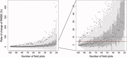
AGB was predicted using a constantly decreasing number of field plots from 100 to 20. The median rate of change of RMSE increased exponentially with the decrease in field plot number, giving rise to a low and quasi-linear increase in RMSE when number of field plots decreased from 100 to approximately 40 (Figure 3) and then to a sharp increase in mean RMSE. Median RMSE when using 20 field plots increased by around 53.1%, leading to RMSE and RMSE% values of 29.32 Mg/ha and 40.8%, respectively, when compared with AGB predicted using 100 field plots (i.e. RMSE = 19.15 Mg/ha and RMSE% = 26.7%). However, when using 40 and 60 field plots, the median RMSE increased by only about 10.4% (RMSE = 21.14 Mg/ha and RMSE%=29.4%) and 5.6% (RMSE = 20.22 Mg/ha and RMSE%=28.2%), respectively, when compared with AGB predicted using 100 field plots. The lower the field plot number, the higher the variability in model predictive performance. This was clearly observed with the interquartile ranges – calculated as the difference between the upper and the lower quartile values – which were 107.8%, 23.1%, and 13.2% respectively for 20, 40, and 60 field plots.

Figure 3. Rate of change of RMSE, expressed as a percentage of the RMSE obtained with the whole field plot data set, i.e. 19.15 Mg/ha with 100 plots, for AGB models calibrated and validated using different subsets of field plots from 100 to 20 at site 1. Subsets were randomly selected from among all the field plots and selection steps were repeated 100 times. Dark horizontal lines represent the median, with the box representing the 25th and 75th percentiles, the whiskers the 5th and 95th percentiles, and outliers are represented by dots. Two threshold values are also shown: an increase of 4.4% in RMSE (red line) leading to an AGB value of 20 Mg/ha (upper acceptable error for AGB predictions) and an increase of 10% in RMSE (gray line) leading to an AGB value of 21 Mg/ha.

Influence of field plot size

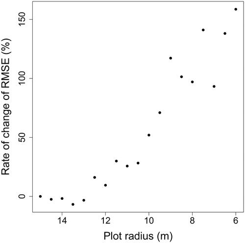
AGB was predicted from field plots of different radiuses ranging between 15 and 6 m. RMSE remained approximately constant as the plot radius was decreased from 15 to 13 m (Figure 4). Then RMSE increased linearly by 161.2% (RMSE = 28.03 Mg/ha and RMSE% = 36.2%) when the plot radius was decreased from 12.5 to 6 m, when compared with AGB predicted using a 15 m radius (i.e. RMSE = 10.73 Mg/ha and RMSE% = 13.8%).

Figure 4. Rate of change of RMSE, expressed as a percentage of the RMSEs obtained with the maximum plot radius, i.e. 10.73 Mg/ha with a 15 m radius, for AGB models calibrated and validated using different field plot radius from 15 to 6 m at site 2. Only the 31 plots collected in site 2 with radius of 15 m were used.

Influence of the minimum DBH threshold

AGB was predicted from field plots with different DBH_min. RMSE increased by only 0.4% when DBH_min increased from 7.5 to 11.5 cm (Figure 5). However, RMSE increased linearly by another 13.1% in relation to the reference RMSE and RMSE%, i.e. 10.73 Mg/ha and 13.8%, when DBH_min increased from 11.5 to 17.5 cm, leading to RMSE and RMSE% of 12.14 Mg/ha and 15.7%, respectively.

Figure 5. Rate of change in RMSE, expressed as a percentage of the RMSE obtained with DBHmin used in the field, i.e. 10.73 Mg/ha with DBHmin = 7.5 cm, for AGB models calibrated and validated using different minimum DBH thresholds (DBHmin) from 7.5 to 17.5 cm with regular steps of 0.5 cm. Only the 31 plots collected in site 2 with radius of 15 m were used.

Influence of field plot position accuracy

Compared to the reference RMSE of 10.73 Mg/ha and RMSE% of 13.8% obtained with the initial and accurate field plot center positions, median RMSE increased by 15.9% (RMSE = 12.44 Mg/ha, RMSE%=16.0%) and 22.3%, (RMSE = 13.12 Mg/ha, RMSE%=16.9%) when field plot centers were shifted by random error with standard deviation of 5 and 10 m, respectively (Figure 6). Variability in model predictive performance increased only slightly: the interquartile ranges were 9.5% and 10.9% with an error in field plot position of 5 and 10 m respectively.

Figure 6. Rate of change of RMSE, expressed as a percentage of the RMSE obtained with actual GPS precision obtained using both a DGPS and a total station, i.e. 10.73 Mg/ha for plot center position accuracy below 10 m, for AGB models calibrated and validated using field plots shifted by 2 random error terms (x,y) at site 2. Error terms were generated with standard deviation ranging from 0 to 10 m with regular steps of 0.5 m. Dark horizontal lines represent the median, with the box representing the 25th and 75th percentiles, the whiskers the 5th and 95th percentiles, and outliers represented by dots.

Influence of errors on the measurement of H

Changes in AGB prediction accuracy with increasing H measurement errors were observed and compared with the reference RMSE and RMSE% values obtained with actual H measurements, i.e. 10.73 Mg/ha and 13.8% (Figure 7). Median changes in RMSE remained close to zero, with variation ranging from 0.16% (RMSE = 10.75 Mg/ha and RMSE%=13.9%) to 0.10% (RMSE = 10.74 Mg/ha and RMSE%=13.9%) when the relative error on H measurement increased from 0% to 10%. However, variability in model predictive performance increased in step with increasing errors on H measurements. The interquartile ranges were 0.7%, and 1.4% with an error in H measurement of 5%, and 10%, respectively.

Figure 7. Rate of change of RMSE, expressed as a percentage of the RMSE obtained with actual H measurement values, i.e. 10.73 Mg/ha, for AGB models calibrated and validated using noisy H measurements at site 2. Error terms were generated with standard deviation ranging from 0 and 0.1 with regular steps of 0.01, corresponding to an error value ranging from 0% to 10%. Dark horizontal lines represent the median, with the box representing the 25th and 75th percentiles, the whiskers the 5th and 95th percentiles, and outliers represented by dots.

Influence of errors on DBH measurements

Changes in AGB prediction accuracy as a function of decreasing DBH precision were observed and compared with the reference RMSE and RMSE% values obtained with real DBH measurements, i.e. 10.73 Mg/ha and 13.8% (Figure 8). Median RMSE and RMSE% increased by 2.6% (RMSE = 11.01 Mg/ha and RMSE% = 14.2%) and 19.7% (RMSE = 12.84 Mg/ha and RMSE%=16.6%) when error terms added to the measured DBH values were set to 1 cm and 5 cm, respectively. Higher error on DBH measurements led to higher variability in model predictive performance. The interquartile ranges were 3.6%, and 15.1% for errors in DBH measurement of 1 and 5 cm respectively.

Figure 8. Rate of change of RMSE, expressed as a percentage of the RMSE obtained with real DBH measurement values, i.e. 10.73 Mg/ha, for AGB models calibrated and validated using noisy DBH measurements at site 2. Error terms were generated with standard deviation ranging from 0 to 5 cm with regular steps of 0.5 cm. Dark horizontal lines represent the median, with the box representing the 25th and 75th percentiles, the whiskers the 5th and 95th percentiles, and outliers represented by dots.

Influence of the selection of allometric equations

Using 4 independent allometric equations on site 2, predictions were assessed with R² values ranging from 0.93 to 0.95 and biases ranging from 1.56 to 1.93 Mg/ha (Table 6). For equations 1, 2 and 3, RMSE and RMSE% values range from 10.64 to 10.73 Mg/ha and from 13.7% to 13.8%, respectively. This represents a variation in RMSE of −0.84% and −0.65%, for equations 2 and 3 respectively when compared to RMSE obtained with equation 1, which is the reference value used for site 2. Equation 4 provided the highest RMSE value of 12.24 Mg/ha (RMSE% = 15.8%), i.e. a 14.07% increase in RMSE.

Table 6. Goodness-of-fit associated with the AGB predictive models using 4 allometric equations to predict reference AGB at site 2.

	R²	RMSE (Mg/ha)	RMSE%	Bias (Mg/ha)	Rate of change of RMSE (%)
Equation 1	0.94	10.73	13.8	−1.56	0
Equation 2	0.95	10.64	13.7	−1.71	−0.84
Equation 3	0.93	10.66	13.8	−1.87	−0.65
Equation 4	0.95	12.24	15.8	−1.93	14.07

Goodness-of-fit was expressed with 3 error estimators, R², RMSE, RMSE% and bias, and derived from the LOOCV (Leave-one-out-cross-validation). Rate of change of RMSE was expressed as a percentage of the RMSE obtained with the Equation 1, i.e. 10.73 Mg/ha.

B- Global sensitivity analysis

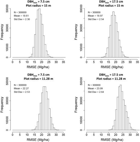
AGB values were predicted based on 300,000 combinations of the 4 studied factors, i.e. H, DBH, plot position and allometric equations, considering 4 field protocols defined according to both the field plot size and DBHmin for countable trees, i.e. either a 15 m or 11.28 m plot radius and 7.5 cm or 17.5 cm minimum DBH values. RMSE distributions were compared for the 4 field protocols in Figure 9. Not surprisingly, the highest AGB prediction accuracy value was observed when the smallest DBHmin of 7.5 cm and the largest field plot radius of 15 m were used, with a mean RMSE value of 18.61 Mg/ha (RMSE% = 24.0%) (Figure 9). RMSE was only slightly higher by 1.9% (18.97 Mg/ha (RMSE% = 24.5%)) with the same plot radius and a DBHmin of 17.5 cm. Lower AGB prediction accuracy value was obtained using a field plot radius of 11.28 m. RMSE values, which were 19.7% (22.27 Mg/ha (RMSE% = 28,7%)) and 28.1% (23.99 Mg/ha (RMSE% = 31.0%)) higher were found using a DBHmin it of 7.5 cm and 17.5 cm, respectively. The error value spread, depending on the field protocols used, also increased from 2.30 to 2.64 Mg/ha.

Figure 9. Histograms of RMSEs for the 300,000 Monte Carlo combinations obtained by varying H, DBH and field plot position measurement errors according to the defined distribution laws, and by varying the allometric equation used to predict AGB at site 2. Four protocols have been investigated: (a) 7.5 cm minimum DBH threshold (DBHmin) and 15 m field plot radius; (b) 17.5 cm DBHmin and 15 m field plot radius; (c) 7.5 cm DBHmin and 11.28 m field plot radius; and (d) 17.5 cm DBHmin and 11.28 m field plot radius.

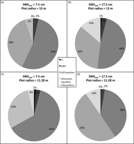
The part of variance attributable to each parameter, and linked to interactions between parameters, varied depending on which of the 4 inventory protocols was concerned (Figure 10). Whatever the inventory protocol, the part of variance explained by plot center positioning accuracy (38% – 63%) or the allometric equation used (29% – 50%) were significantly higher than the part of variance explained by the DBH (2% – 3%) and H (0% – 1%) parameters. In only one case – when the smallest DBHmin of 7.5 cm and the smallest field plot radius of 11.28 m were used – the part of variance explained by the allometric equation exceeded that explained by plot positioning accuracy (50% and 38%, respectively). The part of variance attributable to the interaction between parameters was found to be higher when the largest DBHmin (17.5 cm) and field plot radius (15 m) were used (14%), and also when the smallest DBHmin (7.5 cm) and field plot radius (11.28 m) were used (10%).

Figure 10. Part of variance explained by H, DBH and field plot position measurement errors, and allometric equations used to predict AGB at site 2. Four protocols have been investigated: (a) 7.5 cm minimum DBH threshold (DBHmin) and 15 m field plot radius; (b) 17.5 cm DBHmin and 15 m field plot radius; (c) 7.5 cm DBHmin and 11.28 m field plot radius; and (d) 17.5 cm DBHmin and 11.28 m field plot radius.

Discussion

Our goal was to identify the trade-offs that could be made on pulse density and field parameters that would not unduly compromise the predictive capabilities of ABA models using airborne lidar data. These trade-offs aim at reducing data acquisition costs as well as the resources required for field data collection while maintaining a sufficient level of model prediction capacity. Analyzing results derived from OAT sensitivity analysis and GSA helped to identify the relative impact of pulse density and field survey parameters therefore leading to concrete recommendations.

Pulse density is known to impact the value of some metrics at plot level (Gobakken and Næsset 2008). However, the 4 metrics used in our model were found to be weakly or insensitive to pulse density and prediction accuracy decrease of merely 3% (0.62 Mg/ha) was obtained for a pulse density decrease from 4 to 0.5 pulses/m². Our results confirmed those of Gobakken and Næsset (2008) and Treitz et al. (2012) for which lidar data obtained at a 0.5 pulse/m² density, or lower, did not affect significantly model predictability. There might be a critical threshold for pulse density below which AGB prediction accuracy would decrease significantly, as observed by Magnusson et al. (2007). However, we did not reach that threshold for the studied forest environment. A critical threshold value for pulse density under which AGB model prediction degrade significantly is an important consideration and may be tied to stand complexity. For operational surveys, conducting a specific sensitivity analysis prior to data acquisition is not conceivable. Pulse density should be set at the density level required for the most complex stand present in the surveyed area and based on results from the literature. This is why this issue is worth addressing in more depth in order to provide recommendations for a range of forest environments. For homogeneous pine plantations, lidar pulse densities can be reduced to 0.5 pulses/m² without any significant accuracy loss when predicting AGB with area-based approaches based on lidar metrics that are little sensitive or insensitive to pulse density. It is worth noting that this statement on pulse density does not apply to individual tree-based approaches that require several lidar measurements per tree crowns, hence at least a few points/m². In addition, optimal point density for tree-based approaches is likely to change according to stand type and age (Durrieu et al. 2015). Whereas 2 points/m² was found to be sufficient in mature stands, at least 10 points/m² might be required for saplings (Kaartinen et al. 2012).

In order to successfully use ALS data, the fieldwork required to provide the reference data sets needed to develop robust predictive models represents a significant share of the costs incurred (Eid et al. 2004). In this study, we distinguished 6 parameters related to field sampling protocols and measurement accuracies required to predict AGB, i.e. (1) the number of field plots, (2) field plot size, (3) DBHmin, (4) plot center position accuracy, (5) H measurement accuracy, (6) DBH measurement accuracy, and a seventh parameter, the allometric equation used. Critical thresholds were observed for several parameters.

First, we found that increasing the number of field plots used to predict AGB significantly increased the prediction accuracy up to about 40 or 50 field plots. For instance, AGB median prediction error was 50% higher for 20 field plots when compared to results obtained for 100 plots (Figure 3). Below 40 plots, it is not, for example, possible to capture forest stand variability and geographical trends related to silvicultural practices and site productivity. The upper acceptable error for AGB predictions is 20 Mg/ha or 20% of field estimates (whichever is greater and without exceeding errors of 50 Mg/ha for a global biomass map at 1 ha resolution) (Zolkos et al. 2013). In site 1, the mean AGB of the field plots was estimated at 71.8 Mg/ha. Twenty percent of this value equals to 14.4 Mg/ha, which is lower than 20 Mg/ha that can be used as a guideline for this site. In Figure 3 we can see that when the number of plots falls below 40, in addition to a faster rise in errors, first quartiles of RMSE distributions are no more systematically lower than 20 Mg/ha (red line in Figure 3) and median RMSEs systematically exceed 21 Mg/ha (grey line in Figure 3), which corresponds to an increase of 10% in the reference RMSE (i.e. 19.15 Mg/ha with 100 plots). RMSE distributions show that the risk of exceeding the acceptable errors for biomass prediction is high when the prediction models are developed with less than 40 plots.

Too few plots may also lead to significant overestimations in model accuracy as illustrated by the large spread in RMSE values. In our study, the increase in the distribution’s spread of rates of change of RMSE with the decrease in the number of plots was intensified by the random selection of plots among the initial plot set. Without stratification, some of the resulting samples could be composed of a set of plots that could either be highly unbalanced regarding the initial strata or gather a set of atypical plots. In such conditions, the predictive performance of the model is expected to be low. Conversely, the selected plots could by chance be an ‘ideal’ sample leading to a model with an apparent very good predictive performance but with a low generalization capacity. Applying plot selection strategies to ensure good representativeness of forest type heterogeneity lead to a decrease in the RMSE spread and an increase in the confidence level of the model (Maltamo et al. 2011). In their study, Maltamo et al. (2011) found that, when simulating a random sampling scheme (100 repetitions), the mean RMSE obtained for volume models was the same as the RMSE of models developed using a stratified random selection. In our study, the median value of the rates of change of RMSE can thus be considered to be a reliable indicator of the expected decrease in the predictive quality of the model if a stratified random sample design had been used. With a stratified sampling scheme, the confidence interval of this estimator is also expected to be significantly reduced compared to the one we obtained with random sampling. This point would deserve a specific analysis but, based on our study, we can state that, even in a relatively simple forest environment like the one studied here, 40 plots appear to be a minimum to build an AGB predictive model meeting user requirements. It has been also demonstrated that for complex forests, stratification improved model performance (Heurich and Thoma 2008; Bouvier et al. 2015), so a minimum number of 40 plots per strata should be advocated. This is quite high and can lead to excessive costs. The need to analyze how other field parameters can be relaxed without significantly degrading model results is all the more justified to counterbalance the minimum requirement in the number of field plots.

Second, when addressing field plot size issues, Gobakken and Næsset (2008) indicated that a lower number of required plots may be compensated through an increase in plot size. Unfortunately, we could not directly test this hypothesis with our data sets as we could not reduce both the plot radius and the number of field plots simultaneously. Indeed, plot radius could only be reduced in site 2, where each tree present has been located, but there are very few plots on this site. Nevertheless, we did observe an increase of approximately 160% in AGB prediction error when using a field plot radius of 6 m compared to 15 m (Figure 4). For our study site, we observed a critical threshold value of 13 m for field plot radius above which the larger plot radiuses did not significantly impact AGB prediction accuracy. This is consistent with the results obtained by Fassnacht et al. (2018) who reported that RMSE values of biomass predictions improved strongly for plot areas between 0.01 and 0.06 ha (equivalent to a fixed radius of 5.6 m and 14.1 m, respectively) then started to level out. It is worth noting that several countries use field plots with a diameter below 13 m for their forest inventory protocol (Tomppo et al. 2010).

Third, a critical value was found at 11.5 cm for the minimum DBH threshold. AGB prediction errors were lower by around 13% when compared with the DBHmin at 17.5 cm (Figure 5). Larger DBHmin degraded AGB prediction because lidar point clouds describe within a plot all the vegetation visible from above including the smallest trees. Site 2 is characterized by quite homogenous stands and the set of plots used was made up of plots with a 15 m radius mainly comprised of trees with a DBH greater than 17.5 cm. Therefore, this critical value is likely to be highly site and experiment dependant.

Fourth, the influence of field plot position accuracy on AGB predictions was also observed. Plot position accuracy requirements have an impact on costs because accurate positioning of plot centers may be time-consuming and require the use of expensive GPS receivers or even the use of both differential GPS and total stations. Error increased by around 16% and 22% when mean errors of 5 m and 10 m were respectively added to the GPS positioning measurement of the field plot center. In the worst cases the error level could even reach 94% (Figure 6). Extreme error values were probably linked to simulations for which several plots located close to a stand boundary were moved to a neighboring stand with different age and structure profiles. The impact of co-registration error might be significantly higher in more complex stands, which are characterized by heterogeneous stands and complex topography. In their study, McRoberts et al. (2018) concluded that using survey grade GPS receivers instead of field grade GPS receivers was not worth the high investment costs to equip field crews as they found that a lower location accuracy had effects of 5% or less on estimates of mean AGB per unit area and detrimental effects on standard errors of estimates of the mean on the order of 5–20%. However, in their analysis, the authors considered AGB estimations obtained with models built using plot locations from survey grade receiver as the reference and assumed that such receivers provide sub-metric location errors. This is probably optimistic and the real-location errors under forest covers are likely to be higher than 1 or 2 meters. For example, Piedallu and Gégout (2005) reported mean positioning errors of 1.6 m and 2.2 m in coppice and high forest stands, respectively, with a survey grade GPS and after differential correction was carried out. In our study we found a median increase in RMSE of about 10% when plot location accuracy degraded from less than 10 centimeters to 2 meters. In their study conducted in mixed boreal stands, Huang et al. (2013) also concluded that the use of DGPS with a best accuracy of 0.5–1.0 m for field measurements had contributed to the reliable biomass predictions they obtained at the level of LVIS footprints (R² = 0.86, RMSE = 31.0 Mg/ha, RMSE% = 25.1% with plots of 20 m diameter). This is why we are less categorical than McRoberts et al. (2018) and we would like to recommend that more studies are done on the impact of geolocation accuracy on biomass assessment as well as studies aiming at identifying measurement protocols for improved location accuracy in forest environments.

Fifthly, H measurement errors did not significantly impact AGB prediction accuracy for the studied range of errors, i.e. from 0% to 10% (Figure 7). Even the impact of the H error on the variability of RMSE estimations remained low, within −2 and +3% without considering outliers.

Sixthly, we found that DBH measurement errors had a significant impact on AGB prediction accuracy. Mean DBH errors of 5 cm were found to increase median AGB error by approximately 20% with high variability in RMSE estimations ranging from -3 to 43% (Figure 8). An allometric equation developed by Shaiek et al. (2011) has been used here to study H and DBH measurement errors. In this equation, H and DBH have different power values, i.e. 0.12 and 2.38, respectively. Power values may explain different impacts of measurement errors for both parameters on AGB prediction accuracy.

Overall, for the field parameters discussed above the number of field plots, field plot radius and plot center position accuracy appeared to be the most critical parameters when focusing on AGB prediction accuracy. Based on the results of OAT sensitivity analyses, we could identify critical threshold values under which, for field plot radius and DBHmin, or above which, for plot position accuracy, the performance of AGB prediction models is expected to decrease sharply and to become insufficient to meet forester needs. These values however are likely to be highly site dependent. In addition, in homogenous even-aged plantations, alleviating the field protocol by only measuring a sample of trees in the plots (e.g., like in the field protocol used in this study for site1, with only the 5 and 10 trees closest to plot center measured for H and DBH, respectively) can be done without a major impact on AGB prediction accuracy. Indeed, extrapolating AGB for non-measured trees can be equated to H and DBH measurement errors, which were found to be of minor importance compared to the other sources of error.

Selection of allometric AGB equations is known to significantly impact the accuracy of the reference AGB estimates (Chave et al. 2004; Duncanson et al. 2017). In this study, we observed maximum differences in AGB references assessed at plot level using the 4 allometric equations ranging from 5 to 66 Mg/ha. Allometric equations can impact prediction accuracy, through changes in the reference AGB values that are used to calibrate and validate the models. Results of the GSA reveal that a large part of the variance of AGB predictions can be attributed to the allometric equation used (from 34% to 50% of the total variance according to the field inventory protocol, i.e. plot radius and DBHmin used to select the measured trees). This underlines the importance of the choice of allometric equations on model results. Equation 1 is expected to provide the most accurate assessment of real AGB values because (1) it was built from measurements in the same geographic area, like all the other equations except equation 4, (2) it aims at assessing directly AGB unlike equations 3 and 4 that were built to assess wood volume that need to be further transformed to AGB using an expansion coefficient, and (3) it uses both H and DBH values, unlike equation 2, and was established using more trees than equation 2. The model built from reference AGB values obtained using equation 1 was thus used as the reference. Yet, when the 4 models built using the reference data sets obtained with the 4 allometric equations were compared, the metrics used to assess model performances were quite similar, except for the model based on AGB values computed with equation 4 with the highest RMSE (Table 6). RMSE increased by 15% between the lowest and the highest values obtained using the 4 selected allometric equations (Table 6). Equation 4 was the only allometric equation that was not calibrated using measurements from Maritime pines of the Landes forest. The lowest RMSE was obtained with the only allometric equation that used DBH measurements alone to predict AGB. This result suggests that the 4 lidar variables used as predictors may not completely describe the variability in AGB values, as values obtained with equation 1 are assumed to be the most accurate. Even-aged plantations, like those studied here, result in reduced competition between trees. For our study results, we thus obtain a stronger relationship between H and DBH and a higher correlation between these 2 explanatory variables (Chave et al. 2004). Therefore, using an allometric equation based on DBH values alone should provide, in this case, good AGB reference data. Also, such simplified equations represent an opportunity to develop models to predict AGB from lidar data for this forest type while reducing field measurement costs, and without any resulting loss in accuracy. Heterogeneous forest types may impose the selection of allometric equations using both DBH and H to capture intrinsic variability. RMSEs obtained using the 3 other equations are almost identical, but AGB predictions that result from the corresponding models are significantly different. In practice, there is always a limited number of allometric equations to choose from for a given species or group of species and it is very difficult to decide which equation provides the results closest to the truth. To improve biomass predictions there is a real need for improved allometric equations along with reliable validation information.

The relative importance of each parameter under study, except pulse density and plot number, was assessed based on a GSA analysis applied on site 2, that considered 4 field survey protocols (two plot radius – 15 m and 11.28 m – and 2 DBHmin – 7.5 cm and 17.5 cm) with standard forest inventory values regarding plot center position accuracy and both DBH and H measurement accuracies. When comparing results from the OAT and GSA (Figure 10) approaches, the same trend was observed: a decrease in field plot radius had a greater impact compared to an increase in the minimum DBH threshold value. GSA results also confirmed that errors in H and DBH measurements have respectively a negligible and minor impact, compared to plot center geolocation error and allometric equation. Based on findings from both approaches, the influence of parameters on AGB prediction accuracy can be ranked into 4 categories:

1. Main sources of error: field plot number, plot radius, plot center positioning accuracy,

2. Intermediate sources of error: allometric equations and DBHmin,

3. Minor sources of error: DBH measurement accuracy and pulse density, and

4. Negligible sources of error: H measurement accuracy.

The scope of this study was limited to: the impact of lidar pulse density, parameters related to field protocols and measurements, and of the choice of allometric equations. However, methods used to predict AGB from lidar data represent a further parameter affecting both quality and consistency of predictions (Hyyppä et al. 2008). AGB prediction accuracy also depends on stand complexity and homogeneity. Our study sites were composed of coniferous stands where measurements were easier to achieve and prone to less error when compared with deciduous stands. Therefore, the optimal combination of survey parameters may differ from one forest type to another. We recommend that future research concentrates on the influence of sampling design parameters depending on forest type.

Conclusion

We investigated the influence of sampling design parameters on AGB prediction accuracy from ALS data. Numerous parameters may impact the implementation of predictive models but only a few of them can be easily controlled. As impacts are generally inter-dependant and thus difficult to compare, the relative importance of parameters is difficult to assess. The influence of these key parameters was assessed individually by carrying out sensitivity analysis in order to define which parameter has the most influence on AGB prediction accuracy. Thus, using an OAT approach, we explored the impact of: pulse density, the number of field plots, field plot size, minimum DBH threshold, field plot position accuracy, H and DBH measurement accuracies, and allometric AGB equations. As some uncertainties can accumulate and propagate, the influence of field parameters was also investigated in a GSA.

Some recommendations can be drawn from our results for those interested in estimating AGB from a lidar-based ABA of mono-specific pine plantations. First, regarding ALS data acquisition, cost savings can be made by reducing pulse density to 0.5 pulse/m² without any major impact on model quality when using the model developed in Bouvier et al. (2015). Indeed, the 4 metrics used in this model were found to be very little sensitive or insensitive to pulse density for densities between 0.5 and 4 pulses/m², thus fostering model robustness. Even if H and DBH measurement accuracies were shown to contribute to a lesser extent to the prediction error, field measurement costs will still remain high to ensure a good-quality model. This is due to requirements regarding field plot number, position accuracy and plot size. Therefore, and despite the relative simplicity of the environment, a minimum of 40 plots is recommended. Plot positioning efforts should be performed with great care and position accuracy of center plots of below 5 m is highly recommended. It might be even more important to follow these recommendations when working in more complex forest environments, as the error related to plot positioning might be higher. In addition, it is also recommended to inventory field plots at least 13 m in radius when plots contain trees with a DBH equal or greater to 17.5 cm. Special attention should be paid to the choice of the allometric AGB equation.

Acknowledgements

We would like to thank the Institut National de l'Information Géographique et Forestière (IGN) for providing the lidar data set for site 1 and Laurent Albrech for his help during field campaign in site 2. We are also thankful to journal referees who made numerous helpful suggestions to improve of our manuscript.

Additional information

Funding

This research was supported by the French National Research Agency (ANR) Grant within the Framework of the FORESEE project [ANR 2010-BIOE-008]. The contribution to the development of the package « lidR » was partly supported by the GRAINE program of ADEME (Agence de l’Environnement et de la Maîtrise de l’Énergie) (PROTEST project [1703C0069]) and by ONF (convention TETIS-2015-227). The authors also wish to acknowledge the financial support of the governments of Quebec and France (Commission permanente de coopération franco-québécoise) through the Samuel-de-Champlain program [project 64.114] facilitating collaboration leading to this article.

References

- Andersen, H.-E., Reutebuch, S.E., and McGaughey, R.J. 2006. “A rigorous assessment of tree height measurements obtained using airborne lidar and conventional field methods.” Canadian Journal of Remote Sensing, Vol. 32(No. 5): pp. 355–366. doi:https://doi.org/10.5589/m06-030.
- Ascough Ii, J.C., Maier, H.R., Ravalico, J.K., and Strudley, M.W. 2008. “Future research challenges for incorporation of uncertainty in environmental and ecological decision-making.” Ecological Modelling, Vol. 219(No. 3–4): pp. 383–399. doi:https://doi.org/10.1016/j.ecolmodel.2008.07.015.
- Axelsson, P. 2000. “DEM generation from laser scanner data using adaptive TIN models.” International Archives of Photogrammetry and Remote Sensing, Vol. 33: pp. 111–118.
- Baldini, S., Berti, S., Cutini, A., Mannucci, M., Mercurio, R., and Spinelli, R. 1989. “Prove sperimentali di primo diradamento in un soprassuolo di pino marittimo (Pinus pinaster Ait.) originato da incendio: aspetti silvicolturali, di utilizzazione e caratteristiche della biomassa.” Annali Istituto Sperimentale Selvicoltura, Vol. 20: pp. 385–436.
- Bolstad, P., Jenks, A., Berkin, J., Horne, K., and Reading, W.H. 2005. “A comparison of autonomous, WAAS, Real-time, and post-processed Global Positioning Systems (GPS) accuracies in northern forests.” Northern Journal of Applied Forestry, Vol. 22(No. 1): pp. 5–11. doi:https://doi.org/10.1093/njaf/22.1.5.
- Bouvier, M., Durrieu, S., Fournier, R.A., and Renaud, J.-P. 2015. “Generalizing predictive models of forest inventory attributes using an area-based approach with airborne LiDAR data.” Remote Sensing of Environment, Vol. 156: pp. 322–334. doi:https://doi.org/10.1016/j.rse.2014.10.004.
- Brown, S., and Lugo, A.E. 1984. “Biomass of tropical forests: A new estimate based on forest volumes.” Science (New York, N.Y.).), Vol. 223(No. 4642): pp. 1290–1293. doi:https://doi.org/10.1126/science.223.4642.1290.
- Cariboni, J., Gatelli, D., Liska, R., and Saltelli, A. 2007. “The role of sensitivity analysis in ecological modelling.” Ecological Modelling, Vol. 203(No. 1–2): pp. 167–182. doi:https://doi.org/10.1016/j.ecolmodel.2005.10.045.
- Chave, J., Condit, R., Aguilar, S., Hernandez, A., Lao, S., and Perez, R. 2004. “Error propagation and scaling for tropical forest biomass estimates.” Philosophical Transactions of the Royal Society of London. Series B: Biological Sciences, Vol. 359(No. 1443): pp. 409–420. doi:https://doi.org/10.1098/rstb.2003.1425.
- Chen, Q., and McRoberts, R. 2016. Statewide mapping and estimation of vegetation aboveground biomass using airborne lidar, 2016 IEEE International Geoscience and Remote Sensing Symposium (IGARSS), 4442–4444.
- Corona, P., and Fattorini, L. 2008. “Area-based lidar-assisted estimation of forest standing volume.” Canadian Journal of Forest Research, Vol. 38(No. 11): pp. 2911–2916. doi:https://doi.org/10.1139/X08-122.
- CREM. 2009. Guidance on the development evaluation and application of environmental models (Technical Report). US Environmental Protection Agency. Available at http://www.epa.gov/crem/library/cred_guidance_0309.pdf
- Deleuze, C., Senga Kiessé, T., Renaud, J.-P., Morneau, F., Rivoire, M., Santenoise, P., Longuetaud, F., Mothe, F., Hervé, J.-C., and Bouvet, A. 2013. Rapport final EMERGE sur les modèles de volumes. Projet ANR- 08-BIOE-003, Programme BIOE 2008.
- Dik, E.J. 1984. “Estimating the wood volumes of standing trees in forestry practice.” Uitvoerig Verslag « De Dorschkamp » (Netherlands), Vol. 19: pp. 1–114.
- Duncanson, L., Huang, W., Johnson, K., Swatantran, A., McRoberts, R.E., and Dubayah, R. 2017. “Implications of allometric model selection for county-level biomass mapping.” Carbon Balance and Management, Vol. 12(No. 1): pp. 18. doi:https://doi.org/10.1186/s13021-017-0086-9.
- Duplat, P., Perrotte, G., France, O.N., and Des, F. 1981. Inventaire et estimation de l’accroissement des peuplements forestiers. Office National Des Forêts.
- Durrieu, S., Véga, C., Bouvier, M., Gosselin, F., Renaud, J.-P., and Saint-André, L. 2015. “Optical remote sensing of tree and stand heights.” In Remote Sensing Handbook Vol II: Land Resources Monitoring, Modeling, and Mapping with Remote Sensing, edited by Prasad S. Thenkabail, Chapter: 17, 449–485. Boca Raton: CRC Press - Taylor & Francis Group.
- Eid, T., Gobakken, T., and Næsset, E. 2004. “Comparing stand inventories for large areas based on photo-interpretation and laser scanning by means of cost-plus-loss analyses.” Scandinavian Journal of Forest Research, Vol. 19(No. 6): pp. 512–523. doi:https://doi.org/10.1080/02827580410019463.
- Ene, L.T., Næsset, E., and Gobakken, T. 2016. “Simulation-based assessment of sampling strategies for large-area biomass estimation using wall-to-wall and partial coverage airborne laser scanning surveys.” Remote Sensing of Environment, Vol. 176: pp. 328–340. doi:https://doi.org/10.1016/j.rse.2016.01.025.
- European Commission. 2009. Impact Assessment Guidelines (p. 92). SEC.
- Fang, J.Y., Liu, G.H., and Xu, S.L. 1996. “Biomass and net production of forest vegetation in China.” Acta Ecologica Sinica, Vol. 16: pp. 497–508. doi:https://doi.org/10.1016/j.chnaes.2015.03.001.
- Fassnacht, F.E., Latifi, H., and Hartig, F. 2018. “Using synthetic data to evaluate the benefits of large field plots for forest biomass estimation with LiDAR.” Remote Sensing of Environment, Vol. 213: pp. 115–128. doi:https://doi.org/10.1016/j.rse.2018.05.007.
- Fraysse, J., and Cotten, L. 2008. Gestion de la fertilisation en fonction de l’exportation de biomasse. Sylvogene project, final report, 116–145.
- Frazer, G.W., Magnussen, S., Wulder, M.A., and Niemann, K.O. 2011. “Simulated impact of sample plot size and co-registration error on the accuracy and uncertainty of LiDAR-derived estimates of forest stand biomass.” Remote Sensing of Environment, Vol. 115(No. 2): pp. 636–649. doi:https://doi.org/10.1016/j.rse.2010.10.008.
- Gobakken, T., and Næsset, E. 2008. “Assessing effects of laser point density, ground sampling intensity, and field sample plot size on biophysical stand properties derived from airborne laser scanner data.” Canadian Journal of Forest Research, Vol. 38(No. 5): pp. 1095–1109. doi:https://doi.org/10.1139/X07-219.
- Gobakken, T., and Næsset, E. 2009. “Assessing effects of positioning errors and sample plot size on biophysical stand properties derived from airborne laser scanner data.” Canadian Journal of Forest Research, Vol. 39(No. 5): pp. 1036–1052. doi:https://doi.org/10.1139/X09-025.
- Goetz, S., and Dubayah, R. 2011. “Advances in remote sensing technology and implications for measuring and monitoring forest carbon stocks and change.” Carbon Management, Vol. 2(No. 3): pp. 231–244. doi:https://doi.org/10.4155/cmt.11.18.
- Hawbaker, T.J., Keuler, N.S., Lesak, A.A., Gobakken, T., Contrucci, K., and Radeloff, V.C. 2009. “Improved estimates of forest vegetation structure and biomass with a LiDAR‐optimized sampling design.” Journal of Geophysical Research: Biogeosciences, Vol. 114 (NO. G2):doi:https://doi.org/10.1029/2008JG000870.
- Heurich, M., and Thoma, F. 2008. “Estimation of forestry stand parameters using laser scanning data in temperate, structurally rich natural European beech (Fagus sylvatica) and Norway spruce (Picea abies) forests.” Forestry, Vol. 81(No. 5): pp. 645–661. doi:https://doi.org/10.1093/forestry/cpn038.
- Holmgren, J., Nilsson, M., and Olsson, H. 2003. “Simulating the effects of lidar scanning angle for estimation of mean tree height and canopy closure.” Canadian Journal of Remote Sensing, Vol. 29(No. 5): pp. 623–632. doi:https://doi.org/10.5589/m03-030.
- Hounzandji, A., Jonard, M., Nys, C., Saint-André, L., and Ponette, Q. 2015. “Improving the robustness of biomass function: from empirical to functional approaches.” Annals of Forest Science, Vol. 72(No. 6): pp. 795–810. doi:https://doi.org/10.1007/s13595-014-0423-z.
- Huang, W., Sun, G., Dubayah, R., Cook, B., Montesano, P., Ni, W., and Zhang, Z. 2013. “Mapping biomass change after forest disturbance: Applying LiDAR footprint-derived models at key map scales.” Remote Sensing of Environment, Vol. 134: pp. 319–332. doi:https://doi.org/10.1016/j.rse.2013.03.017.
- Hyyppä, J., Hyyppä, H., Leckie, D., Gougeon, F., Yu, X., and Maltamo, M. 2008. “Review of methods of small‐footprint airborne laser scanning for extracting forest inventory data in boreal forests.” International Journal of Remote Sensing, Vol. 29(No. 5): pp. 1339–1366. doi:https://doi.org/10.1080/01431160701736489.
- Johnson, F.A., and Hixon, H.J. 1952. “The most efficient size and shape of plot to use for cruising in old-growth Douglas-fir timber.” Journal of Forestry, Vol. 50: pp. 17–20.
- Joly, D., Brossard, T., Cardot, H., Cavailhes, J., Hilal, M., and Wavresky, P. 2010. “Les types de climats en France, une construction spatiale.” Cybergeo: European Journal of Geography. http://journals.openedition.org/cybergeo/23155, doi:https://doi.org/10.4000/cybergeo.23155.
- Junttila, V., Maltamo, M., and Kauranne, T. 2008. “Sparse Bayesian estimation of forest stand characteristics from airborne laser scanning.” Forest Science, Vol. 54: pp. 543–552.
- Kaartinen, H., Hyyppä, J., Yu, X., Vastaranta, M., Hyyppä, H., Kukko, A., Holopainen, M., Heipke, C., et al. 2012. “An international comparison of individual tree detection and extraction using airborne laser scanning.” Remote Sensing, Vol. 4(No. 4): pp. 950–974. doi:https://doi.org/10.3390/rs4040950.
- Kaufmann, E., and Schwyzer, A. 2001. Control survey of the terrestrial inventory. Swiss National Forest Inventory: methods and Models of the Second Assessment, edited by P. Brassel and H. Lischke, 114–124. Birmensdorf: WSL Swiss Federal Research Institute.
- Kitahara, F., Mizoue, N., and Yoshida, S. 2010. “Effects of training for inexperienced surveyors on data quality of tree diameter and height measurements.” Silva Fennica, Vol. 44(No. 4): pp. 657–667. doi:https://doi.org/10.14214/sf.133.
- Korhonen, L., Korpela, I., Heiskanen, J., and Maltamo, M. 2011. “Airborne discrete-return LIDAR data in the estimation of vertical canopy cover, angular canopy closure and leaf area index.” Remote Sensing of Environment, Vol. 115(No. 4): pp. 1065–1080. doi:https://doi.org/10.1016/j.rse.2010.12.011.
- Laes, D., Reutebuch, S.E., McGaughey, R.J., and Mitchell, B. 2011. “Guidelines to estimate forest inventory parameters from lidar and field plot - Companion document to the Advanced lidar applications - Forest inventory modeling class.” Vol. 22.
- Larjavaara, M., and Muller Landau, H.C. 2013. “Measuring tree height: a quantitative comparison of two common field methods in a moist tropical forest.” Methods in Ecology and Evolution, Vol. 4(No. 9): pp. 793–801. doi:https://doi.org/10.1111/2041-210X.12071.
- Lefsky, M.A., Harding, D., Cohen, W.B., Parker, G.G., and Shugart, H.H. 1999. “Surface lidar remote sensing of basal area and biomass in deciduous forests of eastern Maryland, USA.” Remote Sensing of Environment, Vol. 67(No. 1): pp. 83–98. doi:https://doi.org/10.1016/S0034-4257(98)00071-6.
- Lexerød, N.L., and Eid, T. 2006. “An evaluation of different diameter diversity indices based on criteria related to forest management planning.” Forest Ecology and Management, Vol. 222(No. 1–3): pp. 17–28. doi:https://doi.org/10.1016/j.foreco.2005.10.046.
- Li, Y., Andersen, H.-E., and McGaughey, R. 2008. “A comparison of statistical methods for estimating forest biomass from light detection and ranging data.” Western Journal of Applied Forestry, Vol. 23(No. 4): pp. 223–231. doi:https://doi.org/10.1093/wjaf/23.4.223.
- Lim, K., Treitz, P., Baldwin, K., Morrison, I., and Green, J. 2003. “Lidar remote sensing of biophysical properties of tolerant northern hardwood forests.” Canadian Journal of Remote Sensing, Vol. 29(No. 5): pp. 658–678. doi:https://doi.org/10.5589/m03-025.
- Looss, B., Janon, A., and Pujol, G. 2018. Sensitivity: Global Sensitivity Analysis of Model Outputs. R package version 1.15.2. https://CRAN.R-project.org/package=sensitivity
- Magnussen, S., Nord-Larsen, T., and Riis-Nielsen, T. 2018. “Lidar supported estimators of wood volume and aboveground biomass from the Danish national forest inventory (2012–2016).” Remote Sensing of Environment, Vol. 211: pp. 146–153. doi:https://doi.org/10.1016/j.rse.2018.04.015.
- Magnusson, M., Fransson, J.E., and Holmgren, J. 2007. “Effects on estimation accuracy of forest variables using different pulse density of laser data.” Forest Science, Vol. 53: pp. 619–626.
- Maltamo, M., Bollandsas, O.M., Næsset, E., Gobakken, T., and Packalen, P. 2011. “Different plot selection strategies for field training data in ALS-assisted forest inventory.” Forestry, Vol. 84(No. 1): pp. 23–31. doi:https://doi.org/10.1093/forestry/cpq039.
- Maltamo, M., Eerikäinen, K., Packalén, P., and Hyyppä, J. 2006. “Estimation of stem volume using laser scanning-based canopy height metrics.” Forestry: An International Journal of Forest Research, Vol. 79(No. 2): pp. 217–229. doi:https://doi.org/10.1093/forestry/cpl007.
- Martens, H.A., and Dardenne, P. 1998. “Validation and verification of regression in small data sets.” Chemometrics and Intelligent Laboratory Systems, Vol. 44(No. 1–2): pp. 99–121. doi:https://doi.org/10.1016/S0169-7439(98)00167-1.
- McRoberts, R.E., Chen, Q., Walters, B.F., and Kaisershot, D.J. 2018. “The effects of global positioning system receiver accuracy on airborne laser scanning-assisted estimates of aboveground biomass.” Remote Sensing of Environment, Vol. 207: pp. 42–49. doi:https://doi.org/10.1016/j.rse.2017.09.036.
- Næsset, E. 1997. “Determination of mean tree height of forest stands using airborne laser scanner data.” ISPRS Journal of Photogrammetry and Remote Sensing, Vol. 52(No. 2): pp. 49–56. doi:https://doi.org/10.1016/S0924-2716(97)83000-6.
- Næsset, E. 2002. “Predicting forest stand characteristics with airborne scanning laser using a practical two-stage procedure and field data.” Remote Sensing of Environment, Vol. 80(No. 1): pp. 88–99. doi:https://doi.org/10.1016/S0034-4257(01)00290-5.
- Næsset, E. 2004. “Practical large-scale forest stand inventory using a small-footprint airborne scanning laser.” Scandinavian Journal of Forest Research, Vol. 19(No. 2): pp. 164–179. doi:https://doi.org/10.1080/02827580310019257.
- Næsset, E. 2009. “Effects of different sensors, flying altitudes, and pulse repetition frequencies on forest canopy metrics and biophysical stand properties derived from small-footprint airborne laser data.” Remote Sensing of Environment, Vol. 113(No. 1): pp. 148–159. doi:https://doi.org/10.1016/j.rse.2008.09.001.
- Næsset, E., Bollandsås, O.M., and Gobakken, T. 2005. “Comparing regression methods in estimation of biophysical properties of forest stands from two different inventories using laser scanner data.” Remote Sensing of Environment, Vol. 94(No. 4): pp. 541–553. doi:https://doi.org/10.1016/j.rse.2004.11.010.
- Nelson, R., Krabill, W., and Tonelli, J. 1988. “Estimating forest biomass and volume using airborne laser data.” Remote Sensing of Environment, Vol. 24(No. 2): pp. 247–267. doi:https://doi.org/10.1016/0034-4257(88)90028-4.
- Nilsson, M., Nordkvist, K., Jonzén, J., Lindgren, N., Axensten, P., Wallerman, J., Egberth, M., et al. 2017. “A nationwide forest attribute map of Sweden predicted using airborne laser scanning data and field data from the National Forest Inventory.” Remote Sensing of Environment, Vol. 194: pp. 447–454. doi:https://doi.org/10.1016/j.rse.2016.10.022.
- Picard, R.R., and Cook, R.D. 1984. “Cross-validation of regression models.” Journal of the American Statistical Association, Vol. 79(No. 387): pp. 575–583. doi:https://doi.org/10.2307/2288403.
- Piedallu, C., and Gégout, J.C. 2005. “Effects of forest environment and survey protocol on GPS accuracy.” Photogrammetric Engineering & Remote Sensing, Vol. 71(No. 9): pp. 1071–1078. doi:https://doi.org/10.14358/PERS.71.9.1071.
- Roussel, J.R., Béland, M., Caspersen, J., and Achim, A. 2018a. “A mathematical framework to describe the effect of beam incidence angle on metrics derived from airborne LiDAR: The case of forest canopies approaching turbid medium behaviour.” Remote sensing of environment, Vol. 209: pp. 824–834.
- Roussel, J.-R., Auty, D., De Boissieu, F., and Sánchez Meador, A. 2018b. lidR: Airborne LiDAR Data Manipulations and Visualisation for Forestry Applications. R package version 1.6.0, https://github.com/JeanRomain/lidR
- R Core Team. 2017. R: A language and environment for statistical computing. R Foundation for Statistical Computing, Vienna, Austria. https://www.R-project.org/.
- Saltelli, A., Ratto, M., Andres, T., Campolongo, F., Cariboni, J., Gatelli, D., Saisana, M., and Tarantola, S. 2008. Global Sensitivity Analysis: the Primer. New-York: John Wiley & Sons.
- Shaiek, O., Loustau, D., Trichet, P., Meredieu, C., Bachtobji, B., Garchi, S., and Aouni, M.H. 2011. “Generalized biomass equations for the main aboveground biomass components of maritime pine across contrasting environments.” Annals of Forest Science, Vol. 68(No. 3): pp. 443–452. doi:https://doi.org/10.1007/s13595-011-0044-8.
- Snee, R.D. 1977. “Validation of regression models: methods and examples.” Technometrics, Vol. 19(No. 4): pp. 415–428. doi:https://doi.org/10.2307/1267881.
- Sobol′, I. M. 1974. The Monte Carlo Method. Popular Lectures in Mathematics, 72. Chicago, IL: The University of Chicago Press. (Order No. 767493; ERIC Number: ED184845).
- Strunk, J., Temesgen, H., Andersen, H.-E., Flewelling, J.P., and Madsen, L. 2012. “Effects of lidar pulse density and sample size on a model-assisted approach to estimate forest inventory variables.” Canadian Journal of Remote Sensing, Vol. 38(No. 5): pp. 644–654. doi:https://doi.org/10.5589/m12-052.
- Tarantola, S., Giglioli, N., Jesinghaus, J., and Saltelli, A. 2002. “Can global sensitivity analysis steer the implementation of models for environmental assessments and decision-making?.” Stochastic Environmental Research and Risk Assessment (Serra), Vol. 16(No. 1): pp. 63–76. doi:https://doi.org/10.1007/s00477-001-0085-x.
- Tomppo, E., Gschwantner, M., Lawrence, M., and McRoberts, R. E. 2010. National Forest Inventories. Pathways for Common Reporting. European Science Foundation.
- Treitz, P., Lim, K., Woods, M., Pitt, D., Nesbitt, D., and Etheridge, D. 2012. “LiDAR sampling density for forest resource inventories in Ontario, Canada.” Remote Sensing, Vol. 4(No. 4): pp. 830–848. doi:https://doi.org/10.3390/rs4040830.
- White, J.C., Wulder, M.A., Varhola, A., Vastaranta, M., Coops, N.C., Cook, B.D., Pitt, D., and Woods, M. 2013. “A best practices guide for generating forest inventory attributes from airborne laser scanning data using an area-based approach.” The Forestry Chronicle, Vol. 89(No. 6): pp. 722–723. doi:https://doi.org/10.5558/tfc2013-132.
- Woods, M., Pitt, D., Penner, M., Lim, K., Nesbitt, D., Etheridge, D., and Treitz, P. 2011. “Operational implementation of a LiDAR inventory in Boreal Ontario.” The Forestry Chronicle, Vol. 87(No. 4): pp. 512–528. doi:https://doi.org/10.5558/tfc2011-050.
- Young, M. 2000. Optics and Lasers: Including Fibers and Optical Waveguides (Vol. 5). Berlin: Springer.
- Zanne, A. E., Lopez-Gonzalez, G., Coomes, D. A., Ilic, J., Jansen, S., Lewis, S. L., Miller, R. B., Swenson, N. G., Wiemann, M. C., and Chave, J. 2009. Global wood density database. Dryad. Identifier: http://hdl.handle.net/10255/dryad, 235.
- Zolkos, S.G., Goetz, S.J., and Dubayah, R. 2013. “A meta-analysis of terrestrial aboveground biomass estimation using lidar remote sensing.” Remote Sensing of Environment, Vol. 128: pp. 289–298. doi:https://doi.org/10.1016/j.rse.2012.10.017.