Synthetic magnetotelluric modelling of a regional fault network – implications for survey design and interpretation

Abstract

The magnetotelluric (MT) method is increasingly being applied to mineral exploration under cover with several case studies showing that mineral systems can be imaged from the lower crust to the near surface. Driven by this success, the Australian Lithospheric Architecture Magnetotelluric Project (AusLAMP) is delivering long-period data on a 0.5° grid across Australia, and derived continental scale resistivity models that are helping to drive investment in mineral exploration in frontier areas. Part of this investment includes higher-resolution broadband MT surveys to enhance the resolution of features of interest and improve targeting. To help gain best value for this investment it is important to understand the ability and limitations of MT to resolve features on different scales. Here we present synthetic modelling of continuous, narrow, near-vertical faults 500 m to 1500 m wide with a resistivity 100–200 times less than the background rock resistivity using the ModEM software, and show that for such a situation a station spacing of around 14 km across strike is sufficient to resolve these into the upper crust. However, the vertical extent of these features is not well constrained, with near-vertical planar features commonly resolved as two separate features. This highlights the need for careful interpretation of anomalies in MT inversion. In particular, in an exploration scenario, it is important to consider that a lack of interconnectivity between a lower crustal/upper mantle conductor and conductors higher up in the crust and the surface might be apparent only, and may not necessarily reflect reduced mineral prospectivity.

KEYWORDS:

• Magnetotellurics
• fault
• mineral system
• inversion
• AusLAMP
• synthetic modelling

Introduction

In recent years, the magnetotelluric (MT) method has been shown to be effective in imaging mineral systems, particularly beneath sedimentary basin cover. Some mineral systems have been imaged from the lower crust and upper mantle to the deposit scale (Heinson et al. 2018; Wang, Duan, and Simpson 2018). This success has stimulated investment in the Australian Lithospheric Architecture Magnetotelluric Program (AusLAMP), which aims to deliver long-period MT data on a 0.5° grid across Australia (Duan et al. 2016, 2020, 2021; Duan and Kyi 2018; Kirkby et al. 2020; Kyi et al. 2020; Robertson, Thiel, and Heinson 2018; Thiel et al. 2016, 2020). Two goals of AusLAMP are to image Australia’s large-scale lithospheric architecture, and to identify new large-scale mineral system footprints, the understanding of which can be improved through a process of scale reduction that includes infill broadband MT.

Due to the rapidly increasing coverage, AusLAMP models have already identified many conductive anomalies in the middle to lower crust and upper mantle, several of which are of interest from a mineral exploration perspective (e.g. Duan et al. 2020, 2021; Kirkby et al. 2020; Robertson, Heinson, and Thiel 2016; Robertson, Thiel and Heinson 2018; Thiel et al. 2016, 2020). In order to understand if and how these anomalies connect to the surface, and to guide mineral exploration associated with these anomalies, higher-resolution surveys can be carried out using higher-frequency MT data to image the (shallow) crustal expression of these anomalies (e.g. Jiang et al. 2022). In order to obtain best value for investment in this higher-resolution data, it is important to be guided by an understanding of the trade-offs between site spacing and model grid resolution in terms of their ability to resolve important structures. Such an understanding can be gained through synthetic modelling where we can pre-determine the subsurface structure and learn how well it can be resolved in an MT inversion. In a real world scenario with finite budget, these considerations may also have to be balanced with the survey dimensions (i.e. area that can be covered) and the geological situation.

In this paper, we present synthetic modelling of a set of narrow, mainly trans-crustal fault zones of different orientation and dip which could represent a conductive fluid pathway architecture associated with a mineral system. While a main aim of our contribution is to illustrate the approach and to lay the foundation for follow-up studies, the size and design of our model resemble a regional-scale situation as, for example, presented in the follow-up interpretation of an AusLAMP resistivity model (e.g. Jiang et al. 2022). The main scientific aims of such a survey would be to image the resistivity architecture at crustal scale and to define the position and geometry of structures/conductors in the upper crust as close to the surface as possible. This then allows for integration with other datasets such as potential field data, geology, reflection seismic and airborne electromagnetics. We test multiple survey and model mesh designs to assess the ability of these to resolve the different fault zones in our hypothetical survey.

Method

Model setup

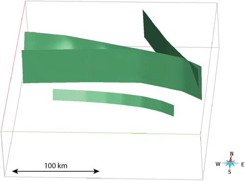
We construct a geological model containing four faults (Figure 1). The central two faults originate at 40 km depth with an approximately east–west strike, and have an east–west extent of around 200 km. They diverge such that they are ∼25 km apart near the surface, and have dips of 80° and 45°, respectively, to the south. Another north-northwest – south-southeast fault is splaying from the easternmost part of these faults, which is crustal scale and near vertical. We also add an east–west striking fault to the south, which is disconnected from the other faults and represents an isolated, upper crustal feature extending from the surface to a depth of 10 km. The geological model was digitised onto a model grid with two resolutions: 750 m (Scenario 1) and 500 m (Scenario 2). As a result, the faults are 750–1500 m (Scenario 1) or 500–1000 m (Scenario 2) wide. This setup represents an approximation of a real-world fault zone which might be expected to vary in thickness along its strike length and depth extent, however it provides a good basis to understanding how well structures like this can be imaged, and resolved, in magnetotelluric surveys of different resolutions. The width range used in this model is consistent with widths of major fault zones mapped in outcrop and in drillholes (Bourlange et al. 2003; Celestino et al. 2020; Choi et al. 2016; Morrow, Lockner, and Hickman 2015), and imaged in deep seismic reflection surveys (e.g. Calvert and Doublier 2018; Korsch and Doublier 2016).

Figure 1. 3D perspective view of the fault model used for synthetic inversion. Faults are shown in green. Diagram is shown on an equal horizontal and vertical scale.

The resistivity of the faults was set to 5 ohm-m (Scenario 1) and 10 ohm-m (Scenario 2) to represent two different scenarios: (1) a more conductive, thicker/wider fault zone, and (2) and more resistive, thinner/narrower fault zone (Figure 2). The resistivity values were selected to represent a fault zone either filled with a clay gouge (5-100 Ωm; Palacky 1988) or mineralised with conductive materials such as sulphides, magnetite or graphite, the resistivities of which are normally ≪ 1 Ωm and can be as low as 10⁻³ Ωm (Palacky 1988; Pearce, Pattrick, and Vaughan 2006; Vella and Emerson 2012). Thus, if interconnected, ∼0.02–20% (Scenario 1) or ∼0.01–10% (Scenario 2) of either, or a combination of these minerals in a rock with high resistivity (e.g. ≥ 1000 Ωm) would produce these resistivities. The resistivity range (5-10 Ωm) is consistent with resistivities measured across many fault zones across the world (e.g. Chiang et al. 2008; Morrow, Lockner, and Hickman 2015). In some cases, measured resistivity in fault zones is much less, e.g. 0.5–1.5 Ωm (Bourlange et al. 2003; Moore et al. 1995).

Figure 2. Synthetic model setup for calculating the forward responses, at 2 and 20 km depth. (a–b) example with a thicker, more conductive fault (750 m model cell size, Scenario 1), (c–d) example with a thinner, less conductive fault (500 m model cell size, Scenario 2). Black circles indicate sites on a ∼55 km grid, crosses indicate sites added for a ∼28 km densification around the faults, plus symbols indicate sites added for a ∼14 km densification in a N-S direction, and dots indicate sites added for a ∼7 km densification in a N-S direction.

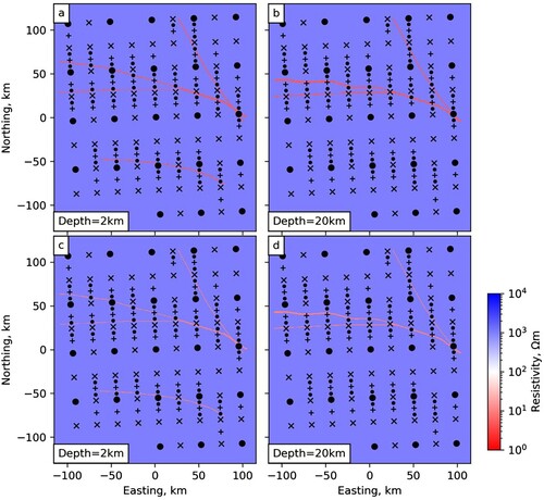
In all scenarios, the background rock resistivity was set to 1000 ohm-m which represents a typical value for upper crustal lithologies (e.g. Palacky 1988). Additional to Scenarios 1 and 2, a third scenario (Scenario 3) was considered in which the model setup was the same as Scenario 1 but at all sites on a half or full degree of latitude and longitude only periods >10 s were included in the inversion (compared the full broadband range of 0.001–1000 s at other sites). Thus Scenario 3 would represent a situation where a broadband survey was conducted omitting sites where long-period (e.g. AusLAMP) measurements had already been made.

MT inversion

We calculate the forward responses of our model using the ModEM 3D MT code (Egbert and Kelbert 2012; Kelbert et al. 2014) on a station grid that progressively densifies near the surface location of the faults as follows (Figure 2):

• ∼55 km (0.5°) spacing everywhere (base grid) +

• ∼28 km (0.25°) spacing within ∼55 km (0.5°) of fault location at surface +

• ∼14 km (0.125°) spacing (N-S direction only) within ∼28 km (0.25°) of fault location at surface +

• ∼7 km (0.0625°) spacing (N-S direction) within ∼14 km (0.125°) of fault location at surface

We calculate the forward responses onto a period range corresponding to broadband data (0.001–1000 s).

We add Gaussian noise as follows:

• The Z_XY and Z_XX components have Gaussian noise added as 5% of Z_XY.

• The Z_YX and Z_YY components have Gaussian noise added as 5% of Z_YX.

• The vertical components (tippers) have Gaussian noise added scaled by magnitude 0.02.

Standard errors for the inversions are then set to be consistent with the above Gaussian noise.

For each scenario, we run 3D inversions using ModEM with the four station densities above. For Scenario 1, an additional three inversions were run on a coarser vertical mesh, described below. All inversions were carried out on a coarser horizontal model mesh than that at which the forward model was computed, with cell sizes selected to be roughly 1/5 to 1/3 of station spacing (Table 1). Model covariance was set to 0.6 for all models, although models with a covariance of 0.3 were also run, showing little difference in the ability to resolve structures, and are provided in the Appendix (Figure A5–A7). The vertical mesh was 100 m at the surface increasing logarithmically to a target depth of 100 km followed by padding, a total of 120 vertical cells. In addition, a coarser vertical mesh was tested for the ∼14, ∼28 and ∼55 km station spacing in Scenario 1 as listed in the bottom three rows of Table 1. The coarser mesh was designed such that the aspect ratio of the cells at 40 km depth is approximately equal to 1. It also starts with 100 m thickness at the surface and extends to 100 km, but has fewer vertical cells and a corresponding larger increase factor in cell thickness.

Table 1. Mesh parameters used for inversion of synthetic data.

Station spacing (°)	Min station spacing N-S (km)	Min station spacing E-W (km)	Horizontal cell size (km)	Number of vertical cells	Vertical cell size at 40 km depth (km)	RMS misfit (Scenario 1)	RMS misfit (Scenario 2)	RMS misfit (Scenario 3)
0.5	55	47	10	120	1.4	2.14	1.74	2.47
0.25	28	24	6	120	1.4	1.85	1.60	1.75
0.125	14	24	3	120	1.4	1.71	1.49	1.91
0.0625	6.9	24	1.5	120	1.4	1.69	1.87	1.66
0.5	55	47	10	30	10.5	2.25
0.25	28	24	6	40	6.7	1.89
0.125	14	24	3	60	3.5	1.70

Recovered resistivity

All inversions reached an RMS misfit of between 1.49 and 2.47 (Table 1). The misfit generally improves with decreasing site spacing and model cell size. The inversions are shown at depths of 2 km (Figure 3), 20 km (Figure 4) and 10 km (Figure A1) and as a vertical slice at 0 km E from the surface down to 50 km depth (Figure 5). Additional vertical slices are shown in Figures A2 to A4. In Scenarios 1 and 2, with broadband deployments simulated at every site, the ∼28 km station spacing is a marked improvement compared to the ∼55 km station spacing in that it defines the fault network reasonably well as linear features, even at 2 km depth. However, the faults are segmented, and poorly defined in some areas (Figure 3 (b, f and j)). This is particularly the case in Scenario 2, in which the synthetic faults are narrower and less conductive, and the linear coherency, in particular of the north-northwest trending fault, is not clear (Figure 3 (f)). In contrast, both the ∼14 km and ∼7 km station spacing provide significant improvement in the definition of the faults, with the main difference being that the ∼7 km spacing resolves the fault to be narrower than the ∼14 km spacing, providing a higher localisation accuracy. In both scenarios the ∼55 km spacing images the shallow conductive structure poorly as might be expected (Figure 3 (a, e and i)), but the deeper structure is imaged in Scenarios 1 and 3 with the central fault corridor, which consists of two splay faults, appearing as a broad east–west striking conductive zone at 20 km depth (Figure 4 (a and i)).

Figure 3. Depth slices at 2 km showing inverted resistivity from progressively densified MT arrays with minimum station spacing of ∼55 km (0.5°), ∼28 km (0.25°), ∼14 km (0.125°), and ∼7 km (0.0625°). Top panel (a–d) shows Scenario 1 (750–1500 m wide fault, 5 Ωm, Figure 2 (a and b)); middle panel (e-h) shows Scenario 2 (500–1000 m wide fault, 10 Ωm, Figure 2 (c and d)), bottom panel (i–l) shows Scenario 3 (same as Scenario 1 but all sites on even 0.5 degree (∼55 km) intervals of latitude and longitude were inverted with only long-period data). Stations with short-period data (>0.001 s) are shown as dots, stations with only longer-period data (>10 s) are shown as crosses.

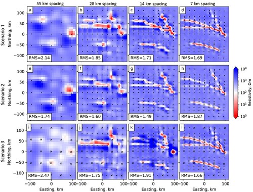
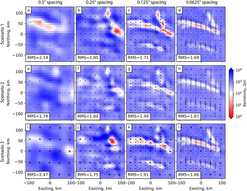
Figure 4. Depth slices at 20 km showing inverted resistivity from progressively densified MT arrays with minimum station spacing of ∼55 km (0.5°), ∼28 km (0.25°), ∼14 km (0.125°), and ∼7 km (0.0625°). Top panel (a–d) shows Scenario 1 (750–1500 m wide fault, 5 Ωm, Figure 2 (a and b)); middle panel (e–h) shows Scenario 2 (500–1000 m wide fault, 10 Ωm, Figure 2 (c and d)); bottom panel (i–l) shows Scenario 3 (same as Scenario 1 but all sites on even 0.5 degree (∼55 km) intervals of latitude and longitude were inverted with only long-period data). Stations with short-period data (>0.001 s) are shown as dots, stations with only longer-period data (>10 s) are shown as crosses.

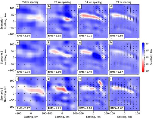
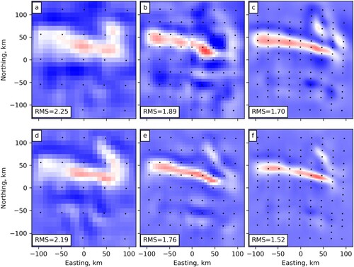
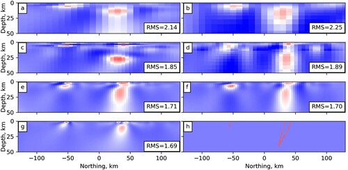
Figure 5. North-south section through the centre of the model for Scenario 1 (0 km E) showing the inversions from progressively densified data with spacing equal to ∼55 km (0.5°; top panel), ∼28 km (0.25°; second panel), ∼14 km (0.125°; third panel), and ∼ 7 km (0.0625°; bottom left panel). Bottom right panel (h) shows the true model. Left panel (a, c, e and g) shows the main inversions as presented in Figure 3, while b, d, f show models with a coarser vertical mesh (text and Table 1).

In Scenario 3, in which only periods >10 s were used at stations on exact 0.5 or 1° intervals (indicated by cross symbols in Figures 3–4), both the ∼28 km and ∼14 km station spacing provide noticeably poorer definition of the faults at 2 km depth (Figure 3 (j–k)) compared to Scenario 1 where the shorter-period data were included at these sites (Figure 3 (b–c)). The difference is much less significant for the ∼55 km and ∼7 km spacing. At a depth of 20 km, the difference between including and not including shorter periods is minimal for all survey designs.

In transect view (Figure 5 and Figures A2 to A4), the faults are imaged to be considerably wider compared to the true model, and are mostly not imaged to their full depth extent. In models with smaller station spacing, the width imaged broadly resembles the extent of the structure in birds-eye view, and the dip direction can be recognised (Figure 5 (e–g)). In the models with wider station spacing the structures appear wider, with the dip direction often ambiguous (Figure 5 (a–d)).

In almost all the station grid configurations, the faults are imaged as two oblate conductors that may or may not be connected, as opposed to one vertical, planar conductor. This is the case both in the inversions with fine and coarse vertical meshes, although the coarser vertical meshes generally resolve the conductors as more elongated vertically (Figure 5, Figures A2 (b, d, f) and A3 (b, d, f)).

Discussion

Synthetic modelling demonstrates that broadband MT measurements with a station spacing of ∼14 km across strike and ∼28 km along strike, are sufficient to resolve a laterally continuous 500 m to 1000 m-wide conductive fault zone, although tighter spacing provides increased coherency and more precise definition of its extent and geometry. This is an important result as it suggests that a relatively wide spacing of ∼28 km to ∼14 km, only $\frac{1}{2}$ to $\frac{1}{4}$ of the resolution of AusLAMP, may be sufficient to trace conductors from lower crustal depths into the upper crust, and represents a feasible next scale for examining features of interest in AusLAMP models.

At a station spacing of ∼28 km to ∼ 14 km, collecting high-frequency data (i.e. periods from 0.001–10 s) at sites where long-period data already exist, provides increased definition of the fault at shallow depths (e.g. 2 km) but marginal improvements for surveys with larger and smaller station spacing. This is likely because, at a station spacing of ∼55 km, neither broadband nor long-period only data are sufficient to resolve such a narrow structure effectively, whilst in the case of ∼7 km spacing, the station spacing is close enough that the missing short periods at the ∼55 km sites are compensated for adequately by adjacent sites. At mid- to upper crustal depths (20 km), the Scenario 3 survey designs with short-period data missing at the ∼55 km sites image the structure adequately. Therefore, the improvement when periods <10 s are added to these sites is marginal. Depths of ∼10 km (Figure A1) represent an intermediate level between the two depths shown in Figures 3 and 4. The four faults are imaged as semi-continuous features in the survey designs with station spacing down to ∼14 km and ∼7 km, and while omitting short periods at the ∼55 km sites reduces the continuity of these features, they are still recognisable. However, the survey design with spacing down to ∼28 km images the faults poorly at this depth.

The vertical extents of the faults in our inversions are generally not well resolved. The inability of MT to resolve the vertical extent of conductors is a well-known phenomenon and is consistent with previous synthetic modelling studies in which vertical, conductive features have been resolved shallower than their true depth (e.g. Martí et al. 2020; Unsworth and Bedrosian 2004). In our case, the faults also have a tendency to be split into two separate conductors, often at depths around the upper to middle crust transition. This is likely to be partly a function of inversion parameters and mesh construction. However, while vertical grid configuration makes some difference to how these features are recovered in an inversion (Figure 5 and Figures A2 to A4), a coarse vertical mesh does not completely resolve the issue. Moreover, in a real-world scenario, where the true structure will be unknown and will likely consist of features with a range of dips and laterally variable conductivity, it is impossible to design a mesh that will facilitate the recovery of the true structures. This result highlights the importance of thorough testing of the vertical mesh when carrying out sensitivity testing in MT inversion. It also highlights that it is important to understand the limitations of MT inversion when interpreting resistivity models derived from MT data, and warrants a note of caution when assessing the interconnectivity of fault/fluid pathway systems through the crust. As a consequence, it is of particular importance in an exploration scenario to consider that a lack of conductor interconnectivity, for example to a lower crustal/upper mantle source region, might be apparent only, and is not necessarily an indication of diminished prospectivity.

This contribution proposes an avenue into the optimisation of 3D MT survey design via synthetic modelling. Our model setup represents a first order approximation to real-world scenarios. It is worth noting that real-word structures are likely to display variability with depth and along strike with regards to factors such as interconnectivity and presence and type of conductive material (e.g. Bourlange et al. 2003; Moore et al. 1995; Morrow, Lockner, and Hickman 2015; Ritter et al. 2005). Using our approach, future work could systematically explore if and to what degree a more variable fault-conductivity network needs to be considered during survey design.

Conclusions

We present synthetic modelling to investigate the effectiveness of different MT survey designs in imaging a sub-vertical to moderately dipping crustal-scale fault network in a scenario that resembles a regional infill study as a follow up to a ∼55 km spaced long-period survey. We show that:

• Station spacing of ∼14 km (across strike) to ∼28 km (along strike) is adequate for tracing a planar fault zone with laterally coherent conductivity signature from the lower crust to the near surface.

• At these resolutions, broadband measurements at locations where long-period data already exist provide improvement in the resolved structure and are therefore worth doing.

• The coherency of vertical or near-vertical planar conductive features such as fault zones may not be imaged well in inversion, thereby highlighting the need for rigorous sensitivity testing of the vertical mesh.

• Synthetic modelling is a powerful tool not only to gain important insights for the interpretation of MT inversion data, but also for the optimisation of regional survey design.

Acknowledgements

This contribution forms part of Geoscience Australia’s Exploring for the Future program. The authors thank Gary Egbert and Anna Kelbert for providing access to the ModEM 3D inversion code used to run the forward models and inversions. The MTPy software (Kirkby et al. 2019; Krieger and Peacock 2014) was used to set up, run, and visualise both the forward models and the inversions presented in this paper. Resources from the National Computational Infrastructure were used to run the forward models and inversions. We thank Geoscience Australia reviewers Adrian Hitchman and Andy Clark, as well as two anonymous reviewers, for their constructive comments. This paper is published with the permission of the CEO, Geoscience Australia.

Disclosure statement

No potential conflict of interest was reported by the author(s).

Appendix

Additional depth slices

We present here model slices at 10 km depth for each of the scenarios discussed in the main paper.

Figure A1. Depth slices at 10 km showing inverted resistivity from progressively densified MT arrays with minimum station spacing of 0.5, 0.25, 0.125, and 0.0625 degrees of latitude/longitude (approximately 55, 28, 14 and 7 km). Top panel (a–d) shows Scenario 1 (750–1500 m wide fault, 5 Ωm, Figure 2 (a and b) of main manuscript); middle panel (e–h) shows Scenario 2 (500–1000 m wide fault, 10 Ωm, Figure 2 (c and d) of main manuscript); bottom panel (i–l) shows Scenario 3 (same as Scenario 1 but all sites on even 0.5 degree (∼55 km) intervals of latitude and longitude were inverted with only long-period data). Stations with short-period data (>0.001 s) are shown as dots, stations with only long-period data (>10 s) are shown as crosses.

Additional vertical slices

We present here additional vertical slices to those presented in the main text. Figures A2 and A3 show the comparison between Scenario 1 and Scenario 1 with a coarser vertical mesh, at different eastings (−50 and +50 km E). Figure A4 shows vertical sections (at 0 km E) for Scenarios 2 and 3.

Figure A2. North–south section at −50 km E showing inversions from Scenario 1 and Scenario 1 with a coarser vertical mesh using progressively densified data arrays with spacing across strike equal to ∼55 km (0.5°; top panel), ∼28 km (0.25°; second panel), ∼14 km (0.125°; third panel), and ∼ 7 km (0.0625°; bottom left panel). Bottom right panel (h) shows the true model. Left panel (a, c, e and g) shows the main inversions as presented in Figure 3 of the main manuscript, b, d, f shows models with a coarser vertical mesh (main manuscript text and Table 1).

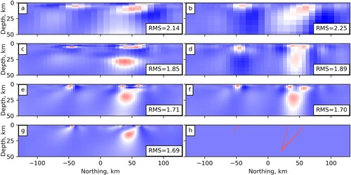
Figure A3. North-south section at 0 km E showing inversions from Scenario 1 and Scenario 1 with a coarser vertical mesh using progressively densified data arrays with spacing across strike equal to ∼55 km (0.5°; top panel), ∼28 km (0.25°; second panel), ∼14 km (0.125°; third panel), and ∼ 7 km (0.0625°; bottom left panel) . Bottom right panel (h) shows the true model. Left panel (a, c, e and g) shows the main inversions as presented in Figure 3 of the main manuscript, b, d, f shows models with a coarser vertical mesh (main manuscript text and Table 1).

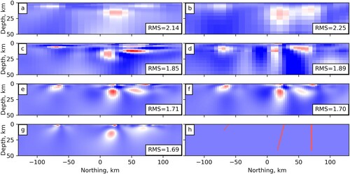
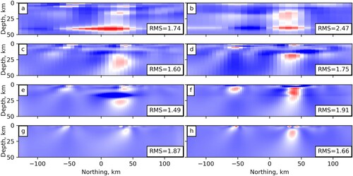
Figure A4. North-south section at 0 km E showing inversions from Scenarios 2 and 3 using progressively densified data arrays with spacing across strike equal to ∼55 km (0.5°; top panel), ∼28 km (0.25°; second panel), ∼14 km (0.125°; third panel), and ∼ 7 km (0.0625°; bottom panel). Left panel (a, c, e and g) shows Scenario 2 discussed in the main text with the narrower, less conductive fault zone setup; b, d, f and h show Scenario 3 (see main manuscript text and Table 1 for further details).

Runs with different covariance

We present here some model runs carried out with a lower covariance of 0.3. These show that the ability to resolve the fault structure is not affected by reducing the covariance.

Figure A5. Depth slices at 2 km showing inverted resistivity from the synthetic data of Scenario 1 (coarse vertical mesh) in the main text, with a covariance of 0.6 as used in the main text (top panel) and 0.3 (bottom panel). Minimum station spacing of (a and d) ∼55 km (0.5°); (b and e) ∼28 km (0.25°); and (c and f) ∼14 km (0.125°).

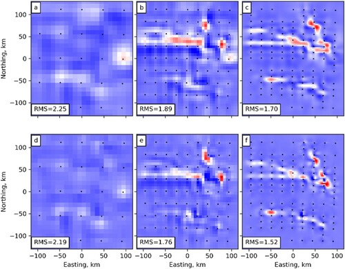
Figure A6. Depth slices at 10 km showing inverted resistivity from Scenario 1 (coarse vertical mesh) in the main text, with a covariance of 0.6 as used in the main text (top panel) and 0.3 (bottom panel). Minimum station spacing of (a and d) ∼55 km (0.5°); (b and e) ∼28 km (0.25°); and (c and f) ∼14 km (0.125°).

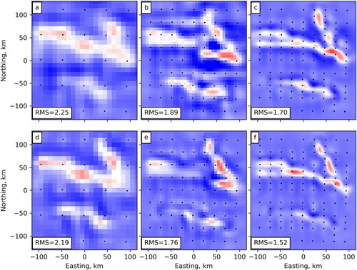
Figure A7. Depth slices at 20 km showing inverted resistivity from Scenario 1 (coarse vertical mesh) in the main text, with a covariance of 0.6 as used in the main text (top panel) and 0.3 (bottom panel). Minimum station spacing of (a and d) ∼55 km (0.5°); (b and e) ∼28 km (0.25°); and (c and f) ∼14 km (0.125°).

References

- Bourlange, S., P. Henry, J.C. Moore, H. Mikada, and A. Klaus. 2003. Fracture porosity in the décollement zone of Nankai accretionary wedge using logging while drilling resistivity data. Earth and Planetary Science Letters 209 no. 1: 103–112. doi:10.1016/S0012-821X(03)00082-7.
- Calvert, A.J., and M.P. Doublier. 2018. Archaean continental spreading inferred from seismic images of the Yilgarn Craton. Nature Geoscience 11 no. 7: 526–530. doi:10.1038/s41561-018-0138-0.
- Celestino, M.A.L., T.S.d. Miranda, G. Mariano, M.d.L. Alencar, B.R.B.M.d. Carvalho, T.d.C. Falcão, J.G. Topan, J.A. Barbosa, and I.F. Gomes. 2020. Fault damage zones width: implications for the tectonic evolution of the northern border of the Araripe Basin, Brazil, NE Brazil. Journal of Structural Geology 138: 104116. doi:10.1016/j.jsg.2020.104116.
- Chiang, C.W., M.J. Unsworth, C.S. Chen, C.C. Chen, A.T. Lin, and H.L. Hsu. 2008. Fault zone resistivity structure and monitoring at the Taiwan Chelungpu drilling project (TCDP). Terrestrial, Atmospheric and Oceanic Sciences Journal 19: 473–479. doi:10.3319/TAO.2008.19.5.473(T).
- Choi, J.-H., P. Edwards, K. Ko, and Y.-S. Kim. 2016. Definition and classification of fault damage zones: A review and a new methodological approach. Earth-Science Reviews 152: 70–87. doi:10.1016/j.earscirev.2015.11.006.
- Duan, J., W. Jiang, D. Kyi, and M. Costelloe. 2020. AusLAMP: Imaging the Australian lithosphere for resource potential, an example from northern Australia. Extended abstract, Exploring for the Future, 1-4.
- Duan, J., and D. Kyi. 2018. Australian Lithospheric Architecture Magnetotelluric Project (AusLAMP): Victoria: Data Release Report. Geoscience Australia. doi:10.11636/Record.2018.021.
- Duan, J., D. Kyi, and W. Jiang. 2021. Application of Multi-Scale Magnetotelluric Data to Mineral Exploration: An Example from the East Tennant Region, Northern Australia. Geophysical Journal International 229 no. 3: 1628–1645. doi:10.1093/gji/ggac029.
- Duan, J., D. Taylor, K. Czarnota, R. Cayley, and R. Chopping. 2016. AusLAMP MT over Victoria: New insight from 3D modelling highlights regions of anomalously conductive mantle and unexpected linear trends in the crust. http://www.publish.csiro.au/ex/pdf/ASEG2016ab284.
- Egbert, G.D., and A. Kelbert. 2012. Computational recipes for electromagnetic inverse problems. Geophysical Journal International. doi:10.1111/j.1365-246X.2011.05347.x.
- Heinson, G., Y. Didana, P. Soeffky, S. Thiel, and T. Wise. 2018. The crustal geophysical signature of a world-class magmatic mineral system. Scientific Reports 8 no. 1: 1–6. doi:10.1038/s41598-018-29016-2.
- Jiang, W., J. Duan, M. Doublier, A. Clark, A. Schofield, R. Brodie, and J. Goodwin. 2022. Mapping Crustal Structures through Scale Reduction Magnetotelluric Survey in the East Tennant Region, Northern Australia. Geoscience Australia Extended Abstracts, Exploring for the Future.
- Kelbert, A., N. Meqbel, G.D. Egbert, and K. Tandon. 2014. ModEM: A modular system for inversion of electromagnetic geophysical data. Computers and Geosciences. doi:10.1016/j.cageo.2014.01.010.
- Kirkby, A., R.J. Musgrave, K. Czarnota, M.P. Doublier, J. Duan, R. Cayley, and D. Kyi. 2020. Lithospheric architecture of a Phanerozoic orogen from magnetotellurics: AusLAMP in the Tasmanides, southeast Australia. Tectonophysics 793. doi:10.1016/j.tecto.2020.228560.
- Kirkby, A., F. Zhang, J. Peacock, R. Hassan, and J. Duan. 2019. The MTPy software package for magnetotelluric data analysis and visualisation. Journal of Open Source Software 4 no. 37: 1358–1358. doi:10.21105/joss.01358.
- Korsch, R.J., and M.P. Doublier. 2016. Major crustal boundaries of Australia, and their significance in mineral systems targeting. Ore Geology Reviews 76: 211–228. doi:10.1016/J.OREGEOREV.2015.05.010.
- Krieger, L., and J.R. Peacock. 2014. MTpy: A python toolbox for magnetotellurics. Computers & Geosciences 72: 167–175. doi:10.1016/J.CAGEO.2014.07.013.
- Kyi, D., J. Duan, A. Kirkby, and N. Stolz. 2020. Australian Lithospheric Architecture Magnetotelluric Project (AusLAMP): New South Wales: data release (Phase one). Geoscience Australia. doi:10.11636/Record.2020.011.
- Martí, A., P. Queralt, A. Marcuello, J. Ledo, E. Rodríguez-Escudero, J.J. Martínez-Díaz, J. Campanyà, and N. Meqbel. 2020. Magnetotelluric characterization of the Alhama de Murcia Fault (Eastern Betics, Spain) and study of magnetotelluric interstation impedance inversion. Earth, Planets and Space 72 no. 1: 16. doi:10.1186/s40623-020-1143-2.
- Moore, J.C., T.H. Shipley, D. Goldberg, Y. Ogawa, F. Filice, A. Fisher, M.J. Jurado, et al. 1995. Abnormal fluid pressures and fault-zone dilation in the Barbados accretionary prism: evidence from logging while drilling. Geology 23 no. 7: 605–608. doi:10.1130/0091-7613(1995)023<0605:AFPAFZ>2.3.CO;2.
- Morrow, C., D.A. Lockner, and S. Hickman. 2015. Low resistivity and permeability in actively deforming shear zones on the San Andreas Fault at SAFOD. Journal of Geophysical Research: Solid Earth 120 no. 12: 8240–8258. doi:10.1002/2015JB012214.
- Palacky, G.J. 1988. 3. Resistivity characteristics of geologic targets. In Electromagnetic methods in applied geophysics: Volume 1, Theory, ed. Misac N. Nabighian, 52–129. Society of Exploration Geophysicists. doi:10.1190/1.9781560802631.ch3
- Pearce, C.I., R.A.D. Pattrick, and D.J. Vaughan. 2006. Electrical and magnetic properties of sulfides. Reviews in Mineralogy and Geochemistry 61 no. 1: 127–180. doi:10.2138/rmg.2006.61.3.
- Ritter, O., A. Hoffmann-Rothe, P.A. Bedrosian, U. Weckmann, and V. Haak. 2005. Electrical conductivity images of active and fossil fault zones. In High-strain zones: structure and physical properties (Vol. 245), eds. D. Bruhn, and L. Burlini, 165–186 Geological Society of London. doi:10.1144/GSL.SP.2005.245.01.08.
- Robertson, K., G. Heinson, and S. Thiel. 2016. Lithospheric reworking at the Proterozoic–Phanerozoic transition of Australia imaged using AusLAMP Magnetotelluric data. Earth and Planetary Science Letters. doi:10.1016/j.epsl.2016.07.036.
- Robertson, K., S. Thiel, and G. Heinson. 2018. Evolving 3D lithospheric resistivity models across southern Australia derived from AusLAMP MT. ASEG Extended Abstracts 2018 no. 1: 1–5. doi:10.1071/ASEG2018abM2_1G.
- Thiel, S., B.R. Goleby, M.J. Pawley, and G. Heinson. 2020. AusLAMP 3D MT imaging of an intracontinental deformation zone, Musgrave Province, Central Australia. Earth, Planets and Space 72 no. 1: 98. doi:10.1186/s40623-020-01223-0.
- Thiel, S., A. Reid, G. Heinson, and K. Robertson. 2016. Insights into lithospheric architecture, fertilisation and fluid pathways from AusLAMP MT. ASEG Extended Abstracts 2016 no. 1: 1–6. doi:10.1071/ASEG2016ab261.
- Unsworth, M., and P.A. Bedrosian. 2004. Electrical resistivity structure at the SAFOD site from magnetotelluric exploration. Geophysical Research Letters 31 no. 12. doi:10.1029/2003GL019405.
- Vella, L., and D. Emerson. 2012. Electrical Properties of Magnetite- and Hematite-Rich Rocks and Ores. ASEG Extended Abstracts 2012: 26–29.
- Wang, L., J. Duan, and J. Simpson. 2018. Electrical conductivity structures from magnetotelluric data in Cloncurry Region. Record. doi:10.11636/Record.2018.005.