Predictive Analytics Machinery for STEM Student Success Studies

ABSTRACT

Statistical predictive models play an important role in learning analytics. In this work, we seek to harness the power of predictive modeling methodology for the development of an analytics framework in STEM student success efficacy studies. We develop novel predictive analytics tools to provide stakeholders automated and timely information to assess student performance toward a student success outcome, and to inform pedagogical decisions or intervention strategies. In particular, we take advantage of the random forest machine learning algorithm, proposing a number of innovations to identify key input thresholds, quantify the impact of inputs on student success, evaluate student success at benchmarks in a program of study, and obtain a student success score. The proposed machinery can also tailor information for advisers to identify the risk levels of individual students in efforts to enhance STEM persistence and STEM graduation success. We additionally present our predictive analytics pipeline, motivated by and illustrated in a particular STEM student success study at San Diego State University. We highlight the process of designing, implementing, validating, and deploying analytical tools or dashboards, and emphasize the advantage of leveraging the utilities of both statistical analyses and business intelligence tools in order to maximize functionality and computational capacity.

Introduction

Background: literature review of STEM student success studies

Increasing the number of graduates who are prepared for STEM occupations has become a national priority for maintaining U.S. competitiveness in a global economy (Carnevale, Smith, and Melton 2011). According to the 2012 report by the President’s Council of Advisors on Science and Technology (PCAST), the United States will need an additional one million STEM professionals over the next decade on top of current projections. Thus, it is important for universities to improve student retention and graduation success in STEM majors in order to meet the projected demand.

Many recent studies point to the importance of mathematical skill preparation for students before entering a STEM major (Benbow 2012; Brown, Halpin, and Halpin 2015; Kassaee and Rowell 2016; Sadler and Tai 2007; Tai, Sadler, and Mintzes 2006; Wilson and Shrock 2001). However, the performance of U.S. students on science and mathematics tests is consistently below the international average (PCAST, 2012; OECD, 2012). For instance, mathematics performance rankings for 15-year-old U.S. students declined to 27th in 2012, according to the results from the Program for International Student Assessment (PISA). Moreover, statistics show that, in general, female and underrepresented minority (URM) students have high attrition rates compared to other groups (Besterfield-Sacre, Atman, and Shuman 1997; Fleming et al. 2008; Mitchell and Daniel 2007). These groups of students are less likely to enroll in STEM majors at entrance to university, and those that enter as a STEM major are more likely to switch out of STEM or fail to graduate (Alkasawneh and Hobson, 2009; Chen and Soldner 2013; Peterson et al. 2011; Urban, Reyes, and Anderson-Rowland 2002). Features, such as ethnicity and URM are important factors toward identifying at-risk students, and developing strategies to optimally allocate resources to these subgroups. In addition, a STEM student’s decision to persist in or change out of STEM occurs primarily in their first year or two of college (Chen and Soldner 2013; Kassaee and Rowell 2016; PCAST 2012). This decision is based on successful completion of a gateway course, which is usually a quantitatively oriented class, such as calculus (Brown, Halpin, and Halpin 2015). The PCAST (2012) report also notes that high-performing students often switch majors due to uninspiring introductory courses. On the flip-side, low-performing students with a strong interest in and passion for STEM struggle with certain introductory courses due to insufficient mathematics preparation and support networks (PCAST 2012). These introductory courses thus become a major road block to student achievement in STEM (Thiel, Peterman, and Brown 2008). Therefore, a focus on identifying and managing courses that frequently hinder graduation may be a strategic solution to aid STEM students achieve their academic goal.

Previous studies emphasize the importance of identifying college students with higher risk of dropping out in early stages (Herzog 2006; Lin, Imbrie, and Reid 2009), and indicate that early intervention/advising is effective in improving STEM students’ retention and graduation rates (Zhang et al. 2014). Early Warning Systems (EWS) use predictive algorithms to provide data-driven early warning indicators (EWI) to identify at-risk students within courses or degree programs (Beck and Davidson 2001; Griff and Matter 2008; Lee et al. 2015; Macfadyen and Dawson 2010; Neild, Balfanz, and Herzog 2007). Present studies on EWS are conducted mostly on student academic information collected prior to college (e.g., demographic data, high school GPA, SAT scores; Dobson 2008; Eddy, Brownell, and Wenderoth 2014; Lee et al. 2008; Orr and Foster 2013; Rath et al. 2007; Richardson, Abraham, and Bond 2012), and much less frequently on academic performance data gathered during a student’s tenure at university (e.g., course grades, term GPA, term units). Lee et al. (2015) conduct a study on EWS using data from student university academic performance. However, the paper focuses only on student performance in large STEM courses. Therefore, we are motivated to develop and construct an analytics system that automatically processes data from a complex student information database, where both student pre-university and university academic data is recorded.

Traditional methods of statistical analysis have been used to predict student graduation/retention in STEM studies, including logistic regression (Dika and D’Amico 2016; Thompson, Bowling, and Markle 2018; Whalen and Shelley 2010), discriminant analysis (Burtner 2005; Raelin et al. 2015; Redmond-Sanogo, Angle, and Davis 2016), structural equation models (Simon et al. 2015), and survival analysis (Ameri et al. 2016; Murtaugh, Burns, and Schuster 1999). The advantage of these traditional methods is that they can easily quantify the contribution of each factor on student success. However, for complex or unstructured data (e.g., data derived from a student information database, holding thousands of records over numerous academic terms), the assumptions underlying these models (in particular distributional assumptions for significance tests and multicollinearity) are quickly violated.

Data mining techniques are becoming more popular and accurate to model student performance in higher education, and study student success in STEM fields. Alkhasawneh and Hobson (2011) develop two neural network models using a feed-forward back-propagation network to predict retention for students in science and engineering fields. Herzog (2006) adopts three-rule induction decision trees (C&RT, CHAID-based, and C5.0) and three back-propagation neural networks (simple-topology, multi-topology, and three hidden-layer pruned) with a multinomial logistic regression model to predict student retention and time to degree. The study indicates that the neural networks and decision tree algorithms outperform the multinomial logistic regression model with better accuracy when a large data set was used. Mendez et al. (2008) uses random forest to explore new variables that impact student persistence to a science or engineering degree, and compares the results between classification trees, random forest and logistic regression. The paper emphasizes the advantage and superiority of utilizing trees-based methods (classification trees and random forest) to identify complex relationships and important factors, and noted that these methodologies show promise for studying persistence to graduation in STEM fields.

Goals: predictive analytics and an analytics pipeline

The goals of this paper are two-fold. First, we introduce novel predictive analytics tools for an application in STEM student success studies. The methods development is driven by a series of questions we have found critical for decision-making by key administrative stakeholders in response to such studies. Within this goal, we also aim to provide a machine learning framework that may be automated and produces statistically informative visualizations for relatively easy absorption by users. Given the scale and depth of this first goal, we devote Predictive Analytics Algorithms section to this methods development.

Second, we discuss our analytics pipeline moving through the data curation and preparation phase as input to our machine learning methods, application of the analytics machinery, and then dashboard reporting performed to output results to campus stakeholders. Again, our aim is to provide a framework that may be automated, both for application in multiple student success studies and for updating as new student data is obtained each semester. Dashboards and An Analytics Pipeline section presents our pipeline, discussing dashboard development and implementation. Our focus is on STEM student success efficacy studies. For clarity and ease of exposition, we present our methods within the context of a study of graduation success of entering STEM majors at San Diego State University. The data and particular issue relating to student success are described in Study Data and Motivating Problem section.

In STEM student success efficacy studies, we are typically interested in answering a series of analytics queries concerning a student success outcome: (1) identify key factors affecting student success, (2) detect break points in key inputs (e.g., a grade in a given course or participation in interventions) that impact student success, (3) highlight successful paths as a student progresses toward the outcome of interest, quantify the impact of specific inputs (e.g., demographics or academic preparation/performance) on student success, and (4) gauge success of individual students, and identify their risk levels using a quantitative measure.

In this paper, we consider random forest as the machine learning tool for developing a methodological framework to address each of these analytics objectives. It has been shown that random forest consistently outperforms competing learning algorithms, such as neural networks, boosted trees and support vector machines (Caruana, Karampatziakis, and Yessenalina 2008; Caruana and Niculescu-Mizil 2006; Fernandez-Delgado et al. 2014). Details of analytics tools that have been used specifically in STEM student success studies will be further discussed in Predictive Analytics Algorithms section. Furthermore, random forest is a flexible tool, especially compared to regression modeling, for automating analytics tasks (James et al., Chapter 8). We also propose use of the R statistical software environment (R Core Team 2017) for our analytics tasks, and report study findings through a series of STEM student success dashboards.

Study data and motivating problem

Data for this paper were provided from the student information database in SDSU Analytic Studies & Institutional Research (ASIR). The population of interest was SDSU students enrolled in STEM majors as first-time freshmen from 2001 to 2016. In typical predictive model settings, there is at least one target (dependent) variable and multiple input (predictor/independent) variables. In the STEM study, the input variables span several aspects including demographic, educational background, at-risk indicators, and academic preparation and performance. The target variable is the graduation outcome, namely whether or not a student graduates in a pre-determined number of years. We consider 4, 5, and 6 year graduation rates. Table 1 lists the input and target variables. STEM majors are defined according to the STEM-Designated Degree Program List (SDDPL) released by the U.S. Immigration and Customs Enforcement (ICE) as of January, 2015. Note that the proposed methods may not be limited to STEM retention/success studies, and are generally applicable to a variety of efficacy studies in learning and academic analytics, at course, departmental, institutional, regional, national, and international level (Siemens and Long 2011).

Table 1. List of institutional variables considered in the STEM success study.

Demographic information

Gender

Age

Ethnicity

Disability status

Honors program

Low income status

Pell grant

Military status

EOP status

On-campus housing in dorms

Learning community – specialized dorms

Compact for Success – local outreach program

Academic preparation

SAT/ACT score

Math proficiency

English proficiency

High school GPA

ELM score

First generation college student

Major status

Admission basis – first-time freshman, transfer

Enrollment status – full-time or part-time

Academic Performance

Term/Total/Campus GPA

Term/Total/Campus units earned

Probationary status – each semester

Disqualified status – each semester

STEM major indicator – each semester

Grades in each course enrolled – initial time or last time taking

Semester each course enrolled

AP credit by subject

Courses transferred into SDSU for credit

Grades in transferred courses

Semester course transferred

Graduation outcomes

4-year graduation success indicator

5-year graduation success indicator

6-year graduation success indicator

Time to graduation – number of semesters or total units earned

Explore student retention problem: student movement into and out of STEM fields via the migration flow plot

Producing a sufficient amount of graduates for STEM occupations has risen as a national priority in the United States the past few years (Chen and Soldner 2013). According to the national data, more than 50% of freshmen entering college as a STEM major either switched to a non-STEM major or dropped out from college entirely without a degree (Chen and Weko 2009). At SDSU, of freshmen who enrolled in STEM at the start of their college career between 2001 and 2008, 30% graduated in STEM, 30% switched and graduated from a non-STEM major, and 40% failed to graduate within 6 years. Some recent U.S. policies have focused on increasing STEM retention, and suggest that even a small growth can contribute substantially to fulfilling the industry demand of STEM graduates (Ehrenberg 2010; Haag and Collofello 2008; PCAST 2012). Therefore, it is of critical importance for academic advisers to track students’ path into or out of STEM majors through automated data extraction and informative data visualization tools.

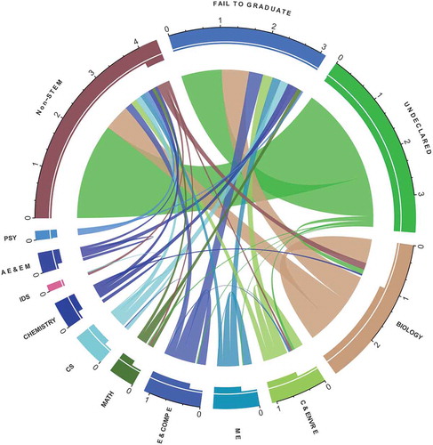
Figure 1 presents flow from the 10 top (by enrollment numbers) STEM departments, and one category representing students who did not declare a major on entrance to SDSU. The plot also shows flow to graduating in a non-STEM major and students that failed to graduate. Each pie wedge in the circle has, on the “crust”, an outer, thick-lined arc and an inner, thinner-lined arc. The outer, thick-lined arc presents the total number of students who either started or graduated in a given department. The inner, thinner-lined arc presents the number of students who enrolled in a given department upon entry. The color scheme identifies migration/flow of students from the major at entrance to the major at graduation. Since students can not graduate as undeclared, the undeclared wedge has only students entering and not exiting (outer and inner arcs are of identical length). On the other hand, fail to graduate is an exit outcome, so that wedge has no students entering (there is no inner arc). For example, the beige wedge shows that out of about 2,000 students entering as Biology majors during the period of study (inner arc), three beige flow lines appear: approximately 600 graduated in Biology (flow line within the department), 400 graduated in non-STEM majors (flow out), and 700 failed to graduate from any major (flow out). Moreover, three different colored flow lines appear: about 100 undeclared (green) and 100 non-STEM majors (dark brown), as well as a small group of Chemistry (dark blue) students switched into and graduated in Biology (flow in).

Figure 1. Circular migration plot for STEM students – Cohorts 2001 to 2008. Unit is 1000 per axis tick.

Department abbreviations are as follows: Psychology PSY, Aerospace Engineering and Engineering Mechanics AE & EM, Information and Decision Systems IDS; Chemistry and Biochemistry CHEMISTRY, Computer Science CS, Mathematics and Statistics MATH, Electrical and Computer Engineering E & COMP E, Mechanical Engineering ME, Civil, Construction and Environmental Engineering C & ENVR E. The circle “crust” includes an outer, thick-lined arc that represents the total volume of students moving to and/or from these departments/majors. The crust also includes an inner, thinner-lined arc that represents the number of students entering the university in these departments/majors.

The migration plot is also incorporated as a dashboard tool to provide a historical perspective and visualization of student movement between and out of STEM majors, and the proportion of STEM students that fail to graduate. Advisers and administrators can use this information to identify student migration patterns and address retention hurdles. The plot is a pre-cursor to deeper dives into potential root causes of STEM migration through the student advising dashboard presented later in the paper (Figure 9).

Figure 2. Important course predictor to graduation success with cutoff grade: the threshold is determined from the variable importance [Algorithm 1].

Figure 3. Sequential analysis plot: quantification of student migration within STEM and out of STEM based on performance in a key major pre-requisite progression course (here Calculus for Biology II). Note that the course grades are from the students’ first attempt at the course.

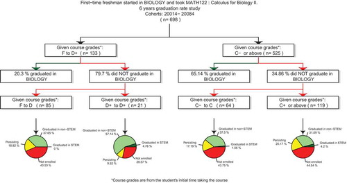
Figure 4. Success score gauge plot. Red zone represents “at risk” (), orange zone represents “warning” (10–25%), yellow zone represents “safe” (25–75%), light green zone represents “on track” (75–90%), and green zone represents “succeeding” (). The black arrow pointer indicates the success score for the student under consideration. The grey arrow pointer presents a predicted student success score following a behavioral change, for example an intervention strategy in which the student partakes or a change in performance.

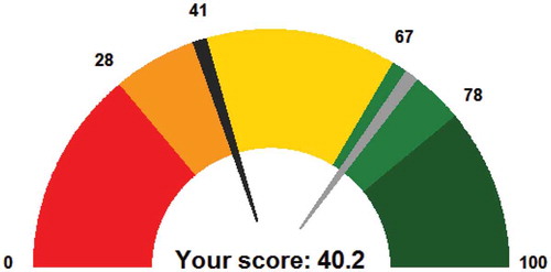
Figure 5. ROC curve using proposed analytic algorithms through random forest. Data was extracted for predicting the success of 1st, 2nd, 3rd, and 4th semester Biology students graduating in the same department within 6 years.

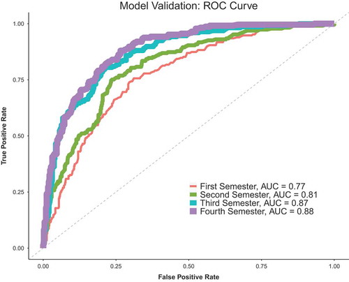
Figure 6. Conceptual representation of our analytics workflow for designing and deploying dashboards using the proposed predictive modeling outcomes.

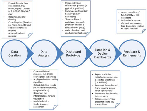
Figure 7. Conceptual representation of our workflow for prototyping and establishing the STEM student success dashboards. Though we use Tableau as our BI solution, any BI platform may be used in those workflow bubbles.

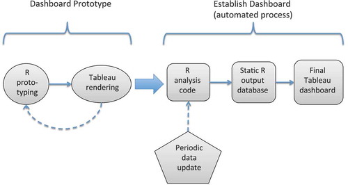
Figure 8. Screen shot of the prototype student success dashboard from R shiny dashboard.

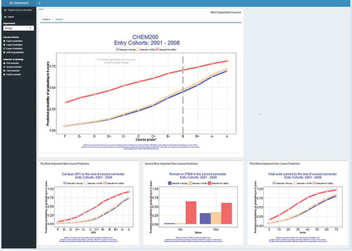
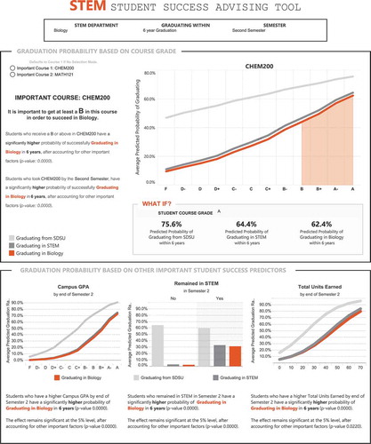
Figure 9. Screen shot of the student success dashboard from Tableau.

Predictive analytics algorithms

We propose random forest as the primary predictive modeling algorithm in our framework. Random forest (Breiman 2001) is an ensemble tree learning algorithm for classification or regression. In typical data mining applications, a data set is randomly split into a training data set for model construction and a testing data set for model assessment. In a random forest, each of a number of decision trees are grown based on a random sample selected with replacement (bootstrap sample) from the training data set. The decision rule at each (internal) node in a tree is chosen as having the optimal split over a subset of randomly selected predictors. After a random forest has been constructed, predictions for the testing set or for students with unobserved outcome are obtained by sending the new data through the forest. By averaging the predictions from all the individual trees in the forest, we obtain predictions for the testing set or for students with unobserved outcome. There are several advantages to random forest (James et al. 2013): (1) high predictive accuracy relative to competing machine learning algorithms (Caruana, Karampatziakis, and Yessenalina 2008; Caruana and Niculescu-Mizil 2006; Fernandez-Delgado et al. 2014); (2) smaller issue with over-fitting, compared to classification and regression trees (CART) and boosting (James et al. 2013, Chapter 8); (3) ease in handling correlations among and higher-order interactions between predictors; (4) unique insights into the data, variable importance, proximity matrix, and tree structure. That said, random forests are computationally costly, though efficiency may be gained through parallel/cluster computing. Furthermore, a single tree from CART (Breiman et al. 1984), and the corresponding branch decision rules, are easier to interpret than decision rules from a forest of decision trees. This latter challenge is particularly prominent if the goal is to identify a defined split rule (cut-off value) for a given predictor. Finally, missing data demands greater attention in a random forest. Missing data considerations are beyond the scope of this paper, though we will discuss options in Discussion section.

In this section, we will step through random forest methods and data mining visualizations we have developed or that we have reformulated from machine learning applications in other disciplines to address our predictive analytics needs. In addition to the migration plot (see Figure 1), these tools include (1) random forest variable importance ranking; (2) course grade indicator inputs; (3) marginal effects; (4) a student success score. We focus our development on the study of STEM program success to exposit the methods and visualizations around a well-defined illustration/application.

Identifying important predictors of STEM program success

The random forest method is known for providing variable importance ranking on all inputs (see e.g. James et al. 2013, Chapter 8). We will briefly outline the procedure in the first subsection and then introduce our random forest innovation for establishing important grade thresholds for key courses identified.

Random forest variable importance rankings

Breiman (2001, 2002) propose an algorithm to evaluate the importance of a particular predictor by summing the decrease in node impurity across all nodes where the predictor is used, and then averaging over all trees in the forest. Node impurity quantifies how well a tree splits the data. If a variable is important, a tree tends to split mixed labeled nodes into pure single class nodes. This option of measuring variable importance is known as the mean decrease Gini (MDI) or Gini importance index. Mean decrease accuracy (MDA) is an alternative measure for evaluating importance scores. The values of the predictor of interest are randomly permuted in an out-of-bag (OOB) sample. The idea is that if the variable is not important, then rearranging the values of that variable will not degenerate the prediction accuracy in the OOB sample. Several studies (Genuer et al. 2010; Strobl et al. 2008, 2007) have focused on studying the biases in MDI and MDA toward certain predictors, experimental evidence suggesting MDA for evaluating variable importance. In this study, we thus adopt MDA as the importance scores for predictors. In practice, the variable importance algorithm is embedded within the random forest procedure, and can be easily executed through numerous machine-learning related software.

Although random forest is sufficiently advanced to handle highly correlated predictors, it is a challenge to select and present important predictors, especially when highly correlated predictors are inclined to have similar importance scores. Therefore, we first ranked the entire set of predictors through the variable importance algorithm. For predictors that have similar characteristics, (e.g., term GPA, total GPA, and campus GPA), we chose and retained only the highest ranked one of the set based on the importance score. The predictors were categorized into course-level and non-course-related types. Only the highest ranked predictors from each type were selected for presentation, with statistical evaluation exported for dashboard development. Note that to ensure predictors with similar characteristics are highly correlated at first, correlation analysis and variance inflation factor (VIF) measures were employed for further justification.

Course grade indicators as random forest inputs

Cutoff scores in exam, GPA, etc. have been widely used as part of decision-making at higher education institutions. Although there may not always be natural breakpoints in the scores, in many circumstances, the institutions need to establish certain rules to categorize students for multiple purposes. For instance, SAT/ACT cutoff score and high school GPA cutoff have been used as admission criteria. Moreover, placement exam cutoffs are set to determine what level of a given subject (e.g., mathematics) a student should take upon entrance to the university. Prerequisite course performance thresholds are utilized as a selection criterion for enrolling students in pre-professional programs (e.g., nursing, pre-med, business). Inspired by these examples, we are motivated to identify grade thresholds in potentially multiple courses for STEM student success, with respect to persisting and graduating in a STEM major.

Random forests can lend naturally to the identification of a cut-point. In particular, we may for each student construct a series of grade-point indicators; namely did the student score an A− or better, did the student score a B+ or better, did the student score a B or better, etc. The random forest variable importance ranking routine will then identify the indicator (grade-point cut-off) most predictive of STEM program success. Algorithm 1 presents the pseudocode for our method. Note that the course grade predictors are replaced by newly created course grade-point indicators while leaving all other variables intact. In order to identify the most important courses and their grade threshold, the following approach was used: first, we select the top 10 predictors of student graduation success based on variable importance ranking, and then divide them into course and non-course categories. The courses and grade cut-point appearing in the course category are identified as important courses with the corresponding key grade threshold. In cases where there may be more than one course grade-point indicator for the same course, we single out the highest ranked one.

Though the grade-point ranges overlap across the indicators, the collinearity creates no difficulties for the random forest in this context. Furthermore, these indicators lend to quantification of the probability of success at each course grade level; we will develop this method in Marginal Effects section. Figure 2 illustrates the most important grade cut-point (a grade of B) in MATH 122: Calculus for Biology II for success in the Biology major program (grey vertical dashed line). The trend lines present the marginal effects to be discussed in Marginal Effects section (blue line for graduating in the same department as entry; yellow line for graduating in STEM; red line for graduating in any major).

Algorithm 1 Random forest with course-grade indicator

1: Given a time point , extract course grades received at , where .

2: For each course , create indicator (Yes or No); at each grade level .

3: Replace course grades with indicators as new predictors, leaving all other variables intact.

4: Use the data (outcome and all predictors) to construct the random forest.

5: Obtain the predicted probability of success by averaging across all observations.

6: Obtain variable importance, and rank the predictors from the most to the least important.

7: Obtain the highest ranked indicator for course .

Successfully progressing through a program: sequential analysis and visualization

The identified key courses and course grade cut-points predictive of graduation success from Identifying Important Predictors of STEM Program Success section may be used to further study migration between STEM programs and out of STEM. We initiate our analysis by extracting the students who start in a particular STEM major, and investigate success graduating in the same major (Level 1). Algorithm 1 is applied to identify the course-grade threshold (). We then extract the students who failed to graduate in the same major, and investigate success graduating in other STEM majors (Level 2). At this level, new course-grade thresholds () are identified, conditioning on . We lastly present a graphic of current academic status statistics for students who failed to graduate in STEM (Level 3). Figure 3 presents the resulting infographic.

Marginal effects

The course grade indicators as discussed in Course Grade Indicators As Random Forest Inputs section may be used to generate the predicted success probability for a given grade. This quantification is called a marginal effect as we estimate the predicted program success probability for each course predictor at each unique grade level while holding other variables constant.

Algorithm 2 presents the pseudocode for our marginal effects calculation method. For example, to compute the marginal effect of earning a B in a given course, we fix all students at that B grade. We then send the modified data down the random forest and predict program success. This B grade prediction is the marginal effect from earning a B in the course. Algorithm 3.3 presents the routine for computing the marginal effect over all grade levels. We may average the marginal effects across all students, and present a marginal effect graphic of the average marginal effect against grade level.

Figure 2 illustrates the marginal effects for Biology majors that graduate in Biology (blue), graduate in STEM (gold), and graduate from any major (red). Note that the graphic presents the graduation success probability over all possible grade outcomes in MATH 122: Calculus for Biology II. As noted in Course Grade Indicators As Random Forest Inputs section, the grey vertical dashed line presents the most important grade cut-point (a grade of B). We are also able to draw and present statistical inferences. Students earning a B grade or better have a significantly higher probability of graduating in Biology in 6 years (effect size 0.98). Effect size of 0.98 means 98% students earning at least a B have better 6-year graduation success in Biology compared to students earned less than a B in MATH 122. Furthermore, students who take MATH 122 by their second semester have a significantly higher probability of graduating in Biology in 6 years (effect size 0.65). Both effects are statistically significant at the 0.01 level. The effect size is converted from an odds ratio using the method of Chinn (2000).

We note that the marginal effect algorithm 2 is not limited to course grade predictors. We may compute a marginal effect across levels of any predictor in the data set and present an analogous average marginal effect graphic over those levels.

Algorithm 2 Marginal effects for course predictors

1: for in 1: do

2:  Let be the th unique course grade for course .

3:  for in 1: do

4:   Set course predictor , leaving all other variable intact.

5:   Given a time point , extract data at , where .

6:   For each course , create indicator (Yes or No), at each grade level .

7:   Replace all course predictors with indicators .

8:   Use the modified data (outcome and all predictors) to construct the random forest.

9:   Obtain the predicted probability of graduation success at level for course , by averaging across all observations. Marginal effect .

10:  end for

11:  end for

Student success score

A final piece for the predictive analytics tool box is an individual student assessment or quantification of program progress. Inspired by credit scoring systems, we developed an algorithm to construct a success score system for STEM students. The success score is obtained from the predicted program success probabilities using our predictive modeling algorithms. The risk level and individual success score for each STEM student is then identified based on the individual student’s percentile within the distribution of success scores for all STEM program students. Algorithm 3 presents the pseudocode for our student success score method.

Algorithm 3 Create Student Success Score

Stage 1

Estimating probability of success for STEM graduates:

1: Let be the number of STEM graduates. Given a time point , for a single graduate, , from a STEM major, extract his/her data at , where .

2: Conduct steps 2–4 in Algorithm 1 using all data excluding this student .

3: Obtain the predicted probability of success for this STEM graduate .

4: Repeat steps above to obtain

Stage 2

5: Select a current STEM student of interest and identify the time point () this student is at.

6: Extract data at , where .

7: Conduct step 2–4 in Algorithm 1 using the original data excluding the student of interest. 8: Obtain the predicted probability of graduation success for the student of interest .

9: Find the percentile of in .

10: Identify the risk levels for the students.

Figure 4 presents a student success score gauge plot visualization for advisers to evaluate student performance and perhaps flag students for advising into an intervention. For example, we may perform a “what if…” analysis, presenting a predicted success score based on an intervention strategy or improved performance in the program. The success score is the predicted probability of success 100. In addition, five risk levels, such as “at risk’’ (below 10th percentile), “warning” (between 10th and 25th percentile), “safe” (between 25th and 75th percentile), “on track” (between 75th to 90th percentile) and “succeeding” (beyond 90th percentile) are identified in order to effectively and timely inform students on their success status. For the example in Figure 4, the student of interest scored 40.2, where the 10th, 25th, 75th, and 90th percentile of all STEM graduates success scores are 28, 41, 67, and 78. Therefore, this student’s level is identified as “warning”. Explicitly, 76% of students who graduated on time in the same major scored higher than 40.2 (black arrow) in their second semester, which is the semester that the student of interest is currently in. We may think of an intervention strategy aimed to improve this success score; for example, supplemental instruction, mathematics learning center or writing tutor center, residential-life learning community, commuter student programs, STEM advising services to name a few. After enrolling in such student success pathways, perhaps the student success score is boosted to 70 (grey arrow). The updated score is a prediction for this student with new data values reflecting the potential improvements in performance.

We emphasize the ethical considerations in presenting such success scores. First, we are not proposing this risk score as part of a student dashboard. The success score is for advisers only to track student progress and identify at-risk students perhaps requiring more catered advising and personalized intervention plans. Second, the visualization and related interpretations need to be carefully constructed to deliver a supportive message. One limitation of this score system is that the historical data may be biased against historically under-represented or disadvantaged students. These inherent biases, such as institutional racism or sexism hidden in the system may be replicated and then recommended. To address this issue, we note that the model will identify these students as needing intervention and advisers will intervene to provide services to these students. Rather than communicating an individual score and perhaps a discouraging message to students based on historical information, this system will merely alert university advisers and decision-makers. Such an approach has the potential of ameliorating any institutional bias rather than reinforcing it. In any case, this limitation should be disclosed to the users, and a focus on how to boost the success score using actionable resources needs to be stressed. In addition, the modeling algorithm can be further advanced by incorporating subgroup analyses, the success scores will be generated from a model trained on data from STEM graduates who have similar backgrounds.

Considerations for implementation

Introducing dynamics into the modeling

As an advising tool, we consider the time of advising as an important factor in our predictive modeling. In other words, the predictions may vary according to when the student seeks advising assistance. We note that in each algorithm presented in this section, we extract data prior to a specified time point , given before applying the predictive models. Though an obvious and simple step, by introducing such temporal dynamics into the modeling, we may provide advisers, researchers, and administrators accurate and timely predictive information on student success.

Model validation

Model validation is a crucial step in the model development phase. In our applications, we divide the data into training and validation sets for assessing each learning algorithm. We use stratified sampling on graduation success so that each class is correctly represented in both training and test sets. More specifically, the random forest is built on the training set, and then the validation set (so-called OOB sample since it is not used for training the model) is used to assess performance. Predictive performance of the proposed model is evaluated through receiver operating characteristic (ROC) curves (see Figure 5), which provide sensitivity and specificity, and OOB error rates (e.g., misclassification rate). Note that the data may be imbalanced, causing low predictive accuracy particularly towards minority cases.

Certain methods, such as over-sampling the minorities or under-sampling the majorities may be applied to balance out the classes. One simple way is to generate synthetic samples, say randomly sampled attributes from instances in the minority class. In our applications, we use a systematic algorithm called SMOTE for generating synthetic samples (Chawla et al. 2002). SMOTE is an oversampling method, which works by creating synthetic samples from the minority class rather than by oversampling with replacement. The algorithm takes samples of the feature space for each target class and its nearest neighbors, and produces new instances that incorporate features of the target case with attributes of its neighbors. This approach increases the features available to each class and makes the samples more general.

Dashboards and an analytics pipeline

We consider the general task of reporting analytics results from a student success efficacy study. Such a study may entail evaluations of programs of study, institutional programs or interventions, instructional modalities, or instructional technologies. In our experience, the analytics workflow proceeds as in Figure 6.

As part of our analytics pipeline, we developed a series of STEM student success dashboards that deliver useful information to advisers, faculty, administrators, and other key stakeholders in a timely manner. The goal is to optimize decision-making, enhance efficiency, and motivate positive interactions with students. In this section, we outline the three-phase process used to complete our proposed student success dashboard: development of the prediction mechanism, design implementation, and assessment of dashboard efficacy. The assessment phase is a critical process to conduct. However, it is a feedback loop that is beyond the scope of this predictive analytics paper. Once implemented, it is essential to assess the efficacy of the dashboard/pipeline by actively seeking users’ feedback, including, but not limited to, conducting surveys and leading discussion forums particularly relating to users’ reactions, Q&A period at dashboard presentations during which suggestions are received, and an online feedback form to receive comments about the dashboards and suggestions for refinements. Periodic user training workshops can also be provided at IR offices or through webcast sessions as part of this process.

The development phase

The development phase involves extracting and preparing historical data, procuring predictions through the proposed predictive modeling of Predictive Analytics Algorithms section, and designing and prototyping the dashboard. Figure 6 presents our pipeline for the development process. In this section we briefly discuss the pieces.

Data extraction, compilation, and preparation

This data management phase is self-explanatory though in our experience the most time consuming in learning analytics projects. First, a connection between the database (e.g., SQL, MySQL, Oracle) and a selected data analysis tool (e.g., R, SAS, SPSS) must be established to automate the process. In our application, data-related tasks were conducted in the statistical software environment R (R Core Team 2017). These tasks included data cleaning and munging. The RODBC package in R was used to establish a connection to and perform queries on the study database. An independent data manager anonymized/de-identified the data as part of this process.

This phase also includes a “manual” dimension reduction step by eliminating redundant predictors, including inputs that have a high percentage of missing values (e.g. >50%) and inputs with zero and near-zero variance. Furthermore, the random forest package in R can process categorical predictors that have at most 32 levels, perhaps requiring variable levels to be collapsed. We note from Introducing Dynamics Into The Modeling section (Algorithms 1,2,3) that data subsets may need to be extracted representing different points in time in a student’s program map. The data processing steps must be consistently performed for each data set extracted.

Design and prototyping

The dashboard prototype was created in R using the shiny dashboard package (Chang and Ribeiro 2015). There are many ways to create interactive visualizations, dashboards, and applications. One advantage of the shiny dashboard is that it coordinates data compilation, statistical modeling, and predictive analytics, and presentation all within the R environment. The package thus enables the translation of statistical outcomes into a prototype dashboard in a timely manner without the need for significant web development or proprietary Business Intelligence (BI) tools.

We note that the R prototype dashboard is an essential piece in our beginning dashboard design stages. Unlike other BI platforms, R shiny dashboard seamlessly incorporates results from the analysis process, which can be easily tweaked and replicated in a single R coding environment or one R program of code. R thus provides a flexible platform within which to draft the design of the final presentation from scratch. Our workflow entails sharing the R dashboard internally with collaborators and/or a selected focus group from which we can actively collect feedback and modify the dashboard accordingly prior to commencing the implementation phase and publishing for end users. Specifically, the basic prototype dashboard design structure informs statistical outcomes to be exported and stored in the database. The final published dashboard may then, in a secure fashion, automatically connect to this database and update reports and visualizations. Note that although the advantage of creating a rapid prototype interactive web-based visualization is unrivaled with shiny, at this point we do not deem R shiny dashboard as a direct substitute for Tableau, Spotfire, Qlikview, or other robust BI platforms for final dashboard implementation for better visualization and safety reasons.

The implementation phase

In our pipeline, the final presentation of the student success dashboard is accomplished with Tableau. Tableau provides dynamic display features including mouse brush-over for detailed information, and flexible, secure, and easy handling of the data. In the last subsection, we proposed prototyping the student success dashboard in R with shiny (see Figure 8), given that our data compilation, preparation, and analysis tasks are conducted in R. Tableau has recently incorporated R integration, which authorizes Tableau to call and execute R scripts directly. However, we have found that this integration slows down the system considerably given the complexity of the analytics algorithms, which results in severe computational inefficiency. In our applications, we successfully export static analysis outcomes from R to Tableau to replicate the shiny dashboard in Tableau, thereby establishing an alternative way of completing dashboard development for the end-user (see Figure 9). We note then that once the dashboard design has been finalized and rendering optimized, the R prototype is no longer required, and future updates can be conducted directly in Tableau.

Figure 7 presents the workflow for the dashboard development. The prototyping is performed in R shiny dashboard. At this phase, we also develop code to produce the requisite data for the Tableau rendering. The “feedback loop” represents a revision phase following feedback from a working group in our Institutional Research (IR) office (where all the analytics work is performed) and a small focus group of key campus stakeholders. Once the dashboard is optimally rendered in Tableau, the R code is optimized and automated to output a static database from which the final Tableau dashboard may be created for deployment. We separate prototyping the dashboard from establishing the dashboard by a block arrow to note that once the final Tableau dashboard design is completed, this prototyping phase is no longer required. The process following the block arrow in Figure 7 is an overnight, automated process on our servers, and can be performed after a scheduled data update (we currently update the data in this workflow quarterly).

Figure 9 is a screenshot of the final dashboard configuration published in Tableau. The primary (top) graphic in the dashboard presents the averaged predicted graduation rates associated with each grade level of the important course predictor(s). The important courses and their cutoff grades were identified based on Algorithm 1 and as described in Random Forest Variable Importance Rankings section. The secondary (bottom) plots represent the top three non-course predictors obtained from the list of variables ranked by importance based on Algorithm 1. Then each graph presents the averaged predicted graduation rates given the values of the non-course predictor of interest. The coefficient of the key predictor in logistic regression models are further interpreted underneath each graph. Setting the case in Figure 9 as an example, to use this dashboard, assume an administrator or advisor in the Biology Department wants to know the important criteria for second semester biology students to graduate with a biology degree in 6 years. To do this, they select the appropriate parameters in the top filters. The dashboard indicates CHEM200: General Chemistry and MATH121: Calculus for Biology I are important courses for 6-year graduation success. In addition, students who take CHEM200 by the end of the second semester have a higher chance of graduating in Biology, and they should aim to obtain at least a B grade in this course. Advisers select one important course at a time, and have the option to switch to other important courses identified. The dashboard also presents important non-course predictors advisors may use as part of conversations about graduation success and choice of STEM major. In Figure 9, the Biology adviser may wish to pay close attention to students who have low campus GPAs or low total units by the end of the second semester.

The information that needs to be provided to the end-users drives the dashboard design, which impacts the practical value and the effectiveness of the dashboard. Extra attention needs to be paid to make sure the statistical results presented are precise and on-point, with sufficient interpretation, in order to enhance understanding and minimize user confusion. We can also track and analyze dashboard usage information towards further improvements on dashboard performance.

Discussion

In this paper, we develop novel predictive analytics tools for addressing key questions in student success studies. We also present our pipeline for developing, evaluating, and deploying this predictive analytics machinery and corresponding visualizations specifically for STEM student success studies. Our proposed analytics algorithms are within a random forest machine learning environment and incorporate multiple innovations: (1) detecting thresholds in key inputs by creating indicators at each level of a variable; (2) computing marginal effects to measure the degree to which student can increase the likelihood of success by achieving particular benchmarks; (3) identifying important factors associated with student success outcomes, amongst a pool of highly correlated predictors; and (4) allowing temporal dynamics into the modeling to study points along the path towards student success. To this end, predictive models are fit to data up to a given time point to customize advising and intervention strategies at particular points during a student’s tenure at the institution.

Our proposed data visualizations are presented through a series of STEM student success dashboards designed to be functional on two fronts. First, stakeholders may use the dashboards to assist in strategic decision-making and to evaluate a program relative to student success. Second, advisers and program directors may monitor individual student success levels to optimize success strategies.

Our analytics pipeline was developed within the R statistical software environment. As such, we are able to seamlessly tie together the analytics innovations, statistical modeling, data visualizations, and dashboard development for computational efficiency and automation. While we found the R shiny dashboard environment ideal for creating and evaluating dashboard prototypes, we recommend a licensed BI software to establish final dashboards for end users. We motivate, illustrate, and exposit our proposed approach through a STEM major graduation success study. As an extension, we may continuously update student success probabilities as academic performance and engagement inputs are collected each semester. Target variables may also expand beyond a binary graduation success outcome to time to graduation, time to enter a major, persistence in a STEM program, success in key benchmarks, or success post-graduation.

The algorithms proposed may benefit from a couple of statistical considerations. First, while a significant effort was made to ensure the accuracy and robustness of our proposed algorithms, this area may require further attention. For example, the proposed models could be subject to a validation process, such as random sub-sampling (Monte Carlo) cross-validation, which runs a model repeatedly in randomized environments and averages the results over the splits. Of course, we note that such a step may drastically increase computational expense. Parallel computing may alleviate this expense. Second, though a complete data set was easily created in our motivating STEM success application, missing data may be a more complex issue in student success efficacy studies. We recommend the following methods for handling missing data: (1) use ternary split in the structure of decision trees or propagating in both child nodes (Louppe 2014, chapter 4); (2) use proximity measures computed from a random forest for a self-contained imputation method (Breiman 2001); (3) use surrogate split methods for identifying optimal secondary split rules (Breiman et al. 1984; Feelder, 1999); (4) use more traditional imputation methods, such as multivariate imputation by chained equations (MICE; Buuren and Groothuis-Oudshoorn 1999, 2011), propensity matching (Murthy et al. 2003; Rosenbaum 2002) or Bayesian modeling (Schafer and Graham 2002) before constructing random forest.

In promoting the automation of our predictive analytics approach, we do not want to minimize the importance of consultation with key stakeholders in the data collection process. For example, in our STEM success application, the course-related predictors were pre-selected and identified based on multiple criteria (e.g., enrollment numbers and program core courses) after consultation with faculty members (primarily department chairs and program advisers) in the departments of interest. This time and effort has to be spent up-front before the analytics processes can be automated. That said, any information gleaned from program experts may be stored in a secured database to facilitate the automation process. Once the proposed predictive analytics pipeline is in place, the system may be maintained by a research assistant responsible for responding to user queries, quality control monitoring, data refinement (querying, cleaning, munging), and BI dashboard refinement based on user feedback. In addition, the R packages and additional analyses may be maintained and updated by the institutional data scientists as the need arises from user requests. As a last remark, our current work focuses on application-specific predictive accuracy by employing ensemble learners across a suite of machine learning algorithms (Beemer et al. 2017; see also Knowles 2015).

Acknowledgment

We wish to thank Dr. Jason N. Cole for proofreading this manuscript.

Additional information

Funding

This research supported in part by NSF Grant [1633130].

References

- Alkhasawneh, R., and R. Hobson (2009). Summer transition program: A model for impacting first-year retention rates for underrepresented groups. Paper presented at the 2009 American Society for Engineering Education Annual Conference, Austin, TX.
- Alkhasawneh, R., and R. Hobson (2011). Modeling student retention in science and engineering disciplines using neural networks. In Global Engineering Education Conference (EDUCON), 2011 IEEE, 660–63. IEEE.
- Ameri, S., M. J. Fard, R. B. Chinnam, and C. K. Reddy (2016, October). Survival analysis based framework for early prediction of student dropouts. In Proceedings of the 25th ACM International on Conference on Information and Knowledge Management, 903–12. ACM.
- Beck, H. P., and W. D. Davidson. 2001. Establishing an early warning system: Predicting low grades in college students from survey of academic orientations scores. Research in High Education 42(6):709–23. doi:10.1023/A:1012253527960.
- Beemer, J., K. Spoon, L. He, J. Fan, and R. A. Levine. 2017. Ensemble learning for estimating individualized treatment effects in student success studies. To appear in . International Journal of Artificial Intelligence in Education. doi:10.1007/s40593-017-0148-x.
- Benbow, C. P. 2012. Identifying and nurturing future innovators in science, technology, engineering, and mathematics: A review of findings from the study of mathematically precocious youth. Peabody Journal of Education 87(1):16–25. doi:10.1080/0161956X.2012.642236.
- Besterfield-Sacre, M., C. Atman, and L. Shuman. 1997. Characteristics of freshmen engineering students: Models for determining student attrition in engineering. Journal of Engineering Education 86(2):139–49. doi:10.1002/j.2168-9830.1997.tb00277.x.
- Breiman, L. 2001. Random Forest. Machine Learning 45:5–32. doi:10.1023/A:1010933404324.
- Breiman, L. (2002). Manual on setting up, using, and understanding random forests. Technical Report, V3.1. http://oz.berkeley.edu/users/breiman.
- Breiman, L., J. H. Friedman, R. A. Olshen, and C. I. Stone. 1984. Classification and Regression Trees. Belmont, Calif.: Wadsworth.
- Brown, J. L., G. Halpin, and G. Halpin. 2015. Relationship between high school mathematical achievement and quantitative GPA. Higher Education Studies 5(6):1–8. doi:10.5539/hes.v5n6p1.
- Burtner, J. 2005. The use of discriminant analysis to investigate the influence of non-cognitive factors on engineering school persistence. Journal of Engineering Education 94(3):335. doi:10.1002/j.2168-9830.2005.tb00858.x.
- Buuren, S. V., and K. Groothuis-Oudshoorn (1999). Flexible multivariate imputation by MICE. Technical report. Leiden, The Netherlands: TNO prevention and Health.
- Buuren, S. V., and K. Groothuis-Oudshoorn. 2011. MICE: Multivariate imputation by chained equations. Journal of Statistical Software 45: doi: 10.18637/jss.v045.i03.
- Carnevale, A., N. Smith, and M. Melton. 2011. STEM: Science, Technology. Georgetown University, Engineering and Mathematics. In Center on Education and the Workforce, Washington, DC. https://cew.georgetown.edu/wp-content/uploads/2014/11/stem-complete.pdf
- Caruana, R., N. Karampatziakis, and A. Yessenalina (2008). An empirical evaluation of supervised learning in high dimensions, Proceedings of the 25th International Conference on Machine Learning 2008, 96–103.
- Caruana, R., and A. Niculescu-Mizil (2006). An empirical comparison of supervised learning algorithms, Proceedings of the 23rd International Conference on Machine Learning 2006, 161–68.
- Chang, W. and Ribeiro, B. B. (2018). shinydashboard. R package version 0.7.0. CRAN. https://cran.r-project.org/web/packages/shinydashboard/index.html
- Chawla, N. V., K. W. Bowyer, L. O. Hall, and W. P. Kegelmeyer. 2002. SMOTE: Synthetic Minority Over-sampling Technique. Journal of Artificial Intelligence Research 16:321–57.
- Chen, X., and M. Soldner (2013). STEM attrition: College Students’ Paths Into and Out of STEM fields. Statistical Analysis Report. Report NCES 2014, US Dept. of Education.
- Chen, X., and T. Weko. 2009. Students Who Study Science, Technology, Engineering, and Mathematics (STEM) in Postsecondary Education. . Washington DC: U.S. Department of Education, National Center for Education Statistics.
- Chinn, S. 2000. A simple method for converting an odds ratio to effect size for use in meta-analysis. Statistics in Medicine 19(22):3127–31. doi:10.1002/(ISSN)1097-0258.
- Dika, S. L., and M. M. D’Amico. 2016. Early experiences and integration in the persistence of first-generation college students in STEM and non-STEM majors. Journal of Research in Science Teaching 53(3):368–83. doi:10.1002/tea.21301.
- Dobson, J. L. 2008. The use of formative online quizzes to enhance class preparation and scores on summative exams. Advances in Physiology Education 32(4):297–302. doi:10.1152/advan.90162.2008.
- Eddy, S. L., S. E. Brownell, and M. P. Wenderoth. 2014. Gender gaps in achievement and participation in multiple introductory biology Classrooms. CBE-Life Sciences Education 13(3):478–92. doi:10.1187/cbe.13-10-0204.
- Ehrenberg, R. G. 2010. Analyzing the factors that influence persistence rates in STEM fields majors: Introduction to the symposium. Economics of Education Review 29:888–91. doi:10.1016/j.econedurev.2010.06.012.
- Feelders, A. 1999. Handling missing data in trees: Surrogate splits or statistical imputation? Zytkow and Rauch 255:329–34.
- Fernandez-Delgado, M., E. Cernadas, S. Barro, and D. Amorim. 2014. Do we need hundreds of classifiers to solve real world classification problems? Journal of Machine Learning Research 15:3133–81.
- Fleming, L., S. Ledbetter, D. Williams, and J. McCain. (2008). Engineering students define diversity: An uncommon thread. In 2008 ASEE Conference and Exposition.
- Genuer, R., V. Michel, E. Eger, and B. Thirion. 2010. Random forests based feature selection for decoding fMRI data. Proceedings Compstat 2010, August 2227, Paris, France 267:1–8.
- Griff, E. R., and S. F. Matter. 2008. Early identification of at-risk students using a personal response system. British Journal of Educational Technology 39(6):1124–30. doi:10.1111/j.1467-8535.2007.00806.x.
- Haag, S., and J. Collofello (2008). Engineering undergraduate persistence and contributing factors. ASEE/IEEE Annual Fronters in Educaton Conference (38th), Saratoga Springs, NY.
- Herzog, S. 2006. Estimating student retention and degree-completion time: Decision trees and neural networks vis-a-vis regression. New Directions for Institutional Research (131):17–33. doi:10.1002/ir.185.
- James, G., D. Witten, T. Hastie, and R. Tibshirani. 2013. An Introduction to Statistical Learning. New York: Springer.
- Kassaee, A., and G. H. Rowell (2016). Using digital metaphors to improve student success in mathematics and science. In 10th Annual TN STEM Education Research Conference February 11- 12, 2016 DoubleTree Hotel Murfreesboro, TN (p. 48).
- Knowles, J. E. 2015. Of needles and haystacks: Building an accurate statewide dropout early warning system in Wisconsin. Journal of Educational Data Mining 7(3):18–67.
- Lee, O., J. Maerten-Rivera, R. D. Penfield, K. LeRoy, and W. G. Secada. 2008. Science achievement of english language learners in urban elementary schools: Results of a first-year professional development intervention. Journal of Research in Science Teaching 45(1):31–52. doi:10.1002/tea.20209.
- Lee, U. J., G. C. Sbeglia, M. Ha, S. J. Finch, and R. H. Nehm. 2015. Clicker score trajectories and concept inventory scores as predictors for early warning systems for large STEM classes. Journal of Science Education and Technology 24(6):848–60. doi:10.1007/s10956-015-9568-2.
- Lin, J. J., P. K. Imbrie, and K. J. Reid. 2009. Student Retention Modelling: An evaluation of different methods and their impact on prediction results. In Research in Engineering Education Sysmposium, 1–6. Palm Cove, Australia: Research in Engineering Education Network (REEN).
- Louppe, G. (2014). Understanding random forests: From theory to practice. arXiv preprint arXiv:1407.7502.
- Macfadyen, L. P., and S. Dawson. 2010. Mining LMS Data to Develop an “early warning system” for Educators: A proof of concept. Computers and Education 54(2):588–99. doi:10.1016/j.compedu.2009.09.008.
- Mendez, G., T. D. Buskirk, S. Lohr, and S. Haag. 2008. Factors associated with persistence in science and engineering majors: An exploratory study using classification trees and random forests. Journal of Engineering Education 97(1):57–70. doi:10.1002/j.2168-9830.2008.tb00954.x.
- Mitchell, T. L., and A. Daniel. 2007. A Year-long Entry-level College Course Sequence for Enhancing Engineering Student Success. Proceedings of the International Conference on Engineering Education (ICEE), Coimbra, Portugal.
- Murtaugh, P. A., L. D. Burns, and J. Schuster. 1999. Predicting the retention of university students. Research in Higher Education 40(3):355–71. doi:10.1023/A:1018755201899.
- Murthy, M. N., E. Chacko, R. Penny, and M. MonirHossain. 2003. Multivariate nearest neighbour imputation. Journal of Statistics in Transition 6:55–66.
- Neild, R. C., R. Balfanz, and L. Herzog. 2007. An early warning system. Educational Leadership 65(2):28–33.
- OECD (Organization for Economic Co-operation and Development). 2012. Education At a Glance 2012: OECD indicators. Washington, D. C: OECD Publishing. http://dx.doi.org/10.1787/eag-2012-en.
- Orr, R., and S. Foster. 2013. Increasing student success using online quizzing in introductory (majors) Biology. CBE-Life Sciences Education 12(3):509–14. doi:10.1187/cbe.12-10-0183.
- PCAST. 2012. Engage to Excel: Producing one million additional college graduates with degrees in science, technology, engineering, and mathematics. Washington, DC: PCAST.
- Peterson, P. E., L. Woessmann, E. A. Hanushek, and C. X. Lastra-Anadón (2011). Globally challenged: Are US students ready to compete? The latest on each state’s international standing in math and reading. PEPG 11-03. Program on Education Policy and Governance, Harvard University.
- R Core Team. 2017. R: A Language for Statistical Computing. Vienna Austria: R Foundation for Statistical Computing. https://www.R-project.org.
- Raelin, J. A., M. B. Bailey, J. Hamann, L. K. Pendleton, R. Reisberg, and D. L. Whitman. 2015. The role of work experience and self-efficacy in STEM student retention. Journal on Excellence in College Teaching 26(4):29–50.
- Rath, K. A., A. R. Peterfreund, S. P. Xenos, F. Bayliss, and N. Carnal. 2007. Supplemental Instruction in Introductory Biology I: Enhancing the performance and retention of underrepresented minority students. CBE-Life Sciences Education 6(3):203–16. doi:10.1187/cbe.06-10-0198.
- Redmond-Sanogo, A., J. Angle, and E. Davis. 2016. Kinks in the STEM Pipeline: Tracking STEM graduation rates using science and mathematics performance. School Science and Mathematics 116(7):378–88. doi:10.1111/ssm.2016.116.issue-7.
- Richardson, M., C. Abraham, and R. Bond. 2012. Psychological correlates of university students? academic performance: A systematic review and meta-analysis. Psychol Bull 138(2):353–87. doi:10.1037/a0026838.
- Rosenbaum, P. R. 2002. Observational Studies (2nd ed.). New York: Springer.
- Sadler, P. M., and R. H. Tai. 2007. The two high pillars supporting college science. Science 317(5837):457–58. doi:10.1126/science.1144214.
- Schafer, J. L., and J. W. Graham. 2002. Missing data: Our view of the state of the art. Psychological Methods 7:147–77. doi:10.1037/1082-989X.7.2.147.
- Siemens, G., and P. Long. 2011. Penetrating the fog: Analytics in learning and education. EDUCAUSE Review 46(5):30.
- Simon, R. A., M. W. Aulls, H. Dedic, K. Hubbard, and N. C. Hall. 2015. Exploring Student Persistence in STEM Programs: A motivational model. Canadian Journal of Education 38(1):1. doi:10.2307/canajeducrevucan.38.2.13.
- Strobl, C., A. L. Boulesteix, T. Kneib, T. Augustin, and A. Zeileis. 2008. Conditional variable importance for random forest. BMC Bioinformatics 9:307. doi:10.1186/1471-2105-9-307.
- Strobl, C., A. L. Boulesteix, A. Zeileis, and T. Hothorn. 2007. Bias in random forest variable importance measures: Illustrations, sources and a solution. BMC Bioinformatics 8:25. doi:10.1186/1471-2105-8-25.
- Tai, R. H., P. M. Sadler, and J. J. Mintzes. 2006. Factors influencing college science success. Journal of College Science Teaching 35(8):56–60.
- Thiel, T., S. Peterman, and M. Brown. 2008. Addressing the crisis in college mathematics: Designing courses for student success. Change: the Magazine of Higher Learning 40(4): 44–49. 12. doi:10.3200/CHNG.40.4.44-49.
- Thompson, E. D., B. V. Bowling, and R. E. Markle. 2018. Predicting student success in a major’s introductory biology course via logistic regression analysis of scientific reasoning ability and mathematics scores. Research in Science Education 48:151–163.
- Urban, J. E., M. A. Reyes, and M. R. Anderson-Rowland (2002). Minority engineering program computer basics with a vision. In Frontiers in Education, 2002. FIE 2002. 32nd Annual (Vol. 3, pp. S3C-S3C). IEEE.
- Whalen, D. F., and M. C. Shelley II. 2010. Academic Success for STEM and Non-STEM majors. Journal of STEM Education: Innovations and Research 11(1/2):45.
- Wilson, B., and S. Shrock (2001). Contributing to success in an introductory computer science course: A study of twelve factors. SIGCSE Bulletin: The proceedings of the Thirty-Second SIGCSE Technical Symposium on Computer Science Education, 33, 184–88.
- Zhang, Y., Q. Fei, M. Quddus, and C. Davis. 2014. An examination of the impact of early intervention on learning outcomes of at-risk students. Research in Higher Education Journal 26:1.