A Supervised Model of Multivariable Control in Quadruple Tank System

ABSTRACT

Aims to develop a precise mathematical model for multi-loop system-based Quadruple Tank Process (QTP) - a challenging task, due to strong interaction between pump inputs and sensor values. Modeling is essential for understanding the behavior of quadruple tank system, analysis and design of controllers. Traditional methods such as transfer function and state space model limitations are removed through the proposed model. Transfer function model can never be applied to multiple input and multiple output QTP system. State space model never addresses the internal state of QTP system. In this paper, Machine Learning-based Quadruple Tank Process model is proposed such as Regression Tree Quadruple Tank Process (RT-QTP) model and Support Vector Machine Quadruple Tank Process (SVM-QTP) model for runtime input and output sensor level data from laboratory based QTP station. Regression technique is performed with pump inputs and output liquid level data and it is verified with R-square values of proposed models. The models provide an accuracy of about 98% for laboratory-based data from a QTP station, according to experiments using MATLAB software.

Introduction

Mathematical model of a system is required in control engineering for analysis of system behavior and help to design suitable controller for the QTP systems. Mathematical model obtains through the differential equations, which use the laws of governing system ([Govinda Kumar et al. 2018; Jayaprakash, Senthil Rajan, and Babu 2014; Lee et al. 2017; Sebastian and Esquembre 2003]). Some mathematical models use input-output data from different inputs of QTP and its responses and termed as data driven system identification method. Furthermore, Artificial Neural Networks and Fuzzy Logic are used for modeling complex QTP systems. Derivation of mathematical model for a complex QTP system is difficult and consume more time. Johansson proposed Black-box and gray-box methods of QTP System Identification using MATLAB. Standard QTP system identification techniques are used for model estimation through experimental data. Moreover, pseudorandom binary signal (PRBS) signals are used as input in QTP experiments and performed both on models such as single input multi-output (SIMO) and multi-input multi-output (MIMO). Linear single input-single output (SISO), multiple input-single output (MISO), and MIMO models were identified in Auto-Regressive with eXternal model input (ARX), Auto Regressive moving Average with eXternal model input (ARMAX), and state-space forms ([Johansson 2000]). Traditional way of modeling is complex and time consuming, when whole dynamics is involved in the process. Soft computing techniques such as neural, fuzzy, neuro-fuzzy schemes are implemented for the modeling of QTP ([Suja, Malar, and Thyagarajan 2009]) and proved that the models developed using soft computing techniques can be used in design of model-based control schemes. In 2011, Support Vector Regression (SVR) method is used to model QTP and SVR can be used in modeling of nonlinear systems and tuning of controller parameters. Tuning of controller perform better due to various properties such as generalization ability, structural risk minimization and global minima ([Doguş Universitesi Istanbul 2011]). In 2020, researchers proposed the modeling of QTP based on fractional order calculus and results showed that the behaviors of the dynamic systems like QTP can be better understood through fractional method due to flexibility in describing the model behavior. Least-squared method is applied to linearized model of the tank system ([Chuongvo, Nguyen, and Lee 2020]). In 2020, Numeric Algorithms for Subspace State Space System Identification (N4SID) method results with amplitude-modulated pseudorandom binary signal (APRBS) as input is proposed and performs better than other methods ([Subramanian, Chidhambaram, and Dhandapani 2021]). The Emotional-Learning based controller, with its model-independent and non-linear features, is extremely suitable for plant-based operations. However, the design of most of the existing Emotional-Learning strategies are based on narrow operating regions, and hence they may not yield satisfactory tracking performance when operated on a broader region ([Biswajit and Mija 2021]).

Fuzzy systems’ inferences need thorough knowledge about the QTP system input and output range for construction of accurate model. Moreover, in differential equation modeling, many assumptions are considered before modeling QTP system. If the assumptions were made incorrect, then entire modeling performance is inaccurate. In transfer function model, certain QTP system parameters need to be omitted and some assumptions are to be included, which is hard to perform the transfer function model with more accurate. For defining an operating point over the entire region of operation and obtaining linearization in that operating point is difficult in transfer function model based QTP system and lead to time complexity. Transfer function-based QTP system can be applied to linear time invariant systems, which is never suitable for highly non-linear QTP systems, non-linear arises due to interaction between two control loops. Moreover, major drawbacks of state space methods are state explosion problems. State space model-based construction of QTP system leads to time and space complexity. Machine Learning suits for modeling QTP systems with non-linear characteristics, unstable processes with Right Hand Side zero ([Nguyen and Le 2019; Sapitang et al. 2020; Wang and Wang 2020]).

Contributions

In this study, input-output streaming data are gathered and a QTP system based on machine learning controllers like RT-QTP and SVM-OTP is proposed. Four machine learning-based system models, including Regression Tree ([Lee et al. 2020]) and Support Vector Machine methods ([Aftab et al. 2021; Hipni et al. 2013; Zhao, Wang, and Wang 2011; Zhu et al. 2019]), are built using the real-time e streaming data QTP sensor systems. By capturing the unmodeled dynamics and filling in the knowledge gaps of the first-principles model, machine learning models enhance the model’s representativeness. In comparison to a solely data-driven strategy, a machine learning technique reduces the data needs in terms of both amount and quality and enhances generalization ability ([Kirchgassner, Wallscheid, and Bocker 2021; Tousi and Lujan 2022]).

1. Regression tree-based QTP is one example of a machine learning-based quadruple tank process model that is offered (RT-QTP). With several tree models, including Fine Tree and Medium Tree, RT-QTP performs well. It is suggested to use SVM-based QTP (SVM-OTP) using several models, including Linear SVM and Coarse Gaussian SVM. Any one of these models is used for automatically running a QTP system since they are all applied to a single QTP system and based on streaming data.

2. Regression technique is performed for streaming sensor data, depending on incrementation of output data due to liquid flow rates change in experimental environments such as ambient temperature and tube condition change, which is verified with R-square values of proposed models. RT-QTP and SVM-QTP are developed using MATLAB software.

3. The proposed RT-QTP and SVM-OTP model performances are compared with traditional methods such as Differential Equation Method, State-Space Method of modeling and Fuzzy modeling.

The rest of the paper is organized as follows: Section 2 describes the Quadruple Tank Process. Regression Modeling is explained in Section 3, followed by Differential Equation and State-Space Modeling in Section 4. The results are discussed in Section 5, and in Section 6 the conclusions are summarized.

Quadruple tank process description

The laboratory Quadruple tank Process (QTP) (Make: Apex Innovations Pvt. Ltd) is shown in Figure 1(a) and (b). The experimental setup consists of five cylindrical tanks, in the bottom 3 tanks (where the middle tank is excluded from the experiment through adjustable valves) and in the top 2 tanks.

Figure 1. (a): Laboratory Quadruple Tank Process Process setup – Front View. (b): Laboratory Quadruple Tank setup – Rear View.

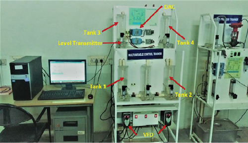
Water is supplied to the four tanks from the sink through two positive displacement pumps P1 and P2, which are regulated by two Variable Frequency Drives (VFD). Pump P1 feeds water to tank 1 and tank 4 through a three-way valve, where water splits into a desired fraction γ_1. Likewise, Pump P2 feeds tank 2 and tank 3 through another three-way valve, where water splits into another fraction γ_2. Through the flow damper, outlet water of tank 3 and tank 4 serves as a second inlet to tank 1 and tank 2, respectively. At last, outlets of tank 1 and tank 2, through flow dampers, return back to the sink. The water level two tanks h1 and h2 at the bottom are measured using level transmitters. The measured signals from level transmitters are connected to Multifunction I/O & NI-DAQMX, which is connected to the computer through USB ports. The process variables h1 and h2 are controlled through a dual loop PID controller, where the controller output is fed to the two variable frequency drives (VFD) which in turn gives signal to the pumps P1 and P2 and vary the water flow rate F1 and F2 discharging through the pumps. The experiment is conducted for the minimum phase operation of the quadruple tank process. Table 1 shows the QTP Experimental Setup Specifications. Figure 2 shows the workflow diagram of QTP experimental setup of proposed RT-QTP and SVM-QTP models through regression technique.

Figure 2. Workflow diagram of QTP experimental setup of proposed RT-QTP and SVM-QTP models through regression technique.

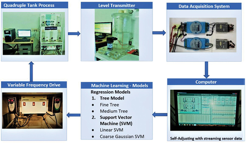
Table 1. QTP Experimental Setup Specifications.

Inner diameter of all four tanks	9.2cm
Cross sectional area of all four tanks	A1, A2, A3, A4=66.47cm2
Maximum height of all four tanks	26.5cm
Maximum flow rate of each pump	F1, F2=55.57LPH
Inner diameter of outlet pipes of all four tanks	1.2cm
Cross sectional area of outlet pipes of all four tanks	a1, a2, a3, a4=1.13cm2

In the proposed workflow, two three-way valves are adjusted to minimum phase condition by fixing the γ₁ and γ₂ values as 1 < γ₁+γ₂<2. As a result, the lower two tanks receive more water when compared to the upper two tanks. Furthermore, flow dampers at the outlet of each tank are adjusted, so that 80–90% of maximum height of water in each tank is maintained, when both the pumps are operated at maximum flow rate. In initial step, both the pumps are set to run manually and provide maximum flow rate.

In the second step, once the steady state condition is reached, the input current to the VFD drive controlling Pump P1 is kept constant for maximum flow rate and the input current to the VFD drive controlling Pump P2 is decreased from maximum to minimum in the step-wise manner. In third step, process is allowed to reach the new steady state value. In the fourth step, input to Pump P1 is decreased to 20% from maximum and Pump P2 values are again varied from maximum to minimum as initial step. Step three and four are repeated to get all possible combinations of inputs. The corresponding input-output streaming data are recorded with the help of data logging system in the software.

Mathematical model of QTP for proposed RT-QTP and SVM-QTP models

Machine learning algorithms optimize the performance criterion of QTP using acquired data. In this paper, we analyzed the performance of proposed algorithms such as RT-QTP and SVM-QTP for continuous streaming data conditions through regression modeling. Existing ML technique for QTP model and performance reduces due to different ambient environment conditions such as ambient temperature and tube condition change. The real time data collected from the laboratory setup is imported into regression learner app in MATLAB software. Before implementing RT-QTP and SVM-QTP, data pre-processing is performed in the data and removes for improving the accuracy of the model.

Regression trees

A regression tree is constructed in almost the same manner as a classification tree, except that the impurity measure that is appropriate for classification is replaced by a measure appropriate for regression [15]. Let us say for node m, X_m is the subset of X reaching node m; namely, it is the set of all x ϵ X satisfying all the conditions in the decision nodes on the path from the root until node m. We can define

$b_m\left(x\right)=\left\{\begin{array}{c}1ifx\in X_m:xreachesnodem\\ 0otherwise\end{array}\right.$

In regression, the goodness of a split is measured by the mean square error from the estimated value. Let us say g_m is the estimated value in node m.

$E_m=\frac{1}{N_m}\sum _t(r^t-g_m{)}^2{b}_m(x^t)$

Where $N_m=\left|X_m\right|=\sum _t{b}_m\left(x^t\right)$

In a node, we use the mean (median if there is too much noise) of the required outputs of instances reaching the node.

Support vector machine regression

SVMs belong to the class of supervised learning algorithms in which the learning machine is given a set of inputs with the associated output values. SVMs construct a hyperplane that separates two classes, while doing so, the SVM algorithm tries to achieve maximum separation between the classes. Separating the classes with a large margin minimizes a bound on the expected generalization error. A “minimum generalization error” means that when new input data arrives for classification, the chance of making an error in the prediction based on the learned classifier will be minimum.

Existing model of QTP model

Differential equation model

Differential equation model is used to describe the dynamics of any system. It relates one or more unknown functions and their derivatives in the equation. The function represents the physical quantity and the derivatives represent their rate of change with respect to time. Mathematical model of systems can be represented with set of mathematical equations. The derived models are useful for analysis and design of systems. Here, differential equation model is a time domain mathematical model of QTP. Applying the mass balance equation and Bernoulli’s law, the mathematical model of QTP is written as Eq (1(1) $\frac{d{h}_1}{dt}=-\frac{a_1}{A_1}\sqrt{2g{h}_1}+\frac{a_3}{A_1}\sqrt{2g{h}_3}+\frac{{\gamma }_1.k_1}{A_1}{V}_1$(1) ):

(1) $\frac{d{h}_1}{dt}=-\frac{a_1}{A_1}\sqrt{2g{h}_1}+\frac{a_3}{A_1}\sqrt{2g{h}_3}+\frac{{\gamma }_1.k_1}{A_1}{V}_1$(1)

(2) $\frac{d{h}_2}{dt}=-\frac{a_2}{A_2}\sqrt{2g{h}_2}+\frac{a_4}{A_2}\sqrt{2g{h}_4}+\frac{{\gamma }_2.k_2}{A_2}{V}_2$(2)

(3) $\frac{d{h}_3}{dt}=-\frac{a_3}{A_3}\sqrt{2g{h}_3}+\frac{(1-{\gamma }_{2)}.k_2}{A_3}{V}_2$(3)

(4) $\frac{d{h}_4}{dt}=-\frac{a_4}{A_4}\sqrt{2g{h}_4}+\frac{(1-{\gamma }_{1)}.k_1}{A_4}{V}_1$(4)

The above equations represent the mass flow dynamics for the four tanks. The nominal values of the parameters K₁, K₂, ${\gamma }_1,{\gamma }_2$are taken as K₁, K₂ − 4.43, ${\gamma }_1,{\gamma }_2-0.7$, g-981 Cm/s².

State space model

A state-space representation is a mathematical model of a physical system as a set of input, output and state variables related by first-order differential equations. State variables x(t) can be reconstructed from the measured input-output data, but are not themselves measured during an experiment. Output variables values depend on the values of the state variables. It is represented in the matrix form and it provides a convenient way to model and analyze systems with multiple inputs and outputs. The most general state-space representation of a linear system is written as

(5) $\dot{x}\left(t\right)=Ax\left(t\right)+Bu\left(t\right)$(5)

(6) $y\left(t\right)=Cx\left(t\right)+Du\left(t\right)$(6)

State space model of the quadruple tank process is obtained through the differential equation model. First, the differential equation is formed as the SIMULINK block diagram with MATLAB. LINMOD function, the state space model is obtained. LINMOD computes a linear state-space model by linearizing each block in a model individually. State space model obtains linear model from system of ordinary differential equations described as Simulink models. Furthermore, Inputs and outputs are denoted in Simulink block diagrams using Inport and Outport blocks. The LINMOD algorithm uses preprogrammed analytic block Jacobians for blocks, which should result in more accurate linearization than numerical perturbation of block inputs and states.The continuous time linear state space model is obtained around the operating point such as h1 = 7.538, h2 = 5.719, h3 = 0.3482, h4 = 0.7841 and u0 = 33.34;22.22

The linearized State-Space Model of the QTP for the above operating point is obtained as below.

$A=\left[\begin{array}{cccc}-0.1371& 0& 0.7281& 0\\ 0& -0.1574& 0& 0.4852\\ 0& 0& -0.6380& 0\\ 0& 0& 0& -0.4252\end{array}\right]$

$B=\left[\begin{array}{cc}0.0468& 0\\ 0& 0.0468\\ 0& 0.0200\\ 0.0200& 0\end{array}\right]$

$C=\left[\begin{array}{cccc}1& 0& 0& 0\\ 0& 1& 0& 0\\ 0& 0& 1& 0\\ 0& 0& 0& 1\end{array}\right]$

Performance indices for proposed RT-QTP and SVM-QTP evaluation

The proposed model such as RT-QTP and SVM-QTP are analyzed using the performance indices such as RMSE, R-Squared, MSE, MAE and prediction speed is considered. Root mean squared error (RMSE) is the square root of the mean of the square of all of the error. RMSE is an excellent general-purpose error metric for numerical predictions and Eq (5(5) $\dot{x}\left(t\right)=Ax\left(t\right)+Bu\left(t\right)$(5) ) shows the RMSE.

(7) $RMSE=\sqrt{\frac{1}{n}{\sum }_{I=1}^n{\left(s_i-O_i\right)}^2}$(7)

where O_i - represents the observations, S_i- predicted values of a variable, and n – the number of observations available for analysis. R-squared (R²) is a statistical measure that represents the proportion of the variance for a dependent variable. Whereas correlation shows the strength of the relationship between an independent and dependent variable. Eq (6(6) $y\left(t\right)=Cx\left(t\right)+Du\left(t\right)$(6) ) shows the R-square calculation.

(8) $R^2=1-\frac{RSS}{TSS}$(8)

R²- Coefficient of determinations- Sum of squares of residuals – Total sum of squares

The mean squared error (MSE) shows how close a regression line is with set of points. MSE does this by taking the distances from the points to the regression line (these distances are the “errors”) and squaring them. The squaring is necessary to remove any negative signs. It also gives more weight to larger differences. The lower the MSE, the better the forecast as shown in Eq (7(7) $RMSE=\sqrt{\frac{1}{n}{\sum }_{I=1}^n{\left(s_i-O_i\right)}^2}$(7) )

(9) $MSE=\frac{1}{n}{\sum }_{i=1}^n(Y_i-{\widehat{Y_i)}}^2$(9)

where n - number of data points, Y_i - Observed Values, $\widehat{Yi}$ - Predicted Values. MAE – The Mean Absolute Error is the average of all absolute errors.

(10) $MAE=\frac{1}{n}{\sum }_{i=1}^n\left|x_i-x\right|$(10)

Where n – number of errors, $\left|x_i-x\right|$ – absolute errors

Results and analysis

RT-QTP and SVM-QTP analyzed through each trained model and depicted as in Figure 3. Figure 3 shows the Response Vs Record number, Predicted Response Vs True Response and Residuals Vs True Response of h1 of proposed RT-QTP. In Fine Tree Model, h1 response of Tank 1 is plotted. Figure 3(a) shows the dataset points of true values and predicted values. The corresponding points of both the curves are close to each other for a good regression performance. Figure 3(b) shows the performance of the regression task. The data points (blue) lie along the black curve (perfect prediction) show that the true and predicted values are close to each other. The more points are aligned along the perfect prediction line, says that the prediction is better.

Figure 3. Regression Tree-Quadruple Tank Process (RT-QTP) Model responses for water level (h1) in Tank-1.

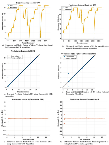
Figure 3(c) shows the residual plot between residual (predicted-true) and predicted targets. The plot shows a random pattern of points. For better regression performance, this residual plot should exhibit a random pattern and the points should be symmetrically distributed along the y = 0 line. These plots are vital for visualization of the quality of regression among the true and predicted targets. How the data points are close or far to each other. In Medium Tree Model response is shown in Figure 3. The h1 response of Tank 1 is plotted. Figure 3(d) shows the response of true and predicted values, which are close to each other. Figure 3(e) shows the scattered points, which are close to the diagonal line and proves exceedingly small errors. Figure 3(F) shows the residuals are located around y = 0 line. Residuals are almost symmetrically distributed around 0. No outliers are found. A clear linear pattern appears in the residuals.

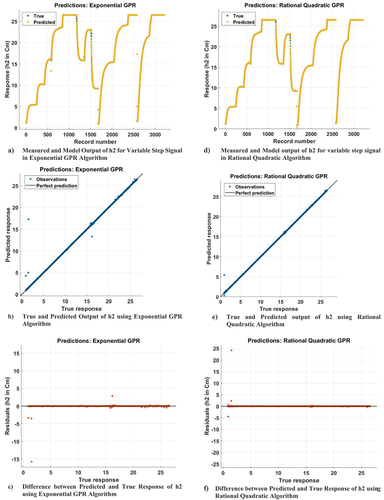
Fine Tree Model response plot is shown in Figure 4; the h2 response of Tank 2 is plotted. Figure 4(a) shows the true and predicted values are perfectly plotted one above the other. Figure 4(b) shows the performance of the regression task. The data points (blue) lie along the black curve (perfect prediction), showing that the true and predicted values are lying exactly upon the prediction line. The more points are aligned along the perfect prediction line, and proves as prediction is better. In Figure 4(c) the points are closely located around the y = 0 line, exhibiting the model is a perfect one. Medium Tree Model response is shown in Figure 4. The h2 response of Tank 2 is plotted. Figure 4(d) shows the response of true and predicted values lying close together. Figure 4(e) shows the scattered points are nearer to the diagonal line, and errors are minimum. In Figure 4(F) the residuals are located around y = 0 line. Residuals are nearly distributed around 0. Few outliers are found at the right-hand side end.

Figure 4. Regression Tree- Quadruple Tank Process (RT-QTP) Model responses for water level (h2) in Tank-2.

Support vector machine (SVM) models

Support Vector Machines algorithm acknowledges the presence of nonlinearity in the data and provides a proficient prediction model. The objective of a support vector machine algorithm is to find a hyperplane in an n-dimensional space that distinctly classifies the data points. The data points on either side of the hyperplane that are close to the hyperplane are called Support Vectors. The vector influences the position and orientation of the hyperplane and builds the SVM. In the Linear SVM Model of Figure 5. The h1 response of Tank 1 is plotted. Figure 5(a) shows the true and predicted values are closer to each other. In Figure 5(b) the observation points are scattered almost nearer the perfect prediction line.

Figure 5. Support Vector Machine- Quadruple Tank Process (SVM-QTP) Model responses for water level (h1) in Tank-1.

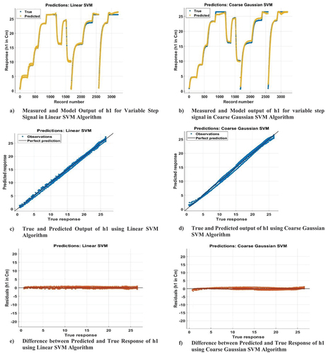
In the Coarse Gaussian SVM Model of Figure 5 the h1 response of Tank 1 is plotted. Figure 5(d) shows the true and predicted values plotted nearer to each other. In Figure 5(e) the observation points are scattered around the perfect prediction line and never like the Fine Tree and Medium Tree. In the Linear SVM Model of Figure 6, the h2 response of Tank 2 is plotted. Figure 6(a) shows the true and predicted values are closer to each other. In Figure 6(b) the observation points are scattered almost nearer the perfect prediction line. In the Coarse Gaussian SVM Model of Figure 6 the h2 response of Tank 2 is plotted. Figure 6(d) shows the true and predicted values plotted nearer each other. In Figure 6(e) the observation points are scattered around the perfect prediction line and never like the Fine Tree and Medium Tree.

Figure 6. Support Vector Machine- Quadruple Tank Process (SVM-QTP) Model responses for water level (h2) in Tank-2.

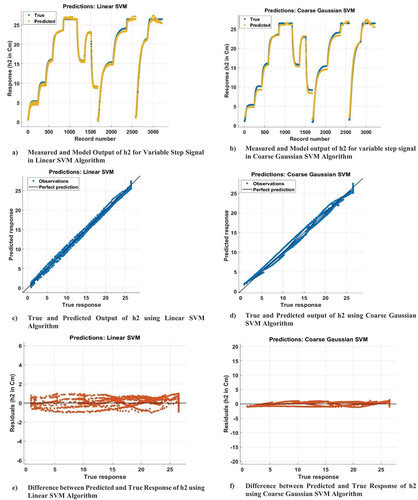
In Table 2 Fine Tree algorithm applied for h1 prediction and R² has value of 0.99 which is remarkably close to the best possible score of 1.0. RMSE (Root Mean Squared Error) is about 0.53, which proves that the predicted values are close to the true values. The mean squared error (MSE) value is 0.28 and the mean absolute error (MAE) is 0.07. The predicted value is almost equal to the true values. Using the Medium Tree algorithm for h1 prediction, the MSE value is 0.27 which is less compared to Fine Tree model. The MAE is about 0.09 and proves as best model. RT-QTP model predicts the response accurately, when compared to traditional modeling. Fine Tree algorithm for h2 prediction performance shows RMSE value as 0.52, R² value as 1, MSE as 0.27 and MAE value as 0.07. Using the Medium Tree algorithm for h2 prediction, the model shows the RMSE value as 0.49, R² value as 1, MSE value as 0.24 and the MAE is 0.07. The prediction speed is approximately 51,000 obs/sec.

Table 2. Performance comparison of RT-QTP, SVM-QTP Models with conventional model performance.

Performance Comparison of Machine Learning Models and Conventional Models for Liquid Level h1
ML Regression Learner	Tank Height	RMSE	R-Squared	MSE	MAE	Prediction Speed (obs/sec)	Training Time (sec)
Fine Tree	H1	0.53	0.99	0.28	0.07	~21000	0.70
Medium Tree		0.52	1	0.27	0.09	~21000	0.51
Linear SVM		0.85	0.99	0.73	0.53	~47000	70.70
Coarse Gaussian SVM		0.79	0.99	0.62	0.46	~53000	0.65
Differential Equation Model		0.90	-	0.82	0.10	-	-
State-Space Model		0.90	-	0.81	0.10	-	-
Performance Comparison of Machine Learning Models and Conventional Models for Liquid Level h2
Fine Tree	H2	0.52	1	0.27	0.07	~53000	2.65
Medium Tree		0.49	1	0.24	0.07	~170000	0.77
Linear SVM		0.43	1	0.18	0.33	~120000	2.11
Coarse Gaussian SVM		0.70	0.99	0.49	0.50	~190000	0.48
Differential Equation Model		1.02	-	1.04	0.11	-	-
State-Space Model		0.96	-	0.92	0.10	-	-

Support Vector Machine (SVM) algorithm is applied for h1 prediction, The RMSE value is 0.85. The R² value is 0.99 and proves as better model. The MSE and MAE values are 0.73 and 0.53 and considerably more, when compared to the Fine and Medium Tree Performances. At the same time, the prediction speed is approximately 47,000 obs/sec, which is better than Fine and Medium Tree Prediction Speeds per second. RMSE value is 0.65, which is slightly higher than the other models. R² value is 0.99, and prove the model is better. MSE and MAE values are 0.42 and 0.37, which are slightly higher compared to other models. Simultaneously, the prediction speed is approximately 220,000 obs/sec, which is better when compared to the Prediction Speeds of other models. The RMSE value is 0.45. The R² value is 1 and model proves as better for prediction. MSE and MAE values are 0.20 and 0.36, which are slightly more, when compared to Fine and Medium Tree algorithms. The prediction speed is approximately 230,000 obs/sec. The RMSE value is 0.69, which is slightly higher than the other models. The R² value is 0.99 and the model is better. The MSE and MAE values are 0.48 and 0.50, which are slightly higher compared to other models. The prediction speed is approximately 220,000 obs/sec. The Performance analysis of Regression Based QTP modeling techniques are presented and compared, the degree of prediction accuracy and generalization capabilities with traditional techniques applied to quadruple tank process. In the prediction of water level h1, RT-Medium Tree Algorithm shows a minimum RMSE, MSE and MAE value. Moreover, Linear SVM model shows a better prediction of water level for h2 compared to the other models. Table 3 shows the comparison of proposed and existing models implemented in our QTP test bed.

Table.3. Comparison of Proposed and Existing algorithms for QTP system.

S.No	Algorithm	RMSE in prediction of liquid level h1	RMSE in prediction of liquid level h2
1	Tree Models – Fine Tree & Medium Tree (Proposed)	0.53 & 0.52	0.52 & 0.49
2	SVM Models – Linear SVM and Coarse Gaussian (Proposed)	0.85 & 0.79	0.43 & 0.70
3	Differential equation model [6]	0.90	1.02
4	State space model [6]	0.90	0.96
5	Fuzzy [6]	0.89	0.87

Conclusion

In this paper, the mathematical modeling of Quadruple Tank Process (QTP) is first derived in the conventional methods known as the differential equation model and state-space model. Then using the real time dataset, the regression tree-based models are developed using Machine Learning Application in MATLAB. We assess the prediction accuracy in terms of R², RMSE and MAE and compare the results of SVM and Tree models. Results indicate that the machine learning models provide a better prediction. This work is carried out to address the difficulties involved in the mathematical modeling of multi-loop systems having high interactions between their inputs and outputs. We conducted experiments with the real-time laboratory setup dataset and developed prediction models with selected machine learning algorithms and the accuracy of the predicted models are compared in Tab 4. This suggests that both Tree and SVM models are extremely accurate in predicting the liquid levels h1 and h2 compared to the conventional modeling techniques. Using Machine Learning technique, only a few numbers of features are of key importance in our models and with those few features, we can make highly accurate predictions for the given dataset. Our study provides an efficient pipeline for similar performance prediction and evaluation of multi-input multi-output systems. In future, deep learning algorithms can be applied to improve the accuracy for other types of liquid.

Availability of Data and Materials

The datasets generated during and/or analyzed during the current study are available from the corresponding author on reasonable request.

Ethical Approval

I will conduct myself with integrity, fidelity, and honesty. I will openly take responsibility for my actions, and only make agreements, which I intend to keep. I will not intentionally engage in or participate in any form of malicious harm to another person or animal.

Disclosure statement

No potential conflict of interest was reported by the authors.

Additional information

Funding

The authors received no financial support for the research, authorship, and publication of this article.

References

- Aftab, R. A., S. Zaidi, M. Danish, S. M. Adnan, K. B. Ansari, and M. Danish. 2021. Support vector regression-based model for phenol adsorption in rotating packed bed adsorber. Environmental Science and Pollution Research 1 (1):452–622. doi:10.1007/s11356-021-14953-9.
- Biswajit, D., and S. J. Mija. 2021. Emotional learning based controller for quadruple tank system - an improved stimuli design for multiple set-point tracking. IEEE Transactions on Industrial Electronics 68 (issue. 11). doi: 10.1109/TIE.2020.3038083.
- Chuongvo, L., L. V. T. Nguyen, and M. Lee, “Fractional order modeling and control of a quadruple-tank process,” in Proceedings of 2020 5th International Conference on Green Technology and Sustainable Development, GTSD, Ho Chi Minh City, Vietnam, pp. 334–39, 2020. doi:10.1109/GTSD50082.2020.9303059
- Doguş Universitesi Istanbul, International symposium on innovations in intelligent systems and applications 2011.06.15-18 Istanbul, and INISTA 2011.06.15-18 Istanbul, International Symposium on Innovations in Intelligent Systems and Applications (INISTA), Istanbul, Turkey, 2011.
- Govinda Kumar, E., B. Shiva Ram, U. B. Deepak, and G. Sabarinathan. 2018. The quadruple tank process with an interaction: A mathematical model. International Journal of Engineering & Technology 7 (24):172–76.
- Hipni, A., A. E. Shafie, A. Najah, O. A. Karim, A. Hussain, and M. Mukhlisin. 2013. Daily forecasting of dam water levels: Comparing a support vector machine (svm) model with adaptive neuro fuzzy inference system (anfis). Water Resources Management 27 (10):3803–23. doi:10.1007/s11269-013-0382-4.
- Jayaprakash, J., T. Senthil Rajan, and T. H. Babu. 2014. Analysis of modelling methods of quadruple tank system. International Journal of Advanced Research in Electrical, Electronics and Instrumentation Engineering 3 (8):11552–65. doi:10.15662/ijareeie.2014.0308070.
- Johansson, K. H. 2000. The quadruple-tank process: A multivariable laboratory process with an adjustable zero. IEEE Transactions on Control Systems Technology 8 (3):456–65. doi:10.1109/87.845876.
- Kirchgassner, W., O. Wallscheid, and J. Bocker. 2021. Data-driven permanent magnet temperature estimation in synchronous motors with supervised machine learning: A benchmark. IEEE Transactions on Energy Conversion 36 (3):2059–67. doi:10.1109/TEC.2021.3052546.
- Lee, J., I. Kyoung, J. Pil Heo, Y. Park, Y. Lim, D. Hyun Kim, Y. Lee, and D. Ryook Yang. 2017. A simple method to make the quadruple tank system near linear. Korean Chemical Engineering Research 55 (6):767–70.
- Lee, J., W. Wang, F. Harrou, and Y. Sun. 2020. Wind power prediction using ensemble learning-based models. IEEE Access 8 (2):61517–27. doi:10.1109/ACCESS.2020.2983234.
- Nguyen, T. T., and H. T. Le, “Water level prediction at tich-bui river in Vietnam using support vector regression,” International Conference on Machine Learning and Cybernetics (ICMLC), Kobe, Japan, 2019. doi:10.3390/w14101617
- Sapitang, M., W. M. Ridwan, K. F. Kushiar, A. N. Ahmed, and A. E. Shafie. 2020. Machine learning application in reservoir water level forecasting for sustainable hydropower generation strategy. Sustainability 12 (15):6121–30. doi:10.3390/su12156121.
- Sebastian, D., and F. Esquembre, “The quadruple tank process: An interactive tool for control education,” 7th European Control Conference, ECC 2003, Cambridge, UK, September 1-4, IEEE, pp. 3267–72, 2003. doi: 10.23919/ECC.2003.7086543.
- Subramanian, S., G. B. Chidhambaram, and S. Dhandapani. 2021. Modeling and validation of a four-tank system for level control process using black box and white box model approaches. IEEJ Transactions on Electrical and Electronic Engineering 16 (2):282–94. doi:10.1002/tee.23295.
- Suja, R., M. Malar, and T. Thyagarajan. 2009. Modeling of quadruple tank system using soft computing techniques. European Journal of Scientific Research 29 (2):249–64.
- Tousi, A., and M. Lujan. 2022. Comparative analysis of machine learning models for performance prediction of the spec benchmarks. IEEE Access 10 (4):11994–2011. doi:10.1109/ACCESS.2022.3142240.
- Wang, Q., and S. Wang. 2020. Machine learning-based water level prediction in lake erie. Water 12 (10):2654–60. doi:10.3390/w12102654.
- Zhao, W., H. Wang, and Z. Wang. 2011. Groundwater level forecasting based on support vector machine. Applied Mechanics and Materials 44-47 (1):1365–69. doi:10.1016/j.neucom.2022.03.014.
- Zhu, M., A. Hahn, Y. Q. Wen, and W. Q. Sun. 2019. Optimized support vector regression algorithm- based modeling of ship dynamics. Applied Ocean Research 90 (6):101842–50.