Toward Data-Driven and Multi-Scale Modeling for Material Flow Simulation: Characteristic Analysis of Modeling Methods

ABSTRACT

Material flow simulation is a powerful tool to realize efficient operations in complicated production systems such as high-mix and low-volume production. Nevertheless, great effort and expertise are necessary to construct accurate simulation models. We have proposed a semi-automatic modeling approach designated as data-driven and multi-scale modeling. The approach combines various modeling methods to maximize the simulation accuracy. This article introduces the proposed method and presents the experimentally obtained results for simple production systems to examine the characteristics of modeling methods based on queue models or machine learning models. The results of computational experiments indicate that the superiority and inferiority of modeling methods depend on the complexity of the system and the background knowledge about the activity configuration in the system.

Introduction

Recently, production systems such as high-mix and low-volume production have become more complicated due to the diversification of market needs. To achieve efficient operations in such systems, cyber-physical production systems (CPPS) and digital twin are attracting attention (Monostori 2014). For these concepts, material flow simulation is an important tool to predict future production (Rosen et al. 2015). However, in practice, building accurate simulation models requires a great deal of effort and expertise. This difficulty hinders the realization of the CPPS/digital twin concept in the industry, and automatic modeling methods are demanded. In recent years, more data are obtainable from production systems by virtue of the advance of IoT devices. Additionally, machine learning (ML) techniques are advancing remarkably. ML techniques enable us to identify system behavior from the data and enable us to make models with different scales such as production processes and entire systems. This capability is expected to be useful because complete mimicking of an actual system is often difficult, and it is required to abstract the system according to available data. Given the background presented above, we propose a data-driven and multi-scale modeling approach that semi-automatically constructs accurate simulation models by combining various modeling methods. In this paper, we verify the superiority and inferiority of modeling methods through computational experiments in order to consider the course of development of the proposed approach.

Challenges in Material Flow Simulation Modeling

General Modeling Process for Material Flow Simulation

Material flow is the description of the transportation of materials. Material flow simulation is a widely used technology that enables us to predict the movement of materials in discrete systems such as production and logistics systems. Material flow simulation is mainly utilized to support human decision making in production system design and production planning (Hoellthaler et al. 2019; Lechner et al. 2023).

Production systems consist of a set of processes in which materials are processed, assembled, stored, etc. Therefore, a material flow simulation model is generally described by a set of queue models that express a production process. A general modeling process is as follows. First, the model configuration parameters such as scope and granularity of model are defined so that the purpose of simulation use is achieved. Next, the data necessary to define the model are prepared. Queue models consist of various activities such as dispatching, machining, and setup. Table 1 shows an example of typical activities, their behavior, and required information to determine the behavior. It is necessary to collect and/or create various data to define the respective behaviors associated with those activities. Then, the model is implemented on simulation software using the prepared data. Finally, the model is validated. The simulation accuracy is evaluated by the comparison of simulation results with the actual production log. The model is reviewed in a trial-and-error manner. Not only activity behavior but also the model configuration is sometimes revised until the required degree of accuracy is achieved. The modeling process above consists of many manual tasks. Moreover, it depends on the modeler’s subjective decisions. Therefore, the automation of modeling process is important to widely utilize material flow simulation.

Table 1. An example of activities in a queue model.

Activity	Activity behavior	Required information
Dispatching	Select jobs to be processed next from jobs in a queue.	Job dispatching rule
Resource assignment	Select resources (e.g., machine, worker) to be used for the next jobs.	Resource assignment rule
Setup	Determine whether setup operations are required based on the difference of product type between the previous job and successive job processed by the resources, then occupy the resources for a predefined time of setup operations if needed.	Setup operation occurrence conditions and setup time for each condition
Machining	Occupy the resources for a predefined time of machining operations.	Machining time for each product type
Routing	Move jobs to the queue of the next process.	Process route for each product type

Related Works and Challenges

Regarding automatic modeling for material flow simulation, most existing research leverages data models and system architectures to automatically generate simulation programs from data (Barlas and Heavey 2016). For instance, Kirchhof et al. proposed a method by which simulation objects representing production processes are defined in advance. Then those objects are combined based on MES data (Kirchhof 2016). Steinbacher et al. provided an ontology to generate material flow simulation models for logistics systems (Steinbacher et al. 2023). Also, Henkenjohann et al. proposed standard modules in production for material flow simulation to simplify model implementation into the simulation environment (Henkenjohann et al. 2021). These studies are helpful to reduce the effort for model implementation.

Some studies have examined the improvement of simulation accuracy. For instance, Karnok et al. proposed a method that estimates process routes and operation time from production logs (Karnok and Monostori 2011). Popovics et al. proposed a method to construct a response model of a conveyor system from PLC programs (Popovics and Monostori 2013). Nagahara et al. proposed a method to identify dispatching rules using ML techniques (Nagahara, Sprock, and Helu 2019). They also proposed a method that calibrates parameters in a simulation model to maximize accuracy (Nagahara et al. 2020). May et al. utilized process mining techniques and convolutional nerual networks to identify process routing and resource assignment rules from production log data (May et al. 2024). The methods above are useful to reduce the effort for data preparation to determine the behavior of activities in queue models. In addition, ML-based methods that directly express the input–output relation of the system have been proposed. For instance, Lingitz et al. proposed a method that predicts production lead time using artificial neural networks, random forest, etc. (Lingitz et al. 2018). Since this method do not use queue models, it enables us to reduce the effort required to define activity configuration in queue models and preparing data for each activity.

As explained above, various modeling methods are proposed to identify the behaviors of a production system. However, what kind of modeling method is suitable for a specific system remains unclear. In practice, the activities in actual production system are different for each system, and it is often difficult and time-consuming to comprehend all activities in the system and describe them in simulation models. Therefore, it is important to use modeling methods depending on the characteristics and available information of target system. Furthermore, in a production system with multiple processes, the activity configuration and activity behavior are different for each process. Therefore, the most appropriate modeling method can be different for each process, and it is important to utilize multiple modeling methods to build an accurate model of entire system. From the above point of view, we proposed a data-driven and multi-scale modeling approach to optimize the configuration of a simulation model by combining various modeling methods in our earlier study (Nagahara et al. 2022). In this paper, we focus on production systems with single process which has different activities. We compare the prediction capability of models obtained by different modeling methods to investigate the superiority and inferioirty of modeling method as a fundamental study to verify the usefulness of the proposed approach.

Proposed Method

Classification of Modeling Methods

In this chapter, the modeling approach proposed in our earlier study is briefly reviewed to complement the discussions presented in the following chapters.

Table 2 describes the proposed classification of modeling methods. The modeling methods are classified from viewpoints of two kinds: model scale such as the activity/process/system scale; and model type such as a white/black/gray box model. Here, model scale indicates the scope of models. Activity-scale models refer to models that focus on individual activities such as dispatching, machining, etc. Process-scale models indicate models that focus on a process, and system-scale models indicate models that focus on a system composed with multiple processes.

Table 2. Classification of modeling methods.

Modeling method	Model scale	Model type	Definition
Activity WBM	Activity	White box	Describe the behavior of activity explicitly and deductively based on background knowledge.
Activity BBM		Black box	Build an ML model that implicitly express the input–output relationship of the activity from activity log.
Process BBM	Process	White box	Build a queue model in which all activities are expressed by activity WBM and the connections between activities is also explicitly described.
Process BBM		Black box	Build an ML model that directly predict the process output from input.
Process GBM		Gray box	Build a queue model in which sum/all activities are expressed by activity BBM and the connections between activities is explicitly described.
System WBM	System	White box	Build a model in which all processes are expressed by process WBM (used in general simulation software).
System BBM		Black box	Build an ML model that directly predict the system output from input.
System GBM-1		Gray box	Build a model in which some/all processes are expressed by process GBM/BBM.
System GBM-2			Build a model in which any subsystem, which is composed with some processes, in the entire system is expressed by system BBM.

As the activity scale models, activity white box model (activity WBM) and activity black box model (activity BBM) are defined. Activity WBM is a model in which the activity behavior is defined explicitly and deductively. Activity BBM is an ML-based model that inductively expresses the input–output relation of the activity. As the process scale models, process WBM, process BBM, and process gray box model (process GBM) are defined. Process WBM is a queue model composed with activity WBMs. Process BBM is an ML-based model that inductively expresses the input–output relation of the process. Process GBM is a queue model in which some or all activities are expressed by activity BBM. On the system scale, system WBM, system BBM, system GBM-1, and system GBM-2 are defined. System WBM is composed with process WBMs. System BBM is an ML model that expresses the input–output relation of the system. System GBM-1 is a model in which some or all processes are expressed by the process GBM/BBM. System GBM-2 is a model by which any subsystem in the entire system is expressed by system BBM.

Data-Driven and Multi-Scale Modeling

Based on the classification above, the data-driven and multi-scale simulation modeling shown in Figure 1 has been proposed. The proposed method aims at deriving an accurate simulation model by combining various modeling methods. The notations of W/G/B in Figure 1 respectively represent WBM/GBM/BBM on an arbitrary scale (activity/process/system). As shown in Models (a), (b), and (c) in Figure 1, various model configurations can be considered for a certain system. The proposed method generates multiple model configurations by integrating and dividing the processes and activities (Figure 1(1)). Then, according to the input–output requirements for the simulation use, the parameters in each model are calibrated to predict changes in the output accurately with respect to changes in the input (Figure 1(2)). Finally, the most accurate model is selected (Figure 1(3)). This method is a data-driven method that selects the optimal model configuration based on simulation accuracy. Furthermore, this method is a multi-scale modeling method that combines models of different scales.

Figure 1. Schematic view of the proposed modeling approach.

The requirements for simulation input and output depend on the purpose of simulation use and various purposes of simulation use can be supposed. For instance, for due date reply, it is important to predict the completion date-time of each job from the arrival date-time of each job as simulation input. On the other hand, if simulation is used for the design of production system, simulation is required to predict the throughput of production system from the number of production resources such as machines. The accuracy of simulation should be evaluated based on the perspective above. In other words, the requirement for simulation models is to accurately predict the change in output according to the change in input. In the proposed method, therefore, simulation models are calibrated to minimize the prediction error in output in Figure 1(2).

Hereafter, it is assumed that the input and output of simulation are arrival date-time and completion date-time of each job respectively to concretely describe the detail of the proposed method. In the case that we divide the entire system into subsystems and construct subsystem models as shown in Figure 1, subsystem models are connected by utilizing job completion date-time of a subsystem model as job arrival date-time of other subsystem models. Therefore, it is important to consider models which predict job completion date-time from job arrival date-time. Since predicting job completion date-time from job arrival date-time is synonymous with predicting job lead time, the purpose of simulation is defined as job lead time prediction hereafter.

As mentioned above, there are various activities such as dispatching, setup, and machining in production systems. If the activity configuration of target system and the behavior of all activity are known, system WBM can be built based on the information above. On the other hand, if the behavior of some activities is unknown and the actual log data regarding the input and output of activity behavior (hereafter, we call this data as activity log data), activity BBMs of those activities can be constructed independently of each other using the activity log data and ML techniques. However, if the activity log data are not available, it is necessary to make a model from other data. For instance, in the case that the data regarding start and completion date-time of setup activity for each job are unavailable and the data regarding arrival and completion date-time of each process are available, it is necessary to calibrate models using the latter data. For such cases, we proposed two modeling method; (1) one is to build a GBM by calibrating the parameters which define the behavior of activities in queue models and (2) the other is to build a BBM that directly predict the job completion date-time from job arrival date-time by ML techniques.

As a method for (1), we propose a method that calibrates the parameters in GBMs using particle swarm optimization (PSO) which is a continuous optimization technique. For instance, in the case that a queue model with a machining activity is determined as a process GBM, machining time for product type as the parameters which define the behavior of the machining activity have to be calibrated appropriately for accurate prediction of job lead time. The parameters that need to be calibrated depend on the activity configuration of the model. In this method, the parameter vector $\mathit{X}$, which defines the behaviour of each activity in GBMs, are searched by PSO to minimize the error on job lead time. The objective function $J^{\mathit{GBM}}$ is shown by equation (1)(1) $J^{\mathit{GBM}}=||\mathit{l}{\mathit{t}}^{\mathit{ref}}-\mathit{l}{\mathit{t}}^{\mathit{GBM}}||$(1) .

(1) $J^{\mathit{GBM}}=||\mathit{l}{\mathit{t}}^{\mathit{ref}}-\mathit{l}{\mathit{t}}^{\mathit{GBM}}||$(1)

Here, $\mathit{l}{\mathit{t}}^{\mathit{ref}}$ and $\mathit{l}{\mathit{t}}^{\mathit{GBM}}$ are, respectively, vectors of the lead time in the target system and GBM. $\mathit{l}{\mathit{t}}^{\mathit{GBM}}$ corresponds to the predicted lead time in the GBM applying the values of parameter vector $\mathit{X}$. As a method for the update of $\mathit{X}$, R-best model proposed by Choi et al. is used (Choi, Ohmori, and Yoshimoto 2011). $\mathit{X}$ is updated by the following equations:

(2) ${\mathit{X}}_{\mathit{i}}^{\mathit{k}+1}={\mathit{X}}_{\mathit{i}}^{\mathit{k}}+{\mathit{V}}_{\mathit{i}}^{\mathit{k}+1}$(2)

(3) $\begin{array}{c}{\mathit{V}}_{\mathit{i}}^{\mathit{k}+1}=\mathit{w}\times {\mathit{V}}_{\mathit{i}}^{\mathit{k}}+c_1\ast \mathit{rand}()\ast \left(\mathit{gbest}-{\mathit{X}}_{\mathit{i}}^{\mathit{k}}\right)\\ +c_2\ast \mathit{rand}()\ast \left(\mathit{pbes}{\mathit{t}}_{\mathit{i}}-{\mathit{X}}_{\mathit{i}}^{\mathit{k}}\right)\end{array}$(3)

Here, $\mathit{V}$ is called as velocity vector. ${\mathit{X}}_{\mathit{i}}^{\mathit{k}}$ and ${\mathit{V}}_{\mathit{i}}^{\mathit{k}}$ are, respectively, the parameter vector and velocity vector of particle i in generation k. $\mathit{gbest}$ is the parameter vector of the best solution in the search process, and $\mathit{pbes}{\mathit{t}}_{\mathit{i}}$ is the parameter vector of the best solution of particle i in the search process. $\mathit{w}$, $c_1$ and $c_2$ are weighting factors.

As a method for (2), we propose a method that constructs a BBM using ANN (artificial neural network) with N inputs and 1 output. The input of ANN is a feature vector for an arbitrary job, and the output is the predicted lead time of that job. The loss function $J^{\mathit{BBM}}$ is shown by equation (4)(4) $J^{\mathit{BBM}}=||\mathit{l}{\mathit{t}}^{\mathit{ref}}-\mathit{l}{\mathit{t}}^{\mathit{BBM}}||$(4) .

(4) $J^{\mathit{BBM}}=||\mathit{l}{\mathit{t}}^{\mathit{ref}}-\mathit{l}{\mathit{t}}^{\mathit{BBM}}||$(4)

Here, $\mathit{l}{\mathit{t}}^{\mathit{BBM}}$ is a vector of lead time predicted by BBM. Because the lead time of job i depends not only on the arrival date-time of job i but also on product type and the jobs which arrive before and after job i, the inputs of ANN should include such information. Therefore, we define the features of job i as equations (5(5) $x_m^i=\left\{\begin{array}{c}1\mathit{if}\mathit{p}{t}_i=\mathit{m}\\ 0\mathit{otherwise}\end{array}\right.\left(\mathit{m}=1,\dots ,\mathit{M}\right)$(5) ), (6(6) $y_{d,m}^i={\sum }_j{\delta }_{j,d,m}^i\left(\mathit{j}=1,\dots ,\mathit{N};\mathit{d}=-\mathit{D},\dots ,\mathit{D}-1;\mathit{m}=1,\dots ,\mathit{M}\right)$(6) ), and (7(7) $\mathit{where}{\delta }_{j,d,m}^i=\left\{\begin{array}{c}1\mathit{if}\mathit{j}\ne \mathit{i}\mathit{and}\mathit{p}{t}_j=\mathit{mand}\\ \mathit{d}\cdot \mathrm{\Delta D}\le t_j^{in}-t_i^{in}<\left(\mathit{d}+1\right)\cdot \mathrm{\Delta D}\\ 0\mathit{otherwise}\end{array}\right.$(7) ).

(5) $x_m^i=\left\{\begin{array}{c}1\mathit{if}\mathit{p}{t}_i=\mathit{m}\\ 0\mathit{otherwise}\end{array}\right.\left(\mathit{m}=1,\dots ,\mathit{M}\right)$(5)

(6) $y_{d,m}^i={\sum }_j{\delta }_{j,d,m}^i\left(\mathit{j}=1,\dots ,\mathit{N};\mathit{d}=-\mathit{D},\dots ,\mathit{D}-1;\mathit{m}=1,\dots ,\mathit{M}\right)$(6)

(7) $\mathit{where}{\delta }_{j,d,m}^i=\left\{\begin{array}{c}1\mathit{if}\mathit{j}\ne \mathit{i}\mathit{and}\mathit{p}{t}_j=\mathit{mand}\\ \mathit{d}\cdot \mathrm{\Delta D}\le t_j^{in}-t_i^{in}<\left(\mathit{d}+1\right)\cdot \mathrm{\Delta D}\\ 0\mathit{otherwise}\end{array}\right.$(7)

Here, $x_m^i$ and $y_{d,m}^i$ are the features of job i. $\mathit{p}{t}_i$ is the index of product type of job i, thus ${\mathit{x}}^{\mathit{i}}=\left\{x_1^i,x_2^i,\dots ,x_M^i\right\}$ is a one-hot vector that represents the product type of job i. $y_{\mathit{d},\mathit{m}}$ denotes the number of arrival jobs of product type m in a certain period determined by $t_i^{in}$ and parameters D and ΔD. D signifies the number jobs which arrive before and after job i. ΔD is the unit length of the period above. Thus, $y_{\mathit{d},\mathit{m}}$ is a variable which express the features of the job arrival plan.

The methods described above are applicable not only to single process but also to multiple processes. If production log data includes job arrival/completion date-time for each process, system GBM can be constructed by combining process GBM or BBM of each process. Even if only the job arrival date-time in the first process and the job completion date-time in the final process are available in production log data, it is possible to construct a Ssystem GBM or system BBM by the above methods.

Computational Experiments

Purpose of Experiments

The proposed method combines WBM/BBM/GBM to achieve high accuracy. In other words, the proposed method assumes that the superiority of each modeling method depends on the characteristics of target system. The superiority of the modeling method is closely related to the available data and background knowledge. For example, if we know all activities in the target system and their behavior, system WBM achieve high accuracy. If the activities and/or their behavior are partially unknown, system WBM would be inaccurate. However, if the activity log of some activities is available, it is possible to construct activity BBM of them. Understanding the superiority and inferiority of modeling methods is important to consider methods for model configuration optimization.

From the perspectives presented above, we conducted computational experiments to compare process GBM and process BBM for production systems with a single process and a single machine in an earlier study (Nagahara et al. 2022). From that study, we ascertained that process GBM tends to be superior to process BBM if the activity configuration in the actual process is known.

For this research, we conduct additional experiments to complement the above analysis. Specifically, we examine how the complexity of system affects the prediction capability of process GBM and process BBM through the experiments for production system with a single process and multiple machines. Additionally, we examine the generalizability of modeling methods against the change in job arrival frequency.

Experimental Conditions

In this experiment, two virtual production systems are assumed as target production systems: System A and System B in Figure 2. Both System A and B are mixed flow production systems with a single process. System A consists of dispatching and machining activities. System B also has transportation and sequence-dependent setup activities. Transportation time $l_p$ and machining time $d_p$ differ for product type p. Setup time $s_{\mathit{p},\mathit{q}}$ differs for the combination of previous product type p and successive product type q. The dispatching rule is first-in first-out (FIFO).

Figure 2. Experimental conditions: target production system.

For this experiment, process WBMs of System A and B are regarded as actual production system. Specifically, we created 1,000 scenarios in which the arrival date-time $t_i^{in}$ and product type index $\mathit{p}{t}_i$ of job i are set randomly for modeling and validation respectively. Then, the completion date-time $t_i^{out}$ and lead time $\mathit{l}{t}_i$ of job i are calculated for each scenario from simulation results of the process WBMs. In the process WBMs, the values of $l_p$, $d_p$ and $s_{\mathit{p},\mathit{q}}$ are set randomly. In each scenario, the number of product types M is 5 and the number of jobs N is 50. The number of machines is varied to examine the effect of system complexity.

Furthermore, we apply different conditions of the job arrival frequency for modeling and validation datasets to evaluate the generalizability. We introduce a parameter α and set $t_i^{in}$ in each scenario by equations (8(8) $t_i^{in}=t_i^{in\mathrm{itial}}+\mathit{\alpha }\ast \mathit{T}\ast r_i\left(\mathit{i}=1,\dots ,\mathit{N}\right)$(8) ) and (9(9) $\mathit{where}{r}_i\leftarrow \mathit{U}\left[0,1\right],\mathit{T}=\sum _{\mathit{j}=1}^N\left(d_{p{t}_j}+\sum _{\mathit{q}=1}^M{s}_{\mathit{p}{\mathit{t}}_{\mathit{j},\mathit{q}}}/\mathit{M}\right)$(9) ).

(8) $t_i^{in}=t_i^{in\mathrm{itial}}+\mathit{\alpha }\ast \mathit{T}\ast r_i\left(\mathit{i}=1,\dots ,\mathit{N}\right)$(8)

(9) $\mathit{where}{r}_i\leftarrow \mathit{U}\left[0,1\right],\mathit{T}=\sum _{\mathit{j}=1}^N\left(d_{p{t}_j}+\sum _{\mathit{q}=1}^M{s}_{\mathit{p}{\mathit{t}}_{\mathit{j},\mathit{q}}}/\mathit{M}\right)$(9)

In those equations, $t^{\mathit{initial}}$ represents the initial date-time of simulation. The smaller value of α denotes the higher job arrival frequency. The value of α is set randomly from $\mathit{U}\left[{\alpha }_{\mathit{min}},{\alpha }_{\mathit{max}}\right]$ for each scenario. Also, ${\alpha }_{\mathit{min}}$ and ${\alpha }_{\mathit{max}}$ are set for each dataset. Hereinafter, ${\alpha }_{\mathit{min}}$ and ${\alpha }_{\mathit{max}}$ are designated as arrival frequency parameters; also, $\left({\alpha }_{\mathit{min}},{\alpha }_{\mathit{max}}\right)$ for the modeling dataset and validation dataset are described respectively as $\left({\alpha }_{min}^m,{\alpha }_{max}^m\right)$ and $\left({\alpha }_{min}^v,{\alpha }_{max}^v\right)$.

Because Systems A and B are deterministic systems, it is readily apparent that accurate process WBMs can be constructed if the activity configuration and their behaviors are known. Therefore, for this experiment, we consider the case in which the behavior of some activities is unknown and that no activity log of them is available. Specifically, time information $l_p$, $d_p$, $s_{\mathit{p},\mathit{q}}$ are unknown. Only the information described in “Input” and “Output” part in Figure 2 is available from the production log.

In the problem setting above, process GBM and process BBM are compared. Process GBM is a queue model with pre-determined activity configuration. The unknown parameters in the model such as $l_p$, $d_p$, $s_{\mathit{p},\mathit{q}}$ are calibrated to minimize the prediction error by PSO. As process GBM, we consider two models: GBM-A and GBM-B, which respectively consist of the same activities with System A and System B. As process BBM, an ANN that predicts the lead time of each job from the product type and arrival date-time of each job is used.

Experimental Results

The Effect of System Complexity on Prediction Accuracy

The experimental results to examine the effect of system complexity on prediction accuracy are shown in Table 3. The coefficient of determination (R2) of job lead time is used as the accuracy index. Table 3 show R2 value of models for System A and System B. The most accurate model for each system is shown in bold. In this experiment, $\left({\alpha }_{min}^m,{\alpha }_{max}^m\right)$ and $\left({\alpha }_{min}^v,{\alpha }_{max}^v\right)$ are set as $\left(0.8,1.0\right)$.

Table 3. Accuracy of each model for System a and System B.

Target system	Num. of machines	R2 of job lead time [-]
		GBM-A	GBM-B	BBM
System A	1	1.00	1.00	0.97
	3	1.00	0.62	0.97
	5	1.00	0.52	0.97
System B	1	0.79	1.00	0.73
	3	0.79	0.77	0.75
	5	0.66	0.69	0.71

For System A, GBM-A is the most accurate model. Since GBM-A has same activity configuration with System A and has only the machining activity, GBM-A shows almost completely imitated System A even if the number of machines increases. This result indicates that the parameter calibration of PSO reached the global optimal solution. On the other hand, GBM-B shows high accuracy for the case of single machine, but the accuracy decreases according to the increase of machines. Although there is a solution which achieves high accuracy since GBM-B has enough expressiveness to imitate System A, PSO fell into a local optimal solution. In the case of multiple machines, the errors in parameters such as machining time led to the errors in the timing of when each machine becomes idle. Then, the errors lead to the difference in the processing order of jobs and the difference in the occurrence and required time of setup activity. This complexity of GBM-B makes the parameter calibration difficult. Table 4 shows R2 value when machining time has $\pm$20% error. As shown in Table 4, the accuracy of GBM-B decreases due to the increase of machines compared to GBM-A. As a result, GBM-B was inferior to BBM in the case of multiple machines as in Table 3. This result indicates that BBM may be better when the activity configuration is partially unknown.

Table 4. Accuracy when machining time parameters have $\pm$20% error.

Target system	Num. of machines	R2 of job lead time [-]
		GBM-A	GBM-B
System A	1	0.94	N/A
	3	0.92	N/A
	5	0.89	N/A
System B	1	N/A	0.99
	3	N/A	0.72
	5	N/A	0.53

For System B, GBM-A shows less accuracy compared to for System A since GBM-A does not have enough activities to express System B. On the other hand, GBM-B shows high accuracy in 1 machine case. However, the accuracy decreases in multiple machine cases, and GBM-B is inferior to other models such as GBM-A and BBM. This result indicates that GBM is not always the best even if the activity configuration of target system is completely known.

From the results above, it is found that GBM tends to be better when the activity configuration of target system is known and the complexity of system and model is relatively low, otherwise BBM may outperform GBM. As mentioned in Section 2.2, it is often difficult and time-consuming to comprehend all activities in the system in practice. In such cases, it is necessary that the activities defined in GBM cover the activities in the system in order to guarantee that GBM can mimic the target system. However, the increase of activities makes the parameter calibration difficult. Since there is a trade-off relationship between the expressiveness of model and the adaptability of parameter calibration, it is important to introduce necessary and sufficient activities in GBM. The experimental results indicate that BBM has an advantage when it is required to use GBM with high complexity due to high complexity of target systems and/or the lack of background knowledge about the activity configuration of target systems.

The Generalization Ability of Modeling Methods

The result of experiments to examine the generalization ability of modeling methods is shown in Figures 3 and 4. Figures 3 and 4 are the results for System A and B respectively. In the experiments, $\left({\alpha }_{min}^m,{\alpha }_{max}^m\right)$ and $\left({\alpha }_{min}^v,{\alpha }_{max}^v\right)$ were varied to analyse how the difference in job arrival conditions in modeling and validation datasets affects the accuracy. Each chart in Figures 3 and 4 is the result at a certain value of $\left({\alpha }_{min}^v,{\alpha }_{max}^v\right)$, and the horizontal axis is $\left({\alpha }_{min}^m,{\alpha }_{max}^m\right)$.

Figure 3. Generalization ability analysis of each model for System A.

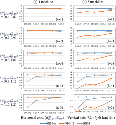
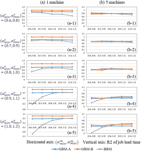
Figure 4. Generalization ability analysis of each model for System B.

Figure 3a shows the result for System A with single machine. GBM-A and GBM-B shows stable high accuracy regardless of the value of $\left({\alpha }_{min}^m,{\alpha }_{max}^m\right)$ and $\left({\alpha }_{min}^v,{\alpha }_{max}^v\right)$. It is because the parameter calibration of GBM-A and GBM-B succussed to find the global optimal solution in single machine case. On the other hand, the accuracy of BBM decreases in the case that $\left({\alpha }_{min}^m,{\alpha }_{max}^m\right)$ and $\left({\alpha }_{min}^v,{\alpha }_{max}^v\right)$ are different. This is a common trend in ML and is thought to be caused by overfitting to the modeling dataset. However, in the cases that $\left({\alpha }_{min}^v,{\alpha }_{max}^v\right)$ is low, the change in accuracy by the difference of $\left({\alpha }_{min}^m,{\alpha }_{max}^m\right)$ is small as shown Figures 3 (a-1) and (a-2). This result indicates that BBM trained using the data with sparse job arrivals, i.e., $\left({\alpha }_{min}^m,{\alpha }_{max}^m\right)$ is high, achieve high accuracy under dense arrival conditions, i.e., $\left({\alpha }_{min}^m,{\alpha }_{max}^m\right)$ is low. On the other hand, BBM trained using the data with dense arrival conditions shows low accuracy under sparse arrival conditions as shown in Figure 3 (a-5). This result indicates that BBM trained by data with sparse job arrival shows high generalization ability, but elucidating the cause of this result is a future issue.

Figure 3b shows the result for System A with five machines. In this case, the accuracy of GBM-B decreases because the parameter calibration by PSO fell into a local optimal solution. Since PSO is a heuristic optimization method, it is difficult to identify solid trends from these results, but the accuracy tends to increase as modeling dataset with sparse job arrivals. It is supposed that the difficulty in parameter calibration due to the model complexity becomes relatively low because the job queue in GBM may sometimes be empty under sparse arrival conditions.

Next, Figure 4a shows the result for System B with one machine. GBM-B and BBM shows a similar trend compared to the case of System A. The accuracy of GBM-A is relatively low, but the accuracy does not decrease even if $\left({\alpha }_{min}^m,{\alpha }_{max}^m\right)$ differ from $\left({\alpha }_{min}^v,{\alpha }_{max}^v\right)$. This result indicates that GBM-A does not overfit to the modeling datasets because of the low expressiveness of GBM-A.

Figure 4b shows the result for System B with five machines. In this case, the accuracy of all models decreases due to the complexity of target system. BBM outperforms GBMs when $\left({\alpha }_{min}^m,{\alpha }_{max}^m\right)$ is same and/or closed to $\left({\alpha }_{min}^v,{\alpha }_{max}^v\right)$, otherwise the superiority/inferiority are reversed.

In this experiment, the generalization ability of modeling methods for the changes in job arrival frequency is investigated. On the other hand, there are other possible changes in production systems such as machine failure in practice. For the case of machine failure, GBM has the advantage of being able to change the number of machines in the model explicitly, but BBM used in this paper does not have the capability to reflect the information of machine failure to the model. The evaluation and improvement of the generalization ability for such changes are future issues.

Conclusion

We proposed a novel modeling approach for material flow simulation, designated as data-driven and multi-scale simulation modeling, which aims to optimize model configuration in terms of simulation accuracy by combining various modeling methods. For this study, we conducted computational experiments for a virtual production system with single process to investigate the characteristics of modeling methods. Thereby, we obtained the following insights: (1) When the activity configuration of target system is partially unknown and/or the complexity of system is high, BBM may outperform GBM. (2) Compared to GBM, BBM is more sensitive to the difference between modeling and validation dataset, especially when applied to sparse job arrival conditions. (3) BBM trained by sparse job arrival conditions tend to show better accuracy and generalizability. The superiority and inferiority of modeling methods depend on the complexity of both systems and models, the background knowledge about the system and the possible changes in the system. These results indicates that the proposed modeling approach which combines various modeling methods is useful to obtain accurate simulation models since the characteristics of systems and background knowledge are varied in practical cases.

As future work, the authors intend to investigate the causes of (2). Additionally, experiments will be conducted for more complicated systems such as multiple processes to develop methods that optimize model configurations to realize the proposed concept.

Disclosure Statement

No potential conflict of interest was reported by the author(s).

Data Availability Statement

The data that support the findings of this study are available from the corresponding author, S.N., upon reasonable request.

References

- Barlas, P., and C. Heavey. 2016. Automation of input data to discrete event simulation for manufacturing: A review. International Journal of Modeling Simulation and Scientific Computing 7 (1):1630001. doi:10.1142/S1793962316300016.
- Choi, H., S. Ohmori, and K. Yoshimoto. 2011. Improvement of particle swarm optimization: Proposal of R-best model and parameter adjustment with consideration to searching phase and state. 21st International Conference on Production Research, Stuttgart, Germany, 2079–16.
- Henkenjohann, M., R. Joppen, D. Kochling, S. Enzberg, A. Kuhn, and R. Dumitrescu. 2021. Identification and specification of standard modules in production for a material flow simulation. Procedia CIRP 99:21–26. doi:10.1016/j.procir.2021.03.004.
- Hoellthaler, G., M. Schreiber, K. Vernickel, J. Isa, J. Fischer, N. Weinert, R. Rosen, and S. Braunreuther. 2019. Reconfiguration of production systems using optimization and material flow simulation. Procedia CIRP 81:133–38. doi:10.1016/j.procir.2019.03.024.
- Karnok, D., and L. Monostori. 2011. Determination of routings and process time information from event logs. IFAC Proceedings Volumes 44 (1):14055–60. doi:10.3182/20110828-6-IT-1002.01448.
- Kirchhof, P. 2016. Automatically generation flow shop simulation models from SAP data. Proceedings of the 2016 Winter Simulation Conference, Arlington, Virginia, USA, 3588–89.
- Lechner, M., P. Mothwurf, L. Nohe, and R. Daub. 2023. Material flow simulation in Lithium-ion battery cell manufacturing as a planning tool for cost and energy optimization. 5th Conference on Production Systems and Logistics, Stellenbosch, South Africa, 212–21.
- Lingitz, L., V. Gallina, F. Ansari, D. Gyulai, A. Pfeiffer, W. Sihn, and L. Monostori. 2018. Lead time prediction using machine learning algorithms: A case study by a semiconductor manufacturer. Procedia CIRP 72:1051–56. doi:10.1016/j.procir.2018.03.148.
- May, M. C., C. Nestroy, L. Overbeck, and G. Lanza. 2024. Automated model generation framework for material flow simulations of production systems. International Journal of Production Research 62 (1–2):141–56. doi:10.1080/00207543.2023.2284833.
- Monostori, L. 2014. Cyber-physical production systems: Roots, expectations and R&D challenges. Procedia CIRP 17:9–13. doi:10.1016/j.procir.2014.03.115.
- Nagahara, S., T. Kaihara, N. Fujii, and D. Kokuryo. 2022. A proposal of data-driven and multi-scale modeling approach for material flow simulation. IFIP WG 5.7 International Conference APMS 2022, Gyeongju, Korea, 297–215.
- Nagahara, S., S. Serita, Y. Shiho, S. Zheng, H. Wang, T. Chida, and C. Gupta. 2020. Toward data-driven modeling of material flow simulation: Automatic parameter calibration of multiple agents from sparse production log. 16th IEEE International Conference on Automation Science and Engineering, 1096–101.
- Nagahara, S., T. A. Sprock, and M. M. Helu. 2019. Toward data-driven production simulation modeling: Dispatching rule identification by machine learning techniques. Procedia CIRP 81:222–27. doi:10.1016/j.procir.2019.03.039.
- Popovics, G., and L. Monostori. 2013. ISA standard simulation model generation supported by data stored in low level controllers. Procedia CIRP 12:432–37. doi:10.1016/j.procir.2013.09.074.
- Rosen, R., G. Wichert, G. Lo, and K. D. Bettenhausen. 2015. About the importance of autonomy and digital twins for the future of manufacturing. IFAC-Papersonline 48 (3):567–72. doi:10.1016/j.ifacol.2015.06.141.
- Steinbacher, L. M., T. Düe, M. Veigt, and M. Freitag. 2023. Automatic model generation for material flow simulations of third-party logistics. Journal of Intelligent Manufacturing. doi:10.1007/s10845-023-02257-3.