Knowing how effective an intervention, treatment, or manipulation is and increasing replication rates: accuracy in parameter estimation as a partial solution to the replication crisis

Abstract

Objective

Although basing conclusions on confidence intervals for effect size estimates is preferred over relying on null hypothesis significance testing alone, confidence intervals in psychology are typically very wide. One reason may be a lack of easily applicable methods for planning studies to achieve sufficiently tight confidence intervals. This paper presents tables and freely accessible tools to facilitate planning studies for the desired accuracy in parameter estimation for a common effect size (Cohen’s d). In addition, the importance of such accuracy is demonstrated using data from the Reproducibility Project: Psychology (RPP).

Results

It is shown that the sampling distribution of Cohen’s d is very wide unless sample sizes are considerably larger than what is common in psychology studies. This means that effect size estimates can vary substantially from sample to sample, even with perfect replications. The RPP replications’ confidence intervals for Cohen’s d have widths of around 1 standard deviation (95% confidence interval from 1.05 to 1.39). Therefore, point estimates obtained in replications are likely to vary substantially from the estimates from earlier studies.

Conclusion

The implication is that researchers in psychology -and funders- will have to get used to conducting considerably larger studies if they are to build a strong evidence base.

Keywords:

• planning for precision
• confidence intervals
• accuracy in parameter estimation
• study planning
• sample size planning

As Cohen learned and taught, “the primary product of a research inquiry is one or more measures of effect size, not p values,” and, “having found the sample effect size, you can attach a p value to it, but it is far more informative to provide a confidence interval” (1990, p. 1310). Cohen was not alone in this conviction: the case for effect sizes and confidence intervals has been made excellently and extensively (Cohen, 1988, 1992; Cumming & Finch, 2001; Gardner & Altman, 1986; Thompson, 2002), and resulted in the imperative to always report confidence intervals (American Psychological Association, 2008, 2009). For example, the American Psychological Association “stresses that […] reporting elements such as effect sizes, confidence intervals, and extensive description are needed to convey the most complete meaning of the results” (2009, p. 33).

Despite this apparent consensus that psychological science would benefit from consistently computing effect size measures and their corresponding confidence intervals (note that confidence intervals comes with problems of their own, which we discuss in the discussion), few tools have been provided to facilitate planning studies for a desired confidence interval width. Power tables (Cohen, 1988, 1992) and software (Champely, 2016; Faul et al., 2007) for determining the required sample size when conducting null hypothesis significance tests (NHSTs) are quite common and well-known. However, if a researcher desires to obtain an association strength estimate (or, ‘effect size’ estimate¹) with a given accuracy in an experimental setting (i.e. a 95% confidence interval with a maximum width of .2 for a Cohen’s d_s² value that is estimated to be .4 in the population), then very few tools exist that are accessible to psychological researchers with a modest background in statistics. Maxwell, Kelley and Rausch do provide a visualisation of sample size requirements for confidence intervals (2008), but no tables or tools. The very insightful Effect Size Confidence Intervals (ESCI) spreadsheet accompanying Cumming (2014) and Cumming and Calin-Jageman (2016) does provide a dynamic interface allowing sample size computations, and is very helpful in understanding the dynamics at play as well. Other work is based on the sampling distribution of correlation coefficients, such as the script and tables provides by Moinester and Gottfried (Moinester & Gottfried, 2014; based on Bonett & Wright, 2000). Schönbrodt and Perugini introduced the Corridor of Stability to denote correlation estimates that are not only close to the true correlation (i.e. the population value), but which also remain close as data collection progresses (Lakens & Evers, 2014; Schönbrodt & Perugini, 2013).

These latter correlation-based approaches, while similar in their main message, rely on the (sometimes simulated) sampling distribution of Pearson’s r instead of that of Cohen’s d_s.³ This is problematic when planning experiments for two reasons. First, a relatively minor problem is that conversion between r and d is not a straightforward affair: for example, r = .3 converts to d_s = .63 instead of d_s = 0.5, and r = .5 converts to d_s = 1.15 instead of d_s = 0.8 (Cohen, 1988; McGrath & Meyer, 2006).⁴ This means that estimates for required sample sizes for experiments, derived from, for example, moderate (r = .3) or strong (r = .5) correlations, will underestimate the required sample sizes for moderate (d_s = 0.5) or large (d_s = 0.8) Cohen’s d_s values. More generally speaking: using correlation-based approaches may result in underestimates of the required sample sizes if the researcher is unaware of this and does not pay close attention.

Second, a major problem is that as we shall see further on, whereas the sampling distribution of the correlation coefficient becomes more narrow as the population correlation (i.e. the true effect size) approaches −1 or 1, this does not happen with the sampling distribution for Cohen’s d_s. In fact, the opposite happens: the sampling distribution of Cohen’s d_s becomes slightly wider as the difference between two means in the population increases. Individual values of d and r can be converted between the two metrics, but entire sampling distributions cannot. The 95% confidence interval for r = .5 is tighter than the 95% confidence interval for r = 0 (with equal sample sizes), but the 95% confidence interval for d_s = .8 is wider than the 95% confidence interval for d_s = 0.

Thus, currently, when planning an experiment to study whether an intervention, treatment, behaviour change principle (BCP, see Crutzen & Peters, 2018; such as Intervention Mapping’s behavior change methods, Kok et al., 2016, or a behavior change technique, BCT; Abraham & Michie, 2008) is effective (and therefore, how effective it is), researchers have limited access to free and easily accessible tools to compute the required sample size. This paucity of tools and the associated neglect to plan for accurate estimation of effects may in part explain why confidence intervals in psychological research are very wide (Brand & Bradley, 2016). In this paper, we provide both power tables and an easy to use tool to facilitate planning of studies that aim to draw conclusions about how effective a manipulation or treatment is with confidence intervals of a priori determined width.

Why confidence intervals are crucial in intervention evaluations

First, we will briefly summarize why confidence intervals are so valuable (albeit they still have their own interpretational problems; see the discussion). All point estimates computed from sample data, such as estimates of Cohen’s d_s or Pearson’s r, vary from sample to sample. Therefore, they are by themselves not informative when the goal is to learn about the population instead of about one random sample. A point estimate’s interpretation requires knowledge about how much it can be expected to vary from sample to sample, in other words, knowledge about its sampling distribution. A Cohen’s d_s of 0.5 might mean that in the population, two means differ by half a standard deviation, but if the corresponding sampling distribution is sufficiently wide, population values of 0.1 or 0.9 might also be plausible on the basis of that same dataset. Information about the variance of a statistic’s sampling distribution is most commonly conveyed using confidence intervals.

A confidence interval is an interval that will contain the population value of the corresponding statistic in a given percentage of the samples. For example, if in a sample of 100 participants a Cohen’s d_s value of 0.5 is found, the corresponding 95% confidence interval is [.10; .90] (see below for an explanation of this computation). This 95% confidence interval will contain the population value of Cohen’s d_s in 95% of the samples if the same study would be repeated infinitely.⁵ This interval is useful in that it allows inferring that, for example, a population value of −2 seems unlikely, and more generally, that any substantial harmful effects of this treatment seem unlikely. Computing an interval with a higher confidence level, such as 99% or 99.99%, makes it possible to make statements about the population with almost complete accuracy and certainty: only one in every 10 000 samples will not contain the population value in the 99.99% confidence interval.

In other words, confidence intervals around effect size measures are valuable instruments when the goal is to establish how strongly two variables are associated in the population, for example when establishing the effectiveness of a treatment, intervention, or the effect of a behaviour change technique or other experimental manipulation. Tight confidence intervals enable more confident statements about association strength (e.g., difference between conditions in an experiment), and therefore, researchers will usually want their confidence intervals to be as tight as possible. A common example is when researchers want to establish the likely population effect size in order to properly power a main study. In such a situation, researchers may conduct a pilot study to establish that effect size, and then power their main study accordingly, which makes acquiring an accurate effect size estimate a central concern.

For example, take the scenario above. Let us assume that a researcher correctly estimates a population value of d_pop = 0.5, and that the researcher then conducts a pilot study and coincidently happens to obtain a sample value of exactly d_s = 0.5. If the researcher obtains this value using two groups of 64 participants each, the corresponding confidence interval is [0.15; 0.85]. This means that on the basis of that one dataset, population values for Cohen’s d_pop of 0.15 and 0.85 (the lower and upper bounds of the confidence interval) are both equally likely. The high likelihood that the population value of Cohen’s d_pop is considerably lower than 0.5, the obtained point estimate, would make it unwise to power for that value of Cohen’s d. Instead, it would make sense to power for, for example, the lower bound of the confidence interval. In this case, if the researcher would want to use null hypothesis significance testing (NHST) for their main study, this would mean that the researcher would have to power their main study on Cohen’s d = .15. This would mean that the researcher would require 2312 participants to obtain a power of 95%, and 1398 participants to obtain a power of 80%. If the researcher had obtained a tighter confidence interval, this lower bound would have had a higher value, reflecting the higher certainty as to the population value of Cohen’s d_pop. One could argue that if the researcher had already obtained such an accurate estimation of the association (i.e., with a tight confidence interval), there would no longer be a need for another study that utilised NHST. This is a sensible argument, underlining the importance of basing required sample size estimates on desired confidence interval widths (Kraemer et al., 2006).

Tight confidence intervals are also valuable in other settings. For example, when conducting null hypothesis significance testing and rejecting a null hypothesis, the researcher concludes that it is likely that the two variables are associated in the population. However, without knowing how strongly the variables are associated, their association might have no practical or clinical significance. In addition, without some measure of association strength, the Numbers Needed to Treat (NNT; for an application to behavior change, see Gruijters & Peters, 2017) and cost effectiveness cannot be established. The researcher therefore commonly proceeds to compute a measure of association strength such as an effect size measure, but since the obtained point estimate changes value from sample to sample, it cannot inform the researchers of the likely association strength in the population. To conclude anything about the population, confidence intervals are normally computed, and given this intention to learn how strongly variables are associated in a population, researchers usually want these to be sufficiently tight.

When evaluating intervention effectiveness, it is clear that determining effect size is necessary for computing the NNT or cost effectiveness, and this also applies to the study of effectiveness of BCPs. However, in more fundamental (or basic) research, variables’ operationalisations sometimes have no meaningful scales, rendering effect sizes of secondary importance. In such studies, if no meaningful effect size estimate can be computed, the value of tight confidence intervals around the available effect size measures may be less clear at first glance. However, as will become clear, to yield results that are likely to replicate, such studies, too, require tight confidence intervals (or more accurately, narrow sampling distributions).

Thus, when planning a study, it can often be unwise if researchers limit themselves to computation of the sample size required to reject the null hypothesis in a given proportion of samples and given a specified expected association strength in the population (i.e. NHST-based power analysis). To be able to make useful statements about the likely strength of the studied association, researchers should also plan for confidence intervals of a given width. Although this point has been made repeatedly (e.g. Cumming, 2014; Maxwell et al., 2008), the width of confidence intervals in current psychological research (Brand & Bradley, 2016) implies that it has not yet been widely implemented. The tool we will now present is designed to facilitate this implementation in a situation where two groups of participants are compared.

How to compute the required sample size

We implemented this tool in the open source package ufs (Peters, 2019) for the open source statistical package R (R Core Team, 2018), which is often used in conjunction with the graphical user interface provided by the open source software RStudio (RStudio Team, 2019).⁶ We also implemented it in the ufs module for the open source application jamovi (jamovi project, 2019). We will first introduce the R package. To install this package, the following command can be used in an R analysis script or entered in the R console:

install.packages("ufs", repos="https://cran.rstudio.com/");

This command only needs to be run once: the package will remain installed. After installing the package, the following command can be used to request sample sizes:

ufs::pwr.cohensdCI(.5, w=.1);

The command above requests the sample size required to obtain a confidence interval with a margin of error (‘half-width’, argument ‘w’) of 0.1, assuming Cohen’s d_pop has a value of 0.5 in the population (the first argument, which can optionally be named ‘d’), therefore specifying a desired confidence interval with a total width of 0.2, from 0.4 to 0.6. This function will return the required total sample size. If a user wishes to receive more extensive results, the argument ‘extensive = TRUE’ can be used to also return the requested and obtained lower and upper bounds of the confidence interval, and the desired confidence level can be specified using argument ‘conf.level’ (the default confidence level of 95% is used when nothing is specified):

ufs::pwr.cohensdCI(.5, w=.1, extensive = TRUE); ufs::pwr.cohensdCI(.5, w=.1, conf.level=.99);

Under the hood, this function uses an iterative procedure where sample size is increased from 4 in steps of 100, then 10, then 1, to find the smallest sample size that yields a confidence interval with the desired width (or rather, tightness). To find the confidence interval of Cohen’s d_s, an approximation of the quantile function of the distribution of Cohen’s d is used. This approximation is achieved by converting the Cohen’s d value to Student’s t value and then using the quantile function of Student’s t to obtain the relevant t values, which are then converted back to Cohen’s d (using “MBESS::conf.limits.nct” from the “MBESS” package; Kelley, 2018; also see Kelley & Pornprasertmanit, 2016). This function to compute the confidence interval for a given confidence level, value of Cohen’s d_s and sample size is also available in the ufs package:

ufs::cohensdCI(.5, 128, .95);

The first argument specifies the point estimate of Cohen’s d_s, the second argument the sample size, and the third argument the desired confidence level (these can also be named using respectively ‘d’, ‘n’, and ‘conf.level’, the last of which has a default value of .95 and therefore can be omitted). This function returns the confidence interval.

The ufs jamovi module is an interface to these same R functions. The module can be installed from the jamovi library, and will add a ufs menu. This menu contains the analyses “Sample Size for Accuracy: Cohen’s d” (an interface to ufs::pwr.cohensdCI()) and “Effect Size Confidence Interval: Cohen’s d” (and interface to ufs::cohensdCI()). Selecting one of these analyses will open a dialog where the argument can be specified, after which the required sample size or resulting confidence interval is computed.

We have used the functions from the ufs R package to produce Table 1 (required sample sizes for 95% confidence intervals) and Table 2 (required sample sizes for 99% confidence intervals). Both tables show the required sample size for desired total confidence interval widths varying from a tenth of a standard deviation to an entire standard deviation for population values of Cohen’s d_pop of 0.2, 0.5, and 0.8 (the tentative qualitative labels denoting small, moderate, and strong associations). Two important implications follow from these tables.

Table 1. The required sample sizes for obtaining Cohen’s d_s 95% confidence intervals of the desired width.

	Desired confidence interval margin of error (‘half-width’)
d	0.05	0.1	0.15	0.2	0.25	0.3	0.35	0.4	0.45	0.5
0.2	6178	1545	687	387	248	172	127	97	77	62
0.5	6339	1585	705	397	254	177	130	100	79	64
0.8	6639	1660	738	416	266	185	136	104	83	67

Table 2. The required sample sizes for obtaining Cohen’s d_s 99% confidence intervals of the desired width.

	Desired confidence interval half-width
d	0.05	0.1	0.15	0.2	0.25	0.3	0.35	0.4	0.45	0.5
0.2	10669	2668	1186	667	427	297	218	167	132	107
0.5	10948	2737	1217	685	438	305	224	172	136	110
0.8	11466	2867	1275	717	459	319	235	180	142	115

First, it is important to realise that because, unlike Pearson’s r values, Cohen’s d and Student’s t values are not bounded, for Cohen’s d confidence intervals, the association strength does not matter much for the required sample size. Higher expected population values of Cohen’s d require slightly larger samples. This is opposite to the dynamics of correlation coefficient estimation, where for stronger associations, smaller samples suffice (Moinester & Gottfried, 2014). The difference is also much smaller than when estimating correlation coefficients: when estimating Cohen’s d values, differences in the expected population value have much less effect on the required sample size.

Second, the required sample sizes for somewhat precise estimation of effect sizes are considerably larger than those required to reject the null hypothesis assuming a given effect size: for comparison, the required sample sizes for detecting small, moderate, and strong associations with 80%, 90%, and 95% power are shown in Table 3. Although 128 participants suffice to detect a moderate effect with 80% power, the corresponding 95% confidence interval for d_s would run from 0.15 to 0.85; a total width of over half a standard deviation. In other words, on the basis of this dataset, it is not possible to say whether the effect would be trivial or large. And this is the situation when the point estimate represents a moderate effect: if instead a small effect is found, even with 128 participants, the 95% confidence interval for d_s runs from −0.15 to 0.55, so it would not be possible to say whether the effect is absent or of moderate strength in the population. To help get a firmer grasp of these dynamics, it can be useful to visualise the sampling distribution of Cohen’s d_s. To do this, the argument ‘plot = TRUE’ can be used when calling the ufs::cohensdCI() function:

Table 3. The required sample sizes for obtaining 80%, 90%, and 95% power.

	Desired power
d	80%	90%	95%
0.2	788	1054	1302
0.5	128	172	210
0.8	52	68	84

ufs::cohensdCI(d=.5, n = 128, plot = TRUE);

This function shows the sampling distribution of Cohen’s d for a given sample size, assuming that the specified value of Cohen’s d is the population value, and with the confidence interval shown. This sampling distribution is the distribution from which one value of Cohen’s d_s is randomly chosen when a study is conducted with the specified sample size, assuming that the association (or effect) in the population has the magnitude of the specified value of Cohen’s d_pop. Visualising this is useful when planning studies or interpreting results, as it helps to get a feel for the variation that can be expected in the obtained effect sizes. In this case, Figure 1 clearly illustrates the unpredictability of the obtained effect size estimate when a study is conducted with 128 participants in a situation where the population effect is Cohen’s d_pop = 0.5.

Figure 1. The sampling distribution of Cohen’s d for a population effect size of d_pop = 0.5 and a total sample size of 128 participants. Any Cohen’s d_s point estimate that is obtained in a study of 128 participants is drawn at random from this distribution, assuming that in the population, Cohen’s d_pop is indeed 0.5. The 95% confidence interval that a researcher would compute based on a sample estimate of d_s = 0.5 is shown in blue [.15;.85].

A sampling distribution-based perspective on the replication crisis

These wide sampling distributions mean that even when researchers power their studies quite highly for a given effect size for the purpose of null hypothesis significance testing, the obtained effect size estimates will still vary erratically from study to study. When studies are powered less strongly, and unfortunately most studies in psychology remain embarrassingly underpowered for all but the largest effect sizes (Bakker et al., 2012), observed effect sizes can vary even more. From this point of view, the somewhat depressing results of large-scale replication studies (e.g. Open Science Collaboration, 2015) seem to make sense. Most replicated studies (the original studies, that is) were extremely underpowered, even from an NHST point of view. This means that regardless of whether those original studies were correct regarding whether the hypothesized associations exist, the obtained effect sizes were pretty much random. To explore this, we selected all original studies with two-cell designs included in the Reproducibility Project: Psychology (Open Science Collaboration, 2015), available at https://osf.io/fgjvw. We extracted the sample sizes and effect size estimates from these studies and used these to construct the 95% confidence intervals.⁷ We repeated this using the sample sizes and effect sizes found in each study’s replication (valid statistics were extracted for 70 effect size estimates). Both sets of confidence intervals are shown in diamond plots (Peters, 2017) in Figure 2. From both sets of confidence intervals, we extracted the widths, and these are shown in Figure 3.

Figure 2. Confidence intervals for the original studies and replications in the Reproducibility Project: Psychology. Note the scale of the x axes.

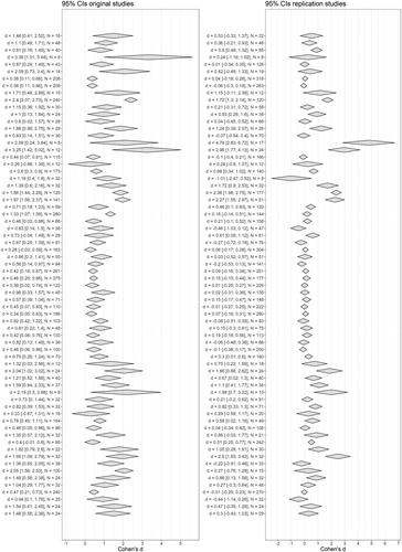
Figure 3. Confidence interval widths for the original studies and replications in the Reproducibility Project: Psychology.

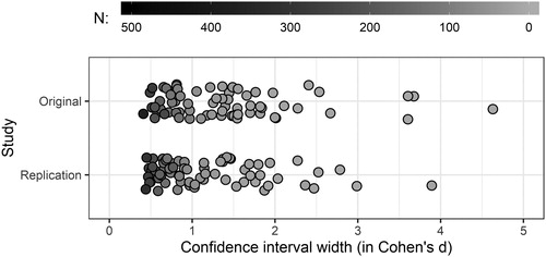
These figures confirm the expectations formulated above. The original studies did not allow accurate effect size estimates: in almost all cases, the effect size estimates’ sampling distributions were very wide. Even the replications do not allow accurate effect size estimates, again with confidence interval widths around 1 (the 95% confidence interval for the widths runs from 1.05 to 1.39 with a median width of 1.00). This means that the effect size estimates of these replications, too, were drawn from very wide sampling distributions. Therefore, replicating these replications with similar power (or more accurately, similar sample sizes) can yield very different effect size estimates. Note that although we used data from the Reproducibility Project: Psychology as an example, these wide sampling distributions can help explain results of other replication projects (e.g. Hagger et al., 2016) as well.

For determining how strongly two variables are associated, sample size estimates from power analyses based on null hypothesis significance testing are simply not good enough. This same logic holds for original research, of course. If researchers want their study to have a high likelihood of being replicable, the effect size they find should be drawn from a sufficiently narrow sampling distribution, or, in other words, the confidence intervals for their effect size estimates should be sufficiently tight. Tables 1 and 2 can help researchers to determine the sample size required for simple designs. For more complicated designs, where multivariate associations are estimated and sampling distributions are therefore conditional upon covariance between variables, each study may require a dedicated simulation to determine the required sample size. Researchers that do not have access to such simulations can at least use Tables 1 and 3 to get some sense of the order of magnitude of sample sizes one should consider.

Discussion

To determine whether an intervention is effective is to determine how effective an intervention is. After all, the knowledge that an effect is unlikely to be zero in a population has little value if that non-zero value might still represent a trivial effect. Determining whether an intervention is worthwhile requires establishing cost effectiveness, and such calculations will require accurate effect size estimates. Similarly, when studying behaviour change principles (BCPs, e.g., BCTs or Intervention Mapping’s methods for behaviour change), the goal is to establish how effective a given method can be for changing a given determinant (Kok et al., 2016; Peters et al., 2015). This information is required during intervention development to decide which behaviour change methods to select for targeting the relevant determinants (Kok, 2014). Therefore, health psychologists who evaluate intervention effectiveness or conduct experiments to examine the effectiveness of behaviour change principles may find Tables 1 and 2, as well as function ufs::pwr.cohensdCI(), useful. When using these tables and function to plan studies, the resulting body of evidence will be more likely to replicate. This will have as added advantage that such studies will do well when computing indices such as the replicability index, because the median power against all but the smallest effect sizes will be very high (Schimmack, 2016). Note, though, that replication depends on many other factors than sample size alone (Amrhein et al., 2019).

Shifting attention from null hypothesis significance tests to the accuracy of parameter estimates comes with a more acute awareness of the fact that any effect size estimate (in fact, anything computed from sample data) is randomly drawn from the corresponding sampling distribution. In every replication these estimates will take on different values, and the width of the sampling distribution determines how far these values can lie apart. Therefore, learning how effective an intervention is (therefore, whether it is effective), or learning how effective a BCP is (therefore, whether it is effective), or more generally, learning whether (therefore, how strongly) two variables are associated, requires narrow sampling distributions of the effect size estimate. Achieving sufficiently narrow sampling distributions, and therefore, tight confidence intervals and accurate parameter estimates, requires much larger sample sizes than are commonly seen in the literature. When surveying the literature, it would be easy to get the impression that experiments to assess the effectiveness of BCPs such as goal setting, implementation intentions, or fear appeals would require only a few dozen, or perhaps a few hundred participants. As the examples in this paper show, this is not true. Whereas for correlation coefficients, strong population effects mean that smaller samples suffice to achieve accurate estimates (Bonett & Wright, 2000; Moinester & Gottfried, 2014), for Cohen’s d_s (i.e., the effect size measure used for comparing two groups) the sampling distribution even becomes slightly wider as the population effect increases.

This shift from NHST to sampling distribution-based thinking (and the accompanying acute awareness of the instability of each sample point estimate) does not mean that estimation of association strengths should become the sole focus of health psychology research. It is important that parameter estimation is used in parallel with hypothesis testing. Not necessarily tests of the null hypothesis, nor significance tests using p values, let alone NHST (Cumming, 2014; Morey et al., 2014); but tests of theoretical hypotheses nonetheless (Morey et al., 2014). Sampling distribution-based thinking can facilitate formulating conditions for theory confirmation or refutation. For example, one can establish in advance which values should lie in the confidence interval or which should lie outside it, by committing oneself to considering a theory refuted by a dataset if a 99% confidence interval with a half-width of d = .1 includes values of .1 or lower. Such a scenario might be reasonable when testing the theoretical hypothesis that, for example, making coping plans has an effect on binge drinking. Note that setting these decision criteria (which confidence level to use, and how tight one wants the confidence interval to be) are inevitably subjective to a degree. The practice of full disclosure enables other researchers to apply different criteria to the same dataset (Peters et al., 2012).

Note that the results of equivalence tests, another approach to refuting theory (Lakens, 2017), can also vary wildly with small sample sizes. When using the Two One-Sided Tests (TOST) procedure, at an alpha of .05, one only requires 69 participants to have 80% power to reject associations stronger (or effects larger) than d = 0.5 (Lakens, 2017, Table 1). However, with 69 participants, the sampling distribution of Cohen’s d from which the point estimate for Cohen’s d_s that is obtained in any given study is drawn is still very wide. If the population value of Cohen’s d_pop is 0, the 95% confidence interval runs from −0.47 to 0.47; if the population d = 0.6, from 0.12 to 1.08. Even in this last scenario, obtaining a low point estimate of Cohen’s d in any given study is still quite plausible because the low sample size means that the point estimate is drawn from a very wide sampling distribution. TOST lacks consistent replicability as much as NHST unless the study is very highly powered (e.g. a power of 99% to detect (NHST) or reject (TOST) a small effect of d = 0.2).

Limitations

In its current version, the sample size planning function does not yet account for the desired assurance level. Assurance is a parameter that allows one to take into account the variation in sample variance from study to study. Like the mean, variance is a random variable, drawn at random from its sampling distribution. This variance (or rather, its square root, the standard deviation) is used to compute the standard error of the mean’s sampling distribution. Therefore, a researcher could be lucky and happen to obtain a relatively low variance estimate (and a tight confidence interval), or unlucky and obtain a relatively high variance estimate (and a wide confidence interval). Specifying the desired assurance allows a researcher to estimate the sample size required to obtain a confidence interval of the specified with in a given proportion of the studies. ESCI does allow the user to specify the desired assurance level (Cumming, 2014; Cumming & Calin-Jageman, 2016). It can therefore be useful to use both tools in parallel; the presently introduced R functions can be used to efficiently and reproducibly obtain a range of estimates for different scenarios, and once one or several scenarios have been selected, the estimates can be finetuned using ESCI. Note that taking the standard deviations’ sampling distribution into account by also parametrizing assurance leads to even higher sample size estimates. Therefore, the main message of the current paper, that NHST power analyses often substantially underestimate the sample sizes required to obtain replicable results, remains the same.

NHST, problems with confidence intervals, and Bayesian statistics

One of the reasons that use of NHST is discouraged in many situations is the widespread misinterpretation of p values (Amrhein et al., 2019; Wasserstein & Lazar, 2016; also see this special issue: Wasserstein et al., 2019). For example, Greenland et al. (2016) list 18 common misinterpretations of p values. This problem, however, is not entirely solved (though perhaps alleviated a bit) by using confidence intervals: the same authors list five common misinterpretations of confidence intervals (also see Morey et al., 2016). The first of these is the false belief that “[t]he specific 95% confidence interval presented by a study has a 95% chance of containing the true effect size.” This interpretation of confidence intervals is simultaneously widespread, intuitive, and wrong; and worse, frequentist methods cannot provide any such estimates. Instead, they yield an interval that, if the same study were repeated infinitely, will contain the population value in a given proportion of those studies. It would be much more informative to have an interval that, with a given probability, contains the population value.

Bayesian methods can provide such an interval, which is called the credible interval. Researchers trained in Bayesian methods, therefore, are inclined to compute credible intervals instead of confidence intervals. Unfortunately, many researchers are unfamiliar with Bayesian statistics (despite the increasing popularity of user friendly and freely available tools such as JASP; JASP Team, 2018). Fortunately, however, in situations where no informative prior is available, Bayesian methods and frequentist procedures tend to result in similar intervals (Albers et al., 2018; for another interesting exercise in comparing different statistical approaches, see Dongen et al., 2019). Because researchers who evaluate behaviour change interventions usually evaluate newly developed, complex, interventions, informative priors will rarely be available. Therefore, in such situations, thinking of a 95% confidence interval as an interval that has a 95% probability to contain the population effect size is hardly problematic in a practical sense (despite remaining formally incorrect, of course). Furthermore, even if confidence intervals are poorly understood, the shift towards sampling-distribution based thinking (i.e. a more acute awareness that all point estimates ‘dance around’ and as such, are often noninformative) that accompanies habitual use of confidence intervals remains valuable – also as a partial solution to the replication crisis.

Besides credible intervals, other approaches exist that can aid in sample size computations for accurate estimation. For example, the closeness procedure recommended by Trafimow et al. (2018) lets researchers compute the sample size required to obtain an estimate that, with a given confidence level, deviates no more than a given desired closeness from the population value. This approach is based on separate estimation of the means, as opposed to estimation of the difference between means. The variance of the sampling distribution of the difference (i.e. Cohen’s d) is larger than that of the sampling distribution of each mean, so which approach fits better depends on the researcher’s scenario (for details, see Trafimow, 2018). Note that when precise and replicable estimates are required, the methods yield similarly high sample size estimates (see Table 1 in Trafimow, 2018).

A related consideration is that, as Trafimow et al. (2018) argue, conclusions are ideally never based on single studies. Yet health psychologists often do applied research, working with politicians, policymakers, and stakeholder organisations, who often prefer (and sometimes demand) answers based on single studies, as opposed to waiting years or decades. Similarly, if funders fund the development of a behaviour change intervention, they commonly fund one evaluation study, not several. Both unfortunate facts of life often necessitate designing studies that allows conclusions that are as accurate as possible based on that single study.

Conclusion and implications

Concluding, we come to the somewhat depressing conclusion that the apparent norm in terms of sample sizes required for experimental research is a gross underestimation if the goal is to achieve replicable results. Replicable results require tight confidence intervals, because tight confidence intervals mean that the sampling distribution of the effect size is narrow, which means that in replications, effect size estimates of similar magnitude will be obtained. Conversely, if confidence intervals are wide, this means the sampling distribution of the effect size is wide, which means replications can obtain very different effect size point estimates. In such scenarios, significant results can easily disappear in a replication, and appear again in a third study. This has two implications.

First, funders should become aware of these dynamics, and cease funding small-scale studies. Conducting a psychological study will require more resources than funders (and researchers) are used to. On the other hand, there is no reason why conducting psychological studies should for some reason intrinsically be so much cheaper or quicker than in other fields. Creating the conditions necessary for studying the subject matter of a field has costs. In some fields, researchers require clean rooms (e.g. Peters & Tichem, 2016) or magnetic resonance imaging equipment (and also many participants; Szucs & Ioannidis, 2017). In psychology, the sampling and measurement error we have to deal with mean that to obtain sufficiently narrow sampling distributions for the associations we study, we require many measurements. Of course, ‘many measurements’ need not necessarily mean ‘many participants’, and in fact, intensive longitudinal methods are likely even a better solution when testing theories that make predictions about processes that occur within, rather than between, persons (see Inauen et al., 2016 for an excellent example; and see Naughton & Johnston, 2014 for an accessible introduction and tutorial of n-of-1 designs ). Regardless of whether measurements within or between participants are increased, funders will have to get used to considerably higher costs in terms of the time and funds required for one study.

Second, authors, reviewers, editors, and publishers and universities issuing press releases should be very tentative when drawing conclusions based on wide confidence intervals. Odds are, these conclusions will fail to replicate. Also, ethical review committees and institutional review boards should take this into account, to make sure that the scarce (often public) resources that are invested in research are not wasted on studies with sample sizes so low that the results are unlikely to replicate. In fact, for authors, reviewers, editors and publishers, these considerations are not only methodological, but ethical as well (Crutzen & Peters, 2017). Universities and publishers have a responsibility to critically assess their press releases, and there exists a point where an overenthusiastic press release becomes spreading of misinformation through neglect to properly scrutinize. It would be useful to start formulating rules of thumb as to how many datapoints are required before it is possible to have enough confidence in study outcomes to warrant a press release. Based on the present paper, one could, for example, argue that it is perhaps not justifiable to publish a press release about samples with only a hundred datapoints (especially if the study was an experiment; Peters & Gruijters, 2017).

On the bright side, once one has resigned to this unpleasant truth, a brilliant future may rise from the ashes. When using sufficiently large samples, very accurate statements can be made with high confidence. For example, with 750 participants (375 in each group), a 95% confidence interval for d_s = 0.2 has a total width of .29, which allows once to draw conclusions with relatively certainty: a moderate effect is unlikely to attenuate to a weak effect in a replication. These large sample sizes come with a bonus: even the 99% confidence interval has a total width of only .38. In a study with 1500 participants (750 in each group), a 95% confidence interval has a width of only .2, and at that sample size, a 99% confidence interval still has a total width of only .27, about a third of a standard deviation. This means that only in one out of hundred studies, the population effect size will lie outside the confidence interval, which means that for any given study, the likelihood that the population effect size will be captured in the confidence interval is very large. Another advantage is that in experiments with such high sample sizes, randomization is very likely to succeed, whereas with a few hundred participants, randomization may still plausibly result in non-equivalent groups with respect to a relevant moderator (Peters & Gruijters, 2017). Perhaps this is why it was rumoured that Cohen’s “idea of the perfect study is one with 10.000 cases and no variables” (Cohen, 1990, p. 1305).

Combined with full disclosure of materials and data (Crutzen et al., 2012; Peters et al., 2012) and complete transparency regarding the research proceedings (Peters et al., 2017), conducting studies with sufficiently large sample sizes to enable accurate parameter estimation enables building a solid basis of empirical evidence. If this is combined with careful testing, development (Earp & Trafimow, 2015) and application (Peters & Crutzen, 2017) of theory, this can yield a theory- and evidence base that can then confidently be used in the development of behaviour change interventions, eventually contributing to improvements in health and well-being. Conducting studies with sufficiently large sample sizes is as close to a guarantee of replication one is likely to come. This is an important message to funders as well: if the goal is to build a strong, replicable evidence base in psychology, it is necessary to fund studies with sample sizes that are considerably larger than what was funded in the past. However, although the price is high (literally), the promised rewards are plentiful.

Acknowledgements

We would like to thank Robert Calin-Jageman and Geoff Cumming for constructive corrections on the preprint of this paper, Guy Prochilo for pointing out an inconsistency in the algorithms and constructive comments, and the editor Rob Ruiter and reviewers Rink Hoekstra and David Trafimow for constructive comments during the peer review process.

Disclosure statement

No potential conflict of interest was reported by the author(s).

Notes

1 Statistically, all effects are simply associations: whether an association involves variables that are manipulated or only measured is theoretically crucial but statistically irrelevant.

2 Following Lakens (2013), we use the s subscript to unequivocally refer to the between-samples Cohen’s d; note that Goulet-Pelletier and Cousineau (2018) use d_p for this same form of Cohen’s d.

3 Note that the exact distribution of Pearson’s r is available in the R package SuppDists (Wheeler, 2016).

4 A number of free and easy-to-use tools exist that can help get a handle on how different values of r and d convert to each other. One is the FromR2D2 spreadsheet by Daniel Lakens, hosted at the Open Science Framework at https://osf.io/ixgcd. In addition, a family of conversion functions is available in the R package userfriendlyscience, such as convert.r.to.d and convert.d.to.r.

5 Note that whether this single confidence interval of [.10; .90] is among that 95% is not known: knowing this would require knowing the population value, knowledge of which would make collecting a sample redundant in the first place.

6 The analysis script and produced files are all available at the Open Science Framework at https://osf.io/5ejd8.

7 For some of these studies, no effect size estimate was available. For these studies, we constructed the confidence interval around zero to obtain the narrowest possible (i.e. most optimistic) confidence intervals.

References

- Abraham, C., & Michie, S. (2008). A taxonomy of behavior change techniques used in interventions. Health Psychology, 27(3), 379–387. https://doi.org/10.1037/0278-6133.27.3.379
- Albers, C. J., Kiers, H. A. L., & Van Ravenzwaaij, D. (2018). Credible confidence: A pragmatic view on the frequentist vs Bayesian debate. Collabra: Psychology, 4, 1–8.
- American Psychological Association. (2008). Reporting standards for research in psychology. The American Psychologist, 63(9), 839–851. https://doi.org/10.1037/0003-066X.63.9.839
- American Psychological Association. (2009). Publication manual of the American psychological association (6th ed.). APA.
- Amrhein, V., Greenland, S., & McShane, B. (2019). Scientists rise up against statistical significance. Nature, 567(7748), 305–307. https://doi.org/10.1038/d41586-019-00857-9
- Amrhein, V., Trafimow, D., & Greenland, S. (2019). Inferential statistics as descriptive statistics: There is no replication crisis if we don’t expect replication. The American Statistician, 73(sup1), 262–270. https://doi.org/10.1080/00031305.2018.1543137
- Bakker, M., Dijk, A. V., & Wicherts, J. M. (2012). The rules of the game called psychological science. Perspectives on Psychological Science, 7(6), 543–554. https://doi.org/10.1177/1745691612459060
- Bonett, D. G., & Wright, T. a. (2000). Sample size requirements for estimating pearson, kendall and spearman correlations. Psychometrika, 65(1), 23–28. https://doi.org/10.1007/BF02294183
- Brand, A., & Bradley, M. T. (2016). The precision of effect size estimation from published psychological research: Surveying confidence intervals. Psychological Reports, 118(1), 154–170. https://doi.org/10.1177/0033294115625265
- Champely, S. (2016). pwr: Basic functions for power analysis.
- Cohen, J. (1988). Statistical power analysis for the behavioral sciences (2nd ed.). Lawrence Erlbaum Associates.
- Cohen, J. (1990). Things I have learned (so far). American Psychologist, 45(12), 1304–1312. https://doi.org/10.1037/0003-066X.45.12.1304
- Cohen, J. (1992). A power primer. Psychological Bulletin, 112(1), 155–159. https://doi.org/10.1037/0033-2909.112.1.155
- Crutzen, R., Peters, G.-J Y., & Abraham, C. (2012). What about trialists sharing other study materials? BMJ, 345(6), e8352–e8352. https://doi.org/10.1136/bmj.e8352
- Crutzen, R., & Peters, G.-J Y. (2017). Targeting next generations to change the common practice of underpowered research. Frontiers in Psychology, 8, 1184. https://doi.org/10.3389/fpsyg.2017.01184
- Crutzen, R., & Peters, G.-J Y. (2018). Evolutionary learning processes as the foundation for behaviour change. Health Psychology Review, 12(1), 43–57. https://doi.org/10.1080/17437199.2017.1362569
- Cumming, G. (2014). The new statistics: Why and how. Psychological Science, 25(1), 7–29. https://doi.org/10.1177/0956797613504966
- Cumming, G., & Calin-Jageman, R. (2016). Introduction to the new statistics: Estimation, open science, and beyond. Routledge.
- Cumming, G., & Finch, S. (2001). A primer on the understanding, use, and calculation of confidence intervals that are based on central and noncentral distributions. Educational and Psychological Measurement, 61(4), 532–574. https://doi.org/10.1177/0013164401614002
- Dongen, N. N. N., van Doorn, J. B., Gronau, Q. F., van Ravenzwaaij, D., Hoekstra, R., Haucke, M. N., Lakens, D., Hennig, C., Morey, R. D., Homer, S., Gelman, A., Sprenger, J., & Wagenmakers, E.-J. (2019). Multiple perspectives on inference for two simple statistical scenarios. The American Statistician, 73(sup1), 328–339. https://doi.org/10.1080/00031305.2019.1565553
- Earp, B. D., & Trafimow, D. (2015). Replication, falsification, and the crisis of confidence in social psychology. Frontiers in Psychology, 6(5), 621. https://doi.org/10.3389/fpsyg.2015.00621
- Faul, F., Erdfelder, E., Lang, A.-G., & Buchner, A. (2007). G*Power 3: A flexible statistical power analysis program for the social, behavioral, and biomedical sciences. Behavior Research Methods, 39(2), 175–191. https://doi.org/10.3758/BF03193146
- Gardner, M. J., & Altman, D. G. (1986). Statistics in medicine confidence intervals rather than P values: Estimation rather than hypothesis testing. BMJ, 292(6522), 746–750. https://doi.org/10.1136/bmj.292.6522.746
- Goulet-Pelletier, J.-C., & Cousineau, D. (2018). A review of effect sizes and their confidence intervals, Part {I}: The Cohen’s d family. The Quantitative Methods for Psychology, 14(4), 242–265. https://doi.org/10.20982/tqmp.14.4.p242
- Greenland, S., Senn, S. J., Rothman, K. J., Carlin, J. B., Poole, C., Goodman, S. N., & Altman, D. G. (2016). Statistical tests, P values, confidence intervals, and power: A guide to misinterpretations. European Journal of Epidemiology, 31(4), 337–350. https://doi.org/10.1007/s10654-016-0149-3
- Gruijters, S. L. K., & Peters, G.-J Y. (2017). Introducing the Numbers Needed for Change (NNC): A practical measure of effect size for intervention research.
- Hagger, M. S., Chatzisarantis, N. L. D., Alberts, H., Anggono, C. O., Birt, A., Brand, R., Brandt, M. J., Brewer, G., Bruyneel, S., Calvillo, D. P., Campbell, W. K., Cannon, P. R., Carlucci, M., Carruth, N.P., Cheung, T., Crowell, A., De Ridder, D. T. D., Dewitte, S., Elson, M., … Zwienenberg, M. (2016). A multi-lab pre-registered replication of the ego-depletion effect. Perspectives on Psychological Science, 25(4), 1227–1234. https://doi.org/10.1177/0956797614526415.Data
- Inauen, J., Shrout, P. E., Bolger, N., Stadler, G., & Scholz, U. (2016). Mind the gap? An intensive longitudinal study of between-person and within-person intention-behavior relations. Annals of Behavioral Medicine, 50(4), 516–522. https://doi.org/10.1007/s12160-016-9776-x
- JASP Team. (2018). JASP (Version 0.9) [Computer software]. https://jasp-stats.org/.
- Kelley, K. (2018). MBESS: The MBESS R Package. https://CRAN.R-project.org/package=MBESS.
- Kelley, K., & Pornprasertmanit, S. (2016). Confidence intervals for population reliability coefficients: Evaluation of methods, recommendations, and software for composite measures. Psychological Methods, 21(1), 69–92. https://doi.org/10.1037/a0040086
- Kok, G. (2014). A practical guide to effective behavior change: How to apply theory- and evidence-based behavior change methods in an intervention. European Health Psychologist, 16(5), 156–170.
- Kok, G., Gottlieb, N. H., Peters, G.-J Y., Mullen, P. D., Parcel, G. S., Ruiter, R. A. C., Fernández, M. E., Markham, C., & Bartholomew, L. K. (2016). A taxonomy of behaviour change methods: An intervention mapping approach. Health Psychology Review, 10(3), 297–312. https://doi.org/10.1080/17437199.2015.1077155
- Kraemer, H. C., Mintz, J., Noda, A., Tinklenberg, J., & Yesavage, J. A. (2006). Caution regarding the use of pilot studies to guide power calculations for study proposals. Archives of General Psychiatry, 63(5), 484–489. https://doi.org/10.1001/archpsyc.63.5.484
- Lakens, D. (2013). Calculating and reporting effect sizes to facilitate cumulative science: A practical primer for t-tests and ANOVAs. Frontiers in Psychology, 4(11), 1–12. https://doi.org/10.3389/fpsyg.2013.00863
- Lakens, D. (2017). Equivalence tests: A practical primer for t-tests, correlations, and meta-analyses. Social Psychological and Personality Science, 8(4), 355–362. https://doi.org/10.1177/1948550617697177
- Lakens, D., & Evers, E. R. K. (2014). Sailing from the seas of chaos into the corridor of stability: Practical recommendations to increase the informational value of studies. Perspectives on Psychological Science, 9(3), 278–292. https://doi.org/10.1177/1745691614528520
- Maxwell, S. E., Kelley, K., & Rausch, J. R. (2008). Sample size planning for statistical power and accuracy in parameter estimation. Annual Review of Psychology, 59(1), 537–563. https://doi.org/10.1146/annurev.psych.59.103006.093735
- McGrath, R. E., & Meyer, G. J. (2006). When effect sizes disagree: The case of r and d. Psychological Methods, 11(4), 386–401. https://doi.org/10.1037/1082-989X.11.4.386
- Moinester, M., & Gottfried, R. (2014). Sample size estimation for correlations with pre-specified confidence interval. The Quantitative Methods for Psychology, 10(2), 124–130. https://doi.org/10.20982/tqmp.10.2.p0124
- Morey, R. D., Hoekstra, R., Rouder, J. N., Lee, M. D., & Wagenmakers, E. J. (2016). The fallacy of placing confidence in confidence intervals. Psychonomic Bulletin & Review, 23(1), 103–123. https://doi.org/10.3758/s13423-015-0947-8
- Morey, R. D., Rouder, J. N., Verhagen, J., & Wagenmakers, E.-J. (2014). Why hypothesis tests are essential for psychological science: A comment on cumming. Psychological Science, 25(6), 1289–1290. https://doi.org/10.1177/0956797614525969
- Naughton, F., & Johnston, D. (2014). A starter kit for undertaking n-of-1 trials. The European Health Psychologist, 16(5), 196–205.
- Open Science Collaboration. (2015). Estimating the reproducibility of psychological science. Science, 349, 6251. https://doi.org/10.1126/science.aac4716
- Peters, G.-J Y. (2017). Diamond plots: A tutorial to introduce a visualisation tool that facilitates interpretation and comparison of multiple sample estimates while respecting their inaccuracy. Health Psychology Bulletin, doi:10.31234/osf.io/fzh6c
- Peters, G.-J Y. (2019). ufs: Quantitative analysis made accessible. https://ufs.opens.science.
- Peters, G.-J Y., Abraham, C. S., & Crutzen, R. (2012). Full disclosure: Doing behavioural science necessitates sharing. The European Health Psychologist, 14(4), 77–84.
- Peters, G.-J Y., & Crutzen, R. (2017). Pragmatic Nihilism: How a theory of nothing can help health psychology progress. Health Psychology Review, 11(2), 103–121. https://doi.org/10.1080/17437199.2017.1284015
- Peters, G.-J Y., de Bruin, M., & Crutzen, R. (2015). Everything should be as simple as possible, but no simpler: Towards a protocol for accumulating evidence regarding the active content of health behaviour change interventions. Health Psychology Review, 9(1), 1–14. https://doi.org/10.1080/17437199.2013.848409
- Peters, G.-J Y., & Gruijters, S. L. K. (2017). Why most experiments in psychology failed: Sample sizes required for randomization to generate equivalent groups as a partial solution to the replication crisis [Doctoral dissertation]. Maastricht University.
- Peters, G.-J Y., Kok, G., Crutzen, R., & Sanderman, R. (2017). Health Psychology Bulletin: Improving publication practices to accelerate scientific progress. Health Psychology Bulletin, 1(1), 1–6. https://doi.org/10.5334/hpb.2
- Peters, T.-J., & Tichem, M. (2016). Electrothermal actuators for SiO2 photonic MEMS. Micromachines, 7(11), 200. https://doi.org/10.3390/mi7110200
- R Core Team. (2018). R: A language and environment for statistical computing. https://www.R-project.org/.
- RStudio Team. (2019). RStudio: Integrated development environment for R. http://www.rstudio.com/.
- Schimmack, U. (2016). The replicability-index: Quantifying statistical research integrity. https://wordpress.com/post/replication-index.wordpress.com/920.
- Schönbrodt, F. D., & Perugini, M. (2013). At what sample size do correlations stabilize? Journal of Research in Personality, 47(5), 609–612. https://doi.org/10.1016/j.jrp.2013.05.009
- Szucs, D., & Ioannidis, J. P. (2017). Empirical assessment of published effect sizes and power in the recent cognitive neuroscience and psychology literature. PLOS Biology, 15(3), e2000797. https://doi.org/10.1371/journal.pbio.2000797
- Thompson, B. (2002). What future quantitative social science research could look like: Confidence intervals for effect sizes. Educational Researcher, 31(3), 25–32. https://doi.org/10.3102/0013189X031003025
- Trafimow, D. (2018). An a priori solution to the replication crisis. Philosophical Psychology, 31(8), 1188–1214. https://doi.org/10.1080/09515089.2018.1490707
- Trafimow, D., Amrhein, V., Areshenkoff, C. N., Barrera-Causil, C. J., Beh, E. J., Bilgiç, Y. K., Bono, R., Bradley, M. T., Briggs, W. M., Cepeda-Freyre, H. A., Chaigneau, S. E., Ciocca, D. R., Correa, J. C., Cousineau, D., de Boer, M. R., Dhar, S. S., Dolgov, I., Gómez-Benito, J., Grendar, M., … Marmolejo-Ramos, F. (2018). Manipulating the alpha level cannot cure significance testing. Frontiers in Psychology, 9, 699. https://doi.org/10.3389/fpsyg.2018.00699
- Wasserstein, R. L., & Lazar, N. A. (2016). The ASA’s statement on p-values: Context, process, and purpose. The American Statistician, 70(2), 129–133. https://doi.org/10.1080/00031305.2016.1154108
- Wasserstein, R. L., Schirm, A. L., & Lazar, N. A. (2019). Moving to a world beyond “p < 0.05”. The American Statistician, 73(sup1), 1–19. https://doi.org/10.1080/00031305.2019.1583913
- Wheeler, B. (2016). SuppDists: Supplementary distributions. R package version 1.1-9.4.