Towards an absolute scale for adhesion strength of ship hull microfouling

Abstract

In-water ships’ hull cleaning enables significant fuel savings through removal of marine fouling from surfaces. However, cleaning may also shorten the lifetime of hull coatings, with a subsequent increase in the colonization and growth rate of fouling organisms. Deleterious effects of cleaning would be minimized by matching cleaning forces to the adhesion strength of the early stages of fouling, or microfouling. Calibrated waterjets are routinely used to compare different coatings in terms of the adhesion strength of microfouling. However, an absolute scale is lacking for translating such results into cleaning forces, which are of interest for the design and operation of hull cleaning devices. This paper discusses how such forces can be determined using computational fluid dynamics. Semi-empirical formulae are derived for forces under immersed waterjets, where the normal and tangential components of wall forces are given as functions of different flow parameters. Nozzle translation speed is identified as a parameter for future research, as this may affect cleaning efficacy.

Keywords:

• Adhesion strength
• marine fouling
• ship hull fouling
• microfouling
• calibrated waterjet
• energy efficiency

Introduction

In-water cleaning reduces the amount of biofouling on ships’ hulls. Cleaning may also have the benefit of reactivating biocide release from antifouling coatings on a short time frame (Morrisey and Woods 2015). However, if cleaning events create damage, these may shorten the lifetime of the coatings, potentially resulting in a higher degree of biofouling (Malone 1980; Munk, Kane, and Yebra 2009). It is thus essential to gain knowledge on the forces required to remove early stages of fouling from ships’ hull coatings, commonly referred to as the adhesion strength of microfouling (Oliveira and Granhag 2016).

Biofouling on ships’ hulls and propellers is a burden from both the environmental and economic perspectives. It leads to increased hydrodynamic resistance and increased propulsion powering, resulting in fuel penalties and correspondingly increased emissions to the air from shipping (Schultz 2007). Also, the transport of aquatic organisms on ships’ hulls represents a biosecurity risk: the potential spread of non-native invasive species may impact both marine ecosystems and economic activities (Davidson et al. 2016).

Today, hull fouling is reduced using a combination of fouling-control coatings and in-water maintenance (Oliveira and Granhag 2016). Commercial fouling-control coatings are broadly grouped into two types: biocide-containing antifouling coatings (AF), and non-toxic foul-release coatings (FR), the latter exhibiting low surface adhesion properties (Yebra, Kiil, and Dam-Johansen 2004). Although each of these coatings is usually effective in avoiding fouling under specific conditions, today’s ships still require in-water cleaning to mechanically remove fouling from the hull. Such cleanings rely on either diver-operated or remotely operated cleaning devices (IMO 2011; Morrisey and Woods 2015).

When it comes to in-water hull cleaning, the aim is to remove fouling with minimal wear/damage to the hull coating system, thus maximizing the lifetime of the coating (Holm, Haslbeck, and Horinek 2003; Naval Sea Systems Command 2006). A hull grooming strategy has therefore been recommended, consisting of gentle and frequent cleanings (Tribou and Swain 2015; Tribou and Swain 2017). Hull grooming enables fuel savings and avoids increased emissions to the air from shipping (Hunsucker et al. 2018). Also, hull grooming targets the early stages of marine fouling, ie microfouling, which typically requires lower cleaning forces than more advanced stages of fouling, ie macrofouling (Oliveira and Granhag 2016).

The matching of cleaning forces to the adhesion strength of microfouling would likely result in better design and fine-tuning of operational parameters in hull cleaning devices, with both environmental and economic benefits. On the one hand, minimizing cleaning forces would reduce the amount of biocides released to the environment during cleaning events (Schiff, Diehl, and Valkirs 2004). On the other hand, extending the lifetime of the paint would enable economic savings for ship operators, by reducing painting costs in dry-dock maintenance, as well as voyage costs (Schultz et al. 2011; Hearin et al. 2015).

Two main techniques are reported in the literature for determining the adhesion strength of microfouling on ships’ hull coatings: a turbulent channel flow apparatus (Schultz et al. 2000) and a calibrated waterjet (Swain and Schultz 1996; Finlay et al. 2002; Hunsucker and Swain 2016). Other techniques have been used for studying adhesion, such as rotating discs (Ackerman et al. 1992) and atomic force microscopy (AFM; Callow et al. 2000). The latter techniques either produce force gradients, in the case of rotating disks, or focus on determining microscopic forces at the cell/adhesive level, in the case of AFM. As these techniques do not yield results required for directly matching in-water cleaning forces to adhesion strength (Oliveira and Granhag 2016), they will not be detailed here.

A turbulent channel flow apparatus relies on known tangential forces to evaluate the FR properties of coatings, using wall shear stress as a measure of adhesion strength of microfouling, in N m⁻² (or Pa). The tangential forces created in this test can then be directly compared to forces experienced by microfouling on a moving hull, ie for predicting detachment while the ship is underway (Schultz et al. 2003). Therefore, these tests produce valuable results for evaluating the efficacy of FR coatings under design conditions.

Calibrated waterjets achieve higher shear forces than a turbulent channel flow apparatus (Finlay et al. 2002). The principle is to obtain a controlled flow of water, issuing from a nozzle pointed vertically at the fouled sample, thus producing both normal and tangential forces on the sample (Swain and Schultz 1996). This type of flow resembles that observed in waterjet hull cleaning systems, which are currently used worldwide (Morrisey and Woods 2015). Thus, calibrated waterjets are suited for the purpose of determining cleaning forces required during in-water hull cleaning.

For calibrated waterjets, there is still no standard definition of adhesion strength. Some authors report adhesion strength in terms of impact pressure, loosely defined as the normal force divided by the ‘area over which the water exerted an effect’ (Swain and Schultz 1996; Finlay et al. 2002). Other authors report surface pressure, defined as the normal force divided by a given area over which the force measurement is performed (Hunsucker and Swain 2016). In addition, the maximum wall shear stress under a vertically impinging jet (Finlay et al. 2002) has also been estimated using a semi-empirical formula for vertically impinging immersed jets (Beltaos and Rajaratnam 1974). However, the latter formula was challenged, as reviewed below (see Review on round immersed impinging jets). Also, this formula was originally derived for immersed jets, which likely leads to underestimation of the forces experienced under the water-in-air jets used in previous studies on adhesion strength of microfouling (Swain and Schultz 1996; Finlay et al. 2002). Thus, due to the lack of a standard definition of adhesion strength and the ‘ephemeral nature’ of microfouling, results have so far been discussed only in terms of local comparison between different coating formulations or FR products (Swain and Schultz 1996; Hunsucker and Swain 2016).

The aim of the current investigation was to enable the matching of in-water hull cleaning forces to the adhesion strength of microfouling by providing a more accurate description of forces under impinging jets, using semi-empirical formulae for immersed calibrated waterjets. Specifically, the relation between tangential and normal components of surface forces was analysed using computational fluid dynamics (CFD).

In the following sub-section, a short review is given on previous work on round immersed jets, specifically focusing on wall surface forces. This is followed by a report of the present numerical simulations on the flow problem of an immersed calibrated waterjet, using a CFD approach. Finally, recommendations are given regarding the applicability of semi-empirical formulae, as well as considerations on translation speed, temperature and water quality.

Review on round immersed impinging jets

Round vertically impinging jets under immersed conditions, ie water-in-water jets or air-in-air jets, have been extensively studied in the past. These jets are of interest in many fields of engineering, from aerospace (Wu, Banyassady, and Piomelli 2016) to heating/cooling, metal cutting and industrial cleaning (Shademan et al. 2016), as well as in soil erosion testing (Hanson and Cook 2004).

The flow problem is generally defined as follows (Figure 1a): a viscous fluid (viscosity ν ≠ 0) issues at a given mean velocity u₀ from a nozzle exit, with inner diameter D, being vertically directed at an opposing wall at a stand-off distance H from the nozzle exit. A selection of publications on this specific flow problem is listed in Table 1. These are discussed below in terms of dimensionless stand-off distance H/D, Reynolds number Re based on nozzle diameter, technique used for determining wall shear stress, and nozzle type.

Figure 1. Geometry and boundary conditions: (a) schematic representation of a vertically impinging jet; (b) boundary conditions for axisymmetric cases simulated in the present study, where the symmetry axis coincides with the x axis. The drawings are not to scale.

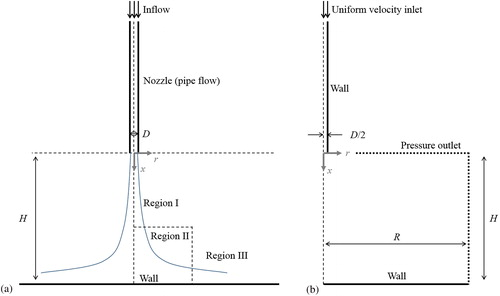
Table 1. Previous experimental and numerical studies on vertically impinging circular jets.

Reference	H/D	Re	Technique for wall shear stress	Nozzle type
Bradshaw & Love (1961)	18	1.5 × 10^5	Flat Preston tube (air)	Pipe
Poreh, Tsuei, and Cermak (1967)	8–24	1.11 × 10^6–5.00 × 10^6	Floating element (air)	Orifice
Kataoka & Mizushina (1974)	3.86–8.24	9.60 × 10^3–3.62 × 10^4	Electro-chemical (water)	Convergent
Beltaos & Rajaratnam (1974)	21.2–65.7	3.89 × 10^4–8.04 × 10^4	Preston tube (air)	Convergent
Giralt, Chia, and Trass (1977)	3.0–25.0	3 × 10^4–8 × 10^4	Not determined (air)	Convergent
Hanson, Robinson, and Temple (1990)	16.5	2.3 × 10^4–8.4 × 10^4	Hot-film sensor (water)	Convergent
Alekseenko & Markovich (1994)	2–8	4.16 × 10^4	Electrochemical (water)	Convergent
Phares, Smedley, and Flagan (2000)	3–20	3.7 × 10^3–1.15 × 10^4	Particle resuspension (air)	Short pipe
Shademan, Balachandar, and Barron (2013)	2–18.5	1 × 10^5	RANS	Uniform inlet
Ghaneeizad, Atkinson, and Bennett (2015)	24.7	2.3 × 10^4–3.4 × 10^4	PIV (water)	JET nozzle
Shademan et al. (2016)	20	2.8 × 10^4	LES, PIV (water)	Convergent

RANS, Reynolds-averaged Navier–Stokes; LES, large eddy simulation; PIV, particle image velocimetry; JET, jet erosion test.

In terms of stand-off distance, the present focus is on fully developed jets, ie H/D ≥ 8 (Phares, Smedley, and Flagan 2000). Calibrated waterjets used in adhesion testing are typically fully developed, where a value H/D $\approx$ 15.6 is commonly reported (eg Finlay et al. 2002; Hunsucker and Swain 2016). Fully developed jets are usually described in terms of three distinct regions, as represented in Figure 1a, which are characterized as follows (Beltaos and Rajaratnam 1974): Region I – free jet region, where the flow is identical to that of a free jet; Region II – the impingement region, where the flow is increasingly deflected from axial to radial direction in the presence of a wall; and Region III – wall jet region, where the flow is practically parallel to the wall.

In Table 1, the Reynolds number Re based on nozzle diameter ranges between ∼10³ and ∼10⁶, which frames the values used in calibrated waterjets for microfouling adhesion testing, typically around Re ∼10⁴ (Finlay et al. 2002). This means that the ratio between inertia and viscous forces (Reynolds number) is similar, and therefore previous work may be used for validation and calibration purposes.

Depending on the working fluid, usually air or water, different experimental techniques have been used in the past for determining the tangential component of wall surface forces, ie the wall shear stress (Table 1). For air-in-air jets, Preston tubes and particle resuspension techniques have been reported. For water-in-water jets, electrochemical methods, hot-film sensors and particle image velocimetry (PIV) have been reported. These methods differ in terms of accuracy, where electrochemical methods are generally considered the most accurate as discussed in Phares, Smedley, and Flagan (2000).

Nozzle geometry also varies between different studies: from simple round orifices on plates (eg Poreh, Tsuei, and Cermak 1967), to pipe-flow nozzles (eg Bradshaw and Love 1961) and convergent nozzles (eg Beltaos and Rajaratnam 1974). Other nozzles have also been reported, such as the jet erosion test (JET) nozzle, in the field of soil erosion (Hanson and Cook 2004; Ghaneeizad et al. 2015). Nozzle geometry is known to affect heat transfer near the impingement to a certain degree, through changing the turbulence intensity and velocity profile at the nozzle exit. Such differences are more significant for low stand-off distances (Jambunathan et al. 1992). Thus, nozzle geometry can have some scattering effect in the results obtained with different nozzle types (Xu and Antonia 2002).

For fully developed jets (H/D ≥ 8), dimensional analysis has been used to describe wall surface forces as a function of jet flow parameters, ie stand-off distance H, nozzle diameter D, fluid velocity at the nozzle u₀, and fluid properties (Beltaos and Rajaratnam 1974; Phares, Smedley, and Flagan 2000). Thus, Beltaos and Rajaratnam (1974) arrived at semi-empirical formulae for time-averaged wall surface forces, namely stagnation pressure $p_s$ and maximum wall shear stress ${\tau }_{w,\mathit{max}}:$ (1) $$p_s=25\frac{\rho {u_0}^2}{{\left(H/D\right)}^2}, \mathrm{at}\mathrm{ }r/H =\mathrm{ }0$$(1) (2) $${\tau }_{w,\mathit{max}}=0.16\frac{\rho {u_0}^2}{{\left(H/D\right)}^2}, \mathrm{at}\mathrm{ }r/H =\mathrm{ }0.14$$(2) where $\rho$ is the density of the fluid and r is the radial distance from the impingement. According to Equations 1(1) $$p_s=25\frac{\rho {u_0}^2}{{\left(H/D\right)}^2}, \mathrm{at}\mathrm{ }r/H =\mathrm{ }0$$(1) and 2(2) $${\tau }_{w,\mathit{max}}=0.16\frac{\rho {u_0}^2}{{\left(H/D\right)}^2}, \mathrm{at}\mathrm{ }r/H =\mathrm{ }0.14$$(2) , $p_s$ and ${\tau }_{w,\mathit{max}}$ are both proportional to the same combination of flow parameters, ie $\rho {u_0}^2/{\left(H/D\right)}^2,$ and it is then trivial to conclude that these two forces are linearly correlated, ie $p_s\approx 156\mathrm{ }{\tau }_{w,\mathit{max}}.$ However, Phares, Smedley, and Flagan (2000) identified flaws in the derivation of Equation 2(2) $${\tau }_{w,\mathit{max}}=0.16\frac{\rho {u_0}^2}{{\left(H/D\right)}^2}, \mathrm{at}\mathrm{ }r/H =\mathrm{ }0.14$$(2) by Beltaos and Rajaratnam (1974) and provided their own relation for maximum wall shear stress under fully developed jets (H/D ≥ 8), including the Reynolds number at the nozzle, Re: (3) $${\tau }_{w,m}=44.6\frac{\rho {u_0}^2{\mathit{Re}}^{-\frac{1}{2}}}{{\left(H/D\right)}^2}, \mathrm{at}\mathrm{ }r/H =\mathrm{ }0.09$$(3)

Phares, Smedley, and Flagan (2000) based this relation on laminar boundary layer theory, assuming that the strong favourable pressure gradient near the stagnation point would laminarize the boundary layer (Phares, Smedley, and Flagan 2000). However, it is arguable whether an exponent in the Reynolds number of −1/2 in Equation 3(3) $${\tau }_{w,m}=44.6\frac{\rho {u_0}^2{\mathit{Re}}^{-\frac{1}{2}}}{{\left(H/D\right)}^2}, \mathrm{at}\mathrm{ }r/H =\mathrm{ }0.09$$(3) can be used to generalize for all fully developed jets. This exponent of −1/2 is based on the assumption of laminar flow, while it seems likely that the maximum wall shear stress actually occurs under turbulent flow: for fully developed jets (H/D > 8), results from several authors fail to show any secondary peak in wall shear stress at radii larger than the location of maximum wall shear stress, ie r/H > 0.1 (Bradshaw and Love 1961; Beltaos and Rajaratnam 1974; Hanson, Robinson, and Temple 1990), and this seems to suggest that the transition from laminar to turbulent flow occurs upstream from the maximum wall shear stress. Such secondary peaks have only been observed for developing jets, with stand-off ratios H/D < 8 (Kataoka and Mizushina 1974; Alekseenko and Markovich 1994). Thus, the assumption of laminar flow at the maximum wall shear stress does not seem to hold for fully developed jets, and an exponent in the Reynolds number of −1/2 might not be appropriate.

In the current paper, a numerical approach is used to simulate immersed vertically impinging jets, using a CFD approach based on Shademan, Balachandar, and Barron (2013) with the aim of evaluating scaling parameters for wall surface forces under calibrated waterjets used in microfouling adhesion strength tests (Swain and Schultz 1996; Finlay et al. 2002). Specifically, an adequate exponent for the Reynolds number in Equation 3(3) $${\tau }_{w,m}=44.6\frac{\rho {u_0}^2{\mathit{Re}}^{-\frac{1}{2}}}{{\left(H/D\right)}^2}, \mathrm{at}\mathrm{ }r/H =\mathrm{ }0.09$$(3) is sought. The applicability of the semi-empirical formulae obtained is then discussed from the perspective of microfouling adhesion strength testing for matching in-water hull cleaning forces.

Materials and methods

In this section, a numerical approach is described to simulate vertically impinging immersed jets (water-in-water jets) using CFD.

Geometry and boundary conditions

Figure 1a gives a schematic representation of a vertically impinging jet. The x-axis is located at the jet’s centreline, and the origin of both x and radial distance r is located at the nozzle’s exit. In this study, axisymmetric cases were simulated, since the time-averaged flow of a round vertically impinging jet is axisymmetric, ie the mean velocity and pressure fields are expected to be the same at every radius. Thus, instead of computing the jet in three-dimensional coordinates, which would mean an unnecessary increase in computation cost, the flow is computed on an axisymmetric section along a radius, as represented in Figure 1b. This represents the case of a controlled experiment, where adhesion strength testing is performed with a single nozzle positioned accurately at a given distance from a flat sample surface.

Boundary conditions used in this study are identified in Figure 1b, where the axisymmetric numerical domain is represented. The nozzle corresponds to a straight pipe with diameter D and uniform velocity inlet. From the exit of the nozzle, the jet develops into a cylindrical chamber, bounded by a smooth no-slip wall opposite to the nozzle, at a stand-off distance H from the nozzle exit. The remaining boundaries are defined as pressure outlets, with zero relative pressure (atmospheric pressure). The total radial length of the numerical domain is denoted by R.

Simulated flow cases are defined in Table 2, where a stand-off ratio of H/D = 20 was kept throughout. The first case, with nozzle diameter D = 0.01 m, is used for validation against experimental and numerical results from Shademan et al. (2016). The four remaining cases, with nozzle diameter D = 1.6 mm, represent conditions specific to microfouling adhesion tests using calibrated waterjets (Swain and Schultz 1996; Finlay et al. 2002), with the sole difference that here the waterjets are immersed, rather than in air. These latter four cases are the basis for the present empirical study, aimed at finding scaling parameters for surface forces.

Table 2. Flow cases simulated in this study, where H/D = 20 is used throughout.

D [m]	Re	u0 [m s^−1]	Purpose
0.01	28,000	2.811	Validation (Shademan et al. 2016)
0.0016	7,000	4.4	Empirical study on scaling parameters (adhesion testing)
	18,000	11.3
	29,000	18.2
	40,000	25.1

In the empirical study, Reynolds number is based on nozzle diameter varied from 7,000 to 40,000 by varying the average speed at the nozzle u₀ in the range 4.4–25.1 m s⁻¹. In comparison, adhesion strength tests ran by Finlay et al. (2002) relied on speeds at the nozzle estimated roughly as ∼5–20 m s⁻¹, to test adhesion of spores of Ulva sp. on glass, which has low FR properties and should therefore give an upper limit to adhesion strength.

Numerical method

To simulate the above cases, continuity and momentum equations, or Reynolds averaged Navier–Stokes (RANS) equations, were solved in incompressible steady state using the commercial CFD code STAR-CCM+, version 11.02.010-R8 for Windows 64-bit (CD-adapco™, Melville, NY, USA): (4) $$\rho \frac{\partial {\overline{u}}_i}{\partial x_i}=0$$(4) (5) $$\frac{\partial }{\partial x_j}\left({\overline{u}}_i{\overline{u}}_j\right)=-\frac{1}{\rho }\frac{\partial \overline{p}}{\partial x_i}+\frac{\partial }{\partial x_j}\left[\nu \left(\frac{\partial {\overline{u}}_i}{\partial x_j}+\frac{\partial {\overline{u}}_j}{\partial x_i}\right)\right]+\frac{1}{\rho }\frac{\partial }{\partial x_j}\left(-\rho \mathrm{ }\overline{{u\mathrm{\prime }}_i^{\mathrm{ }}{u\mathrm{\prime }}_j^{\mathrm{ }}}\right)$$(5) where ${\overline{u}}_i$ is the time-averaged velocity component in the Cartesian direction i, and the product $-\rho \mathrm{ }\overline{{u\mathrm{\text{'}}}_i^{\mathrm{ }}{u\mathrm{\text{'}}}_j^{\mathrm{ }}}$ represents the Reynolds stresses obtained from turbulence modelling. In Equation 5(5) $$\frac{\partial }{\partial x_j}\left({\overline{u}}_i{\overline{u}}_j\right)=-\frac{1}{\rho }\frac{\partial \overline{p}}{\partial x_i}+\frac{\partial }{\partial x_j}\left[\nu \left(\frac{\partial {\overline{u}}_i}{\partial x_j}+\frac{\partial {\overline{u}}_j}{\partial x_i}\right)\right]+\frac{1}{\rho }\frac{\partial }{\partial x_j}\left(-\rho \mathrm{ }\overline{{u\mathrm{\prime }}_i^{\mathrm{ }}{u\mathrm{\prime }}_j^{\mathrm{ }}}\right)$$(5) , the gravity term is neglected (no buoyancy effects), and pressure $p$ corresponds to hydrodynamic pressure (Larsson and Raven 2010, p. 9). Constant properties were selected, corresponding to freshwater at a temperature of 20 °C: ρ = 998 kg m⁻³ and $\mu$ = 1.002 × 10⁻³Pa s⁻¹. The commercial CFD code discretizes Equations 4(4) $$\rho \frac{\partial {\overline{u}}_i}{\partial x_i}=0$$(4) and 5(5) $$\frac{\partial }{\partial x_j}\left({\overline{u}}_i{\overline{u}}_j\right)=-\frac{1}{\rho }\frac{\partial \overline{p}}{\partial x_i}+\frac{\partial }{\partial x_j}\left[\nu \left(\frac{\partial {\overline{u}}_i}{\partial x_j}+\frac{\partial {\overline{u}}_j}{\partial x_i}\right)\right]+\frac{1}{\rho }\frac{\partial }{\partial x_j}\left(-\rho \mathrm{ }\overline{{u\mathrm{\prime }}_i^{\mathrm{ }}{u\mathrm{\prime }}_j^{\mathrm{ }}}\right)$$(5) using a finite volume method, where a second order convection scheme was selected in the segregated-flow solver.

Two turbulence models were selected for comparison, namely the realizable k-ε turbulence model (ReaKEps) and the shear stress transport k-ω turbulence model (SST), following a previous study on incompressible impinging air jets (Shademan, Balachandar, and Barron 2013).

Stopping criteria were set to ensure convergence of simulation results, corresponding to an asymptotic limit for the pressure at the stagnation point of the jet of 0.01 Pa maximum absolute variation within 10 iterations in the validation part, and within 100 iterations in the empirical study. These criteria were selected based on the expected stagnation pressure for the simulated cases, which was expected to be ∼440 Pa in the validation part (Shademan et al. 2016) and ∼1.2 × 10³–3.9 × 10⁴ Pa in the empirical study, estimated using Equation 1(1) $$p_s=25\frac{\rho {u_0}^2}{{\left(H/D\right)}^2}, \mathrm{at}\mathrm{ }r/H =\mathrm{ }0$$(1) with current flow parameters.

Domain size and grid density

Following an approach similar to that of Shademan, Balachandar, and Barron (2013), structured numerical grids (Figure 2) were generated, using the commercial software Pointwise, version 18.0-R1 for Windows 64-bit (Pointwise, Fort Worth, TX, USA). The effects of domain size on simulated results were investigated by varying the total radial length R of the numerical domain, since the proximity of pressure outlets can disturb the simulated pressure and velocity fields (Shademan, Balachandar, and Barron 2013). The domain size was varied from a radial length R = H on grids A (Figure 2a), to R = 2 H on grids B (Figure 2b), in order to investigate the effect of domain size on the results.

Figure 2. Axisymmetric grids used in this study (coarse grids): (a) grid A1, and (b) grid B1. All grid cells are represented.

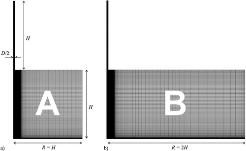
Besides domain size, results were also tested for grid convergence by varying the number of grid cells. Thus, two sets of grid density were built by more than doubling the number of cells in each direction x and r, corresponding to a linear grid ratio of ∼2.03. Thus, the coarsest meshes A1 and B1 (Figure 2) counted a total of ∼31 and ∼33 thousand cells, respectively, whereas the finest meshes A2 and B2 (not shown in Figure 2) counted a total of ∼128 and ∼135 thousand cells, respectively.

Uncertainty estimation

In the validation part of this study, results were compared to experimental and numerical data on immersed jets (Shademan et al. 2016, among other studies). Additionally, numerical uncertainties in terms of grid convergence were quantified using the grid convergence index (GCI) for the fine grid solution, as detailed in Roache (1994): (6) $$\mathit{GCI}\mathrm{ }\left[\text{fine grid}\right]=3\mathrm{ }\left|\left|\frac{f_1-f_2}{f_2}\right|\right|/({\mathit{Gr}}^{\mathit{Np}}-1)$$(6) where $f_1$ and $f_2$ are the coarse and fine grid solutions, respectively,$\mathrm{ }\mathit{Gr}$ is the grid ratio (presently, $\mathit{Gr}$ ≈ 2.03) and$\mathrm{ }\mathit{Np}\mathrm{ }$is the order of the numerical method ($\mathit{Np}$ = 2).

Results and discussion

Grid verification and method validation

Before considering scaling of waterjet adhesion strength testing, the current numerical results for the immersed waterjet must be verified for grid convergence. This was achieved using the GCI (Roache 1994), and comparison of profiles of main variables. Further, the current numerical method was validated against results from previous experimental and numerical studies.

For grid verification, GCI values are presented in Table 3 for local wall surface forces, namely the stagnation pressure, p_s, and the maximum wall shear stress, τ_w,max. A GCI equal to or lower than 3.3% was achieved, representing the approximate uncertainty associated with grid doubling ($\mathit{Gr}$ = 2) using a second order numerical method (Roache 1994). This provides confidence that current results for the fine grids are practically grid-independent. Even though a higher number of grids would be required for verifying the asymptotic behaviour of current results, the relatively high grid ratio ($\mathit{Gr}$ ≈ 2.03) and the profile comparisons between grids, as discussed below, provide further confidence in terms of grid convergence.

Table 3. Grid convergence index (GCI) for the fine grid solution (stagnation pressure p_s and maximum wall shear stress τ_w,max), calculated according to Equation 6(6) $$\mathit{GCI}\mathrm{ }\left[\text{fine grid}\right]=3\mathrm{ }\left|\left|\frac{f_1-f_2}{f_2}\right|\right|/({\mathit{Gr}}^{\mathit{Np}}-1)$$(6) , based on Roache (1994), for the validation case (D = 0.01 m, Re = 28,000).

Turbulence model and domain size	ps [Pa]			τw,max [Pa]
	f1	f2	GCI	f1	f2	GCI
SST, grid A	456	446	2.2%	6.13	6.22	1.3%
SST, grid B	455	445	2.1%	6.12	6.21	1.4%
ReaKEps, grid A	399	413	3.3%	4.40	4.51	2.4%
ReaKEps, grid B	399	404	1.3%	4.40	4.45	1.2%

For validation purposes, several computed variables are next compared against previous experimental and numerical results, namely centreline velocity, radial velocity, wall pressure and wall shear stress.

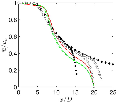
Profiles for centreline velocity $\overline{u}$/u₀ are plotted in Figure 3, starting with $\overline{u}$/u₀ = 1 at the centre of the nozzle exit (x/D = 0), and decaying to $\overline{u}$/u₀ = 0 at the wall (x/D = H/D). Close to the nozzle, at x/D < 6, the current results show an extended region of slow decay, or potential core, compared to the experimental results for a free jet (Giralt, Chia, and Trass 1977). This extended potential core could be due to differences in nozzle design (Xu and Antonia 2002), also affecting the velocity decay further downstream. At x/D > 6, a sharp velocity decay is first observed, which is associated with the entrainment of ambient fluid (Shademan, Balachandar, and Barron 2013). Then, a final sharp decay is observed for x/D > 18, which is associated with the impingement region in the presence of a wall. Compared to the ReaKEps turbulence model, results from the SST model more closely match the experimental observations made by Shademan et al. (2016), obtained at the same stand-off distance H/D = 20 (Figure 3). Additionally, differences between coarse and fine grids are comparatively small (dashed lines compared against solid lines), confirming practical grid independence of the current results. Finally, differences due to domain size are almost unnoticeable, with curves for grids A and B practically overlapping (Figure 3).

Figure 3. Centreline velocity $\overline{u}$/u₀ along the axial length x/D. This study: ▬ ▬ (red) SST Grid A1, ▬ (red) SST Grid A2, ▬ ▬ (black) SST Grid B1, ▬ (black) SST Grid B2, ▬ ▬ (green) ReaKEps Grid A1, ▬ (green) ReaKEps Grid A2, ▬ ▬ (blue) ReaKEps Grid B1, ▬ (blue) ReaKEps Grid B2. Reference experimental studies: –♦– H/D = ∞ (Giralt, Chia, and Trass 1977), △ H/D = 22.0 (Giralt, Chia, and Trass 1977), –○– H/D = 20 (Shademan et al. 2016), ■ H/D = 15.56 (Giralt, Chia, and Trass 1977). Note that results for grids A and B practically overlap.

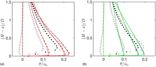
In Figure 4, radial velocities v/u₀ are plotted against distance from the wall (H – x)/D for four radial distances r/D = 0, 1, 2 and 3. The development of the wall boundary layer is observed, and results can be compared to PIV measurements made by Shademan et al. (2016). Although apparently higher slopes in the boundary layer close to the wall are observed in current results compared to PIV measurements of Shademan et al. (2016), the SST model (Figure 4a) performs in qualitatively better agreement with previous results than the ReaKEps model (Figure 4b), considering that the shape of the boundary layer is more closely represented using the former turbulence model.

Figure 4. Radial velocity $\overline{v}$/u₀, at four radial distances, for a) SST model, b) ReaKEps model. This study: ▬ ▬ (red) SST Grid A1, ▬ (red) SST Grid A2, ▬ ▬ (black) SST Grid B1, ▬ (black) SST Grid B2, ▬ ▬ (green) ReaKEps Grid A1, ▬ (green) ReaKEps Grid A2, ▬ ▬ (blue) ReaKEps Grid B1, ▬ (blue) ReaKEps Grid B2. Reference experimental study: ◊ r/D = 0, △ r/D = 1, ■ r/D = 2, × r/D = 3 (Shademan et al. 2016). Note that results for grids A and B practically overlap.

To validate surface forces at the wall, pressure profiles are plotted in Figure 5, whereas wall shear stress profiles are plotted in Figure 6.

Figure 5. Wall pressure p/p_s as a function of radial distance r/r_1/2. This study: ▬ ▬ (red) SST Grid A1, ▬ (red) SST Grid A2, ▬ ▬ (black) SST Grid B1, ▬ (black) SST Grid B2, ▬ ▬ (green) ReaKEps Grid A1, ▬ (green) ReaKEps Grid A2, ▬ ▬ (blue) ReaKEps Grid B1, ▬ (blue) ReaKEps Grid B2. Reference studies: ▬ Beltaos & Rajaratnam (1974) (experimental), ○ Shademan, Balachandar, and Barron (2013) (RANS). Note that results for grids A and B practically overlap.

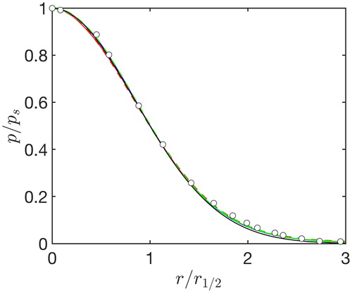
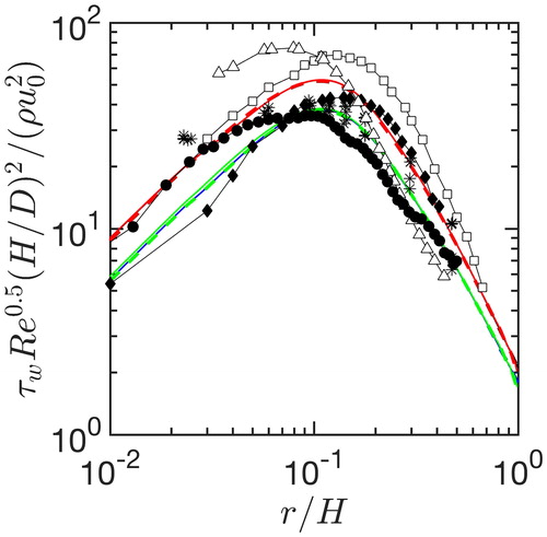
Figure 6. Dimensionless wall shear stress as a function of radial distance. This study: ▬ ▬ (red) SST Grid A1, ▬ (red) SST Grid A2, ▬ ▬ (black) SST Grid B1, ▬ (black) SST Grid B2, ▬ ▬ (green) ReaKEps Grid A1, ▬ (green) ReaKEps Grid A2, ▬ ▬ (blue) ReaKEps Grid B1, ▬ (blue) ReaKEps Grid B2. Reference studies: –□– H/D = 18, experimental (Bradshaw & Love 1961), –◊– H/D = 21.2, experimental (Beltaos & Rajaratnam 1974), * H/D = 16.5, experimental (Hanson, Robinson, and Temple 1990), –△– H/D = 18.5, RANS (Shademan, Balachandar, and Barron 2013), –●– H/D = 20, LES (Shademan et al. 2016). Note that results for grids A and B practically overlap.

Regarding wall pressure, it is observed that the shape of pressure profiles (Figure 5) is in very good agreement with previous studies (Beltaos and Rajaratnam 1974; Shademan, Balachandar, and Barron 2013). Additionally, the obtained stagnation pressure p_s, which is observed at r = 0 for vertically impinging jets (Figure 5), corresponded to 445 and 404 Pa, for the SST and ReaKEps turbulence models, respectively (Table 3, grid B, f₂). These values are within 1.2% and 8.2%, for SST and ReaKEps turbulence models respectively, compared to a reference value of 440 Pa obtained from LES numerical simulation (Shademan et al. 2016).

Regarding wall shear stress profiles (Figure 6), shear stress increases from a theoretical zero at r = 0 (not represented) to a maximum value at r $\approx$ 0.1 H, in agreement with previous experimental studies. The maximum value is followed by a slow decay for higher radii (note the logarithmic scale in Figure 6). Although current results using the SST turbulence model seem to overestimate the dimensionless maximum wall shear stress compared to the LES numerical results from Shademan et al. (2016), there is still considerable spread among previous studies (Figure 6). Compared to the LES numerical results from Shademan et al. (2016), several previous studies on fully developed round jets also suggest somewhat higher dimensionless wall shear stress values (Bradshaw and Love 1961; Beltaos and Rajaratnam 1974; Shademan, Balachandar, and Barron 2013). Finally, the formula from Phares, Smedley, and Flagan (2000), presented above in Equation 3(3) $${\tau }_{w,m}=44.6\frac{\rho {u_0}^2{\mathit{Re}}^{-\frac{1}{2}}}{{\left(H/D\right)}^2}, \mathrm{at}\mathrm{ }r/H =\mathrm{ }0.09$$(3) , also yields a somewhat higher τ_w,max (∼5.25 Pa), which is within 15% from the current SST results (τ_w,max 6.21 Pa, Table 3).

Considering the above, grid B2 (large domain, fine grid) is used from here on, following an approach that minimizes domain error and discretization error, the latter associated with a GCI ≤ 2.1% (Table 3). Additionally, the SST turbulence model was selected, which generally yielded results in somewhat closer agreement with available experimental and numerical work.

Empirical study on scaling parameters

As discussed above, forces acting on a wall under an impinging jet are divided into a normal component and tangential component, associated with wall pressure p and wall shear stress τ_w, respectively. In this section, it is demonstrated that these force components are not linearly correlated to each other, meaning that each force component scales with different flow parameters, contrary to what was suggested in Beltaos and Rajaratnam (1974), and later applied in Finlay et al. (2002).

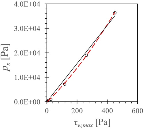
In Figure 7, results for stagnation pressure p_s are plotted against maximum wall shear stress τ_w,max. These results deviate from a linear trend, where p_s increases more rapidly than τ_w,max, approximately following a quadratic function. These results are also backed by previous studies (Figure A1 in Supplementary material), demonstrating that pressure does not scale with shear stress, at least in the case of a round vertically impinging jet.

Figure 7. Simulated stagnation pressure p_s, plotted against simulated maximum wall shear stress τ_w,max. Legend: solid black line – linear regression with zero intercept; dashed red line – second order polynomial regression. Coefficient of determination for linear regression with zero intercept: R²_adj = 0.98331.

As in Equations 1(1) $$p_s=25\frac{\rho {u_0}^2}{{\left(H/D\right)}^2}, \mathrm{at}\mathrm{ }r/H =\mathrm{ }0$$(1) and 2(2) $${\tau }_{w,\mathit{max}}=0.16\frac{\rho {u_0}^2}{{\left(H/D\right)}^2}, \mathrm{at}\mathrm{ }r/H =\mathrm{ }0.14$$(2) , proposed by Beltaos and Rajaratnam (1974), both p_s and τ_w,max are plotted against the scaling parameter ρu₀²/(H/D)² in Figure 8. It is observed that p_s varies linearly with the proposed scaling parameter (Figure 8a), with low level of residuals, <2.5% off the actual simulated pressure values. The obtained slope $m_{p_s}$ = 23.1 (Table 4) compares well with a slope of 25 previously reported in Beltaos and Rajaratnam (1974), though higher slopes closer to $\sim$30 have also been reported elsewhere (Hanson, Robinson, and Temple 1990). In contrast, a linear trend was not observed for τ_w,max (Figure 8b), where residuals are much higher, corresponding to up to >40%. Accordingly, the adjusted coefficient of determination R²_adj is higher for p_s against ρu₀²/(H/D)², with R²_adj = 0.99992, than for τ_w,maxagainst the same scaling parameter, with R²_adj = 0.98323.

Figure 8. Simulated wall surface forces as a function of ρu₀²/(H/D)²: (a) stagnation pressure p_s, and (b) maximum wall shear stress τ_w,max. Left-hand side: solid black line – linear regression with zero intercept; dashed red line – second order polynomial regression. Right-hand side: residuals correspond to the linear regression with zero intercept. Coefficient of determination for linear regressions with zero intercept: R²_adj (p_s) = 0.99992, R²_adj (τ_w,max) = 0.98323.

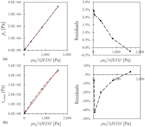
Table 4. Slope, m, and adjusted correlation coefficients, R²_adj, for stagnation pressure p_s and maximum wall shear stress τ_w,max, as functions of different scaling parameters.

Scaling parameter	Slope m (R^2adj), this study		Slope m (R^2adj), reference
	ps	τw,max	ps	τw,max
ρu0^2/(H/D)^2	23.1 (0.99992)	0.294 (0.98323)	27.7 (0.99423)	0.150 (0.95665)
ρu0^2Re^−1/2/(H/D)^2	4,341 (0.95645)	55.7 (0.99265)	7,380 (0.94964)	40.9 (0.96175)
ρu0^2Re^−0.3159/(H/D)^2	634 (0.98326)	8.11 (0.99998)	949 (0.97509)	5.22 (0.96996)

Footnote to Table 4: Reference studies: Bradshaw & Love 1961; Beltaos & Rajaratnam 1974; Hanson, Robinson, and Temple 1990; Shademan, Balachandar, and Barron 2013; Shademan et al. 2016 (please refer to Supplemental material).

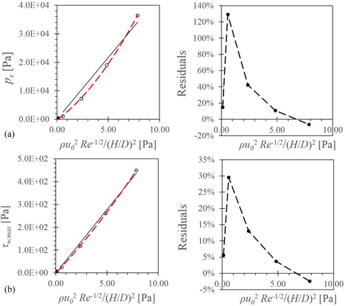
As an alternative to the scaling parameter ρu₀²/(H/D)², Phares, Smedley, and Flagan (2000) scale τ_w,max with ρu₀²Re^−1/2/(H/D)², including Reynolds number based on nozzle diameter Re. The proposed exponent −1/2 is based on the assumption of a laminar boundary layer in the impingement region. In Figure 9, both p_s and τ_w,max are plotted against ρu₀²Re^−1/2/(H/D)². For this scaling parameter, the situation is now reversed, with τ_w,max scaling better than p_s: residuals are larger for p_s, up to more than 120% (Figure 9a), compared to <30% residuals for τ_w,max against ρu₀²Re^−1/2/(H/D)² (Figure 9b). In agreement with a better visual fit and lower residuals for τ_w,max (Figure 9), an R²_adj = 0.99265 is obtained for τ_w,max, higher than R²_adj = 0.95645 obtained for p_s (Table 4). However, there seems to be a slight curvature in τ_w,max against ρu₀²Re^−1/2/(H/D)² (Figure 9b), suggesting further improvements in terms of fit can be achieved.

Figure 9. Simulated wall surface forces as a function of ρu₀²/Re^−1/2/(H/D)²: (a) stagnation pressure p_s, and (b) maximum wall shear stress τ_w,max. Left-hand side: solid black line – linear regression with zero intercept; dashed red line – second order polynomial regression. Right-hand side: residuals correspond to the linear regression with zero intercept. Coefficient of determination for linear regressions with zero intercept: R²_adj (p_s) = 0.95645, R²_adj (τ_w,max) = 0.99265.

In order to further improve the above fit for τ_w,max against ρu₀²Re^−a/(H/D)², the exponent a for the Reynolds number was optimized using Microsoft Excel^® 2013’s Solver tool (Frontline Systems Inc., Incline Village, NV, USA, www.solver.com), maximizing the correlation coefficient R²_adj. For the current numerical results, an exponent corresponding to −0.3159 could thus be obtained, and results are plotted in Figure 10 for p_s and τ_w,max against ρu₀²Re^−0.3159/(H/D)². An almost perfect fit was obtained for τ_w,maxagainst ρu₀²Re^−0.3159/(H/D)², with R²_adj practically equal to unity (Table 4, R²_adj = 0.99998) and residuals within 4% (Figure 10b). Results for p_sagainst ρu₀²Re^−0.3159/(H/D)² were also improved when compared to p_sagainst ρu₀²Re^−1/2/(H/D)², with decreased residuals (Figure 10a, <80% compared to >120%) and an increased R²_adj (Table 4, R²_adj = 0.98326 compared to 0.95645).

Figure 10. Simulated wall surface forces as a function of ρu₀²/Re^−0.3159/(H/D)²: (a) stagnation pressure p_s, and (b) maximum wall shear stress τ_w,max. Left-hand side: solid black line – linear regression with zero intercept; dashed red line – second order polynomial regression. Right-hand side: residuals correspond to the linear regression with zero intercept. Coefficient of determination for linear regressions with zero intercept: R²_adj (p_s) = 0.98326, R²_adj (τ_w,max) = 0.99998.

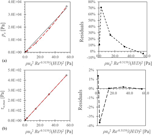
Overall, the current numerical results, backed by previous experimental studies, suggest that stagnation pressure p_s and maximum wall shear stress τ_w,maxscale with different parameters: p_s scales better with ρu₀²/(H/D)², scoring R²_adj = 0.99992, and τ_w,maxscales better with ρu₀²Re^−0.3159/(H/D)², scoring R²_adj = 0.99998 (Table 4).

Implications for adhesion strength testing and hull cleaning/grooming

The scaling of normal and tangential forces with different flow parameters has several implications for adhesion-strength testing with calibrated waterjets. Future waterjet apparatuses are envisioned to determine the adhesion strength of marine microfouling as a starting point for matching cleaning forces on commercial devices to the adhesion strength of fouling, and thus minimizing the wear and damage inflicted on hull coatings during in-water cleaning.

First, there is a need to report adhesion strength of microfouling as a combination of both stagnation pressure and maximum wall shear stress, since both pressure and wall shear stress may be involved in the cleaning process (Finlay et al. 2002). Thus, the current results suggest the following separate scaling relations for each of wall pressure and shear stress, respectively: (7) $$p_s=m_{p_s}\frac{\rho {u_0}^2}{{\left(H/D\right)}^2} \left[{\text{N m}}^{-2}\right]$$(7) (8) $${\tau }_{w,\mathit{max}}=m_{{\tau }_{w,\mathit{max}}}\frac{\rho {u_0}^2{\mathit{Re}}^{-0.3159}}{{\left(H/D\right)}^2} \left[{\text{N m}}^{-2}\right]$$(8) where, for slopes m, there is still some discrepancy between current numerical results and those obtained from reference studies (Table 4). These differences could be due to the current assumption of turbulent flow in the entire simulated domain, which might contribute to an overestimation of shear stress. Thus, depending on the method used in the future for calculating cleaning forces for hull cleaning devices, the appropriate slopes in Table 4 must be considered in matching those forces to adhesion strength obtained with calibrated waterjets: for example, if a CFD approach based on the present method is applied to a particular device used in hull cleaning, slopes $m_{p_s}$= 23.1 and $m_{{\tau }_{w,\mathit{max}}}$= 8.11 would enable a direct comparison, whereas if an experimental method is used (eg electrochemical method), slopes $m_{p_s}$= 27.7 and $m_{{\tau }_{w,\mathit{max}}}$= 5.22 would be more appropriate. Nevertheless, it should be noted that the current numerical results agree with experimental and numerical results from previous literature (see Supplemental material) in that the best fit is obtained using scaling parameters given in Equations 7(7) $$p_s=m_{p_s}\frac{\rho {u_0}^2}{{\left(H/D\right)}^2} \left[{\text{N m}}^{-2}\right]$$(7) and 8(8) $${\tau }_{w,\mathit{max}}=m_{{\tau }_{w,\mathit{max}}}\frac{\rho {u_0}^2{\mathit{Re}}^{-0.3159}}{{\left(H/D\right)}^2} \left[{\text{N m}}^{-2}\right]$$(8) .

In previous studies using water-in-air jets (Finlay et al. 2002; Hunsucker and Swain 2016), results cannot be directly used for selecting in-water cleaning forces. Thus, future adhesion strength tests should be conducted using immersed waterjets, so that the above relations remain valid.

It should also be noted that immersed waterjets, rather than water-in-air jets, more closely resemble the type of flow encountered in in-water commercial hull cleaning with waterjets. However, the above relationships were obtained assuming an axisymmetric flow over a flat surface, which can only be replicated under controlled testing conditions, such as bench-scale calibrated waterjet testing apparatuses where angle and position are accurately set by a positioning system (Finlay et al. 2002). Therefore, these relations do not apply to more complex flows found on full-scale commercial cleaning/grooming devices using waterjets, for which tailored experimental or CFD studies are required. In those cases, non-axisymmetric effects need to be considered, such as local curvature of the hull, any significant translational motion of the nozzle relative to the wall (eg high-speed rotating nozzles, and translation speed of cleaning devices over the hull), and possible interaction between individual jets in multi-jet devices.

Another relevant aspect in Equations 7(7) $$p_s=m_{p_s}\frac{\rho {u_0}^2}{{\left(H/D\right)}^2} \left[{\text{N m}}^{-2}\right]$$(7) and 8(8) $${\tau }_{w,\mathit{max}}=m_{{\tau }_{w,\mathit{max}}}\frac{\rho {u_0}^2{\mathit{Re}}^{-0.3159}}{{\left(H/D\right)}^2} \left[{\text{N m}}^{-2}\right]$$(8) is that the wall shear stress, contrary to pressure, is also a function of Reynolds number and therefore a function of fluid viscosity. This dependency on viscosity means that wall shear stress is more sensitive to temperature changes than the stagnation pressure: for example, decreasing the fluid temperature from 20 °C to 5 °C leads to an increase in fluid viscosity ν of ∼50% and a corresponding increase in τ_w,max of ∼14% (Equation 8(8) $${\tau }_{w,\mathit{max}}=m_{{\tau }_{w,\mathit{max}}}\frac{\rho {u_0}^2{\mathit{Re}}^{-0.3159}}{{\left(H/D\right)}^2} \left[{\text{N m}}^{-2}\right]$$(8) ), whereas p_s increases only ∼0.2% due to a marginal increase in water density (Equation 7(7) $$p_s=m_{p_s}\frac{\rho {u_0}^2}{{\left(H/D\right)}^2} \left[{\text{N m}}^{-2}\right]$$(7) ). This dependency on temperature means that fluid temperature must be known in both adhesion-strength tests and full-scale hull cleaning/grooming in order to match tangential forces. To a lesser extent, salinity can also be shown to affect both pressure and shear forces within ∼4%, for salinity 35 ppt compared to freshwater (∼0 ppt).

In addition to temperature, water quality is also likely to affect cleaning efficacy as particulate matter suspended in the cleaning fluid (filtered seawater) might lead to increased abrasion to the surface being cleaned compared to distilled/pure water. This topic is certainly worth further investigation and is relevant to previous research on the cleaning efficacy of cavitating jets (Kalumuck et al. 1997).

Finally, adhesion strength results are expected to be dependent on the time interval allowed for the waterjet to exert an effect on the surface. Previous research clearly demonstrated that the threshold shear stress for particle removal increases with increasing translation speed (Phares, Smedley, and Flagan 2000). Such time dependency may hinder a direct comparison to hull cleaning devices, which typically operate at translation speeds that are several orders of magnitude higher (from Noordstrand and Cornelis Petrus Maria 2013; Andersen 2012: translation speeds of 5–50 m s⁻¹) than those speeds used in adhesion strength testing (Finlay et al. 2002: translation speeds in order of 0.01 m s⁻¹). Therefore, dependency on translation speed warrants further research, namely by varying translation speed in future adhesion strength testing and thus deriving a correction for time dependency.

Conclusions

An absolute scale for the adhesion strength of hull microfouling would be useful to optimize the design and operation of in-water hull cleaning devices. This would enable minimization of wear and damage to in-water ship hull coatings during in-water cleaning, while still being effective at the removal of early stages of marine growth.

For several reasons, pressure and shear forces previously reported in the literature on the adhesion strength of marine microfouling cannot be used as an absolute measure of adhesion strength. The reasons include the use of water-in-air jets instead of immersed jets, as well as inaccurate semi-empirical formulae and effects of other parameters, such as temperature and translation speed.

This study shows that the tangential and normal forces under immersed calibrated waterjets scale with different flow parameters, and these components should therefore be calculated separately. Semi-empirical formulae are derived, which better represent the available experimental and numerical data on impinging jets, and thus will enable more accurate reporting of adhesion strength from immersed calibrated waterjets.

Based on both present results and those from the literature on immersed round jets, scaling parameters ρu₀²/(H/D)² and ρu₀²Re^−0.3159/(H/D)² are suggested for stagnation pressure p_s and maximum wall shear stress τ_w,max, respectively. In order to use these parameters in an absolute scale for marine microfouling adhesion strength, time dependency of cleaning results should be addressed in future research.

Nomenclature
a	=	empirically fitted parameter [–]
D	=	nozzle diameter [m]
f	=	numerical solution (generic variable)
GCI	=	grid convergence index
Gr	=	grid ratio, number of cells fine grid/number of cells coarse grid, in each direction
H	=	stand-off distance [m]
m	=	slope in semi-empirical relations
Np	=	order of the numerical method
p	=	hydrodynamic pressure [Pa]
Q	=	nozzle flowrate [m3 s−1]
R	=	radial length of the domain [m]
R2adj	=	adjusted coefficient of determination (Montgomery 2013, p. 464)
Re	=	Reynolds number based on nozzle diameter, Re = u0D/ν [–]
x, r	=	axial and radial coordinates [m]
r1/2	=	radial distance where wall pressure p = ½ ps [m]
$\overline{u}, \overline{v}$	=	time-averaged axial and radial local velocities [m s–1]
u0	=	mean velocity at the nozzle, u0 = 4Q/(πD2) [m s−1]
ν	=	kinematic viscosity of the fluid [m2 s−1]
ρ	=	density of the fluid [kg m−3]
τw	=	wall shear stress [Pa]

subscript
max	=	maximum
s	=	stagnation point, ie (x, r) = (H, 0)
1	=	coarse grid
2	=	fine grid

superscript
$\mathrm{\prime }$	=	time-dependent component

Abbreviations
AF	=	antifouling coatings
AFM	=	atomic force microscopy
CFD	=	computational fluid dynamics
FR	=	foul-release coatings
JET	=	jet erosion test
PIV	=	particle image velocimetry
RANS	=	Reynolds averaged Navier–Stokes
ReaKEps	=	realizable k-ε turbulence model
SST	=	Shear stress transport k-ω turbulence model

Acknowledgements

The authors would like to acknowledge early discussions on the topic with Professor Rickard Bensow and Assistant Professor Arash Eslamdoost (Chalmers University of Technology). Acknowledgements are also due to Dr Libby Schweber (University of Reading) for comments on language and the readability of an earlier version of the manuscript, and also to three anonymous reviewers, for their valuable comments.

Disclosure statement

No potential conflict of interest was reported by the authors.

Additional information

Funding

This study was prepared within the project COMPLETE - Completing management options in the Baltic Sea region to reduce risk of invasive species introduction by shipping [#R069]. The project is co-financed by the European Union’s funding Programme Interreg Baltic Sea Region (European Regional Development Fund).

References

- Ackerman JD, Ethier CR, Allen DG, Spelt JK. 1992. Investigation of zebra mussel adhesion strength using rotating disks. J Environ Eng. 118:708–724. doi: 10.1061/(ASCE)0733-9372(1992)118:5(708)
- Alekseenko SV, Markovich DM. 1994. Electrodiffusion diagnostics of wall shear stresses in impinging jets. J Appl Electrochem. 24:626–631. doi: 10.1007/BF00252087
- Andersen R. 2012. A surface-cleaning device and vehicle. International Patent WO 2012/074408 A2.
- Beltaos S, Rajaratnam N. 1974. Impinging circular turbulent jets. ASCE J Hydraul Div. 100:1313–1328.
- Bradshaw P, Love EM. 1961. The normal impingement of a circular air jet on a flat surface. Reports and Memoranda No. 3205. London (UK).
- Callow JA, Crawford S. A, Higgins MJ, Mulvaney P, Wetherbee R. 2000. The application of atomic force microscopy to topographical studies and force measurements on the secreted adhesive of the green alga Enteromorpha. Planta. 211:641–647. doi: 10.1007/s004250000337
- Davidson IC, Scianni C, Hewitt C, Everett R, Holm ER, Tamburri M, Ruiz GM. 2016. Mini-review: assessing the drivers of ship biofouling management – aligning industry and biosecurity goals. Biofouling. 32:411–428. doi: 10.1080/08927014.2016.1149572
- Finlay JA, Callow ME, Schultz MP, Swain GW, Callow JA. 2002. Adhesion strength of settled spores of the green alga Enteromorpha. Biofouling. 18:251–256. doi: 10.1080/08927010290029010
- Ghaneeizad SM, Atkinson JF, Bennett SJ. 2015. Effect of flow confinement on the hydrodynamics of circular impinging jets: implications for erosion assessment. Environ Fluid Mech. 15:1–25. doi: 10.1007/s10652-014-9354-3
- Giralt F, Chia C-J, Trass O. 1977. Characterization of the impingement region in a axisymmetric turbulent jet. Ind Eng Chem Fund. 16:21–28. doi: 10.1021/i160061a007
- Hanson GJ, Cook KR. 2004. Apparatus, test procedures, and analytical methods to measure soil erodibility in situ. Appl Eng Agric. 20:455–462.
- Hanson GJ, Robinson KM, Temple DM. 1990. Pressure and stress distributions due to a submerged impinging jet. Proceedings of the 1990 National Conference ASCE, Vol. 1. pp. 525–530. San Diego, CA, Jul 30–Aug 3, 1990.
- Hearin J, Hunsucker KZ, Swain G, Stephens A, Gardner H, Lieberman K, Harper M. 2015. Analysis of long-term mechanical grooming on large-scale test panels coated with an antifouling and a fouling-release coating. Biofouling. 31:625–638. doi: 10.1080/08927014.2015.1081687
- Holm ER, Haslbeck EG, Horinek AA. 2003. Evaluation of brushes for removal of fouling from fouling-release surfaces, using a hydraulic cleaning device. Biofouling. 19:297–305. doi: 10.1080/0892701031000137512
- Hunsucker KZ, Swain GW. 2016. In situ measurements of diatom adhesion to silicone-based ship hull coatings. J Appl Phycol. 28:269–277. doi: 10.1007/s10811-015-0584-7
- Hunsucker KZ, Vora GJ, Hunsucker JT, Gardner H, Leary DH, Kim S, Lin B, Swain G. 2018. Biofilm community structure and the associated drag penalties of a groomed fouling release ship hull coating. Biofouling. 7014:1–11.
- IMO 2011. Guidelines for the control and management of ships’ biofouling to minimize the transfer of invasive aquatic species. In: Resolut MEPC207(62). London (UK); p. 1–25.
- Jambunathan K, Lai E, Moss MA, Button BL. 1992. A review of heat transfer data for single circular jet impingement. Int J Heat Fluid Flow. 13:106–115. doi: 10.1016/0142-727X(92)90017-4
- Kalumuck KM, Chahine GL, Frederick GS, Aley PD. 1997. Development of a DynaJet(TM) cavitating water jet cleaning tool for underwater marine fouling removal. In: Hashish M, editor. 9th Am Waterjet Conf. Dearborn, Michigan: Waterjet Technology Association; p. 541–554.
- Kataoka K, Mizushina T. 1974. Local enhancement of the rate of heat transfer in an impinging round jet by free-stream turbulence. In: Kaigi NG, Kyōkai KK, Gakkai NK, editors. Proc 5th Int Heat Transf Conf. Tokyo (Japan); p. 305–309.
- Larsson L, Raven HC. 2010. Governing equations. In: Paulling JR, editor. Princ Nav Archit Ser - Sh Resist Flow. Jersey City (NJ); p. 5–9.
- Malone JA. 1980. Effects of hull foulants and cleaning/coating practices on ship performace and economics. Trans Soc Nav Archit Mar Eng. 88:75–101.
- Montgomery DC. 2013. Design and analysis of experiments. 8th edition. Singapore: John Wiley & Sons, Inc.
- Morrisey D, Woods CMC. 2015. In-water cleaning technologies: Review of information Prepared for Ministry for Primary Industries [Internet]. Wellington (New Zealand). Available from: http://www.mpi.govt.nz/news-and-resources/publications/
- Munk T, Kane D, Yebra DM. 2009. The effects of corrosion and fouling on the performance of ocean-going vessels: a naval architectural perspective. In: Hellio C, Yebra D, editors. Adv Mar antifouling coatings Technol. Oxford (UK): Woodhead Publishing Limited; p. 148–176.
- Naval Sea Systems Command. 2006. Chapter 081 – Water-borne underwater hull cleaning of Navy ships. In: Nav Ship’s Tech Man. Washington DC.
- Noordstrand AM, Cornelis Petrus Maria DV. 2013. Cleaning head for cleaning a surface, device comprising such cleaning head, and method of cleaning, International Patent WO 2013/154426 A1.
- Oliveira D, Granhag L. 2016. Matching forces applied in underwater hull cleaning with adhesion strength of marine organisms. JMSE. 4:66–78. doi: 10.3390/jmse4040066
- Phares DJ, Smedley GT, Flagan RC. 2000. The wall shear stress produced by the normal impingement of a jet on a flat surface. J Fluid Mech. 418:351–375. doi: 10.1017/S002211200000121X
- Poreh M, Tsuei YG, Cermak JE. 1967. Investigation of a turbulent radial wall jet. J Appl Mech. 34:457–463. doi: 10.1115/1.3607705
- Roache PJ. 1994. Perspective: a method for uniform reporting of grid refinement studies. J Fluids Eng. 116:405–413. doi: 10.1115/1.2910291
- Schiff K, Diehl D, Valkirs A. 2004. Copper emissions from antifouling paint on recreational vessels. Mar Pollut Bull. 48:371–377. doi: 10.1016/j.marpolbul.2003.08.016
- Schultz MP, Bendick JA, Holm ER, Hertel WM. 2011. Economic impact of biofouling on a naval surface ship. Biofouling. 27:87–98. doi: 10.1080/08927014.2010.542809
- Schultz MP, Finlay JA, Callow ME, Callow JA. 2000. A turbulent channel flow apparatus for the determination of the adhesion strength of microfouling organisms. Biofouling. 15:243–251. doi: 10.1080/08927010009386315
- Schultz MP, Finlay JA, Callow ME, Callow JA. 2003. Three models to relate detachment of low form fouling at laboratory and ship scale. Biofouling. 19 Suppl:17–26.
- Schultz MP. 2007. Effects of coating roughness and biofouling on ship resistance and powering. Biofouling. 23:331–341. doi: 10.1080/08927010701461974
- Shademan M, Balachandar R, Barron RM. 2013. CFD analysis of the effect of nozzle stand-off distance on turbulent impinging jets. Can J Civ Eng. 40:603–612. doi: 10.1139/cjce-2012-0199
- Shademan M, Balachandar R, Roussinova V, Barron R. 2016. Round impinging jets with relatively large stand-off distance. Phys Fluids. 28:075107. doi: 10.1063/1.4955167
- Swain GW, Schultz MP. 1996. The testing and evaluation of non-toxic antifouling coatings. Biofouling. 10:187–197. doi: 10.1080/08927019609386279
- Tribou M, Swain G. 2017. The effects of grooming on a copper ablative coating: a six year study. Biofouling. 33:494–504. doi: 10.1080/08927014.2017.1328596
- Tribou M, Swain GW. 2015. Grooming using rotating brushes as a proactive method to control ship hull fouling. Biofouling. 31:309–319. doi: 10.1080/08927014.2015.1041021
- Wu W, Banyassady R, Piomelli U. 2016. Large-eddy simulation of impinging jets on smooth and rough surfaces. J Turbul. 17:847–869. doi: 10.1080/14685248.2016.1181761
- Xu G, Antonia RA. 2002. Effect of initial conditions on the temperature field of a turbulent round free jet. Int Commun Heat Mass Transf. 29:1057–1068. doi: 10.1016/S0735-1933(02)00434-7
- Yebra DM, Kiil S, Dam-Johansen K. 2004. Antifouling technology - Past, present and future steps towards efficient and environmentally friendly antifouling coatings. Prog Org Coatings. 50:75–104. doi: 10.1016/j.porgcoat.2003.06.001