Two-dimensional core-softened model with water like properties: solvation of non-polar solute

ABSTRACT

Monte Carlo simulations and integral equation theory were used to study the thermodynamics and structure of mixture of particles interacting through the smooth version of Stell–Hemmer interaction and non-polar particles interacting through Lennard–Jones interaction in two dimensions. The theoretical results are tested against the Monte Carlo computer simulations. Very good agreement between the integral equation theory results and exact computer simulations is obtained. We showed that some versions of the integral equation theory completely fail to predict structure of such system at some state points so caution has to be taken when applying them but in comparison with results for pure component results are better. We also checked how position of critical point changes with content of non-polar particles.

KEYWORDS:

• Monte Carlo
• core-softened model
• critical point

1. Introduction

The two-dimensional (2D) fluids receive in general less theoretical attention as three-dimensional (3D) fluids [1–7]. One of the reasons is that they were in the beginning considered as less interesting, supposedly not being a good representation of real systems. This is not completely true. If molecules of a fluid are confined between the parallel plates, separated for less than two molecular diameters, then the system effectively behaves as 2D. Examples of such systems are monolayers adsorbed on solid substrates [8, 9] or surfactant adsorbed on an air/water interface. The 2D fluids are interesting also from pure theoretical point of view. One aspect of particular importance in their behaviour is the effect of low dimensionality on phase transitions [1, 10–12]. Experimental studies [13, 14] of the adsorption of krypton at low pressures on exfoliated graphite and graphitised carbon black indicated that the adsorbed molecules in many ways are qualitatively similar to the 2D fluid. So on the one hand, 2D fluids can be considered as a simple representation of the liquid phase adsorbed at a solid surface where the lateral interaction prevail and are often used as a coherency test for theories initially developed for the realistic 3D systems. In addition, the 2D models can often be more easily evaluated numerically than their 3D counterparts, especially for computer simulations. The main reason for our interest in 2D systems lies in fact that computer simulations are much less time consuming (100 of particles in 2D is equivalent to 1000 particles in 3D) in 2D than in 3D and results can be easily visualized [15–19]. The 2D Lennard–Jones (LJ) fluid can be, for example, used as a reference system for calculations of the properties of the 2D model of water [17]. This model, also called Mercedes–Benz model of water, was originally proposed by Ben-Naim [20] and later modified and extensively studied by Dill, Haymet and others [15, 16]. The model serves as simplified representation of water and its behaviour when in bulk (pure water) or in mixture with hydrophobic or polar solutes [15, 16].

Water is the most important liquid for life and industry so it is crucial to understand its physical and chemical properties. Water is different when comparing to simpler liquids [21–23]. It has many anomalous properties. The most known are: (i) an increase in the volume of water upon freezing, (ii) an increased density of liquid water in the range from 0${}^{\circ }\mathrm{C}$ up to approximately 4${}^{\circ }\mathrm{C}$ at ambient pressure, (iii) high heat capacity and surface tension, and (iv) minimum in the compressibility vs. temperature. Also as a solvent, water also has some unusual properties: for non-polar solutes, a large entropy that opposes the solvation at room temperature and a large heat capacity of transfer. Water's complexity is due to its strong orientation-dependent hydrogen bonding and intermolecular associations.

There are two different mechanisms to explain the anomalous properties. Between some molecules, we have an angle-dependent interactions (oriented hydrogen bonding in water, tetrahedral bonding in silica) [24–26]. These interactions can result in density maximum or liquid–liquid phase transition [24] because of the competition between tetrahedral order (low density) and translational order (high density). A spherical symmetric potential with two characteristic lengths also exhibit the anomalous properties listed above. An example are core-softened potentials, originally proposed by Stell and Hemmer in 1970 [27]. These potentials have a second critical point in addition to the standard liquid–gas critical point, when interaction potentials have region of negative curvature. It had been shown before that the core-softened and similar potentials can reproduce various fluid anomalies, typical of water [24, 28], such as silica [24], silicon [29], and BeF${}_2$ [30]. Such potentials were also used to study the single-component liquid metal systems [31–35]. After the liquid–liquid phase transition was suggested as an explanation for water's anomalous properties by Poole et al. [36], there was an increase in the interest of studies of such transitions. Various studies have been done to understand the liquid–liquid phase transition and the associated properties [37–39,43–45]. Franzese et al. [40] showed that the reason for the liquid–liquid phase transition and its critical point might be due to the potential with two characteristic distances (hard core and soft core). In their work, they reported the existence of the low-density liquid phase and the high-density liquid phase in a 3D model, using molecular dynamics simulations.

In the present contribution, we study the thermodynamic and structural properties of mixtures of particles interacting through the smooth version of Stell–Hemmer interaction and non-polar particles interacting through LJ interaction in 2D. We checked if the integral equation theory (IET) can be applied effectively for such systems. The IET provides us with a fast and easy-to-implement method of calculating pair distribution functions and thermodynamic properties from know pair distribution functions. IET also allows rather quick calculation of properties along the isotherms or isochores comparing to computer simulations, but it also has drawbacks. It is based on approximations which can lead to convergence problems and even wrong results. Caution must, therefore, be exercised when using IET with a particular closure. In general, results provided by IET in 2D are not that good as in 3D. For example, results for 2D MB model [17] are not as good as for 3D MB model of water [41,42].

This paper is organised as follows. First, we present the core-softened model. In the next section, we present details of the Monte Carlo simulation and IET with different closure relations. In the Results section, we first provide a comparison of pair correlation functions calculated from various IET approximations and those obtained from MC simulations as well as comparison of the thermodynamic properties. In addition, we show Monte Carlo results how critical point moves when more and more non-polar component is added to the system.

2. Model

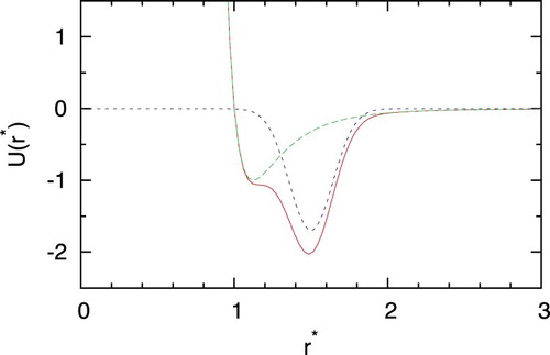
The system was composed with two kinds of particles. For solvent particles, we use the smooth version of the core-softened potential proposed by Scala et al. [45]. The interaction potential $U_{11}\left(r\right)$ is calculated by adding a Gaussian well to the LJ part of the potential and is calculated as (1) $U_{11}\left(r\right)=U_{11}^{LJ}\left(r\right)+U_G\left(r\right),$(1)

where $U_{11}^{LJ}\left(r\right)$ is the standard LJ potential and is defined as (2) $U_{ij}^{LJ}\left(r\right)=4{ϵ}_{ij}\left({\left(\frac{{\sigma }_{ij}}{r}\right)}^{12}-{\left(\frac{{\sigma }_{ij}}{r}\right)}^6\right).$(2) ${ϵ}_{ij}$ denotes the well-depth and ${\sigma }_{ij}$ the contact parameter of LJ potential between particles of type i and type j. Type 1 means solvent and type 2 solute particle. The Gaussian part of the interaction is (3) $U_G\left(r\right)=-\lambda {ϵ}_{11}\exp \left(-a{\left(\frac{r-r_0}{{\sigma }_{11}}\right)}^2\right).$(3) For the sake of comparison with the previous studies, we adopt the units and values of model parameters as used before by Scala et al. [45]. We use ${ϵ}_{11}=$1.0, ${\sigma }_{11}=$1.0, $\lambda =$1.7, $a=$25.0, $r_0=$ 1.5${\sigma }_{11}$. Figure 1 shows the shape of this smooth version of the core-softened potential. For solute–solvent and solute–solute interactions, we used standard LJ potential. The standard Lorentz–Berthelot rules [46] were applied in calculating the solute–solvent and solute–solute interactions as the solute size parameter ${\sigma }_{22}^{LJ}$ was changed from 0.2 ${\sigma }_{11}$ to 4.0 ${\sigma }_{11}$. The LJ potential well depth was fixed at ${ϵ}_{11}$ for all LJ interactions.

Figure 1. The solvent–solvent interaction $U\left(r\right)$ (solid line), the LJ contribution (long dashed line) and the Gaussian part (dashed line).

3. Monte Carlo simulation details

To obtain thermodynamic and structural properties of the mixture of core-softened and LJ particles, we applied the Monte Carlo simulation method in the isothermal-isobaric (NpT) and in the canonical (NVT) ensembles. NVT simulations were done to get structure, while NpT and NVT to get thermodynamics. At each step, displacements of random particles (solute or solvent) in the x, y coordinates were chosen randomly. We used the periodic boundary conditions and the minimum image convention to mimic an infinite system of particles. Starting configurations were selected at random. In NpT ensemble, after 10 moves of particles on average, an attempt is made to scale the dimensions of the box, and all of its component particles, to hold the pressure constant. Here are some of the simulation details: 2×10${}^5$ moves per particle were needed to equilibrate the system. The statistics were gathered over the next 4×10${}^6$ moves to obtain well-converged results. All simulations were performed with $N=$ 100 to 400 molecules. The thermodynamic and structural properties were calculated as the statistical averages of these quantities over the course of the simulations using standard equations [46].

4. Integral equation theory

The Ornstein–Zernike (OZ) equation, proposed by Leonard Salomon Ornstein and Frits Zernike in 1914 [47], is the main equation in the integral equation theory. The OZ equation relates the total correlation function, $h_{ij}\left(r\right)$, with the direct correlation function $c_{ij}\left(r\right)$ in the form (4) $h_{ij}\left(r_{12}\right)=c_{ij}\left(r_{12}\right)+\sum _k{\rho }_k\int c_{ik}\left(r_{13}\right)h_{kj}\left(r_{32}\right)\mathrm{d}{\mathbf{r}}_3.$(4) ${\rho }_k$ is the density of particles of type k. The total correlation function between particle of type i and type j, $h_{ij}\left(r\right)$, is related to the pair distribution function, $g_{ij}\left(r\right)$, as $g_{ij}\left(r\right)=h_{ij}\left(r\right)+1$. In order to solve the OZ, we need an additional relation between $h_{ij}\left(r\right)$ and $c_{ij}\left(r\right)$, called the closure relation, which assumes the general form [48] (5) $g_{ij}\left(r\right)=\exp (-\text{β}{U}_{ij}(r)+h_{ij}(r)-c_{ij}(r)+B_{ij}(r\left)\right).$(5) β is the reverse temperature, $\text{β}=\frac{1}{kT}$, $U_{ij}\left(r\right)$ is the interaction potential between particles and $B_{ij}\left(r\right)$ the bridge function, which is an infinite series of irreducible cluster diagrams and is not known. Various approximations are employed for the bridge function. The simplest option is the hypernetted chain (HNC) approximation, which neglects the bridge function ($B_{ij}\left(r\right)=0$), and simplifies the closure relation to [48] (6) $g_{ij}\left(r\right)=\exp (-\text{β}{U}_{ij}(r)+h_{ij}(r)-c_{ij}(r\left)\right).$(6) Another simple approximation was proposed by Percus and Yevick. [49,50] The Percus–Yevick (PY) closure is obtained as linearisation of HNC closure and is written as (7) $g_{ij}\left(r\right)=\exp (-\text{β}{U}_{ij}(r\left)\right)(1+h_{ij}(r)-c_{ij}(r\left)\right).$(7) Several other closures have been developed to address the shortcomings of HNC and PY, especially a narrow region of convergence and inherent thermodynamic inconsistency. The Kovalenko–Hirata closure (KH) [51], constructed to expand the convergence region, takes the following form $h_{ij}\left(r\right)=\left\{\begin{array}{cc}\exp \left(d_{ij}\right(r\left)\right)-1,& d_{ij}\left(r\right)\le 0\\ d_{ij}\left(r\right),& d_{ij}\left(r\right)>0\end{array}\right\}$where $d_{ij}\left(r\right)=-\text{β}{U}_{ij}\left(r\right)+h_{ij}\left(r\right)-c_{ij}\left(r\right)$. We have also implemented the soft mean-spherical approximation (SMSA). In this closure, we divide the LJ part of potential into a short-range reference part $U_{ij}^0\left(r\right)$ and a longer-range perturbation part $U_{ij}^1\left(r\right)$ as suggested elsewhere [52], (8) $U_{ij}^{LJ}\left(r\right)=U_{ij}^0\left(r\right)+U_{ij}^1\left(r\right),$(8)

where $U_{ij}^0\left(r\right)=\left\{\begin{array}{cc}{U}_{ij}^{LJ}\left(r\right)+{ϵ}_{ij}& r\le r_j^m\\ 0& r>r_j^m\end{array}\right.$and $U_{ij}^1\left(r\right)=\left\{\begin{array}{cc}-{ϵ}_{ij}& r\le r_j^m\\ U_{ij}^{LJ}\left(r\right)& r>r_j^m\end{array}\right..$The distance $r_j^m$ that separates these two components is chosen to be at the position of the minimum of the LJ part of the potential function, i.e. $r_j^m=2^{1/6}{\sigma }_{ij}$. The SMSA closure relation is then written in the following form (9) $g_{ij}\left(r\right)=\exp (-\text{β}{U}_{ij}^0(r\left)\right)(1+h_{ij}(r)-c_{ij}(r)-\text{β}(U_{ij}^1\left(r\right)\left)\right).$(9)

The OZ equation together with the closure condition was solved using a direct iteration method. The forward and inverse Bessel–Fourier transforms, needed to couple the correlation functions in real and Fourier spaces, have been performed by the method of Talman [53]. This method allows us to sample efficiently both the rapidly varying part of the correlation functions at small distances and the long-ranged part using a relatively small number of the grid points, n=1024. Knowledge of the pair correlation functions allows us to calculate the thermodynamic properties of interest, including the internal energy and pressure [54,55].

5. Results and discussion

All results are given in reduced units; excess internal energy and temperature are normalised to the LJ interaction parameter ${ϵ}_{11}$ ($E^{\ast }=\frac{E}{{ϵ}_{11}}$, $T^{\ast }=\frac{k_{B}T}{{ϵ}_{11}}$) and the distances are scaled to the characteristic length ${\sigma }_{11}$ ($r^{\ast }=\frac{r}{{\sigma }_{11}}$).

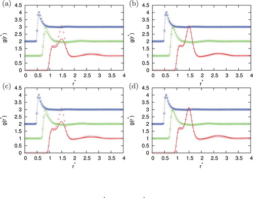
First we checked how well the integral equation with four closure relations, i.e. SMSA, PY, HNC and KH reproduce pair distribution functions that were computed at various potential parameters, densities and temperatures in comparison with Monte Carlo simulations. Figures 2–7 show this comparison for different parameters. There are various asymmetries possible. We study the situation where the second particle is of different size. In Figures 2 and 3, second particle is equal in size (${\sigma }_{11}={\sigma }_{22}$), in Figures 4 and 5, second particle is bigger (${\sigma }_{22}=2.0{\sigma }_{11}$) and in Figures 6 and 7, second particle is smaller (${\sigma }_{22}=0.5{\sigma }_{11}$). Wall-depth was kept equal in all calculations (${ϵ}_{11}={ϵ}_{22}$). In Figures 2–7, we used symbols for Monte Carlo results and lines for IET results. Different correlation functions are plotted shifted for 1 in y direction. Red line and symbols are for $g_{11}\left(r^{\ast }\right)$, green for $g_{12}\left(r^{\ast }\right)$ and blue for $g_{22}\left(r^{\ast }\right)$. Agreement between MC and IET is very good for higher temperatures and all densities where all closures provide results. When the temperature decreases and we are close to phase transition region HNC first and PY later lose the convergence. In the area close to convergence limit we can observe unphysical shapes of correlation functions for HNC closure (see Figure 6). Unphysical shapes also be observed for KH closures at higher densities. The best agreement between MC and IET was observed for PY closure. This was expected since PY work very well for short ranged interactions. The agreement is better in case of higher content of second particles. The PY performs worst in case if we have strong attraction as in the case of the higher content of first particles. In this case, PY closure overestimate LJ peak and underestimate Gaussian peak. The SMSA and KH closures underestimate Gaussian and contact peak for all temperatures and densities. In general, at moderate temperatures theoretical radial distribution functions reproduce only quantitatively simulation results. Positions of main peaks in the radial distribution function are found at correct location but their intensities can be either over- or underestimated.

Figure 2. Comparison of the correlation function for different closures with Monte Carlo simulation results for ${\sigma }_{22}$=1.0, temperature $T^{\ast }=1.5$, ${\rho }_1^{\ast }=0.3$, ${\rho }_2^{\ast }=0.1$. Monte Carlo results are plotted with symbols, and IET by lines. Results are for closures (a) SMSA, (b) PY and (c) KH. Red line and symbols are for $g_{11}\left(r^{\ast }\right)$, green for $g_{12}\left(r^{\ast }\right)$ and blue for $g_{22}\left(r^{\ast }\right)$. Different correlation functions are shifted for 1 in y direction. HNC does not converge for this state point.

Figure 3. Comparison of the correlation function for different closures with Monte Carlo simulation results for ${\sigma }_{22}$=1.0, temperature $T^{\ast }=1.5$, ${\rho }_1^{\ast }=0.1$, ${\rho }_2^{\ast }=0.2$. Monte Carlo results are plotted with symbols, and IET by lines. Results are for closures (a) SMSA, (b) PY, (c) KH and (d) HNC. Legend as in Figure 2.

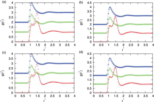
Figure 4. Comparison of the correlation function for different closures with Monte Carlo simulation results for ${\sigma }_{22}$=2.0, temperature $T^{\ast }=1.5$, ${\rho }_1^{\ast }=0.3$, ${\rho }_2^{\ast }=0.05$. Monte Carlo results are plotted with symbols, and IET by lines. Results are for closures (a) SMSA, (b) PY and (c) KH. Legend as in Figure 2. HNC does not converge for this state point.

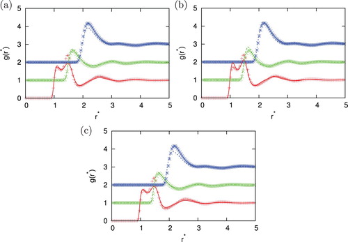
Figure 5. Comparison of the correlation function for different closures with Monte Carlo simulation results for ${\sigma }_{22}$=2.0, temperature $T^{\ast }=1.5$, ${\rho }_1^{\ast }=0.3$, ${\rho }_2^{\ast }=0.15$. Monte Carlo results are plotted with symbols, and IET by lines. Results are for closures (a) SMSA, (b) PY and (c) KH. Legend as in Figure 2. HNC does not converge for this state point.

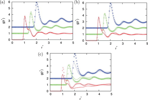
Figure 6. Comparison of the correlation function for different closures with Monte Carlo simulation results for ${\sigma }_{22}$=0.5, temperature $T^{\ast }=1.5$, ${\rho }_1^{\ast }=0.3$, ${\rho }_2^{\ast }=0.1$. Monte Carlo results are plotted with symbols, and IET by lines. Results are for closures (a) SMSA, (b) PY, (c) KH and (d) HNC. Legend as in Figure 2.

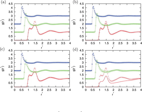
Figure 7. Comparison of the correlation function for different closures with Monte Carlo simulation results for ${\sigma }_{22}$=0.5, temperature $T^{\ast }=1.5$, ${\rho }_1^{\ast }=0.1$, ${\rho }_2^{\ast }=0.2$. Monte Carlo results are plotted with symbols, and IET by lines. Results are for closures (a) SMSA, (b) PY, (c) KH and (d) HNC. Legend as in Figure 2.

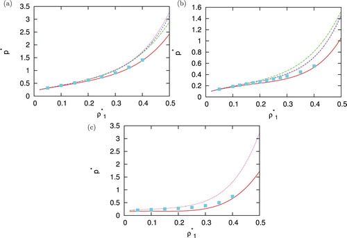
After assessing performances of different closures regarding structures we continued our work with test how well the IET results calculated by virial route [54] can reproduce the internal energy and pressure in comparison with Monte Carlo simulations. This was done for various temperatures, densities of second component and asymmetries of potential. A few examples are plotted in Figures 8 and 9. If line of particular closure is missing means that closure no longer converge here (PY and HNC at lower temperature). The energy is best reproduced by HNC and PY in the situations where convergence is achieved, KH and SMSA are also not that far off. For pressure, no closure is particular superior, and at lower temperatures, SMSA closure has best results which comes as a surprise since SMSA underestimated peaks in pair correlation functions.

Figure 8. Density dependence of internal energy per particle for ${\sigma }_{22}$=1.00 at (a) $T^{\ast }=2.0$, ${\rho }_2^{\ast }=0.1$ (b) $T^{\ast }=1.5$, ${\rho }_2^{\ast }=0.05$ and (c) $T^{\ast }=1.0$, ${\rho }_2^{\ast }=0.2$. Monte Carlo results are plotted with symbols, SMSA with solid red line, PY with long dashed green line, HNC with dashed blue line and KH with dotted pink line.

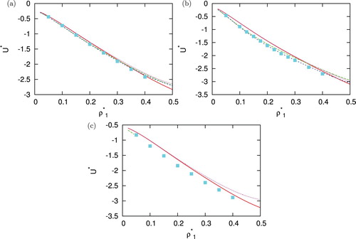
Figure 9. Density dependence of pressure per particle for ${\sigma }_{22}$=1.00 at (a) $T^{\ast }=2.0$, ${\rho }_2^{\ast }=0.1$ (b) $T^{\ast }=1.5$, ${\rho }_2^{\ast }=0.05$ and (c) $T^{\ast }=1.0$, ${\rho }_2^{\ast }=0.2$. Monte Carlo results are plotted with symbols, SMSA with solid red line, PY with long dashed green line, HNC with dashed blue line and KH with dotted pink line.

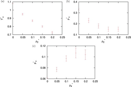
At the end, we checked by Monte Carlo simulations how critical points moves when we add more and more non-polar component into the system. In Figure 10, we are showing how critical point (temperature, pressure and density) of solution depends on the density of second component. Critical temperature decrease almost linearly. Critical pressure shows minima and critical density maxima as function of density of second non-polar component. In this region, PY and HNC do not converge, while SMSA and KH give unphysical correlation functions, meaning wrong results for pressure.

Figure 10. Monte Carlo results for (a) critical temperature, (b) density and (c) pressure as function of ${\rho }_2$ for same size of solute ${\sigma }_{22}$=1.0 as solvent.

6. Conclusions

We have examined the thermodynamics, structure, and phase transitions in two-dimensional mixtures of core-softened fluid with water like properties and non-polar particles using the Monte Carlo computer simulations and the integral equation theories with different closures: PY, HNC, SMSA, and KH. The main conclusion of this work is that, for the system under study, the integral equation theory represents a viable alternative to computer simulations. The IET is faster from the computational point of view than the Monte Carlo simulations; however, it reproduces the structure only qualitatively at some state points. We systematically examined several closures and the results are: the PY and HNC lose convergence at low temperatures. KH can have unphysical solutions at high densities. PY somehow performed best in area of convergence. Overall SMSA has very wide range of convergence and good prediction of thermodynamics. By Monte Carlo simulations, we also determined how the liquid–gas critical point moves with increasing content of non-polar particles.

Acknowledgments

The financial support of the Slovenian Research Agency through Grant P1-0201 as well as to projects J7-1816, J1-1708, N1-0186 and N2-0067 is acknowledged as well as National Institutes for Health RM1 award RM1GM135136.

Disclosure statement

No potential conflict of interest was reported by the author(s).

Additional information

Funding

The financial support of the study was provided by the Slovenian Research Agency through Grant P1-0201 as well as to projects J7-1816, J1-1708, N1-0186 and N2-0067 as well as by the National Institutes for Health RM1 award RM1GM135136.

References

- Barker JA, Henderson D, Abraham FF. Phase diagram of the two-dimensional Lennard-Jones system: evidence for first-order transitions. Phys A. 1981;106:226–238.
- Phillips JM, Bruch LW, Murphy RD. The two-dimensional Lennard-Jones system: sublimation, vaporization, and melting. J Chem Phys. 1981;75:5097–5109.
- Scalise OH, Zarragoicoechea GJ, Gonzalez LE, et al. Phase equilibria of the two-dimensional Lennard-Jones fluid: reference systems and perturbation theories. Mol Phys. 1998;93:751–755.
- Scalise OH. Vapour-liquid coexistence in a quasi two-dimensional hard dipolar fluid. Phys Chem Liq. 1998;36:179–185.
- Zarragoicoechea GJ. A model phospholipid monolayer: a computer simulation study. Mol Phys. 1999;96:1109–1113.
- Scalise OH, Zarragoicoechea GJ, Silbert M. Critical behaviour of two-dimensional Lennard-Jones fluid mixtures: a mean field study. Phys Chem Chem Phys. 1999;1:4241–4244.
- Scalise OH. Type I gas-liquid equilibria of a two-dimensional Lennard-Jones binary mixtureFluid Phase Equilib. 2001;182:59–64.
- Birdi KS. Lipid and bipolymer monolayers at liquid interfaces. New York: Plenum Press; 1989.
- Toxvaerd S. The mobile-layer model for adsorption. Mol Phys. 1975;29:373–379.
- Smit B, Frenkel D. Vapor-liquid equilibria of the two-dimensional Lennard-Jones fluid(s). J Chem Phys. 1991;94:5663–5668.
- Toxvaerd S. Melting in a two-dimensional Lennard-Jones system. J Chem Phys. 1978;69:4750–4752.
- Abraham FF. Melting in two dimensions is first order: an isothermal-isobaric Monte Carlo study. Phys Rev Lett. 1980;44:463–466.
- Puntam FA, Fort T. Physical adsorption of patchwise heterogeneous surfaces. I. Heterogeneity, two-dimensional phase transitions, and spreading pressure of the krypton-graphitized carbon black system near 100.deg.K. J Phys Chem. 1975;79:459–467.
- Thomy A, Duval X. Adsorption de molecules simples sur graphite. J Chim Phys. 1970;67:1101–1110.
- Silverstein KAT, Haymet ADJ, Dill KA. A simple model of water and the hydrophobic effect. J Am Chem Soc. 1998;120:3166–3175.
- Southall NT, Dill KA. A view of the hydrophobic effect. J Phys Chem B. 2002;106:521–533.
- Urbic T, Vlachy V, Kalyuzhnyi Yu. V, et al. A two-dimensional model of water: theory and computer simulations. J Chem Phys. 2000;112:2843–2848.
- Urbic T, Vlachy V, Kalyuzhnyi Yu. V, et al. A two-dimensional model of water: solvation of nonpolar solutes. J Chem Phys. 2002;116:723–729.
- Urbic T, Vlachy V, Kalyuzhnyi Yu.V, et al. Orientation-dependent integral equation theory for a two-dimensional model of water. J Chem Phys. 2003;118:5516–5525.
- Ben–Naim AJ. Statistical mechanics of “Waterlike” particles in two dimensions. I. physical model and application of the Percus–Yevick equation. Chem Phys. 1971;54:3682.
- Eisenberg D, Kauzmann W. The structure and properties of water. Oxford: Oxford University Press; 1969.
- Franks F. Water: a comprehensive treatise. New York: Plenum; 19721780.
- Stillinger FH. Water Revisited. Sci. 1980;209:451–457.
- Sharma R, Chakraborty SN, Chakravarty C. Entropy, diffusivity, and structural order in liquids with waterlike anomalies. J Chem Phys. 2006;125:204501.
- Poole PH, Hemmati M, Angell CA. Comparison of thermodynamic properties of simulated liquid silica and water. Phys Rev Lett. 1997;79:2281–2284.
- Shell MS, Debenedetti PG, Panagiotopoulos AZ. Generalization of the Wang-Landau method for off-lattice simulations. Phys Rev E. 2002;66:056703.
- Hemmer PC, Stell G. Fluids with several phase transitions. Phys Rev Lett. 1970;24:1284–1287.
- de Oliveira AB, Netz PA, Barbosa MC. Which mechanism underlies the water-like anomalies in core-softened potentials?. Eur Phys J B. 2008;64:481–486.
- Sastry S, Angell CA. Liquid-liquid phase transition in supercooled silicon. Nat Mater. 2003;2:739–743.
- Angell CA, Bressel RD, Hemmati M, et al. Water and its anomalies in perspective: tetrahedral liquids with and without liquid–liquid phase transitions. Phys Chem Chem Phys. 2000;2:1559.
- Mon KK, Ashcroft NW, Chester GV. Core polarization and the structure of simple metals. Phys Rev B. 1979;19:5103–5122.
- Levesque D, Weis JJ. Structure factor of a system with shouldered hard sphere potential. Phys Lett A. 1977;60:473–474.
- Cummings PT, Stell G. Mean spherical approximation for a model liquid metal potential. Mol Phys. 1981;43:1267–1291.
- Voronel A, Paperno I, Rabinovich S, et al. New critical point at the vicinity of the freezing temperature of K2Cs. Phys Rev Lett. 1983;50:247.
- Velasco E, Mederos L, Navascues G, et al. Complex phase behavior induced by repulsive interactions. Phys Rev Lett. 2000;85:122.
- Poole PH, Sciortino F, Essmann U, et al. Phase behaviour of metastable water. Nature. 1992;360:324–328.
- Buldyrev SV, Franzese G, Giovambattista N, et al. Models for a liquid-liquid phase transition. Phys A. 2002;304:23–42.
- Urbic T. Liquid-liquid phase transition in a two-dimensional system with anomalous liquid properties. Phys Rev E. 2013;88:062303.
- Almudallal AM, Buldyrev SV, Saika-Voivod I. Phase diagram of a two-dimensional system with anomalous liquid properties. J Chem Phys. 2012;137:034507.
- Franzese G, Malescio G, Skibinsky A, et al. Generic mechanism for generating a liquid-liquid phase transition. Nature. 2001;409:692–695.
- Bizjak A, Urbic T, Vlachy V, et al. The three–dimensional “Mercedes Benz” model of water. Acta Chim Slov. 2007;54:532.
- Bizjak A, Urbic T, Vlachy V, et al. Theory for the three-dimensional Mercedes-Benz model of water. J Chem Phys. 2009;131:194504.
- Sadr-Lahijany MR, Scala A, Buldyrev SV, et al. Liquid-state anomalies and the Stell-Hemmer core-softened potential. Phys Rev Lett. 1998;81:4895–4898.
- Sadr-Lahijany MR, Scala A, Buldyrev SV, et al. Waterlike anomalies for core-softened models of fluids: one dimension. Phys Rev E. 1999;60:6714–6721.
- Scala A, Reza Sadr-Lahijany M, Giovambattista N, et al. Waterlike anomalies for core-softened models of fluids: two-dimensional systems. Phys Rev E. 2001;63:041202.
- Frenkel D, Smit B. Molecular simulation: from algorithms to applications. New York: Academic Press; 2000.
- Ornstein LS, Zernike F. Accidental deviations of density and opalescence at the critical point of a single substance. Proc Akad Sci (Amsterdam). 1914;17:793.
- Morita T, Hiroike K. A new approach to the theory of classical fluids. I: Prog Theor Phys. 1960;23:829.
- Percus JK, Yevick GJ. Analysis of classical statistical mechanics by means of collective coordinates. Phys Rev. 1958;110:1–13.
- Percus JK. Approximation methods in classical statistical mechanics. Phys Rev Lett. 1962;8:462–463.
- Kovalenko A, Hirata F. Self-consistent description of a metal-water interface by the Kohn-Sham density functional theory and the three-dimensional reference interaction site model. J Chem Phys. 1999;110:10095–10112.
- Rick SW, Haymet ADJ. Density functional theory for the freezing of Lennard-Jones binary mixtures. J Chem Phys. 1989;90:1188–1199.
- Talman JD. Numerical Fourier and Bessel transforms in logarithmic variables. J Comput Phys. 1978;29:35–48.
- Urbic T, Dias CL. Properties of the Lennard-Jones dimeric fluid in two dimensions: an integral equation study. J Chem Phys. 2014;140:094703.
- Urbic T. Properties of the two-dimensional heterogeneous Lennard-Jones dimers: an integral equation study. J Chem Phys. 2016;145:194503.