RUPTURA: simulation code for breakthrough, ideal adsorption solution theory computations, and fitting of isotherm models

ABSTRACT

We present the RUPTURA code (https://github.com/iraspa/ruptura) as a free and open-source software package (MIT license) for (1) the simulation of gas adsorption breakthrough curves, (2) mixture prediction using methods like the Ideal Adsorption Solution Theory (IAST), segregated-IAST and explicit isotherm models, and (3) fitting of isotherm models on computed or measured adsorption isotherm data. The combination with the RASPA software enables computation of breakthrough curves directly from adsorption simulations in the grand-canonical ensemble. RUPTURA and RASPA have similar input styles. IAST is implemented near machine precision but we also provide several explicit mixture prediction methods that are non-iterative and potentially faster than IAST. The code supports a wide variety of isotherm models like Langmuir, Anti-Langmuir, BET, Henry, Freundlich, Sips, Langmuir-Freundlich, Redlich-Peterson, Toth, Unilan, O'Brian & Myers, Asymptotic Temkin, and Bingel & Walton. The isotherm model parameters can easily be obtained by the fitting module. Breakthrough plots and animations of the column properties are automatically generated. In addition to highlighting the code, we also review all the developed techniques from literature for mixture prediction, breakthrough simulations, and isotherm model fitting, and provide a tutorial discussing the workflows.

KEYWORDS:

• Breakthrough
• fixed-bed
• IAST
• isotherm model
• RUPTURA

Nomenclature

T	=	absolute temperature, K
R	=	universal gas constant, 8.314464919 J mol${}^{-1}$ K${}^{-1}$
S	=	entropy, J K${}^{-1}$
V	=	volume, m${}^3$
L	=	length of packed bed adsorber, m
m	=	mass, kg
N	=	number of molecules, –
$N_{{}_C}$	=	number of components, –
n	=	number of moles, –
p, $p_{{}_T}$	=	total pressure in the bulk fluid phase, Pa
f	=	fugacity, Pa
ϕ	=	fugacity coefficient, –
${\mu }_i$	=	chemical potential of component i, J mol${}^{-1}$
$q_i$	=	adsorbed loading of species i, mol (kg framework)${}^{-1}$
${\overline{q}}_i$	=	average molar loading of species i, mol (kg framework)${}^{-1}$
$q_i^{\ast }$	=	adsorbed loading of pure component i evaluated at the mixture T and Ω, mol (kg framework)${}^{-1}$
$q_{{}_T}$	=	total loading of the mixture, mol (kg framework)${}^{-1}$
$q\left(f\right)$	=	absolute loading of the adsorbed phase as a function of fugacity, mol (kg framework)${}^{-1}$
$q\left(p\right)$	=	absolute loading of the adsorbed phase as a function of pressure, mol (kg framework)${}^{-1}$
$q^{\mathrm{s}\mathrm{a}\mathrm{t}}$	=	saturation loading, mol (kg framework)${}^{-1}$
$q_{\mathrm{e}\mathrm{q}}$	=	equilibrium loading, mol (kg framework)${}^{-1}$
b	=	equilibrium constant, Pa${}^{-1}$
θ	=	fractional loading, -
$x_i$	=	mole fraction of species i in the adsorbed phase, –
$y_i$	=	mole fraction of component i in the bulk fluid phase, –
t	=	time, s
v	=	interstitial gas velocity entering the packed bed, m s${}^{-1}$
${ϵ}_{{}_B}$	=	packed bed void fraction, –
$\mathcal{D}$	=	axial dispersion coefficient, m${}^2$ s${}^{-1}$
$D_m$	=	molecular diffusion coefficient, m${}^2$ s${}^{-1}$
$D_{{}_K}$	=	Knudsen diffusion coefficient, m${}^2$ s${}^{-1}$
$D_{{}_S}$	=	surface diffusion coefficient, m${}^2$ s${}^{-1}$
$D_{{}_{MS}}$	=	Maxwell-Stefan diffusion coefficient, m${}^2$ s${}^{-1}$
$D_{{}_F}$	=	Fick diffusion coefficient, m${}^2$ s${}^{-1}$
k	=	mass transfer coefficient, s${}^{-1}$
${\rho }_{{}_B}$	=	bed density, kg m${}^{-3}$ particle density, kg m${}^{-3}$
${\rho }_f$	=	fluid phase density, kg m${}^{-3}$
Ω	=	grand potential $(\mathrm{\Omega }=U-TS-\sum _i{\mu }_i{N}_i)$, J (kg framework)${}^{-1}$
ψ	=	reduced grand potential $(\psi =-\mathrm{\Omega }/(RT\left)\right)$, mol (kg framework)${}^{-1}$
Γ	=	thermodynamic correction factor, -
$r_p$	=	particle size, m
GCMC	=	Grand-Canonical Monte Carlo
PSA	=	Pressure swing adsorption
TSA	=	Temperature swing adsorption
SSP-RK	=	Strong-Stability Preserving Runge-Kutta

Subscripts
i	=	refers to component i
T	=	refers to total mixture or pressure
${}^{\ast }$	=	indicates a property of the pure component evaluated at the mixture T and Ω

1. Introduction

The separation of mixtures are of extreme importance to chemists and chemical engineers [1]. Adsorption based methods are often implemented for the separation of industrial processes such as separation of hydrocarbons [2], ${\mathrm{C}\mathrm{O}}_2$ capture [3], water purification [4], refrigeration [5], etc. Adsorptive separation processes are divided into two broad categories: (a) continuous flow systems and (b) cyclic batch systems [6]. In a continuous flow system, the fluid phase passes through a fixed bed of solid adsorbents. The capacity of the adsorbents depends on the fluid phase velocity and residence time. To maintain the counter-current contact, the adsorbent must be circulated continuously or the circulation should be mimicked through clever semi-continuous design, e.g. by switching process streams [6]. Such requirements lead to a complex design of the separation system and reduced operational flexibility [6]. An example of such a system is the Simulated Moving Bed (SMB) which is widely used for chromatographic applications [7]. Moving bed systems are designed to regenerate adsorbents by another bed by displacement and this is not a common large-scale industrial adsorption setup. In cyclic batch systems, the bed is alternately saturated and regenerated [6]. Based on the method of regenerating the adsorbent, the cyclic systems can be categorised into: (a) Pressure Swing Adsorption (PSA) and (b) Temperature Swing Adsorption (TSA) [8]. In TSA, the adsorber column is regenerated by heating the bed using a hot stream of non-adsorbing gas. This operation is performed at a temperature at which the adsorbed species desorb from the bed and are carried away along with the stream of hot gas. TSA has been widely used for gas drying and volatile organic compound recovery [8]. In PSA, desorption is achieved by lowering the pressure of the column at a constant temperature which is followed by purging of a non-adsorbing stream of gas to remove the desorbed species [6]. Vacuum Pressure Swing Adsorption (VPSA) is a kind of PSA which is used for hydrogen purification, ${\mathrm{C}\mathrm{O}}_2$ capture, and air separation [8].

PSA is a non-cryogenic gas separation technology that achieves very high purity [9]. Pressure-swing adsorbers are operated in cyclic steady-state consisting of a minimum of two fixed beds with adsorbent, which continuously cycle through four dynamic process steps (Skarstrom cycle [10]): pressurisation, adsorption, blow-down, and desorption. The use of more adsorbent columns improves the outlet gas purity and recovery rate because of the possibility of accommodating more pressure equalisation steps in each PSA cycle [11–13]. Pressure equalisation is a process where gas leaving the first column being depressurised is used to partially pressurise the second adsorbent column [13]. Apart from improving the recovery and purity, this process also reduces the energy consumption. The frequency of regeneration is high in case of PSA adsorption systems [6] and it does not have much impact on the adsorbent structures. These systems are designed based on short cycles [6] (ca. seconds to minutes). The frequency of regeneration is a crucial factor in designing TSA-based systems. This is because, frequent thermal regeneration processes can adversely affect the adsorbent structure [6]. Therefore, TSA units are typically designed for longer cycles [6] (ca. hours to days) of operation.

Important factors that determine the economics of PSA units are [14]: (1) high selectivity for the adsorption of one component over the other components present in the gas mixture, (2) high working (adsorption) capacity between the conditions of regeneration and adsorption, (3) mild conditions for regeneration (usually induced by pressure or temperature swings), (4) high stability and resistance against impurities and moisture, and (5) fast adsorption kinetics. These factors most often exclude each other, and chemists and materials scientists attempt to find and rationalise the ‘sweet spot’ for designing adsorbents [14]. In particular, in addition to selectivity, working capacity and recyclability (including the kinetics and energy of regeneration) are also key performance parameters [15]. The working capacity is the difference in loading of the preferentially adsorbed component at the adsorption pressure minus the loading at the purge pressure [16]. The adsorptive delivery should be maximised considering the entire adsorption-desorption cycle [17]. Based on this, an optimal enthalpy of adsorption change can be estimated. Experimental screening of potential adsorbent materials for use in PSA services is time consuming. Therefore, computational screening of possible adsorbent materials for their performance factors is crucial.

Adsorption processes in fixed-bed columns are influenced by first order factors (adsorption equilibrium isotherms) and second order factors (kinetics of intra/inter-particle mass/heat transfer, film/heat mass transfer, dispersion, nature of fluid flow, wall heat transfer) [6,19,20]. The performance of adsorbents in fixed-bed adsorbers can be evaluated by performing ‘breakthrough’ simulations. A schematic diagram of fixed-bed adsorber is shown in Figure 1. A fixed bed packed with particles containing porous materials is pressurised and purged with a carrier gas. A fluid is added to the carrier gas and the change of the component concentrations along the column and at the outlet of the fixed bed are recorded. Depending upon process objectives, a fixed-bed operation may be divided into three types: saturation adsorption, elution, and chromatography [20]. For saturation adsorption, a feed solution is passed through a column packed with adsorbents for the purpose of removal of the preferentially adsorbed component. This process continues until the adsorbents become sufficiently saturated, and the solute removal rate diminishes to the extent that termination of operation becomes necessary. Elution (desorption) is a process in which a solvent is passed through a column of adsorbents saturated with solutes. For chromatographic applications, a pulse of the mixture is introduced into a carrier fluid flowing through a column packed with adsorbents [20]. Pulse breakthrough is affected by both adsorption and desorption.

Figure 1. (Colour online) Schematic diagram of fixed-bed adsorber. A peristaltic compressor/pump is used to maintain a constant flow rate. In most gas-phase adsorbers, the gas enters from the top and flows down through the bed, while in a typical liquid system the column fills upwards [18]. The outlet of the bed is connected to a sample collector.

Despite the importance of breakthrough simulations, there is a lack of open-source software to predict breakthrough curves in fixed-bed adsorbers. In this article, we present such a software package named ‘RUPTURA’. The code is available under the MIT license and downloadable from github (https://www.github.com/iraspa/ruptura). Mixture prediction and breakthrough simulations rely on isotherm models that can be obtained by fitting isotherm data. RASPA [21,22] is a software package for simulating adsorption of molecules in nanoporous materials. The combination with RASPA enables computation of breakthrough curves directly from the pure component adsorption simulations in the grand-canonical ensemble. RUPTURA and RASPA have similar input styles. RUPTURA contains three modules of workflow encountered in this field: (1) the computation of step and pulse breakthrough, (2) the prediction of mixture adsorption (used in the breakthrough equations) based on pure component isotherms, and (3) the fitting of isotherm models on raw (computed or measured) isotherm data. Many isotherm models have been published in the literature [20,23–27]. We included isotherm models like Langmuir, BET, Henry, Freundlich, Sips, Langmuir-Freundlich, Redlich-Peterson, Toth, Unilan, O'Brien & Myers and Asymptotic Temkin, as well as their multi-site versions or combinations of those. The implemented mixture prediction methods are: Ideal Adsorption Solution Theory (IAST) [28], segregated IAST [29], Explicit Isotherm (EI) model [30] and Segregated Explicit Isotherm (SIAST) model [31]. IAST is computed fast and near machine precision. The breakthrough simulations include axial dispersion and the Linear Driving Force (LDF) model for mass-transfer [32], and use a numerically stable method called Strong-Stability Preserving Runge-Kutta (SSP-RK) for the numerical integration [33–37].

We foresee our code being used in (industrial) research for screening adsorbents for separation processes based on PSA, and TSA but also for teaching in chemistry and chemical engineering classes. Hence, in this article we combine the presentation of our code with a review of the underlying theory and methodologies, and a tutorial. The teaching aspect is also the reason why the numerical schemes and fitting procedure are described in detail. The tutorial aspect also implied that we aim to make our code as easy to use as possible, and that the generation of breakthrough pictures and movies is automatic. It is also vital that researchers and students would be able to play around with examples that run in the order of minutes. This is interactive enough to investigate the effect of adsorption, axial dispersion, mass-transfer coefficients, column void fraction, flow velocity, and column length on the breakthrough and separation efficiency. To achieve even higher computational speed, we included isotherm models of explicit nature (EI and SEI) that, although limited to Langmuir behaviour, work for any number of components [30].

Our article is organised as follows. We begin by explaining models for pure component isotherms (Section 2) and discuss the methodology to predict mixture results from pure component isotherm in Section 3. Such methodologies include IAST and we detail our implementation and validate it by comparing it to previous work. Section 4 contains the theory on breakthrough simulations and our detailed numerical implementation. In Section 5, we focus on our genetic-algorithm implementation of isotherm fitting. We close our article with a description of the installation instructions (Section 6), the input format and options (Section 7), a tutorial (Section 8), and a troubleshooting section (Section 9). Our main findings are summarised in Section 10.

2. Isotherm models

2.1. Introduction

Adsorption is a surface process that involves the transfer of a molecule from a bulk fluid to a solid surface. Physical adsorption is caused by Van der Waals forces (includes dipole–dipole, dipole-induced dipole, London forces, and possibly hydrogen bonding) [38,39]. An adsorbate is a molecule adsorbed on the surface of the solid material, and the solid material is referred to as the adsorbent. An adsorption process is the addition of adsorbate to the adsorbent by increasing the adsorptive pressure, while desorption is the removal of adsorbate from the adsorbent by decreasing the adsorptive pressure or/and increasing the temperature [39,40]. Experimental adsorption data are routinely reported as net or excess amounts adsorbed, while simulations such as molecular simulations measure absolute adsorption. The excess adsorbed amount refers to the difference between the actual (absolute) amount adsorbed and the amount that would be present in the same volume at the density of the fluid in the bulk phase [41,42]. The net adsorbed amount has a reference state that does not require the knowledge of the adsorbent volume, and the solid and adsorbed phase are being treated as an entity [43]. Statistical thermodynamic theories and molecular simulations of adsorption of gases on porous solids are formulated in the language of absolute thermodynamic variables [44].

The fundamental concept in adsorption science is the adsorption isotherm, i.e. the equilibrium relation between the quantity of the adsorbed material and the pressure or concentration in the bulk fluid phase at constant temperature [40]. Mathematically, we can describe absolute adsorption of an adsorbate on an adsorbent with a smooth, continuous function $q\left(c_i\right)$ that represents the dependency of the adsorbed phase concentration $q_i$ of a component i on the fluid phase concentrations $c_i$ (1) $q_i=q(c_1,c_2,\dots ,c_{N_C})\mathrm{a}\mathrm{t}\mathrm{c}\mathrm{o}\mathrm{n}\mathrm{s}\mathrm{t}\mathrm{a}\mathrm{n}\mathrm{t}T$(1) Common units for the loading q include mol/(kg framework) and mg/(mg framework) with $q\ge 0$. For a single component system, we generally have $\mathrm{d}q/\mathrm{d}p\ge 0$. The adsorption of a component depends not only on the concentration of this component, $c_i$, but also on the equilibrium concentrations of all other components. Likewise, we could describe adsorption from an ideal gas phase by substituting the fluid phase concentrations by partial pressures in the gas phase (2) $q_i=q(p_1,p_2,\dots ,p_{N_{{}_C}})\mathrm{a}\mathrm{t}\mathrm{c}\mathrm{o}\mathrm{n}\mathrm{s}\mathrm{t}\mathrm{a}\mathrm{n}\mathrm{t}T$(2) The adsorption equilibrium of a single adsorbate can be described by the adsorption isotherm (3) $q=q\left(p\right)\mathrm{a}\mathrm{t}\mathrm{c}\mathrm{o}\mathrm{n}\mathrm{s}\mathrm{t}\mathrm{a}\mathrm{n}\mathrm{t}T$(3) In general, an increase in the temperature will lead to a decreased amount adsorbed at a given pressure. In case the isotherm model has a well-defined saturation loading $q^{\mathrm{s}\mathrm{a}\mathrm{t}}$, a fractional loading θ can be defined (4) $\theta \left(p\right)=\frac{q\left(p\right)}{q^{\mathrm{s}\mathrm{a}\mathrm{t}}}$(4) The Henry coefficient $H_K$ for adsorption is defined as (5) $H_K=\underset{p\to 0}{lim}\frac{q\left(p\right)}{p}=\underset{p\to 0}{lim}\frac{\mathrm{d}q}{\mathrm{d}p}$(5) The Henry coefficient is the slope of the isotherm at very low pressure. In this infinite dilution regime, there are no adsorbate-adsorbate interactions, and adsorption is linearly related to the affinity of the adsorbate. Note that the Henry coefficient depends on temperature.

2.2. Isotherm models

Isotherm models are well described in various resources [20,23–27]. New isotherm models continue to be developed. For example, the new Bingel-Walton isotherm model allows for a continuous, mathematical description of general type V isotherms, which appear in novel flexible MOFs or many water adsorption cases [45]. We will describe some of the isotherm models that are implemented in RUPTURA. The mathematical description for the functional form, the Henry coefficient, the saturation value, and the order of input of the arguments in the code are summarised in Table 1. The derived formulas for the inverse of the isotherm are listed in Table 2.

Table 1. Isotherm models, Henry and saturation regime, and the order of input of the arguments in RUPTURA.

Model	Equation	Henry	saturation	$b_0$	$b_1$	$b_2$
Langmuir [46]	$q\left(p\right)=q^{\mathrm{s}\mathrm{a}\mathrm{t}}\frac{bp}{1+bp}$	$b{q}^{\mathrm{s}\mathrm{a}\mathrm{t}}$	$q^{\mathrm{s}\mathrm{a}\mathrm{t}}$	$q^{\mathrm{s}\mathrm{a}\mathrm{t}}$	b
n-site Langmuir	$q\left(p\right)=\sum _i{q}_i^{\mathrm{s}\mathrm{a}\mathrm{t}}\frac{b_{i}p}{1+b_{i}p}$	$\sum _i{b}_i{q}^{\mathrm{s}\mathrm{a}\mathrm{t}}$	$\sum _i{q}_i^{\mathrm{s}\mathrm{a}\mathrm{t}}$	$q^{\mathrm{s}\mathrm{a}\mathrm{t}}$	b
BET [47]	$q\left(p/p^0\right)=q^{\mathrm{s}\mathrm{a}\mathrm{t}}\frac{b\left(p/p^0\right)}{(1-c(p/p^0\left)\right)(1-c+b(p/p^0\left)\right)}$	$\frac{b{q}^{\mathrm{s}\mathrm{a}\mathrm{t}}}{1-c}$	$\frac{b{q}^{\mathrm{s}\mathrm{a}\mathrm{t}}}{(1-c)(1-c+b)}$	$q^{\mathrm{s}\mathrm{a}\mathrm{t}}$	b	c
Anti-Langmuir [24]	$q\left(p\right)=\frac{ap}{1-bp}$	a	✗	a	b
Henry	$q\left(p\right)=ap$	a	✗	a
Freundlich [48]	$q\left(p\right)=a{p}^{1/\nu }$	✗	✗	a	ν
Sips [49]	$q\left(p\right)=q^{\mathrm{s}\mathrm{a}\mathrm{t}}\frac{(bp{)}^{1/\nu }}{1+(bp{)}^{1/\nu }}$	✗	$q^{\mathrm{s}\mathrm{a}\mathrm{t}}$	$q^{\mathrm{s}\mathrm{a}\mathrm{t}}$	b	ν
n-site Sips	$q\left(p\right)=\sum _i{q}_i^{\mathrm{s}\mathrm{a}\mathrm{t}}\frac{(b_{i}p{)}^{1/{\nu }_i}}{1+(b_{i}p{)}^{1/{\nu }_i}}$	✗	$\sum _i{q}_i^{\mathrm{s}\mathrm{a}\mathrm{t}}$	$q^{\mathrm{s}\mathrm{a}\mathrm{t}}$	b	ν
Langmuir-Freundlich [50]	$q\left(p\right)=q^{\mathrm{s}\mathrm{a}\mathrm{t}}\frac{b{p}^{\nu }}{1+b{p}^{\nu }}$	✗	$q^{\mathrm{s}\mathrm{a}\mathrm{t}}$	$q^{\mathrm{s}\mathrm{a}\mathrm{t}}$	b	ν
n-site Langmuir-Freundlich	$q\left(p\right)=\sum _i{q}_i^{\mathrm{s}\mathrm{a}\mathrm{t}}\frac{b_i{p}_i^{\nu }}{1+b_i{p}_i^{\nu }}$	✗	$\sum _i{q}_i^{\mathrm{s}\mathrm{a}\mathrm{t}}$	$q^{\mathrm{s}\mathrm{a}\mathrm{t}}$	b	ν
Redlich-Peterson [51]	$q\left(p\right)=\frac{ap}{1+b{p}^{\nu }}$	a	✗	a	b	ν
Toth [52–54]	$q\left(p\right)=q^{\mathrm{s}\mathrm{a}\mathrm{t}}\frac{bp}{[1+(bp{)}^{\nu }{]}^{1/\nu }}$	$b{q}^{\mathrm{s}\mathrm{a}\mathrm{t}}$	$q^{\mathrm{s}\mathrm{a}\mathrm{t}}$	$q^{\mathrm{s}\mathrm{a}\mathrm{t}}$	b	ν
Unilan	$q\left(p\right)=q^{\mathrm{s}\mathrm{a}\mathrm{t}}\frac{1}{2\eta }\ln \left[\frac{1+b{e}^{\eta }p}{1+b{e}^{-\eta }p}\right]$	$b{q}^{\mathrm{s}\mathrm{a}\mathrm{t}}$	$q^{\mathrm{s}\mathrm{a}\mathrm{t}}$	$q^{\mathrm{s}\mathrm{a}\mathrm{t}}$	b	η
O'Brien & Myers [55]	$q\left(p\right)=q^{\mathrm{s}\mathrm{a}\mathrm{t}}[\frac{bp}{1+bp}+{\sigma }^2\frac{bp(1-bp)}{2(1+bp{)}^3}]$	$q^{\mathrm{s}\mathrm{a}\mathrm{t}}b(1+\frac{{\sigma }^2}{2})$	$q^{\mathrm{s}\mathrm{a}\mathrm{t}}$	$q^{\mathrm{s}\mathrm{a}\mathrm{t}}$	b	σ
Quadratic [56,57]	$q\left(p\right)=q^{\mathrm{s}\mathrm{a}\mathrm{t}}\frac{bp+2c{p}^2}{1+bp+c{p}^2}$	$b{q}^{\mathrm{s}\mathrm{a}\mathrm{t}}$	$2q^{\mathrm{s}\mathrm{a}\mathrm{t}}$	$q^{\mathrm{s}\mathrm{a}\mathrm{t}}$	b	c
Asymptotic Temkin [58,59]	$q\left(p\right)=q^{\mathrm{s}\mathrm{a}\mathrm{t}}\frac{bp}{1+bp}+q^{\mathrm{s}\mathrm{a}\mathrm{t}}\theta {\left(\frac{bp}{1+bp}\right)}^2(\frac{bp}{1+bp}-1)$	$b{q}^{\mathrm{s}\mathrm{a}\mathrm{t}}$	$q^{\mathrm{s}\mathrm{a}\mathrm{t}}$	$q^{\mathrm{s}\mathrm{a}\mathrm{t}}$	b	θ
Bingel & Walton [45]	$q\left(p\right)=q^{\mathrm{s}\mathrm{a}\mathrm{t}}\frac{1-\exp [-(a+b\left)p\right]}{1+\left(b/a\right)\exp [-(a+b\left)p\right]}$	$a{q}^{\mathrm{s}\mathrm{a}\mathrm{t}}$	$q^{\mathrm{s}\mathrm{a}\mathrm{t}}$	$q^{\mathrm{s}\mathrm{a}\mathrm{t}}$	a	b

Table 2. Isotherm models and their inverse.

Model	inverse
Langmuir	$p\left(q\right)=\frac{q}{b(q^{\mathrm{s}\mathrm{a}\mathrm{t}}-q)}$
n-site Langmuir	numerical
BET	$p\left(q\right)=\frac{-b{q}^{\mathrm{s}\mathrm{a}\mathrm{t}}+bq-cq+c^{2}q\pm \sqrt{4bcq(q-cq)+(-b{q}^{\mathrm{s}\mathrm{a}\mathrm{t}}+bq-cq+c^{2}q{)}^2}}{2bcq}$
Anti-Langmuir	$p\left(q\right)=\frac{q}{(a+bq)}$
Henry	$p\left(q\right)=q/a$
Freundlich	$p\left(q\right)={\left(\frac{q}{a}\right)}^{\nu }$
Sips	$p\left(q\right)=\frac{1}{b}{\left(\frac{q}{q^{\mathrm{s}\mathrm{a}\mathrm{t}}-q}\right)}^{\nu }$
n-site Sips	numerical
Langmuir-Freundlich	$p\left(q\right)={\left(\frac{q}{q^{\mathrm{s}\mathrm{a}\mathrm{t}}b-qb}\right)}^{1/\nu }$
n-site Langmuir-Freundlich	numerical
Redlich-Peterson	numerical
Toth	$p\left(q\right)=\frac{q}{(q^{\mathrm{s}\mathrm{a}\mathrm{t}}b-qb){)}^{1/\nu }}$
Unilan	$p\left(q\right)=\frac{e^{\eta }(\exp (\frac{2\eta q}{q^{\mathrm{s}\mathrm{a}\mathrm{t}}})-1)}{b(e^{2\eta }-\exp (\frac{2\eta q}{q^{\mathrm{s}\mathrm{a}\mathrm{t}}}\left)\right)}$
O'Brien & Myers	not shown here
Quadratic	$p\left(q\right)=\frac{-b{q}^{\mathrm{s}\mathrm{a}\mathrm{t}}+bq\pm \sqrt{(b{q}^{\mathrm{s}\mathrm{a}\mathrm{t}}-bq{)}^2+4q(2c{q}^{\mathrm{s}\mathrm{a}\mathrm{t}}-cq)}}{2(2c{q}^{\mathrm{s}\mathrm{a}\mathrm{t}}-cq)}$
Asymptotic Temkin	not shown here
Bingel & Walton [45]	numerical

Notes: The inverse of the O'Brien & Myers and Temkin model are too long to write down here, but can easily be computed symbolically using Mathematica. Note that multi-site combinations will always need to be computed numerically.

2.2.1. Langmuir model

The Langmuir equation is the cornerstone of all theories of adsorption. Langmuir (1918) was the first to propose a coherent theory of adsorption onto a flat surface based on a kinetic viewpoint [46]. The assumptions of the Langmuir model are:

(1)	The surface is homogeneous: all adsorption sites are energetically identical.
(2)	The adsorption is localised: one molecule per adsorption site (monolayer).
(3)	There are no lateral interactions between adsorbed molecules.

These assumptions are often true for chemisorption. Using these assumptions, the Langmuir isotherm can be derived as: (6) $q\left(p\right)=q^{\mathrm{s}\mathrm{a}\mathrm{t}}\frac{bp}{1+bp}{q}^{\mathrm{s}\mathrm{a}\mathrm{t}}\ge 0,b>0$(6) where $q^{\mathrm{s}\mathrm{a}\mathrm{t}}$ is the saturation capacity and b is the coefficient of adsorption representing the affinity of the molecule. In the limit of high pressure, the isotherm will approach $q^{\mathrm{s}\mathrm{a}\mathrm{t}}$. At very low pressures, we obtain Henry's law, with a Henry coefficient of $b{q}^{\mathrm{s}\mathrm{a}\mathrm{t}}$.

The bi-Langmuir suggested by Graham [60] is the simplest model for adsorption onto a non-homogeneous surface [24] (7) $q\left(p\right)=q_1^{\mathrm{s}\mathrm{a}\mathrm{t}}\frac{b_{1}p}{1+b_{1}p}+q_2^{\mathrm{s}\mathrm{a}\mathrm{t}}\frac{b_{2}p}{1+b_{2}p}$(7) in which the subscripts refer to the two adsorption sites. In general, a heterogeneous surface with several distinct types of homogeneous adsorption sites can be modeled with an n-site model: (8) $q\left(p\right)=\sum _{i=1}^n{q}_i^{\mathrm{s}\mathrm{a}\mathrm{t}}\frac{b_{i}p}{1+b_{i}p}$(8) with a saturation value $\sum _i{q}_i^{\mathrm{s}\mathrm{a}\mathrm{t}}$ and Henry coefficient value $\sum _i{b}_i{q}_i^{\mathrm{s}\mathrm{a}\mathrm{t}}$. Multi-site models are required to model isotherms with inflections (‘kinks’). Molecular simulations were able to explain the molecular origins of inflections in isotherms by examining the locations of molecules as a function of pressure [61,62].

2.2.2. Anti-Langmuir model

The anti-Langmuir model describes the behaviour where with increased concentration or pressure, the adsorbed loading increases towards infinity [63]. At very low concentration or pressure, this model obeys Henry's law. The anti-Langmuir isotherm expression reads [24,63]: (9) $q\left(p\right)=\frac{ap}{1-bp}0\le p\le 1/b,b\ge 0$(9) In Equation (9(9) $q\left(p\right)=\frac{ap}{1-bp}0\le p\le 1/b,b\ge 0$(9) ), a represents the Henry coefficient in mol kg${}^{-1}$ Pa${}^{-1}$ and b is the equilibrium constant in Pa${}^{-1}$. The anti-Langmuir model does not have a saturation loading as the maximum loading can increase up to infinity at pressure or concentration equal to 1/b.

2.2.3. Henry model

All isotherms should in principle converge to Henry's law at infinite dilution. In the Henry's regime, the amount adsorbed is proportional to the pressure. The Henry's isotherm model is described by (10) $q\left(p\right)=ap$(10) where a is the energetic constant (Henry constant), and only depends on temperature.

2.2.4. BET model

The Brunauer, Emmett, and Teller (BET) model extends adsorption to multi-layers [47]: (11) $q\left(p\right)=q^{\mathrm{s}\mathrm{a}\mathrm{t}}\frac{b_s\left(p\right)}{(1-b_l\left(p\right))(1-b_l+b_s\left(p\right))}$(11) where $b_s$ and $b_l$ are the equilibrium constants of adsorption on the bare surface and on a layer of previously adsorbed adsorbates, respectively. Similar to the Langmuir model, it is derived from kinetic adsorption-desorption relations. The assumptions made in this model are:

(1)	Each molecule in the first adsorbed layer provides an adsorption site for the second layer, and so on.
(2)	Molecules in the second and subsequent layers are assumed to behave essentially as those in the bulk liquid.

2.2.5. Freundlich model

Boedeker proposed the following empirical isotherm equation [48] (12) $q\left(p\right)=a{p}^{1/\nu }$(12) for the adsorption of polar compounds on polar adsorbents, where the exponent $1/\nu$ is smaller than unity. It has been popularised by Freundlich and therefore known as the Freundlich isotherm. The Freundlich isotherm can be considered a composite of Langmuir isotherms with different b values representing patches of adsorption sites with different adsorption energies [64]. It was shown that summing up a number of Langmuir isotherms leads to Freundlich-type isotherms [65]. The isotherm model can describe adsorption on many heterogeneous surfaces well. However, the model is unable to describe any plateauing trend and also does not have a Henry's regime (in fact, the initial slope is infinite). As a result, some authors have mentioned that this isotherm type is unsuitable for the calculation of the reduced grand potential and other thermodynamic properties [66].

2.2.6. Sips model

Sips proposed an equation similar in form to the Freundlich equation, but it has a finite limit when the pressure is sufficiently high [49]: (13) $q\left(p\right)=q^{\mathrm{s}\mathrm{a}\mathrm{t}}\frac{{\left(bp\right)}^{1/\nu }}{1+{\left(bp\right)}^{1/\nu }}$(13) In this model, the additional parameter ν is a parameter characterising the heterogeneity of the system. The theoretical basis of the equation is described in the book of Do [23]. There also exists a multi-site form (14) $q\left(p\right)=\sum _i{q}_i^{\mathrm{s}\mathrm{a}\mathrm{t}}\frac{{\left(b_{i}p\right)}^{1/{\nu }_i}}{1+{\left(b_{i}p\right)}^{1/{\nu }_i}}$(14) The Sips isotherm does not have the correct limiting behaviour at low pressure, i.e. it does not have a Henry's regime (Equation (5(5) $H_K=\underset{p\to 0}{lim}\frac{q\left(p\right)}{p}=\underset{p\to 0}{lim}\frac{\mathrm{d}q}{\mathrm{d}p}$(5) ) diverges), except when $\nu =1$.

2.2.7. Langmuir-Freundlich model

The Langmuir-Freundlich model is given by [50] (15) $q\left(p\right)=q^{\mathrm{s}\mathrm{a}\mathrm{t}}\frac{b{p}^{\nu }}{1+b{p}^{\nu }}$(15) and has the combined form of Langmuir and Freundlich equations. The constant ν is often interpreted as the heterogeneity factor. Values of unity indicate a material with homogeneous binding sites and the isotherm model reduces to the Langmuir model. There also exists a multi-site form (16) $q\left(p\right)=\sum _i{q}_i^{\mathrm{s}\mathrm{a}\mathrm{t}}\frac{b_i{p}^{{\nu }_i}}{1+b_i{p}^{{\nu }_i}}$(16) The Langmuir-Freundlich isotherm does not have the correct limiting behaviour at low pressure, i.e. it does not have a Henry's regime, except when $\nu =1$.

2.2.8. Redlich-Peterson model

The Redlich-Peterson isotherm is an empirical isotherm mix of the Langmuir and Freundlich isotherms. The numerator is the same as the Langmuir isotherm and has the advantage of possessing a Henry region at infinite dilution [51] (17) $q\left(p\right)=\frac{ap}{1+b{p}^{\nu }}$(17) The parameter a can not be interpreted as the saturation loading, except when $\nu =1$ [64].

2.2.9. Toth model

The previous isotherm models have their limitations. The Freundlich, Sips, and Langmuir-Freundlich equations are not valid at very low pressures, while the Henry, Freundlich, and Redlich-Peterson model do not have a finite saturation value. One of the empirical equations that is popularly used and satisfies the two end limits is the Toth equation [52–54]: (18) $q\left(p\right)=q^{\mathrm{s}\mathrm{a}\mathrm{t}}\frac{bp}{{[1+(bp{)}^{\nu }]}^{1/\nu }}$(18) The Toth equation has been used for fitting data of many adsorbates such as hydrocarbons, carbon oxides, hydrogen sulfide, alcohols on activated carbon, and zeolites [23].

2.2.10. Unilan model

The Unilan model owns its name from UNI, for Uniform distribution and LAN, for Langmuir local model [23]. The Unilan model is described by (19) $q\left(p\right)=q^{\mathrm{s}\mathrm{a}\mathrm{t}}\frac{1}{2\eta }\ln \left[\frac{1+b{e}^{\eta }p}{1+b{e}^{-\eta }p}\right]$(19) η is a measurement of the heterogeneity of the adsorbent. High values indicate a highly heterogeneous system. Being a three-parameter model, also the Unilan equation is very often used to describe many data of hydrocarbons, carbon oxides on activated carbon and zeolites. The Unilan equation has the correct behaviour at low and high pressures. In the limit of $\eta =0$ the Langmuir isotherm is recovered.

2.2.11. O'Brien & Myers

The O'Brien and Myers isotherm model is obtained as a truncation to two terms of a series expansion of the adsorption integral equation in terms of the central moments of the adsorption energy distribution [23,55] (20) $q\left(p\right)=q^{\mathrm{s}\mathrm{a}\mathrm{t}}[\frac{bp}{1+bp}+{\sigma }^2\frac{bp(1-bp)}{2{(1+bp)}^3}]$(20) where σ is a measure of the width of the adsorption energy distribution.

2.2.12. Quadratic model

Statistical thermodynamics suggests that the general form of an isotherm equation should be the ratio of two polynomials of the same degree [57]. The polynomial Langmuir isotherm model, derived from statistical mechanics, reads: (21) $q\left(p\right)=q^{\mathrm{s}\mathrm{a}\mathrm{t}}\frac{bp+c{p}^2+d{p}^3+\cdots }{1+bp+c{p}^2+d{p}^3+\cdots }$(21) In practise, the second order isotherm is often used, called the quadratic isotherm model [56,57] (22) $q\left(p\right)=q^{\mathrm{s}\mathrm{a}\mathrm{t}}\frac{bp+2c{p}^2}{1+bp+c{p}^2}$(22) The loading is convex at low pressures but changes concavity as it saturates, yielding an S-shape, i.e. the isotherm exhibits an inflection point.

2.2.13. Asymptotic approximation to the Temkin model

The Temkin isotherm is derived using a mean-field arguments and asymptotic approximation [58,59] (23) $q\left(p\right)=q^{\mathrm{s}\mathrm{a}\mathrm{t}}\frac{bp}{1+bp}+q^{\mathrm{s}\mathrm{a}\mathrm{t}}\theta {\left(\frac{bp}{1+bp}\right)}^2(\frac{bp}{1+bp}-1)$(23) Here, $q^{\mathrm{s}\mathrm{a}\mathrm{t}}$ and b have the same meaning as in the Langmuir isotherm, and θ describes the strength of adsorbate-adsorbate interactions ($\theta <0$ for attraction).

2.2.14. Bingel & Walton model

The Bingel and Walton isotherm model allows for a continuous, mathematical description of general type V isotherms, which appear in novel flexible MOFs or many water adsorption cases [45]. The model is based on the Bass model of innovation diffusion developed in the late 1960s [67]. This model describes the adoption and diffusion of an invention over time and has been widely used in market sales and technology forecasting. Bingel and Walton applied the Bass model to adsorption, where early-adopters can be seen as the intrinsic high-affinity adsorption sites of the surface. The word-of-mouth contribution of slower innovations refers to adsorption mechanisms that are mainly driven by molecules of the same species that are already adsorbed and thus present in the adsorbed phase. The Bingel-Walton adsorption equation reads [45] (24) $q\left(p\right)=q^{\mathrm{s}\mathrm{a}\mathrm{t}}\frac{1-\exp [-(a+b)p]}{1+\left(b/a\right)\exp [-(a+b)p]}$(24) where a>0 is the intrinsic adsorption affinity between the adsorbate and the adsorbent, and b is the clustering coefficient describing strong adsorbate–adsorbate interactions. The simple model combines the effects of early-adopters and word-of-mouth, resulting in curves that resemble either the type I adsorption isotherm shape or S-shaped curves. The location of the inflection point is $\log \left(b/a\right)/(a+b)$. For small values of a and large values of b the isotherm shape becomes strongly step-wise. In the limit of $b\to 0$ the isotherm becomes an exponential function (25) $q\left(p\right)=q^{\mathrm{s}\mathrm{a}\mathrm{t}}(1-\exp [-ap])$(25) while in the limit of $a\to 0$ the adsorption becomes zero. In the limit of $b\to -a$, the isotherm reduces to the Langmuir model (26) $q\left(p\right)=q^{\mathrm{s}\mathrm{a}\mathrm{t}}\frac{ap}{1+ap}$(26) The model has a Henry coefficient of $a{q}^{\mathrm{s}\mathrm{a}\mathrm{t}}$ and a saturation loading of $q^{\mathrm{s}\mathrm{a}\mathrm{t}}$.

2.3. Reduced grand potential

Thermodynamics is the study of energy and its transformations but more generally tries to establish relationships between basic concepts like internal energy U, entropy S, number of particles N, volume V, temperature T, pressure p, and chemical potential μ to describe the behavior of matter and make predictions. For the mixture vapour-liquid equilibrium, the Gibbs-Duhem equation [68] (27) $S\mathrm{d}T-V\mathrm{d}p+\sum _i{n}_i\mathrm{d}{\mu }_i=0$(27) shows that the independent variables which define the standard states for the components of the mixture are T and p. We can compare the Gibbs-Duhem equation to the differential for a solid material [69] (28) $S\mathrm{d}T+\mathrm{d}\mathrm{\Omega }+\sum _i{n}_i\mathrm{d}{\mu }_i=0$(28) and see that the standard states for mixture adsorption will be determined by T and Ω [69]. The grand potential Ω is the characteristic state function for the grand-canonical ensemble and the unit of Ω is J/(kg framework). At constant temperature, we have (29) $\mathrm{d}\mathrm{\Omega }=-S\mathrm{d}T-\sum _i{n}_i\mathrm{d}{\mu }_i=-\sum _i{n}_i\mathrm{d}{\mu }_i$(29) which is the ‘Gibbs adsorption’ equation. Replacing chemical potential ${\mu }_i$ by the fugacity $f_i$ (30) $\mathrm{d}\mathrm{\Omega }=-RT\sum _i{n}_i\mathrm{d}\ln \left[\frac{f_i}{f_0}\right]$(30) where $f_0$ is a reference fugacity to make the argument of the logarithm dimensionless. Replacing fugacity by pressure and integrating for pure-component adsorption from the unadsorbed state at zero pressure, we obtain the grand potential Ω [6,44,70,71] (31) ${\mathrm{\Omega }}_i=-RT{\int }_0^{p_i^{\ast }}{q}_i^{\ast }\left(p\right)\mathrm{d}\ln \left(p\right)\mathrm{o}\mathrm{r}{\mathrm{\Omega }}_i=-RT{\int }_0^{p_i^{\ast }}\frac{q_i^{\ast }\left(p\right)}{p}\mathrm{d}p$(31) where $q_i^{\ast }\left(p\right)$ is the loading of pure component i given as a function of the pressure. Physically, the grand potential is the free energy change associated with isothermal immersion of fresh adsorbent in the bulk fluid. The absolute value of the grand potential is the minimum isothermal work necessary to clean the adsorbent [72]. In calculations, it is convenient to introduce a reduced grand potential ψ [69]: (32) $\psi \left(p_i^{\ast }\right)\equiv -\frac{{\mathrm{\Omega }}_i}{RT}={\int }_0^{p^{\ast }}\frac{q_i^{\ast }\left(p\right)}{p}\mathrm{d}p$(32) The reduced grand potential has units of mol/kg. The integration limit $p_i^{\ast }$ is a property of the pure component property, i.e. it is the pressure at a given reduced grand potential. This quantity is known as the sorption pressure (in analogy to the saturation pressure in vapour-liquid equilibrium) and also as the hypothetical pressure. Importantly, the reduced grand potential is defined in terms of absolute adsorption and can be computed from the adsorption isotherm. In Tables 3 and 4 we list the derived expressions for the reduced grand potential and the sorption pressure (the inverse of the reduced grand potential), respectively, for the various isotherm models.

Table 3. Reduced grand potential for isotherm models.

Model	reduced grand potential $\psi \left(p\right)$
Langmuir [23]	$\psi \left(p\right)=q^{\mathrm{s}\mathrm{a}\mathrm{t}}\ln [1+bp]$
n-site Langmuir [23]	$\psi \left(p\right)=\sum _i{q}_i^{\mathrm{s}\mathrm{a}\mathrm{t}}\ln [1+b_{i}p]$
BET [63]	$\psi \left(p\right)=q^{\mathrm{s}\mathrm{a}\mathrm{t}}\ln \left[\frac{1+bp-cp}{1-cp}\right]$
Anti-Langmuir [24]	$\psi \left(p\right)=-\frac{a}{b}\ln [1-bp]$
Henry	$\psi \left(p\right)=ap$
Freundlich [23]	$\psi \left(p\right)=a\nu p^{1/\nu }$
Sips [23]	$\psi \left(p\right)=q^{\mathrm{s}\mathrm{a}\mathrm{t}}\nu \ln [1+(bp{)}^{1/\nu }]$
n-site Sips	$\psi \left(p\right)=\sum _i{q}_i^{\mathrm{s}\mathrm{a}\mathrm{t}}\nu \ln [1+(b_{i}p{)}^{1/{\nu }_i}]$
Langmuir-Freundlich [73]	$\psi \left(p\right)=\frac{q^{\mathrm{s}\mathrm{a}\mathrm{t}}}{\nu }\ln [1+b{p}^{\nu }]$
n-site Langmuir-Freundlich	$\psi \left(p\right)=\sum _i\frac{q_i^{\mathrm{s}\mathrm{a}\mathrm{t}}}{{\nu }_i}\ln [1+b_i{p}^{{\nu }_i}]$
Redlich-Peterson [74,75]	$\begin{array}{rl}\psi \left(p\right)& =ap{}_2{F}_1(1,1/\nu ,1+1/\nu ,-b{p}^{\nu })\\ & (b{p}^{\nu }<1)\\ & =\frac{a}{\nu b^{1/\nu }}[\frac{\pi }{\sin \left(\pi /\nu \right)}+{\displaystyle \sum _{k=1}^{\mathrm{\infty }}(-1{)}^k\frac{(\frac{1}{b{p}^{\nu }}{)}^{k-1/\nu }}{k-1/\nu }}]\\ & (b{p}^{\nu }>1)\end{array}$
Toth [73,76]	$\begin{array}{rl}\psi \left(p\right)& =q^{\mathrm{s}\mathrm{a}\mathrm{t}}bq{}_2{F}_1(1/\nu ,1/\nu ,1+1/\nu ,-(pb{)}^{\nu })\\ & (b{p}^{\nu }<1)\\ & =q^{\mathrm{s}\mathrm{a}\mathrm{t}}(\theta -\frac{\theta }{\nu }\ln [1-{\theta }^{\nu }]-{\displaystyle \sum _{k=1}^{\mathrm{\infty }}\frac{{\theta }^{k\nu +1}}{k\nu [k\nu +1]}})\end{array}$
Unilan [73]	$\psi \left(p\right)=q^{\mathrm{s}\mathrm{a}\mathrm{t}}\frac{1}{2\eta }\left({\mathrm{L}\mathrm{i}}_2\right(-b{e}^{-\eta }p)-{\mathrm{L}\mathrm{i}}_2(-b{e}^{\eta }p\left)\right)$
O'Brien & Myers [23,74]	$\psi \left(p\right)=q^{\mathrm{s}\mathrm{a}\mathrm{t}}[\ln [1+bp]+\frac{{\sigma }^{2}bp}{2(1+bp{)}^2}]$
Quadratic [63]	$\psi \left(p\right)=q^{\mathrm{s}\mathrm{a}\mathrm{t}}\ln [1+bp+c{p}^2]$
Asymptotic Temkin [77]	$\psi \left(p\right)=q^{\mathrm{s}\mathrm{a}\mathrm{t}}(\ln [1+bp]-\frac{1}{2}\theta {\left(\frac{bp}{1+bp}\right)}^2)$
Bingel & Walton [45]	numerical

Notes: The potentials are additive for multi-site models. Note that our expression for the Unilan is the same as Santori et al. [73] but several terms in their expression actually cancel out. Note that the expression for Asymptotic Temkin of Simon et al. [77] contains typos. The dilogarithm function $\left({\mathrm{L}\mathrm{i}}_2\right)$ defined by the power series ${\mathrm{L}\mathrm{i}}_2\left(z\right)=\sum _{n=1}^{\mathrm{\infty }}\frac{z^n}{n^2}\left|z\right|<1$. In RUPTURA, we use the freely available implementation by Alexander Voigt [78]. The hypergeometric function ${}_2{F}_1$ defined by the power series for $\left|z\right|<1$ [79] ${}_2{F}_1(a,b;c;z)=\sum _{k=0}^{\mathrm{\infty }}\frac{\left(a{)}_k\right(b{)}_k}{(c{)}_k}\frac{z^k}{k!}$ where $(q{)}_k$ is the (rising) Pochhammer symbol. The hypergeometric function can be computed by e.g. Gosper's algorithm [80]. Note that the computation of the reduced grand potential for Redlich-Peterson and Toth isotherms is hence computationally much more expensive than for the other isotherm models.

Table 4. Sorption pressures for isotherm models.

Model	sorption pressure $p^{\ast }\left(\psi \right)$
Langmuir	$p^{\ast }\left(\psi \right)=\frac{1}{b}(\exp [\psi /q^{\mathrm{s}\mathrm{a}\mathrm{t}}]-1)$
n-site Langmuir	numerical
BET	numerical
Anti-Langmuir	$p^{\ast }\left(\psi \right)=\frac{1}{b}(1-\exp [-\psi b/a])$
Henry	$p^{\ast }\left(\psi \right)=\frac{\psi }{a}$
Freundlich	$p^{\ast }\left(\psi \right)={\left(\frac{\psi }{a\nu }\right)}^{\nu }$
Sips	$p^{\ast }\left(\psi \right)=\frac{1}{b}{(\exp \left[\frac{\psi }{\nu q^{\mathrm{s}\mathrm{a}\mathrm{t}}}\right]-1)}^{\nu }$
n-site Sips	numerical
Langmuir-Freundlich	$p^{\ast }\left(\psi \right)={\left(\frac{\exp \left[\nu \psi /q^{\mathrm{s}\mathrm{a}\mathrm{t}}\right]-1}{b}\right)}^{1/\nu }$
n-site Langmuir-Freundlich	numerical
Redlich-Peterson	numerical
Toth	numerical
Unilan	numerical
O'Brien & Myers	numerical
Quadratic	$p^{\ast }\left(\psi \right)=\frac{-b\pm \sqrt{b^2-4c+3c\exp \left[\psi /q^{\mathrm{s}\mathrm{a}\mathrm{t}}\right]}}{2c}$
Asymptotic Temkin	numerical
Bingel & Walton	numerical

Notes: Models with an analytical inverse for the reduced grand potential are an order of magnitude faster than models that have to be numerically inverted.

3. Prediction of mixture isotherms

3.1. Introduction

A key point in adsorption process development is knowledge on multi-component adsorption equilibria [19]. Experimental methods for (mixture) gas adsorption are recently reviewed by Shade et al. [81]. Direct measurement of mixture adsorption equilibria remains complicated and time consuming, and mixture adsorption prediction using theoretical models is still the default tool [82]. These theoretical models can be validated by explicit grand-canonical Monte Carlo simulations [83] for mixture adsorption.

One of the commonly used model is the extended Langmuir which was developed by Butler and Ockrent [84] to describe competitive adsorption. For an $N_{{}_C}$ component mixture, the adsorption of component i reads [84] (33) $q_i=\frac{q_i^{\mathrm{s}\mathrm{a}\mathrm{t}}{b}_i{p}_i}{1+\sum _{j=1}^{N_{{}_C}}{b}_j{p}_j}$(33) The extended Langmuir is only dynamically consistent when all components have the same saturation value [85]. If not, the extended Langmuir is only empirical in nature. Jain and Snoeyink [86] proposed an extension of the Langmuir equation for binary mixtures that is based on the assumption that only a fraction of the adsorption sites that are available for a component can also be occupied by the other component. (34) $q_1=\frac{(q_1^{\mathrm{s}\mathrm{a}\mathrm{t}}-q_2^{\mathrm{s}\mathrm{a}\mathrm{t}})b_1{p}_1}{1+b_1{p}_1}+\frac{q_2^{\mathrm{s}\mathrm{a}\mathrm{t}}{b}_1{p}_1}{1+b_1{p}_1+b_2{p}_2}$(34) (35) $q_2=\frac{q_2^{\mathrm{s}\mathrm{a}\mathrm{t}}{b}_2{p}_2}{1+b_1{p}_1+b_2{p}_2}$(35) Many extensions of the Langmuir, Freundlich, Toth, and Redlich-Peterson equations have been developed to model mixture adsorption isotherms [64]. A thermodynamic framework for computing the mixture adsorption is the Ideal Adsorption Solution Theory (IAST) developed by Myers and Prausnitz [28]. For systems following the Langmuir isotherm, IAST is identical to the extended Langmuir equation for mixtures, if the saturated amounts are equal [87]. IAST is a predictive model which uses only the pure component data (it does not require any mixture data), is thermodynamically consistent, and is independent of the actual model of physical adsorption [88]. Even after 50 years of its development, IAST continues its role as a benchmark method in describing mixture adsorption [82]. The applicability of IAST continues to be evaluated on novel materials [89–91] and for special circumstances, for example adsorption in the presence of framework deformations [92]. Gharagheizi and Sholl recently evaluated IAST on more than 400 examples in which binary adsorption data and single-component data are available in the same publication [93]. Other implicit multi-component adsorption models are [37]: Vacancy Solution Theory (VST) [94], Real Adsorption Solution Theory (RAST) [95,96], Spreading Pressure Dependent equation (SPD) [97], Predictive Real Adsorption Solution Theory (PRAST) [98], Multi-component Potential Adsorption Theory (MPAT) [99], Segregated Ideal Adsorbed Solution Theory (SIAST) [29], and Generalized Predictive Adsorbed Solution Theory (GPAST) [100].

3.2. Ideal adsorption solution theory (IAST)

Myers and Monson applied solution thermodynamics to adsorption in porous materials leading to equations similar to those for vapour-liquid equilibria [69]. In IAST calculations, the central quantity is the reduced grand potential ${\psi }_i$: (36) ${\psi }_i\left(f_i^{\ast }\right)={\int }_0^{f^{\ast }}\frac{q_i^{\ast }\left(f\right)}{f}\mathrm{d}f$(36) The reduced grand potential has units of mol/kg. This quantity is related to the spreading pressure $\left(\mathrm{\Pi }\right)$ (or solid-fluid interfacial tension) which is analogous to pressure but in two dimensions [77]. The relation between reduced grand potential and spreading pressure is as follows [77]: (37) $\psi \left(f_i^{\ast }\right)=\frac{\mathrm{\Pi }A}{RT}$(37) In Equation (37(37) $\psi \left(f_i^{\ast }\right)=\frac{\mathrm{\Pi }A}{RT}$(37) ), A is the area of the adsorbent in m${}^2$. The spreading pressure was used in early IAST work based on quasi two-dimensional adsorption at a planar surface using the Gibbs excess formalism [28], but is replaced with the reduced grand potential in the more recent IAST work based on thermodynamics of adsorption in a three-dimensional pore network [69]. Equations written in the language of solution thermodynamics have been derived without any discussion of a dividing surface, Gibbs excess, or spreading pressure and lead to equations similar to those for vapour-liquid equilibria [69].

Following the excellent detailed descriptions of IAST by Murthi and Snurr [70] and Myers and Monson [69], for a fluid at constant temperature, we have [101] (38) $\mathrm{d}{\mu }_i=RT\mathrm{d}\ln \left[\frac{f_i}{f^0}\right]$(38) In Equation (38(38) $\mathrm{d}{\mu }_i=RT\mathrm{d}\ln \left[\frac{f_i}{f^0}\right]$(38) ), $f^0$ is the reference fugacity which is considered to be equal to 1 bar. Integrating this equation at constant T and Ω from a state of pure i to a state at an arbitrary mole fraction [70] (39) ${\mu }_i(T,\mathrm{\Omega },x)-{\mu }_i^{\ast }(T,\mathrm{\Omega },x)=RT\ln \frac{f_i(T,\mathrm{\Omega },x)}{f_i^{\ast }(T,\mathrm{\Omega },x)}$(39) where the superscript ${}^{\ast }$ indicates a property of the pure component evaluated at the mixture T and Ω, and $f_i$ is the fugacity of component i in the adsorbed phase. The proposed definition of an ideal solution for adsorption in porous materials is [69]: (40) ${\mu }_i^{\mathrm{i}\mathrm{d}}(T,\mathrm{\Omega },x)-{\mu }_i^{\mathrm{i}\mathrm{d},\ast }(T,\mathrm{\Omega },x)\equiv RT\ln x_i$(40) Equation (40(40) ${\mu }_i^{\mathrm{i}\mathrm{d}}(T,\mathrm{\Omega },x)-{\mu }_i^{\mathrm{i}\mathrm{d},\ast }(T,\mathrm{\Omega },x)\equiv RT\ln x_i$(40) ) is equivalent to the equation of the chemical potential of an ideal solution in the bulk. It is the only assumption needed in the Ideal Adsorption Solution Theory (IAST) of Myers and Prausnitz [28]. Using $\mu ={\mu }^{\mathrm{i}\mathrm{d}}+{\mu }^{\mathrm{e}\mathrm{x}}$ and subtracting Equation (40(40) ${\mu }_i^{\mathrm{i}\mathrm{d}}(T,\mathrm{\Omega },x)-{\mu }_i^{\mathrm{i}\mathrm{d},\ast }(T,\mathrm{\Omega },x)\equiv RT\ln x_i$(40) ) from Equation (39(39) ${\mu }_i(T,\mathrm{\Omega },x)-{\mu }_i^{\ast }(T,\mathrm{\Omega },x)=RT\ln \frac{f_i(T,\mathrm{\Omega },x)}{f_i^{\ast }(T,\mathrm{\Omega },x)}$(39) ) yields (41) ${\mu }_i^{\mathrm{e}\mathrm{x}}=RT\ln \frac{f_i(T,\mathrm{\Omega },x)}{x_i{f}_i^{\ast }(T,\mathrm{\Omega })}$(41) (42) $=RT\ln {\gamma }_i$(42) since the argument of the logarithm is defined as the activity coefficient $\left({\gamma }_i\right)$ of component i and we have [70] (43) $f_i(T,\mathrm{\Omega },x)={\gamma }_i{x}_i{f}_i^{\ast }(T,\mathrm{\Omega })$(43) The phase equilibrium (iso-fugacity) condition is expressing that the fugacity of a component in the gas phase $\left(f_i^{\left(g\right)}\right)$ is in equilibrium with the mixture at the specified T and Ω (44) $f_i^{\left(g\right)}(T,P,y)={\gamma }_i{x}_i{f}_i^{\ast }(T,\mathrm{\Omega })$(44)

This equation may be rewritten in terms of the pressure by replacing the fugacity $\left(f_i\right)$ with $y_i{\varphi }_{i}P$ (45) $y_i{\varphi }_{i}P={\gamma }_i{x}_i{f}_i^{\ast }$(45) where ϕ is the fugacity coefficient in the fluid phase. At equilibrium, the reduced grand potentials of the individual species are the same. The set of equations to be solved in terms of fugacities, assuming an ideal adsorbed solution and ${\gamma }_i$ set to unity, is (46) $y_i{\varphi }_i{p}_{{}_T}=x_i{f}_i^{\ast }\left(\psi \right)$(46) where $f_i^{\ast }\left(\psi \right)$ is the fugacity at which each pure component is at the same reduced grand potential, ψ, and temperature of the mixture. In Real Adsorbed Solution Theory (RAST) the non-ideal behaviour of the adsorbed phase is accounted for by the use of activity coefficients $\left({\gamma }_i\right)$ [95].

When gas-phase pressures are sufficiently low, the fugacities in the previous equations may be replaced by pressures. For liquid systems the same set of equations applies with pressure replaced by concentration [102]. For simplicity here we will refer always to pressure, with the understanding that all the results will apply to the corresponding liquid system. We note also that using pressure implies the assumption of an ideal gas (for gases) or ideal liquid mixture (for liquids) and that fugacity should replace pressure in a rigorous extension to high-pressure gas systems or non-ideal liquid mixtures.

The $2N_{{}_C}+1$ basic equations for IAST are [23,28]: (47) $y_i{p}_{{}_T}=p_i=x_i{p}_i^{\ast }\left(\psi \right)i=1,2,\dots ,N_{{}_C}\left(N_{{}_C}\mathrm{e}\mathrm{q}\mathrm{u}\mathrm{a}\mathrm{t}\mathrm{i}\mathrm{o}\mathrm{n}\mathrm{s}\right)$(47) (48) $\sum _{i=1}^{N_{{}_C}}{x}_i=1\left(1\mathrm{e}\mathrm{q}\mathrm{u}\mathrm{a}\mathrm{t}\mathrm{i}\mathrm{o}\mathrm{n}\right)$(48) (49) $\psi ={\psi }_1={\psi }_2=\cdots ={\psi }_{N_{{}_C}}\left(N_{{}_C}\mathrm{e}\mathrm{q}\mathrm{u}\mathrm{a}\mathrm{t}\mathrm{i}\mathrm{o}\mathrm{n}\mathrm{s}\right)$(49) which can be solved for the $2N_{{}_C}+1$ unknowns which includes: (1) $N_{{}_C}$ values of mole fractions in the adsorbed phase $x_i$, (2) 1 value of the reduced grand potential ψ, and (3) $N_{{}_C}$ values of the sorption pressure of the pure component $p_i^{\ast }$ that give the same reduced grand potential as that of the mixture.

Equation (47(47) $y_i{p}_{{}_T}=p_i=x_i{p}_i^{\ast }\left(\psi \right)i=1,2,\dots ,N_{{}_C}\left(N_{{}_C}\mathrm{e}\mathrm{q}\mathrm{u}\mathrm{a}\mathrm{t}\mathrm{i}\mathrm{o}\mathrm{n}\mathrm{s}\right)$(47) ) is analogous to Raoult's law that states that the partial pressure of each component of an ideal mixture of liquids is equal to the vapour pressure of the pure component multiplied by its mole fraction in the mixture. Note that Equations (47(47) $y_i{p}_{{}_T}=p_i=x_i{p}_i^{\ast }\left(\psi \right)i=1,2,\dots ,N_{{}_C}\left(N_{{}_C}\mathrm{e}\mathrm{q}\mathrm{u}\mathrm{a}\mathrm{t}\mathrm{i}\mathrm{o}\mathrm{n}\mathrm{s}\right)$(47) )–(49(49) $\psi ={\psi }_1={\psi }_2=\cdots ={\psi }_{N_{{}_C}}\left(N_{{}_C}\mathrm{e}\mathrm{q}\mathrm{u}\mathrm{a}\mathrm{t}\mathrm{i}\mathrm{o}\mathrm{n}\mathrm{s}\right)$(49) ) do not contain any information on the vacancy and the amount that has been adsorbed. The specific adsorption area of a given species is inversely proportional to $q_i$. The total amount adsorbed $q_{{}_T}$ can be calculated from the Gibbs adsorption isotherm Equation (29(29) $\mathrm{d}\mathrm{\Omega }=-S\mathrm{d}T-\sum _i{n}_i\mathrm{d}{\mu }_i=-\sum _i{n}_i\mathrm{d}{\mu }_i$(29) ) assuming zero mass or volume change upon adsorption, and is given by [69] (50) $\frac{1}{q_{{}_T}}=\sum _{i=1}^{N_{{}_C}}\frac{x_i}{q_i^{\ast }}$(50) where $q_i^{\ast }$ is the adsorbed amount of pure component i at the sorption pressure $p_i^{\ast }$ (51) $q_i^{\ast }=q\left(p_i^{\ast }\right)$(51) Knowing the total amount adsorbed, the amount contributed by component i is given by (52) $q_i=x_i{q}_{{}_T}$(52) Equations (47(47) $y_i{p}_{{}_T}=p_i=x_i{p}_i^{\ast }\left(\psi \right)i=1,2,\dots ,N_{{}_C}\left(N_{{}_C}\mathrm{e}\mathrm{q}\mathrm{u}\mathrm{a}\mathrm{t}\mathrm{i}\mathrm{o}\mathrm{n}\mathrm{s}\right)$(47) )–(52(52) $q_i=x_i{q}_{{}_T}$(52) ) form a set of powerful equations for the IAS theory. If the total pressure and the mole fractions in the gas phase are given, then the unknowns can be computed:

• $N_{{}_C}$ mole fractions in the adsorbed phase $\left(x_i\right)$

• $N_{{}_C}$ sorption pressures $\left(p_i^{\ast }\right)$

• the total amount adsorbed and the component amount adsorbed

This is the most common use case and occurs for example in computing mixture isotherms from pure component isotherms, and the use of IAST in fixed-bed adsorbers. However, the inverse problem can be posed as well. In that case, the adsorbed mole fractions $x_i$ and the total adsorbed amount $q_{{}_T}$ are given and the following unknowns have to be calculated:

• $N_{{}_C}$ mole fractions in the gas phase $\left(y_i\right)$

• $N_{{}_C}$ sorption pressures $\left(p_i^{\ast }\right)$

• the total pressure $\left(p_{{}_T}\right)$

or the adsorbed mole fractions $x_i$ and the total pressure are given and the following unknowns have to be calculated:

• $N_{{}_C}$ mole fractions in the gas phase $\left(y_i\right)$

• $N_{{}_C}$ sorption pressures $\left(p_i^{\ast }\right)$

• the total amount adsorbed $\left(q_{{}_T}\right)$

Note that the correct fundamental thermodynamic variable is the absolute adsorbed amount and there is only one possible definition of the ideal adsorbed solution [71]. Another remark is that, in IAST, the form of the adsorption isotherm equation for pure components is arbitrary and can take any form which fits the data best [103]. However, we note that, especially the low pressure data needs to be accurately represented and errors at low pressures lead to large errors in multi-component calculations.

3.3. IAST numerical example

To illustrate the IAST algorithm, we consider two pure component Langmuir-Freundlich isotherms (53) $\mathrm{C}\mathrm{o}\mathrm{m}\mathrm{p}\mathrm{o}\mathrm{n}\mathrm{e}\mathrm{n}\mathrm{t}1:q_{s,1}\frac{b_1{p}^{{\nu }_1}}{1.0+b_1{p}^{{\nu }_1}}$(53) (54) $\mathrm{C}\mathrm{o}\mathrm{m}\mathrm{p}\mathrm{o}\mathrm{n}\mathrm{e}\mathrm{n}\mathrm{t}2:q_{s,2}\frac{b_2{p}^{{\nu }_2}}{1.0+b_2{p}^{{\nu }_2}}$(54) and we list code-snippets that can be directly copied-and-pasted in Mathematica. We first define the parameters of the isotherms

  qs1 = 6.3;    qs2 = 5.3;

  b1 = 2.0;     b2 = 1.0;

  nu1 = 0.75;    nu2 = 1.5;

where we assume that $q_{s,i}$ is in units of mol/(kg framework), $b_i$ in units of 1/Pa, pressure in units of Pa, and ${\nu }_i$ dimensionless (Note that $b_i{p}^{{\nu }_i}$ is dimensionless). Specifying the fluid-phase mole fractions and total pressure

  p = 5;

  y1 = 0.4;    y2 = 0.6;

we first have to find the reduced grand potential ψ that is consistent with the adsorbed phase mole fractions adding up to unity. Filling in (see Table 4) (55) $p_i^{\ast }\left(\psi \right)=\frac{1}{b_i^{1/{\nu }_i}}{[\exp \left(\frac{{\nu }_i\psi }{q_i^{\mathrm{s}\mathrm{a}\mathrm{t}}}\right)-1]}^{1/{\nu }_i}$(55) into Equation (129(129) $F\left(\psi \right)=\sum _{i=1}^{N_{{}_C}}{x}_i-1=\sum _{i=1}^{N_{{}_C}}\frac{y_{i}p}{p_i^{\ast }\left(\psi \right)}-1=0$(129) ), and using Mathematica we can numerically solve for psi

FindRoot[y1*p/((1.0/(b1^(1.0/nu1)))*(Exp[nu1 psi/qs1]-1.0)^(1.0/nu1))+

  y2*p/((1.0/(b2^(1.0/nu2)))*(Exp[nu2 psi/qs2]-1.0)^(1.0/nu2))-1.0,

     {psi, 10}]

The root is psi=13.6755 mol/(kg framework). This process is illustrated in Figure 2(a). Note that the functional relation between the sum of the adsorbed mole fractions and the reduced grand potential is monotonic (which can be exploited by bi-section algorithms). We can obtain the sorption pressures p1 and p2 (that correspond to the reduced grand potential ψ) using

p1 = (1/(b1^(1.0/nu1)))*(Exp[nu1*13.6755/qs1]-1.0)^(1.0/nu1)

p2 = (1/(b2^(1.0/nu2)))*(Exp[nu2*13.6755/qs2]-1.0)^(1.0/nu2)

Figure 2. (Colour online) IAST algorithm: (a) adsorbed phase mole fraction as a function of the reduced grand potential (b) graphical representation of the basic IAST relationship. The sum of the adsorbed phase mole fractions is unity at reduced grand potential $\psi =13.6755$ mol/(kg framework). By using $\left(\sum _i{x}_i\right)-1$, a root-finding algorithm can be used. Note that that $\sum _i{x}_i$ has a monotonic relation to the reduced grand potential, hence it is also amendable to bi-section methods.

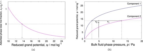
and we obtain p1=2.59899 and p2=13.0167 Pa. The adsorbed-phase mole fractions x1 and x2 are

x1=y1*p/p1

x2=y2*p/p2

and we obtain x1 = 0.769531 and x2 = 0.230472, graphically depicted in Figure 2(b). With psi and x1 and x2, the total adsorbed amount, qT, can be calculated

qT = 1.0/(0.769531/(qs1*b1*p1^nu1/(1.0+b1*p1^nu1))+

  (0.230472/(qs2*b2*p2^nu2/(1.0+b2*p2^nu2))))

leading to qT = 5.09176 mol/(kg framework).

q1 = x1*qT

q2 = x2*qT

and we have q1 = 3.91827 and q2 = 1.17351 mol/(kg framework).

Using the following Mathematica code, we can generate the IAST prediction as a function of pressure

pressurebegin = 10^(-4);

pressureend = 10^10;

numberpoints = 100;

For[i = 1, i <= numberpoints, i++,

 p = 10^(((Log10[pressureend] - Log10[pressurebegin])*

   (i/(numberpoints - 1.0))) + Log10[pressurebegin]);

 root = psi /.

  FindRoot[

   y1*p/((1.0/(b1^(1.0/nu1)))*(Exp[nu1 psi/(qs1)] - 1.0)^(1.0/nu1)) +

  y2*p/((1.0/(b2^(1.0/nu2)))*(Exp[nu2 psi/(qs2)] - 1.0)^(1.0/

    nu2)) - 1.0, {psi, 10}];

p1 = (1.0/(b1^(1.0/nu1)))*(Exp[nu1*root/qs1] - 1.0)^(1/nu1);

p2 = (1.0/(b2^(1.0/nu2)))*(Exp[nu2*root/qs2] - 1.0)^(1/nu2);

x1 = y1*P/((1.0/(b1^(1.0/nu1)))*(Exp[nu1*root/qs1] - 1.0)^(1.0/nu1));

x2 = y2*P/((1.0/(b2^(1.0/nu2)))*(Exp[nu2*root/qs2] - 1.0)^(1.0/nu2));

qT = 1.0/(x1/(qs1*b1*p1^nu1/(1 + b1*p1^nu1)) +

   x2/(qs2*b2*p2^nu2/(1 + b2*p2^nu2)));

 Print[p, “ ”, x1*qT, “ ”, x2*qT]]

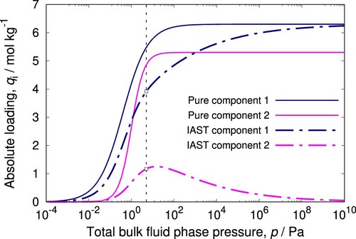
The result is plotted in Figure 3 which shows pure component and mixture isotherms for a binary mixture. Adsorption for the component with the highest saturation loading dominates at high pressures.

Figure 3. (Colour online) Example of IAST prediction for a binary mixture described by Langmuir-Freundlich isotherms. At 5 Pa total pressure and gas-phase mole fractions $y_1=0.4$ and $y_2=0.6$, we find adsorbed absolute loadings of $q_1=3.92$ and $q_2=1.17$ mol/kg. Typically in a mixture, a component with the highest saturation loading will drive the other components out at high pressures.

3.4. Analytic mixture prediction methods

3.4.1. Multi-component Langmuir

In the book of Do [23], the multi-component Langmuir is derived from the IAST equations. Equations (47(47) $y_i{p}_{{}_T}=p_i=x_i{p}_i^{\ast }\left(\psi \right)i=1,2,\dots ,N_{{}_C}\left(N_{{}_C}\mathrm{e}\mathrm{q}\mathrm{u}\mathrm{a}\mathrm{t}\mathrm{i}\mathrm{o}\mathrm{n}\mathrm{s}\right)$(47) ) and (48(48) $\sum _{i=1}^{N_{{}_C}}{x}_i=1\left(1\mathrm{e}\mathrm{q}\mathrm{u}\mathrm{a}\mathrm{t}\mathrm{i}\mathrm{o}\mathrm{n}\right)$(48) ) can be combined to yield [104] (56) $\sum _{i=1}^{N_{{}_C}}\frac{p_i}{p_i^{\ast }}=\sum _{i=1}^{N_{{}_C}}{x}_i=1$(56) This closure equation can be used to reduce the problem to a single nonlinear algebraic equation in ψ: (57) $\frac{p_1}{p_1^{\ast }\left(\psi \right)}+\cdots +\frac{p_{N_{{}_C}}}{p_{N_{{}_C}}^{\ast }\left(\psi \right)}=1$(57) We can then use the expressions for the pure component sorption pressure $\left(p_i^{\ast }\right)$ and use these as input in Equation (57(57) $\frac{p_1}{p_1^{\ast }\left(\psi \right)}+\cdots +\frac{p_{N_{{}_C}}}{p_{N_{{}_C}}^{\ast }\left(\psi \right)}=1$(57) ). For the single component Langmuir isotherm (58) $q_i=q^{\mathrm{s}\mathrm{a}\mathrm{t}}\frac{b_i{p}_i}{1+b_i{p}_i}$(58) we obtain (59) $\psi \left(p^{\ast }\right)={\int }_0^p\frac{q\left(p\right)}{p}\mathrm{d}p=q^{\mathrm{s}\mathrm{a}\mathrm{t}}{\int }_0^{p^{\ast }}\frac{b}{1+bp}\mathrm{d}p=q^{\mathrm{s}\mathrm{a}\mathrm{t}}\ln [1+b{p}^{\ast }]$(59) Inverting this equation, we have (60) $p^{\ast }\left(\psi \right)=\frac{\exp \left[\frac{\psi }{q^{\mathrm{s}\mathrm{a}\mathrm{t}}}\right]-1}{b}$(60) Filling this into Equation (57(57) $\frac{p_1}{p_1^{\ast }\left(\psi \right)}+\cdots +\frac{p_{N_{{}_C}}}{p_{N_{{}_C}}^{\ast }\left(\psi \right)}=1$(57) ), we obtain (61) $\frac{b_1{p}_1}{\exp \left(\frac{\psi }{q_1^{\mathrm{s}\mathrm{a}\mathrm{t}}}\right)-1}+\frac{b_2{p}_2}{\exp \left(\frac{\psi }{q_2^{\mathrm{s}\mathrm{a}\mathrm{t}}}\right)-1}=1$(61) which can be analytically solved for ψ when the saturation capacities $q_1^{\mathrm{s}\mathrm{a}\mathrm{t}}$ and $q_2^{\mathrm{s}\mathrm{a}\mathrm{t}}$ are equal. (62) $\exp \left(\frac{\psi }{q^{\mathrm{s}\mathrm{a}\mathrm{t}}}\right)=1+b_1{p}_1+b_2{p}_2$(62) Using this in Equation (60(60) $p^{\ast }\left(\psi \right)=\frac{\exp \left[\frac{\psi }{q^{\mathrm{s}\mathrm{a}\mathrm{t}}}\right]-1}{b}$(60) ) we find the sorption pressures (63) $p_i^{\ast }\left(\psi \right)=\frac{b_1{p}_1+b_2{p}_2}{b_i}$(63) Substituting the sorption pressures into Raoult's law Equation (47(47) $y_i{p}_{{}_T}=p_i=x_i{p}_i^{\ast }\left(\psi \right)i=1,2,\dots ,N_{{}_C}\left(N_{{}_C}\mathrm{e}\mathrm{q}\mathrm{u}\mathrm{a}\mathrm{t}\mathrm{i}\mathrm{o}\mathrm{n}\mathrm{s}\right)$(47) ), we obtain the adsorbed phase mole fractions (64) $x_i=\frac{b_i{p}_i}{b_1{p}_1+b_2{p}_2}$(64) The total amount adsorbed is obtained by substituting Equation (58(58) $q_i=q^{\mathrm{s}\mathrm{a}\mathrm{t}}\frac{b_i{p}_i}{1+b_i{p}_i}$(58) ), (63(63) $p_i^{\ast }\left(\psi \right)=\frac{b_1{p}_1+b_2{p}_2}{b_i}$(63) ), and (64(64) $x_i=\frac{b_i{p}_i}{b_1{p}_1+b_2{p}_2}$(64) ) into Equation (50(50) $\frac{1}{q_{{}_T}}=\sum _{i=1}^{N_{{}_C}}\frac{x_i}{q_i^{\ast }}$(50) ) (65) $q_T=q^{\mathrm{s}\mathrm{a}\mathrm{t}}\frac{b_1{p}_1+b_2{p}_2}{1+b_1{p}_1+b_2{p}_2}$(65) and the adsorbed amount contributed by the component i is (66) $q_i=q^{\mathrm{s}\mathrm{a}\mathrm{t}}\frac{b_i{p}_i}{1+b_1{p}_1+b_2{p}_2}i=1,2$(66) which is the extended Langmuir equation (Equation (33(33) $q_i=\frac{q_i^{\mathrm{s}\mathrm{a}\mathrm{t}}{b}_i{p}_i}{1+\sum _{j=1}^{N_{{}_C}}{b}_j{p}_j}$(33) )) with equal saturation capacities.

3.4.2. Analytic Taylor series expansions of LeVan and Vermeulen [105]

Le Van and Vermeulen [105] derived the explicit isotherms for binary mixtures from the Gibbs adsorption isotherm. These authors considered single site Langmuir and Freundlich isotherms for the pure components. However, this method can be extended to any kind of pure component isotherms, provided these isotherms have an explicit expression for the reduced grand potential $\left(\psi \right)$ in terms of pure component pressure $\left(p_i^{\ast }\right)$. This method is applicable for cases where the saturation capacities of the components are close to each other [23]. The derivation is as follows:

According to IAST, the reduced grand potential for pure component i is $\left({\psi }_i\right)$ is expressed as (67) ${\psi }_i={\int }_0^{p_i^{\ast }}\frac{q_i}{p_i}\mathrm{d}{p}_i$(67) Also, the reduced grand potential of the mixture $\left({\psi }^{\mathrm{m}\mathrm{i}\mathrm{x}}\right)$ is considered to be equal to the pure-component grand potential $\left({\psi }_i\right)$ at pressure, $p_i^{\ast }$ for component i and the temperature of the mixture, i.e. (68) ${\psi }_i=q_i^{\mathrm{s}\mathrm{a}\mathrm{t}}\ln (1+b_{i,1}{p}_i^{\ast }+b_{i,2}{\left(p_i^{\ast }\right)}^2)$(68) For the ideal adsorbed solution, the partial pressures and the adsorbed phase composition are related by Raoult's law analogy.

(69) $p_i=x_i{p}_i^{\ast }\left(\psi \right)$(69) In Equation (69(69) $p_i=x_i{p}_i^{\ast }\left(\psi \right)$(69) ), $p_i^{\ast }$ is the pure component pressure in equilibrium with an adsorbed phase of the component i at the reduced grand potential $\left(\psi \right)$ and temperature of the mixture. $p_i$ is the partial pressure of component i and $x_i$ is the mole fraction in the adsorbed phase. Using the relation $\sum _i^{N_{{}_C}}{x}_i=1$ and substituting $x_i$ using Equation (69(69) $p_i=x_i{p}_i^{\ast }\left(\psi \right)$(69) ) yields (70) $\frac{p_1}{p_1^{\ast }}+\frac{p_2}{p_2^{\ast }}=1$(70) The single component isotherms (Langmuir and Freundlich) are substituted into Equation (67(67) ${\psi }_i={\int }_0^{p_i^{\ast }}\frac{q_i}{p_i}\mathrm{d}{p}_i$(67) ) which on integration yields expressions for pure component pressures $(p_1^{\ast },p_2^{\ast })$. These expressions are used to further substitute $p_1^{\ast }$ and $p_2^{\ast }$ in Equation (70(70) $\frac{p_1}{p_1^{\ast }}+\frac{p_2}{p_2^{\ast }}=1$(70) ). The resulting expression, which is a function of $p_1$, $p_2$ and ψ is expanded using Taylor series to obtain an explicit expression. The reduced grand potential ψ is differentiated to calculate the binary isotherms. (71) $q_i=p_i\frac{\mathrm{\partial }\psi }{\mathrm{\partial }{p}_i}$(71) Le Van and Vermeulen [105] derived the expressions for binary mixtures where both components either obey Langmuir, or Freundlich isotherms in their pure form.

(1)

Langmuir Isotherms For pure component i, the reduced grand potential $\left({\psi }_i\right)$ equals: (72) $\psi =q_i^{\mathrm{s}\mathrm{a}\mathrm{t}}\ln (1+b_i{p}_i^{\ast })$(72) (73) $p_i^{\ast }=\frac{1}{b_i}[\exp \left(\frac{\psi }{q_i^{\mathrm{s}\mathrm{a}\mathrm{t}}}\right)-1]$(73) $p_1^{\ast }$ and $p_2^{\ast }$ in Equation (70(70) $\frac{p_1}{p_1^{\ast }}+\frac{p_2}{p_2^{\ast }}=1$(70) ) are substituted using Equation (73(73) $p_i^{\ast }=\frac{1}{b_i}[\exp \left(\frac{\psi }{q_i^{\mathrm{s}\mathrm{a}\mathrm{t}}}\right)-1]$(73) ), which yields (74) $\frac{b_1{p}_1}{\exp \left(\frac{\psi }{q_1^{\mathrm{s}\mathrm{a}\mathrm{t}}}\right)-1}+\frac{b_2{p}_2}{\exp \left(\frac{\psi }{q_2^{\mathrm{s}\mathrm{a}\mathrm{t}}}\right)-1}=1$(74) Since the reduced grand potentials for the pure components are equal to the mixture (Equation (68(68) ${\psi }_i=q_i^{\mathrm{s}\mathrm{a}\mathrm{t}}\ln (1+b_{i,1}{p}_i^{\ast }+b_{i,2}{\left(p_i^{\ast }\right)}^2)$(68) )), ψ will be used as the grand potential for both the components. To proceed with the derivation, the following parameters are defined: (75) $q^{\mathrm{s}\mathrm{a}\mathrm{t}}=\frac{q_1^{\mathrm{s}\mathrm{a}\mathrm{t}}+q_2^{\mathrm{s}\mathrm{a}\mathrm{t}}}{2}$(75) (76) $ϵ=\frac{q_1^{\mathrm{s}\mathrm{a}\mathrm{t}}-q_2^{\mathrm{s}\mathrm{a}\mathrm{t}}}{2q^{\mathrm{s}\mathrm{a}\mathrm{t}}}$(76) Combining Equations (75(75) $q^{\mathrm{s}\mathrm{a}\mathrm{t}}=\frac{q_1^{\mathrm{s}\mathrm{a}\mathrm{t}}+q_2^{\mathrm{s}\mathrm{a}\mathrm{t}}}{2}$(75) ) and (76(76) $ϵ=\frac{q_1^{\mathrm{s}\mathrm{a}\mathrm{t}}-q_2^{\mathrm{s}\mathrm{a}\mathrm{t}}}{2q^{\mathrm{s}\mathrm{a}\mathrm{t}}}$(76) ) yields (77) $q_1^{\mathrm{s}\mathrm{a}\mathrm{t}}=q^{\mathrm{s}\mathrm{a}\mathrm{t}}(1+ϵ)$(77) (78) $q_2^{\mathrm{s}\mathrm{a}\mathrm{t}}=q^{\mathrm{s}\mathrm{a}\mathrm{t}}(1-ϵ)$(78) Now, Equation (74(74) $\frac{b_1{p}_1}{\exp \left(\frac{\psi }{q_1^{\mathrm{s}\mathrm{a}\mathrm{t}}}\right)-1}+\frac{b_2{p}_2}{\exp \left(\frac{\psi }{q_2^{\mathrm{s}\mathrm{a}\mathrm{t}}}\right)-1}=1$(74) ) is expanded using the Taylor series for ψ about $ϵ=0$. (79) $\psi ={\psi |}_{ϵ=0}+{\frac{ϵ}{1!}\frac{\mathrm{d}\psi }{\mathrm{d}ϵ}|}_{ϵ=0}+{\frac{{ϵ}^2}{2!}\frac{{\mathrm{d}}^2\psi }{\mathrm{d}{ϵ}^2}|}_{ϵ=0}+\cdots$(79) Le Van and Vermeulen obtained isotherms for the binary mixture components using the Taylor expansion of Equation (74(74) $\frac{b_1{p}_1}{\exp \left(\frac{\psi }{q_1^{\mathrm{s}\mathrm{a}\mathrm{t}}}\right)-1}+\frac{b_2{p}_2}{\exp \left(\frac{\psi }{q_2^{\mathrm{s}\mathrm{a}\mathrm{t}}}\right)-1}=1$(74) ). The isotherms are calculated using Equation (71(71) $q_i=p_i\frac{\mathrm{\partial }\psi }{\mathrm{\partial }{p}_i}$(71) ). The grand potential $\left(\psi \right)$ is as follows (80) $\psi =q^{\mathrm{s}\mathrm{a}\mathrm{t}}\ln (1+b_1{p}_1+b_2{p}_2)$(80) In Equation (80(80) $\psi =q^{\mathrm{s}\mathrm{a}\mathrm{t}}\ln (1+b_1{p}_1+b_2{p}_2)$(80) ), $q^{\mathrm{s}\mathrm{a}\mathrm{t}}$ is the average saturation loading which depends on the nature of the Taylor expansion (i.e. the number of terms considered in the expansion). These authors have derived explict isotherms by considering two, and three terms Taylor series expansion of ψ. (A) Two term expansion: (81) $q^{\mathrm{s}\mathrm{a}\mathrm{t}}=\frac{q_1^{\mathrm{s}\mathrm{a}\mathrm{t}}{b}_1{p}_1+q_2^{\mathrm{s}\mathrm{a}\mathrm{t}}{b}_2{p}_2}{b_1{p}_1+b_2{p}_2}$(81) (82) $q_1^{\mathrm{s}\mathrm{a}\mathrm{t}}=q^{\mathrm{s}\mathrm{a}\mathrm{t}}\frac{b_1{p}_1}{1+b_1{p}_1+b_2{p}_2}+{\mathrm{\Delta }}_{\mathrm{L}2}$(82) where (83) ${\mathrm{\Delta }}_{\mathrm{L}2}=(q_1^{\mathrm{s}\mathrm{a}\mathrm{t}}-q_2^{\mathrm{s}\mathrm{a}\mathrm{t}})\frac{b_1{b}_2{p}_1{p}_2}{{(b_1{p}_1+b_2{p}_2)}^2}\ln (1+b_1{p}_1+b_2{p}_2)$(83) (B) Three term expansion: (84) $\begin{array}{rl}{q}^{\mathrm{s}\mathrm{a}\mathrm{t}}& =\frac{b_1{p}_1{q}_1^{\mathrm{s}\mathrm{a}\mathrm{t}}+b_2{p}_2{q}_2^{\mathrm{s}\mathrm{a}\mathrm{t}}}{b_1{p}_1+b_2{p}_2}+2\frac{{(q_1^{\mathrm{s}\mathrm{a}\mathrm{t}}-q_2^{\mathrm{s}\mathrm{a}\mathrm{t}})}^2}{q_1^{\mathrm{s}\mathrm{a}\mathrm{t}}+q_2^{\mathrm{s}\mathrm{a}\mathrm{t}}}\frac{b_1{b}_2{p}_1{p}_2}{{(b_1{p}_1+b_2{p}_2)}^2}\\ & \times [(\frac{1}{b_1{p}_1+b_2{p}_2}+\frac{1}{2})\ln (1+b_1{p}_1+b_2{p}_2)-1]\end{array}$(84) (85) $q_1^{\mathrm{s}\mathrm{a}\mathrm{t}}=q^{\mathrm{s}\mathrm{a}\mathrm{t}}\frac{b_1{p}_1}{1+b_1{p}_1+b_2{p}_2}+{\mathrm{\Delta }}_{\mathrm{L}2}(1+{\mathrm{\Delta }}_{\mathrm{L}3})$(85) where (86) $\begin{array}{rl}{\mathrm{\Delta }}_{\mathrm{L}3}& =\frac{q_1^{\mathrm{s}\mathrm{a}\mathrm{t}}-q_2^{\mathrm{s}\mathrm{a}\mathrm{t}}}{q_1^{\mathrm{s}\mathrm{a}\mathrm{t}}+q_2^{\mathrm{s}\mathrm{a}\mathrm{t}}}\frac{1}{b_1{p}_1+b_2{p}_2}\\ & [\frac{{\left(b_2{p}_2\right)}^2+2\left(b_2{p}_2\right)-4\left(b_1{p}_1\right)-{\left(b_1{p}_1\right)}^2}{b_1{p}_1+b_2{p}_2}\ln (1+b_1{p}_1+b_2{p}_2)\\ & +\frac{3{\left(b_1{p}_1\right)}^2+4\left(b_1{p}_1\right)+b_1{b}_2{p}_1{p}_2-2\left(b_2{p}_2\right)-2{\left(b_2{p}_2\right)}^2}{1+b_1{p}_1+b_2{p}_2}]\end{array}$(86) The multi-component adsorption isotherm for component 2 can be obtained by simply interchanging the subscripts 1, and 2 in the above equations.

(2)

Freundlich Isotherm An approach similar to the above case is applied to a binary mixture where the pure components obey the Freundlich isotherm which is shown below (87) $q_i^{\mathrm{s}\mathrm{a}\mathrm{t}}=b_i{p}^{{\nu }_i}$(87) The reduced grand potential $\left(\psi \right)$ equation in terms of the partial pressure is (88) ${\left(\frac{b_1}{{\nu }_1}\right)}^{1/{\nu }_1}{p}_1\exp (-\frac{1}{{\nu }_1}\ln \psi )+{\left(\frac{b_2}{{\nu }_2}\right)}^{1/{\nu }_2}{p}_2\exp (-\frac{2}{{\nu }_2}\ln \psi )=1$(88) For unequal Freundlich exponents $\left({\nu }_i\right)$ but very close to each other, the value of ψ can be computed using the Taylor series expansion. The expression for the adsorbed loadings for the components in the mixture are derived using the Taylor series expansion of ψ about ϵ (Equation (79(79) $\psi ={\psi |}_{ϵ=0}+{\frac{ϵ}{1!}\frac{\mathrm{d}\psi }{\mathrm{d}ϵ}|}_{ϵ=0}+{\frac{{ϵ}^2}{2!}\frac{{\mathrm{d}}^2\psi }{\mathrm{d}{ϵ}^2}|}_{ϵ=0}+\cdots$(79) )). For Freundlich isotherms, ϵ is (89) $ϵ=\frac{{\nu }_1-{\nu }_2}{{\nu }_1+{\nu }_2}$(89) In Equation (89(89) $ϵ=\frac{{\nu }_1-{\nu }_2}{{\nu }_1+{\nu }_2}$(89) ), ${\nu }_1$ and ${\nu }_2$ are the Freundlich exponents for component 1 and 2 respectively. The expression for the adsorbed loading for component 1 $\left(q_1\right)$ is shown below, a detailed derivation for which can be found in Ref. [105]. (90) $q_1=\frac{\overline{\nu }{\left(\frac{b_1}{{\nu }_1}\right)}^{1/{\nu }_1}{p}_1}{{[{\left(\frac{b_1}{{\nu }_1}\right)}^{1/{\nu }_1}{p}_1+{\left(\frac{b_2}{{\nu }_2}\right)}^{1/{\nu }_2}{p}_2]}^{1-\overline{\nu }}}+{\mathrm{\Delta }}_{\mathrm{F}2}$(90) where (91) $\begin{array}{rl}{\mathrm{\Delta }}_{\mathrm{F}2}=& ({\nu }_1-{\nu }_2)\frac{{\left(\frac{b_1}{{\nu }_1}\right)}^{1/{\nu }_1}{p}_1{\left(\frac{b_2}{{\nu }_2}\right)}^{1/{\nu }_2}{p}_2}{{[{\left(\frac{b_1}{{\nu }_1}\right)}^{1/{\nu }_1}{p}_1+{\left(\frac{b_2}{{\nu }_2}\right)}^{1/{\nu }_2}{p}_2]}^{2-\nu }}\\ \left(91\right)& & \times \ln [{\left(\frac{b_1}{{\nu }_1}\right)}^{1/{\nu }_1}{p}_1+{\left(\frac{b_2}{{\nu }_2}\right)}^{1/{\nu }_2}{p}_2]\end{array}$(91) (92) $\overline{\nu }=\frac{{\nu }_1{\left(\frac{b_1}{{\nu }_1}\right)}^{1/{\nu }_1}{p}_1+{\nu }_2{\left(\frac{b_2}{{\nu }_2}\right)}^{1/{\nu }_2}{p}_2}{{\left(\frac{b_1}{{\nu }_1}\right)}^{1/{\nu }_1}{p}_1+{\left(\frac{b_2}{{\nu }_2}\right)}^{1/{\nu }_2}{p}_2}$(92)

3.4.3. Analytic approach of Ilic et al. [106]

Ilic et al. [106] derived an explicit competitive isotherm model for binary mixtures, where the pure components obey quadratic isotherms. For pure components, the reduced grand potential is (93) ${\psi }_i=q_i^{\mathrm{s}\mathrm{a}\mathrm{t}}\ln (1+b_{i,1}{p}_i^{\ast }+b_{i,2}{\left(p_i^{\ast }\right)}^2)$(93) The grand potential of the mixture is considered to be equal to the pure-component grand potential $\left({\psi }_i\right)$ at pressure, $p_i^{\ast }$ for component i and the temperature of the mixture, i.e. (94) $\psi ={\psi }_1={\psi }_2$(94) Using Equations (93(93) ${\psi }_i=q_i^{\mathrm{s}\mathrm{a}\mathrm{t}}\ln (1+b_{i,1}{p}_i^{\ast }+b_{i,2}{\left(p_i^{\ast }\right)}^2)$(93) ), and (94(94) $\psi ={\psi }_1={\psi }_2$(94) ) and considering the saturation capacities of the components to be equal $(q_1^{\mathrm{s}\mathrm{a}\mathrm{t}}=q_2^{\mathrm{s}\mathrm{a}\mathrm{t}})$, we obtain (95) $\ln (1+b_{1,1}{p}_1^{\ast }+b_{1,2}{\left(p_1^{\ast }\right)}^2)=\ln (1+b_{2,1}{p}_1^{\ast }+b_{2,2}{\left(p_1^{\ast }\right)}^2)$(95) In Equation (95(95) $\ln (1+b_{1,1}{p}_1^{\ast }+b_{1,2}{\left(p_1^{\ast }\right)}^2)=\ln (1+b_{2,1}{p}_1^{\ast }+b_{2,2}{\left(p_1^{\ast }\right)}^2)$(95) ), $b_{i,j}$ represents equilibrium constant. This equation can be reformulated using a cubic polynomial which is defined as a function of the adsorbed mole fraction of component 1 $\left(x_1\right)$. (96) $F(p_1,p_2,x_1)=A(p_1,p_2)x_1^3+B(p_1,p_2)x_1^2+C(p_1,p_2)x_1+D(p_1,p_2)$(96) where (97) $A(p_1,p_2)=\alpha p_1+p_1>0$(97) (98) $B(p_1,p_2)=p_1(\text{β}{p}_1-2\alpha )-p_2(1+\gamma p_2)$(98) (99) $C(p_1,p_2)=p_1(\alpha -2\text{β}{p}_1)$(99) (100) $D\left(p_1\right)=\text{β}{p}_1^2$(100) (101) $\alpha =\frac{b_{1,1}}{b_{2,1}}>0$(101) (102) $\text{β}=\frac{b_{1,2}}{b_{2,1}}\ge 0$(102) (103) $\gamma =\frac{b_{2,2}}{b_{2,1}}\ge 0$(103) (104) $b_{i,1}>0,i=1,2$(104) (105) $b_{i,2}\ge 0,i=1,2$(105) The root $\left(x_1\right)$ of this cubic polynomial (Equation (96(96) $F(p_1,p_2,x_1)=A(p_1,p_2)x_1^3+B(p_1,p_2)x_1^2+C(p_1,p_2)x_1+D(p_1,p_2)$(96) )) can be derived analytically by applying the formulae of Cardano [107]. The problem is solved by selecting the physically meaningful root out of the three obtained roots. Once the value of $x_1$ is computed, the adsorbed loading for component i $\left(q_i\right)$ is calculated using the following expression [77]: (106) $q_i=[\frac{x_1}{q_1^{\ast }\left(p_1^{\ast }\right)}+\frac{1-x_1}{q_2^{\ast }\left(p_2^{\ast }\right)}]x_i$(106) In Equation (106(106) $q_i=[\frac{x_1}{q_1^{\ast }\left(p_1^{\ast }\right)}+\frac{1-x_1}{q_2^{\ast }\left(p_2^{\ast }\right)}]x_i$(106) ), $x_i$ is the adsorbed mole fraction of component i, $q_i^{\ast }$ is the adsorbed loading for pure component i, and $p_i^{\ast }$ is the corresponding gas phase pressure.

3.4.4. Analytic approach of Tarafder and Mazzotti [63]

Tarafder and Mazzotti obtained explicit isotherms for binary mixtures using IAST, where the pure components obey Langmuir-, anti-Langmuir- [24], Brunauer-Emmett-Teller (BET)-, and quadratic-type adsorption isotherms. These mixture isotherms are valid only when the saturation capacities of the components are identical $(q_1^{\mathrm{s}\mathrm{a}\mathrm{t}}=q_2^{\mathrm{s}\mathrm{a}\mathrm{t}}=q^{\mathrm{s}\mathrm{a}\mathrm{t}})$.

Assuming both the fluid and the adsorbed phase as ideal (107) $p_i=p_i^{\ast }{x}_i(i=1,2)$(107) $p_i$ is the concentration of component i in the mixture, $p_i^{\ast }$ is the pure component concentration, and $q_i^{\mathrm{s}\mathrm{a}\mathrm{t}}$ is the saturation loading in Equation (107(107) $p_i=p_i^{\ast }{x}_i(i=1,2)$(107) ). Explicit solutions for the adsorbed phase mole fractions $\left(x_1\mathrm{a}\mathrm{n}\mathrm{d}{x}_2\right)$ are derived from (108) $\psi \left(\frac{p_1}{x_1}\right)=\psi \left(\frac{p_1}{x_2}\right)$(108) (109) $x_1+x_2=1$(109) The reduced grand potentials $\left(\psi \right)$ for component i, computed based on the above mentioned single component isotherms are as follows:

• Langmuir (110) ${\psi }_i=q_i^{\mathrm{s}\mathrm{a}\mathrm{t}}\ln (1+b_i{p}_i^{\ast })$(110)

• Anti-Langmuir (111) ${\psi }_i=-q_i^{\mathrm{s}\mathrm{a}\mathrm{t}}\ln (1-b_i{p}_i^{\ast })$(111)

• BET (112) ${\psi }_i=q_i^{\mathrm{s}\mathrm{a}\mathrm{t}}\ln \left(\frac{1-(b_{i,1}{p}_i^{\ast }+b_{i,2}{p}_i^{\ast })}{1-b_{i,2}{p}_i^{\ast }}\right)$(112)

• Quadratic (113) ${\psi }_i=q_i^{\mathrm{s}\mathrm{a}\mathrm{t}}\ln (1+b_{i,1}{p}_i^{\ast }+b_{i,2}{p_i^{\ast }}^2)$(113)

In Equations (110(110) ${\psi }_i=q_i^{\mathrm{s}\mathrm{a}\mathrm{t}}\ln (1+b_i{p}_i^{\ast })$(110) ) and (111(111) ${\psi }_i=-q_i^{\mathrm{s}\mathrm{a}\mathrm{t}}\ln (1-b_i{p}_i^{\ast })$(111) ), $b_i$ is the equilibrium constant. Similarly, in Equations (112(112) ${\psi }_i=q_i^{\mathrm{s}\mathrm{a}\mathrm{t}}\ln \left(\frac{1-(b_{i,1}{p}_i^{\ast }+b_{i,2}{p}_i^{\ast })}{1-b_{i,2}{p}_i^{\ast }}\right)$(112) ) and (113(113) ${\psi }_i=q_i^{\mathrm{s}\mathrm{a}\mathrm{t}}\ln (1+b_{i,1}{p}_i^{\ast }+b_{i,2}{p_i^{\ast }}^2)$(113) ), $b_{i,j}(j=1,2)$ represents the equilibrium constants. The adsorbed mole fraction of component 1 $\left(x_1\right)$, and the total adsorbed loading $(q_{{}_T}=q_1+q_2)$ are calculated for different cases depending on the type of single component isotherms followed by each component in the mixture.

(1)	Quadratic isotherm (component 1) and BET isotherm (component 2) (114) $\frac{x_1}{p_1}=\begin{array}{r}\frac{(b_{1,1}(1-b_{2,2}{p}_1)-b_{1,2}{p}_1)+\sqrt{{(b_{1,1}(1-b_{2,2}{p}_1)-b_{1,2}{p}_1)}^2+4b_{1,2}(b_{1,1}{p}_1+b_{2,1}{p}_1)(1-b_{2,2}{p}_1)}}{2(b_{1,1}{p}_1+b_{2,1}{p}_1)}\end{array}$(114) (115) $\begin{array}{rl}& q_{{}_T}=q^{\mathrm{s}\mathrm{a}\mathrm{t}}{[\frac{x_1(x_1^2+b_{1,1}{p}_1{x}_1+b_{1,2}{p}_1^2)}{(b_{1,1}{x}_1+2b_{1,2}{p}_1)p_1}+\frac{(x_2-b_{2,2}{p}_1)(x_2-b_{2,2}{p}_1+b_{2,1}{p}_1)}{b_{2,1}{p}_1}]}^{-1}\end{array}$(115)
(2)	Quadratic isotherm (component 1) and Langmuir isotherm (component 2) (116) $\frac{x_1}{p_1}=\frac{(b_{1,1}-b_{1,2}{p}_1)+\sqrt{{(b_{1,1}-b_{1,2}{p}_1)}^2+4b_{1,2}(b_{1,1}{p}_1+b_2{p}_1)}}{2(b_{1,1}{p}_1+b_2{p}_1)}$(116) (117) $q_{{}_T}=q^{\mathrm{s}\mathrm{a}\mathrm{t}}{[\frac{x_1(x_1^2+b_{1,1}{p}_1{x}_1+b_{1,2}{p}_1^2)}{(b_{1,1}{x}_1+2b_{1,2}{p}_1)p_1}+\frac{x_2(x_2+b_2{p}_1)}{b_2{p}_1}]}^{-1}$(117)
(3)	Quadratic isotherm (component 1) and anti-Langmuir isotherm (component 2) (118) $\frac{x_1}{p_1}=\frac{(b_{1,1}(1-b_2{p}_1)-b_{1,2}{p}_1)+\sqrt{{(b_{1,1}(1-b_2{p}_1)-b_{1,2}{p}_1)}^2+4b_{1,2}(b_{1,1}{p}_1+b_2{p}_1)(1-b_2{p}_1)}}{2(b_{1,1}{p}_1+b_2{p}_1)}$(118) (119) $q_{{}_T}=q^{\mathrm{s}\mathrm{a}\mathrm{t}}{[\frac{x_1(x_1^2+b_{1,1}{p}_1{x}_1+b_{1,2}{p}_1^2)}{(b_{1,1}{x}_1+2b_{1,2}{p}_1)p_1}+\frac{x_2(x_2-b_2{p}_1)}{b_2{p}_1}]}^{-1}$(119)

3.4.5. Analytic approach of Van Assche et al. [30] (Implemented in RUPTURA)

Van Assche et al. [30] derived an explicit multi-component adsorption model for arbitrary number of components. This model accounts for the effects of the size of the adsorbing components. The explicit isotherms (EI) are derived using the concepts of statistical mechanics. In this model, the components are arranged based on their saturation capacities as shown below. (120) $q_{N_{{}_C}}^{\mathrm{s}\mathrm{a}\mathrm{t}}\ge q_{N_{{}_C}-1}^{\mathrm{s}\mathrm{a}\mathrm{t}}\ge \cdots \ge q_2^{\mathrm{s}\mathrm{a}\mathrm{t}}\ge q_1^{\mathrm{s}\mathrm{a}\mathrm{t}}$(120) The largest component or the one with the smallest saturation capacity is considered to adsorb first. The adsorbent is considered to be a lattice divided into grids of uniform size. Once, the adsorption of the 1st component takes place, the remaining lattice is further subdivided such that the component with the next smallest saturation capacity adsorbs. The process continues until the last component adsorbs. While dividing the lattice each time into uniform grids, the grid size is taken to be the ratio of the saturation capacities of the corresponding component and its preceding counter-part $\left(q_i^{\mathrm{s}\mathrm{a}\mathrm{t}}/q_{i-1}^{\mathrm{s}\mathrm{a}\mathrm{t}}\right)$. The adsorption isotherm for component i in a mixture of $N_{{}_C}$ components is [30]: (121) $q_i=\left(q_i^{\mathrm{s}\mathrm{a}\mathrm{t}}{b}_i{p}_i\right)\frac{1}{\text{β}}\prod _{k=1}^i{\alpha }_k$(121) where

(122) ${\alpha }_1=1$(122) (123) ${\alpha }_i={[{(\cdots {({({(1+b_{N_{{}_C}}{p}_{N_{{}_C}})}^{\frac{q_{N_{{}_C}}^{\mathrm{s}\mathrm{a}\mathrm{t}}}{q_{N_{{}_C}-1}^{\mathrm{s}\mathrm{a}\mathrm{t}}}}+b_{N_{{}_C}-1}{p}_{N_{{}_C}-1})}^{\frac{q_{N_{{}_C}-1}^{\mathrm{s}\mathrm{a}\mathrm{t}}}{q_{N_{{}_C}-2}^{\mathrm{s}\mathrm{a}\mathrm{t}}}}+b_{N_{{}_C}-2}{p}_{N_{{}_C}-2})}^{\frac{q_{N_{{}_C}-2}^{\mathrm{s}\mathrm{a}\mathrm{t}}}{q_{N_{{}_C}-3}^{\mathrm{s}\mathrm{a}\mathrm{t}}}}\cdots +b_{i+1}{p}_{i+1})}^{\frac{q_{i+1}^{\mathrm{s}\mathrm{a}\mathrm{t}}}{q_i^{\mathrm{s}\mathrm{a}\mathrm{t}}}}+b_i{p}_i]}^{\frac{q_i^{\mathrm{s}\mathrm{a}\mathrm{t}}}{q_{i-1}^{\mathrm{s}\mathrm{a}\mathrm{t}}}-1}$(123)

(124) $\text{β}=[{(\cdots {({({(1+b_{N_{{}_C}}{p}_{N_{{}_C}})}^{\frac{q_{N_{{}_C}}^{\mathrm{s}\mathrm{a}\mathrm{t}}}{q_{N_{{}_C}-1}^{\mathrm{s}\mathrm{a}\mathrm{t}}}}+b_{N_{{}_C}-1}{p}_{N_{{}_C}-1})}^{\frac{q_{N_{{}_C}-1}^{\mathrm{s}\mathrm{a}\mathrm{t}}}{q_{N_{{}_C}-2}^{\mathrm{s}\mathrm{a}\mathrm{t}}}}+b_{N_{{}_C}-2}{p}_{N_{{}_C}-2})}^{\frac{q_{N_{{}_C}-2}^{\mathrm{s}\mathrm{a}\mathrm{t}}}{q_{N_{{}_C}-3}^{\mathrm{s}\mathrm{a}\mathrm{t}}}}\cdots +b_2{p}_2)}^{\frac{q_2^{\mathrm{s}\mathrm{a}\mathrm{t}}}{q_1^{\mathrm{s}\mathrm{a}\mathrm{t}}}}+b_1{p}_1]$(124) For a binary model, the equations read (125) $q_1=q_1^{\mathrm{s}\mathrm{a}\mathrm{t}}\frac{b_1{p}_1}{{(1+b_2{p}_2)}^{\frac{q_2^{\mathrm{s}\mathrm{a}\mathrm{t}}}{q_1^{\mathrm{s}\mathrm{a}\mathrm{t}}}}+b_1{p}_1}$(125) (126) $q_2=q_2^{\mathrm{s}\mathrm{a}\mathrm{t}}\frac{b_2{p}_2{(1+b_2{p}_2)}^{\frac{q_2^{\mathrm{s}\mathrm{a}\mathrm{t}}}{q_1^{\mathrm{s}\mathrm{a}\mathrm{t}}}-1}}{{(1+b_2{p}_2)}^{\frac{q_2^{\mathrm{s}\mathrm{a}\mathrm{t}}}{q_1^{\mathrm{s}\mathrm{a}\mathrm{t}}}}+b_1{p}_1}$(126)

The procedure to calculate the explicit adsorption isotherms is shown in Algorithm 1. This model reduces to the classical Langmuir equation for pure component isotherms. The proposed model was found to offer a very reasonable approximation of the IAST for adsorbates obeying the Langmuir equation, even with very differing saturation capacities. The model was also demonstrated to show excellent performance in a process simulator case study [108].

3.4.6. Segregated explicit isotherm (SEI) [31] (Implemented in RUPTURA)

The Segregated Explicit Isotherm (SEI) is the modified version of the multicomponent explicit isotherm discussed above [31]. The explicit isotherm is modified to incorporate the effects of a heterogeneous adsorption surface. This extended model is applicable when the adsorbent is composed of distinct adsorption sites and the preferred adsorption sites varies for the components in the mixture. The concept of Swisher et al. [29] used for developing the Segregated Ideal Adsorbed Solution Theory (SIAST) model is adopted in this model. Separate thermodynamic equilibrium between the gas phase and the adsorbed phase is considered at each type of adsorption site. Swisher et al. [29] computed equilibrium loadings for the mixture components using IAST at each type of adsorption site (Section 3.5.8). For this purpose, unary isotherm parameters are required as input which are obtained by fitting these isotherms to pure component adsorbed loading data. These data can be obtained using grand-canonical Monte Carlo (GCMC) simulations or experiments. However, GCMC is more conveniently used than performing experiments because collecting isotherm data using experiments can be time consuming [109]. Different isotherms can be used for each type of adsorption sites. The mixture loadings computed at each adsorption site are summed up to estimate the overall equilibrium loadings for each components. Similarly, in the SEI model, the adsorption isotherms developed by Van Asche et al. [30] are solved at each type of adsorption sites (Figure 4) and the overall adsorbed loading for each component is obtained by summing up these loadings. The adsorption isotherm of the ith component at the jth adsorption site is shown below.

Figure 4. (Colour online) Schematic representation of the Segregated Explicit Isotherm (SEI) model which accounts for the separate thermodynamic equilibrium of the adsorbed phases with the gas phase at different adsorption sites. Each adsorbed phase is separately in thermodynamic equilibrium with the gas phase and it is represented by the adsorption isotherm proposed by Van Assche et al. [30]. The gas phase has a total pressure of $p_{{}_T}$ and the gas phase mole fractions of the components in the mixture are represented by y. In the adsorbed phase j, the loading of the component i is $q_{i,j}$.

Algorithm 1 Procedure for calculating the equilibrium loadings for components in mixtures using the analytic approach of Van Assche et al. [30].

Arrange the components in ascending order based on the value of the saturation loadings $\left(q^{\mathrm{s}\mathrm{a}\mathrm{t}}\right)$.

$q_1^{\mathrm{s}\mathrm{a}\mathrm{t}}\le q_2^{\mathrm{s}\mathrm{a}\mathrm{t}}\cdots \le q_{N_{{}_C}-1}^{\mathrm{s}\mathrm{a}\mathrm{t}}\le q_{N_{{}_C}}^{\mathrm{s}\mathrm{a}\mathrm{t}}$

Calculate the ratios of $q_i^{\mathrm{s}\mathrm{a}\mathrm{t}}$ $\left(n_i\right)$ for each component

$n_i=\frac{q_i^{\mathrm{s}\mathrm{a}\mathrm{t}}}{q_{i-1}^{\mathrm{s}\mathrm{a}\mathrm{t}}}$ $n_1=1$

${\alpha }_i=({\alpha }_{i+1}+k_i{p}_i{)}^{n_i}$

${\alpha }_{N_{{}_C}+1}=1$

Equilibrium loading for each component at the jth site $q_i=q_i^{\mathrm{s}\mathrm{a}\mathrm{t}}{k}_i{p}_i\frac{1}{{\alpha }_1}\prod _{m=1}^i\frac{{\alpha }_{m,}}{{\alpha }_{m+1}+k_m{p}_m}$

Rearrange the adsorbed loadings in the original order as provided in the input.

return $q_i$

(127) $q_{i,j}=\left(q_{i,j}^{\mathrm{s}\mathrm{a}\mathrm{t}}{k}_{i,j}{p}_i\right)\frac{\left[\prod _{m=1}^i{\alpha }_{m,j}\right]}{{\text{β}}_j}$(127) In Equation (127(127) $q_{i,j}=\left(q_{i,j}^{\mathrm{s}\mathrm{a}\mathrm{t}}{k}_{i,j}{p}_i\right)\frac{\left[\prod _{m=1}^i{\alpha }_{m,j}\right]}{{\text{β}}_j}$(127) ), ${\alpha }_{m,j}$, and ${\text{β}}_j$ are computed as shown in Equations (122(122) ${\alpha }_1=1$(122) )–(124(124) $\text{β}=[{(\cdots {({({(1+b_{N_{{}_C}}{p}_{N_{{}_C}})}^{\frac{q_{N_{{}_C}}^{\mathrm{s}\mathrm{a}\mathrm{t}}}{q_{N_{{}_C}-1}^{\mathrm{s}\mathrm{a}\mathrm{t}}}}+b_{N_{{}_C}-1}{p}_{N_{{}_C}-1})}^{\frac{q_{N_{{}_C}-1}^{\mathrm{s}\mathrm{a}\mathrm{t}}}{q_{N_{{}_C}-2}^{\mathrm{s}\mathrm{a}\mathrm{t}}}}+b_{N_{{}_C}-2}{p}_{N_{{}_C}-2})}^{\frac{q_{N_{{}_C}-2}^{\mathrm{s}\mathrm{a}\mathrm{t}}}{q_{N_{{}_C}-3}^{\mathrm{s}\mathrm{a}\mathrm{t}}}}\cdots +b_2{p}_2)}^{\frac{q_2^{\mathrm{s}\mathrm{a}\mathrm{t}}}{q_1^{\mathrm{s}\mathrm{a}\mathrm{t}}}}+b_1{p}_1]$(124) ). The overall equilibrium loading for each component in an adsorbent with $N_{\mathrm{s}\mathrm{i}\mathrm{t}\mathrm{e}\mathrm{s}}$ types of distinct adsorption sites is calculated as follows: (128) $q_i=\sum _{j=1}^{N_{\mathrm{s}\mathrm{i}\mathrm{t}\mathrm{e}\mathrm{s}}}{q}_{i,j}$(128) If the adsorbent is composed of single type of adsorption sites, then both SEI and EI are essentially identical. Unlike IAST and SIAST, these models (EI and SEI) do not involve any iterative procedure to compute the equilibrium loadings. This increases the speed of calculations significantly. This is advantageous when SEI and EI are incorporated into another model (such as breakthrough curve model) [31,108]. The simulation run time drops significantly compared to the models with IAST implementation [31].

3.5. Numerical methods to solve the IAST

3.5.1. The ‘nested loop algorithm’ [104]

Myers and Valenzuela presented a simple method for solving the IAST [104] that is iterative in nature exploiting the Newton-Raphson method [23,28,110]. Tien et al. extendeded and improved the algorithm in order to reduce the computation time [110,111]. The method is conceptually elegant, but has slower convergence and is dependent on a good first guess for convergence. This algorithm consists of the calculation of the reduced grand potential $\left(\psi \right)$ and then an analytic inversion of the reduced grand potential to obtain expressions for the pure component sorption pressure $\left(p_i^{\ast }\right)$ as a function of the reduced grand potential.

Generalizing the procedure to solve IAST, named the ‘nested loop’ algorithm by Mangano et al. [112], the total pressure and gas phase composition are specified and a nested problem of a highly nonlinear system of equations is solved [23,104,110]. Equations (47(47) $y_i{p}_{{}_T}=p_i=x_i{p}_i^{\ast }\left(\psi \right)i=1,2,\dots ,N_{{}_C}\left(N_{{}_C}\mathrm{e}\mathrm{q}\mathrm{u}\mathrm{a}\mathrm{t}\mathrm{i}\mathrm{o}\mathrm{n}\mathrm{s}\right)$(47) ) and (48(48) $\sum _{i=1}^{N_{{}_C}}{x}_i=1\left(1\mathrm{e}\mathrm{q}\mathrm{u}\mathrm{a}\mathrm{t}\mathrm{i}\mathrm{o}\mathrm{n}\right)$(48) ) can be combined to yield (129) $F\left(\psi \right)=\sum _{i=1}^{N_{{}_C}}{x}_i-1=\sum _{i=1}^{N_{{}_C}}\frac{y_{i}p}{p_i^{\ast }\left(\psi \right)}-1=0$(129) which is a function of only the reduced grand potential $\left(\psi \right)$. In the nested loop approach, a single implicit equation determines the solution of the IAST. To solve Equation (129(129) $F\left(\psi \right)=\sum _{i=1}^{N_{{}_C}}{x}_i-1=\sum _{i=1}^{N_{{}_C}}\frac{y_{i}p}{p_i^{\ast }\left(\psi \right)}-1=0$(129) ) for the reduced grand potential, an iterative method like the Newton-Raphson method can be used [23]. In Newton's method, the derivative of the reduced grand potential can be computed for any isotherm from [112] (130) $\frac{\mathrm{d}{\psi }_i}{\mathrm{d}{p}_i^{\ast }}=\frac{q_i^{\ast }\left(p_i^{\ast }\right)}{p_i^{\ast }}(i=1,2,\dots ,N_{{}_C})$(130) and (131) $\frac{\mathrm{d}\mathrm{F}\left(\psi \right)}{\mathrm{d}\psi }=-\sum _{i=1}^{N_{{}_C}}\frac{y_{i}p}{p_i^{\ast }\left(\psi \right)q_i^{\ast }\left(p_i^{\ast }\right)}$(131) $p_i^{\ast }\left(\psi \right)$ can be calculated using Equation (36(36) ${\psi }_i\left(f_i^{\ast }\right)={\int }_0^{f^{\ast }}\frac{q_i^{\ast }\left(f\right)}{f}\mathrm{d}f$(36) ), either analytically or numerically depending on the pure component isotherm equation. The resulting procedure is described in the book of Do [23]. (132) ${\psi }^{k+1}={\psi }^k-\frac{F\left({\psi }^{\left(k\right)}\right)}{F^{\prime }\left({\psi }^{\left(k\right)}\right)}$(132) (133) $F\left({\psi }^{\left(k\right)}\right)=\sum _{i=1}^{N_{{}_C}}\frac{y_{i}p}{p_i^{\ast }\left({\psi }^{\left(k\right)}\right)}-1$(133) (134) $F^{\prime }\left({\psi }^{\left(k\right)}\right)={[-\sum _{i=1}^{N_{{}_C}}\frac{y_{i}p}{\left[p_i^{\ast }\left(\psi \right)\right]q_i^{\ast }}]}_{\psi ={\psi }^{\left(k\right)}}$(134) An appropriate selection of the initial condition guarantees convergence [112]: (135) $\psi =min\left[{\psi }_i\right(p_i^{\ast }\left)\right]$(135) The initial guess for ψ from Myers and Valenzuela [104] and Do [23] (136) $\psi =\sum _{i=1}^{N_{{}_C}}{y}_i\psi \left(p_i^{\ast }\right)$(136) does not guarantee convergence strictly [112]. Convergence can be improved by combining Newton with a line search due to the monotonous nature of $F\left(\psi \right)$. The nested loop is a very fast numerical method if there exist explicit expressions for the sorption pressures.

3.5.2. FastIAS [88]

The FastIAS approach by O'Brien and Myers expresses the system of $N_{{}_C}-1$ equalities as [74,88] (137) $\begin{array}{cc}{\psi }_1\left(p_1^{\ast }\right)& ={\psi }_2\left(p_2^{\ast }\right)\\ {\psi }_2\left(p_2^{\ast }\right)& ={\psi }_3\left(p_3^{\ast }\right)\\ \dots \\ {\psi }_{{}_{N_{{}_C}}-1}\left(p_{{}_{N_{{}_C}-1}}^{\ast }\right)& ={\psi }_{{}_{N_{{}_C}}}\left(p_{N_{{}_C}}^{\ast }\right)\\ {\displaystyle \sum _{i=1}^{N_{{}_C}}\frac{p_i}{p_i^{\ast }}}& =1\end{array}$(137) This system constitute $N_{{}_C}$ nonlinear algebraic equations (138) $G\left({\mathbf{p}}^{\ast }\right)=0$(138) and equates the reduced grand potentials of successive components. The elements of the vector G are: (139) $G_i\left(p^{\ast }\right)={\psi }_i\left(p_i^{\ast }\right)-{\psi }_{i+1}\left(p_{i+1}^{\ast }\right)i=1,\dots ,N_{{}_C}-1$(139) (140) $G_{N_{{}_C}}\left(p^{\ast }\right)=\sum _{i=1}^{N_{{}_C}}\frac{p_i}{p_i^{\ast }}-1$(140) The $N_{{}_C}$-variable Newton-Raphson method may be expressed as for the kth iteration (141) ${p^{\ast }}^{(k+1)}\leftarrow {p^{\ast }}^{\left(k\right)}-{\delta }^{\left(k\right)}$(141) where δ is determined from the following linear equation (142) $\mathrm{\Phi }\cdot \delta =G$(142) O'Brien and Myers added the following update rule to δ [113] (143) ${p_i^{\ast }}^{(k+1)}=\frac{1}{2}{p_i^{\ast }}^{\left(k\right)}\mathrm{i}\mathrm{f}{p_i^{\ast }}^{\left(k\right)}+{\delta }^{\left(k\right)}<0$(143) to ensure that the sorption pressures are always positive. The matrix Φ is the Jacobian matrix obtained by differentiating the vector G with respect to vector $p^{\ast }$. (144) ${\mathrm{\Phi }}_{i,j}^{\left(k\right)}={\left(\frac{\mathrm{\partial }{G}_i\left({p^{\ast }}^{\left(k\right)}\right)}{\mathrm{\partial }{p_j^{\ast }}^{\left(k\right)}}\right)}_{{p^{\ast }}_{i\ne j}}$(144) Due to the properties of the reduced grand potential Equation (36(36) ${\psi }_i\left(f_i^{\ast }\right)={\int }_0^{f^{\ast }}\frac{q_i^{\ast }\left(f\right)}{f}\mathrm{d}f$(36) ) we have (145) $\frac{\mathrm{\partial }\psi \left(p_i^{\ast }\right)}{\mathrm{\partial }{p}_i^{\ast }}=\frac{q\left(p_i^{\ast }\right)}{p_i^{\ast }}$(145) and the elements of Φ are (146) ${\mathrm{\Phi }}_{i,i}=\frac{q\left(p_i^{\ast }\right)}{p_i^{\ast }}i=1,\dots ,N_{{}_C}-1$(146) (147) ${\mathrm{\Phi }}_{i,i+1}=-\frac{q\left(p_{i+1}^{\ast }\right)}{p_{i+1}^{\ast }}i=1,\dots ,N_{{}_C}-1$(147) (148) ${\mathrm{\Phi }}_{N_{{}_C},i}=-\frac{p_i}{{\left(p_i^{\ast }\right)}^2}i=1,\dots ,N_{{}_C}$(148)

This results in a Jacobian that has non-zero elements on the diagonal, the elements just above the diagonal and the last row [23,88]: (149) $\mathrm{\Phi }=\left[\begin{array}{cccccc}\times & \times & & & & \\ & \times & \times & & & \\ & & \times & \times & & \\ & & & \ddots & \ddots & \\ & & & & \times & \times \\ \times & \times & \times & \cdots & \times & \times \end{array}\right]$(149) Thus suitable starting values, $p^{\ast ,\mathrm{s}\mathrm{t}\mathrm{a}\mathrm{r}\mathrm{t}}$, as well as the Jacobian matrix of G with respect to the arguments $p^{\ast }$ are needed. The convergence criteria is a relative test of the form (150) $\sum _{i=1}^{N_{{}_C}}\left|\frac{{\delta }_i^{\left(k\right)}}{{p_i^{\ast }}^{(k+1)}}\right|<ϵ$(150) The Fast IAS procedure is to solve firstly for the variable $p_i^{\ast }$ rather than the reduced spreading pressure in the traditional IAS theory [23]. Solving directly for the sorption pressures of the pure components results in faster computation using the Fast IAS than the IAS theory. Once the spreading pressure is known in the IAS theory, the pure component sorption pressures are computed as the inverse of the integral Equation (36(36) ${\psi }_i\left(f_i^{\ast }\right)={\int }_0^{f^{\ast }}\frac{q_i^{\ast }\left(f\right)}{f}\mathrm{d}f$(36) ).

3.5.3. Modified fast IAS [113] (Implemented in RUPTURA)

The modified Fast IAS improves the original version by exploiting the peculiar structure of the equation set [113]: (151) $\begin{array}{cc}{\psi }_1\left(p_1^{\ast }\right)& ={\psi }_{N_{{}_C}}\left(p_{N_{{}_C}}^{\ast }\right)\\ {\psi }_2\left(p_2^{\ast }\right)& ={\psi }_{N_{{}_C}}\left(p_{N_{{}_C}}^{\ast }\right)\\ & \dots \\ {\psi }_{N_{{}_C}-1}\left(p_{N_{{}_C}-1}^{\ast }\right)& ={\psi }_{N_{{}_C}}\left(p_{N_{{}_C}}^{\ast }\right)\\ {\displaystyle \sum _{i=1}^{N_{{}_C}}\frac{p_i}{p_i^{\ast }}}& =1\end{array}$(151) The elements of the vector G are: (152) $G_i\left(p^{\ast }\right)={\psi }_i\left(p_i^{\ast }\right)-{\psi }_{N_{{}_C}}\left(p_{N_{{}_C}}^{\ast }\right)i=1,\dots ,N_{{}_C}-1$(152) (153) $G_{N_{{}_C}}\left(p^{\ast }\right)=\sum _{i=1}^{N_{{}_C}}\frac{p_i}{p_i^{\ast }}-1$(153) The elements of Φ are (154) ${\mathrm{\Phi }}_{i,i}=\frac{q\left(p_i^{\ast }\right)}{p_i^{\ast }}i=1,\dots ,N_{{}_C}-1$(154) (155) ${\mathrm{\Phi }}_{i,N_{{}_C}}=-\frac{q\left(p_{N_{{}_C}}^{\ast }\right)}{p_{N_{{}_C}}^{\ast }}i=1,\dots ,N_{{}_C}-1$(155) (156) ${\mathrm{\Phi }}_{N_{{}_C},i}=-\frac{p_i}{{\left(p_i^{\ast }\right)}^2}i=1,\dots ,N_{{}_C}$(156) In this modified method, the Jacobian matrix Φ is zero everywhere, except the diagonal terms, the last column and the last row.

(157) $\mathrm{\Phi }=\left[\begin{array}{cccccc}\times & & & & & \times \\ & \times & & & & \times \\ & & \times & & & \times \\ & & & \ddots & & ⋮\\ & & & & \times & \times \\ \times & \times & \times & \cdots & \times & \times \end{array}\right]$(157) With the peculiar structure of the Jacobian matrix of the above form, it can be reduced to a form such that all the last row of the reduced matrix contains zero elements, except the last element of that row. After the transformation (158) ${\mathrm{\Phi }}_{N_{{}_C},N_{{}_C}}^{\mathrm{n}\mathrm{e}\mathrm{w}}={\mathrm{\Phi }}_{N_{{}_C},N_{{}_C}}^{\mathrm{o}\mathrm{l}\mathrm{d}}-\sum _{j=1}^{N_{{}_C}-1}\frac{{\mathrm{\Phi }}_{N_{{}_C},j}}{{\mathrm{\Phi }}_{j,j}}{\mathrm{\Phi }}_{j,N_{{}_C}}$(158) (159) $G_{N_{{}_C}}^{\mathrm{n}\mathrm{e}\mathrm{w}}=G_{N_{{}_C}}^{\mathrm{o}\mathrm{l}\mathrm{d}}-\sum _{j=1}^{N_{{}_C}-1}\frac{{\mathrm{\Phi }}_{N_{{}_C},j}}{{\mathrm{\Phi }}_{j,j}}{G}_j$(159) and replacing the last term of the last row with ${\mathrm{\Phi }}_{N_{{}_C},N_{{}_C}}^{\mathrm{n}\mathrm{e}\mathrm{w}}$ (denoted by a star), we end up with a Jacobian matrix that now has a simple sparse structure (160) ${\mathrm{\Phi }}^{\mathrm{n}\mathrm{e}\mathrm{w}}=\left[\begin{array}{cccccc}\times & & & & & \times \\ & \times & & & & \times \\ & & \times & & & \times \\ & & & \ddots & & ⋮\\ & & & & \times & \times \\ & & & & & \ast \end{array}\right]$(160) The result is a coefficient matrix having only a main diagonal and a last column. This system may be solved trivially by back-substitution. The back-substitution is rendered even simpler since each row has only two entries. The solution for δ is simply [23] (161) ${\delta }_{N_{{}_C}}=\frac{G_{N_{{}_C}}^{\mathrm{n}\mathrm{e}\mathrm{w}}}{{\mathrm{\Phi }}_{N_{{}_C},N_{{}_C}}^{\mathrm{n}\mathrm{e}\mathrm{w}}}$(161) (162) ${\delta }_{N_{{}_C}-1}=\frac{G_{N_{{}_C}-1}-{\delta }_{N_{{}_C}}{\mathrm{\Phi }}_{N_{{}_C}-1,N_{{}_C}}}{{\mathrm{\Phi }}_{N_{{}_C}-1,N_{{}_C}-1}}$(162) (163) ${\delta }_{N_{{}_C}-2}=\frac{G_{N_{{}_C}-2}-{\delta }_{N_{{}_C}}{\mathrm{\Phi }}_{N_{{}_C}-2,N_{{}_C}}}{{\mathrm{\Phi }}_{N_{{}_C}-2,N_{{}_C}-2}}$(163) (164) $\dots$(164) (165) ${\delta }_1=\frac{G_1-{\delta }_{N_{{}_C}}{\mathrm{\Phi }}_{1,N_{{}_C}}}{{\mathrm{\Phi }}_{1,1}}$(165) The FastIAS algorithm is very fast, intrinsically robust, and will converge unless physically unrealistic (negative) values of the sorption pressures $p_i^{\ast }$ are obtained [112].

3.5.4. Approach of Choy et al. [114]

Choy et al. [114] developed a numerical method in which by specifying the adsorption amount $\left(q_i\right)$ on the adsorbent in a multi-component system, the corresponding bulk phase concentrations or partial pressures $\left(p_i\right)$ can be obtained. This method was developed for binary mixtures and is useful when an analytic expression for the reduced grand potential $\left(\psi \right)$ cannot be obtained (e.g. pure components obeying Redlich-Peterson isotherm). However, this method is also applicable to cases where pure components obey other types of isotherms such as Langmuir, Freundlich, Sips, etc. In addition, the value of the bulk phase concentration of component 2 in pure form $\left(p_2^{\ast }\right)$ should be determined using numerical procedures, such as the Newton-Raphson method based on the guessed value for the bulk phase concentration of component 1 in pure form $\left(p_1^{\ast }\right)$. The guessing parameter in the numerical solution $\left(p_1^{\ast }\right)$ changes in the iterative procedure until the criteria $({\psi }_1={\psi }_2)$ is met. Therefore, this procedure requires tremendous effort to find the equilibrium concentrations. The numerical integration scheme is shown below. Redlich-Peterson isotherm is considered for the pure components. (166) $\psi ={\int }_0^p\frac{q}{p}\mathrm{d}p={\int }_0^p\frac{k_{\mathrm{R}}}{1+a_{\mathrm{R}}{p}^{\text{β}}}\mathrm{d}p$(166) For pure components 1 and 2, the expressions for ψ are: (167) ${\psi }_1={\int }_0^{p_i^{\ast }}\frac{k_{\mathrm{R},1}^{\ast }}{1+a_{\mathrm{R},1}^{\ast }{p}^{{\text{β}}_1^{\ast }}}\mathrm{d}p$(167) (168) ${\psi }_2={\int }_0^{p_2^{\ast }}\frac{k_{\mathrm{R},2}^{\ast }}{1+a_{\mathrm{R},2}^{\ast }{p}^{{\text{β}}_2^{\ast }}}\mathrm{d}p$(168) (169) $\frac{1}{q_{{}_T}}=\frac{x_1}{q_1^{\ast }}+\frac{x_2}{q_2^{\ast }}$(169) In Equation (169(169) $\frac{1}{q_{{}_T}}=\frac{x_1}{q_1^{\ast }}+\frac{x_2}{q_2^{\ast }}$(169) ), $q_{{}_T}$ is the total loading, and $x_1$ and $x_2$ are the mole fractions of the components 1 and 2 respectively. $q_1^{\ast }$ and $q_2^{\ast }$ are the pure component loadings. Using the values for $q_1$, and $q_2$, $x_1$, $x_2$, and $q_{{}_T}$ can be obtained as follows: (170) $q_{{}_T}=q_1+q_2$(170) (171) $x_1=\frac{q_1}{q_{{}_T}}$(171) (172) $x_2=\frac{q_2}{q_{{}_T}}$(172) Applying the Redlich-Peterson equation in Equation (169(169) $\frac{1}{q_{{}_T}}=\frac{x_1}{q_1^{\ast }}+\frac{x_2}{q_2^{\ast }}$(169) ) yields (173) $\frac{1}{q_{{}_T}}=\frac{x_1}{\frac{k_{\mathrm{R},1}^{\ast }{p}_i^{\ast }}{1+a_{\mathrm{R},1}^{\ast }{p}_i^{\ast {\text{β}}_1^{\ast }}}}+\frac{x_2}{\frac{k_{\mathrm{R},2}^{\ast }{p}_2^{\ast }}{1+a_{\mathrm{R},2}^{\ast }{p}_2^{\ast {\text{β}}_2^{\ast }}}}$(173) Another numerical method such as Newton-Raphson is required to solve Equation (173(173) $\frac{1}{q_{{}_T}}=\frac{x_1}{\frac{k_{\mathrm{R},1}^{\ast }{p}_i^{\ast }}{1+a_{\mathrm{R},1}^{\ast }{p}_i^{\ast {\text{β}}_1^{\ast }}}}+\frac{x_2}{\frac{k_{\mathrm{R},2}^{\ast }{p}_2^{\ast }}{1+a_{\mathrm{R},2}^{\ast }{p}_2^{\ast {\text{β}}_2^{\ast }}}}$(173) ). In this approach, is computed from a given value of $p_1^{\ast }$. Then the values of ${\psi }_1\mathrm{a}\mathrm{n}\mathrm{d}{\psi }_2$ are obtained by applying the numerical integration scheme for Equations (167(167) ${\psi }_1={\int }_0^{p_i^{\ast }}\frac{k_{\mathrm{R},1}^{\ast }}{1+a_{\mathrm{R},1}^{\ast }{p}^{{\text{β}}_1^{\ast }}}\mathrm{d}p$(167) ) and (168(168) ${\psi }_2={\int }_0^{p_2^{\ast }}\frac{k_{\mathrm{R},2}^{\ast }}{1+a_{\mathrm{R},2}^{\ast }{p}^{{\text{β}}_2^{\ast }}}\mathrm{d}p$(168) ). The value of $p_1^{\ast }$ is optimised till ${\psi }_1={\psi }_2$. The values of the bulk phase concentration $\left(p_1\mathrm{a}\mathrm{n}\mathrm{d}{p}_2\right)$ are obtained using Raoult's law analogy as shown below. (174) $p_1=x_1{p}_1^{\ast }$(174) (175) $p_2=x_2{p}_2^{\ast }$(175)

3.5.5. Padé approximants of Frey and Rodrigues [115]

In this study, an explicit solution for IAS theory is developed. It involves fitting the relation between the reduced grand potential $\left(\psi \right)$ and the pure component gas phase pressure $\left(p_i^{\ast }\right)$ to a three parameter Padé approximation [115]. This method can be applied to a variety of single component isotherms [115]. A Padé approximant can be used to represent the pure component pressure $(p_i^{\ast }=f^{-1}(\psi \left)\right)$. The accuracy of the expression depends on the kind of approximant employed. An important idea presented in this publication is to fit the equivalent Padé representation directly to the experimental equilibrium data. One pitfall that can be quickly identified with this method is the inability of the Padé approximation to represent the equilibrium data accurately over sufficiently wide concentration ranges, as required for IAST calculations. The steps involved in this approach are as follows:

(1)	Determine the functions $\psi \left(p_i^{\ast }\right)$ and $p_i^{\ast }\left(\psi \right)$ for each components form the single component isotherms. For pure component i obeying Langmuir isotherm, $\psi \left(p_i^{\ast }\right)$ equals (176) $\psi \left(p_i^{\ast }\right)=q_i^{\mathrm{s}\mathrm{a}\mathrm{t}}\ln (1+b_i{p}_i^{\ast })$(176) For different values of $p_i^{\ast }$, ψ can be obtained using Equation (176(176) $\psi \left(p_i^{\ast }\right)=q_i^{\mathrm{s}\mathrm{a}\mathrm{t}}\ln (1+b_i{p}_i^{\ast })$(176) ). The expression for the pure component pressure $\left(p_i^{\ast }\right(\psi \left)\right)$ is (177) $p_i^{\ast }\left(\psi \right)=\frac{1}{k_i}(\exp \left(\frac{\psi }{q_i^{\mathrm{s}\mathrm{a}\mathrm{t}}}\right)-1)$(177)
(2)	Fit the function $p_i^{\ast }\left(\psi \right)$ to a three-parameter half Padé approximation (178) $p_i^{\ast }=\frac{\psi }{a_i+f_i\psi +c_i{\psi }^2}$(178) In Equation (178(178) $p_i^{\ast }=\frac{\psi }{a_i+f_i\psi +c_i{\psi }^2}$(178) ), $a_i$, $f_i$ and $p_i$ are the coefficients of the three parameter half Padé approximation.
(3)	Substitute Equation (178(178) $p_i^{\ast }=\frac{\psi }{a_i+f_i\psi +c_i{\psi }^2}$(178) ) into $\sum _{i=1}^{N_{{}_C}}{x}_i=\sum _{i=1}^{N_{{}_C}}{p}_i/p_i^{\ast }=1$ which leads to a quadratic formula for ψ: (179) $0={\psi }^2\sum _{i=1}^{N_{{}_C}}{c}_i{p}_i+\psi \sum _{i=1}^{N_{{}_C}}{f}_i{p}_i-\psi +\sum _{i=1}^{N_{{}_C}}{a}_i{p}_i$(179)
(4)	Determine the explicit multi-component isotherms by combining Equation (179(179) $0={\psi }^2\sum _{i=1}^{N_{{}_C}}{c}_i{p}_i+\psi \sum _{i=1}^{N_{{}_C}}{f}_i{p}_i-\psi +\sum _{i=1}^{N_{{}_C}}{a}_i{p}_i$(179) ) and $q_i=p_i\frac{\mathrm{\partial }\psi }{\mathrm{\partial }{p}_i}$ as shown below. (180) $q_i=p_i\frac{{\psi }^2{c}_i+\psi f_i+a_i}{1-\sum _{i=1}^{N_{{}_C}}{f}_i{p}_i-2\psi \sum _{i=1}^{N_{{}_C}}{c}_i{p}_i}$(180)

3.5.6. Surface B-splines fitting [116]

In this method, the IAST calculations are performed once for obtaining the multi-component adsorption data for each species [116]. These datasets are fitted with B-splines to determine the set of coefficients involved in the equations for the splines. Once the coefficients are obtained, interpolation methods can be used to obtain the equilibrium loadings at any concentration.

B-splines are also known as the basis splines. They are constructed using polynomial functions joined at nodes. For a set of knots or nodes, ${\lambda }_j$ (with j = 0 to g + 1), g−k independent B-splines $\left(N_{i,k+1}\right(x\left)\right)$ of degree k can be constructed [116]. Each spline function (s) is evaluated at $x\in [{\lambda }_0,{\lambda }_{g+1}]$ as follows (181) $s\left(x\right)=\sum _{i=-k}^g{a}_i{N}_{i,k+1}\left(x\right)$(181) In Equation (181(181) $s\left(x\right)=\sum _{i=-k}^g{a}_i{N}_{i,k+1}\left(x\right)$(181) ), $a_i$ are known as B-spline coefficients. $N_{i,k+1}\left(x\right)$ is obtained recursively using the following equation. (182) $N_{i,k+1}\left(x\right)=\frac{x-{\lambda }_i}{{\lambda }_{i+k}-{\lambda }_i}{N}_{i,k}\left(x\right)+\frac{{\lambda }_{i+k+1}-x}{{\lambda }_{i+k+1}-{\lambda }_{i+1}}{N}_{i+1,k}\left(x\right)$(182) (183) $N_{\mathrm{i},1}=\{\begin{array}{l}1,x\in [{\lambda }_i,{\lambda }_{i+1}]\\ 0,x\notin [{\lambda }_i,{\lambda }_{i+1}]\end{array}$(183) B-splines can be applied to surface approximation using tensor products [116]. Considering a data point $(x,y)$ belonging to $[{\lambda }_i,{\lambda }_{i+1}]$ ×$[{\mu }_j,{\mu }_{j+1}]$, the spline (s) of degree, k in x, and l in y is as follows (184) $s(x,y)=\sum _{i=-k}^g\sum _{j=-l}^h{a}_{i,j}{N}_{i,k+1}\left(x\right)M_{j,l+1}\left(y\right)$(184) where $N_{i,k+1}\left(x\right)$ and $M_{j,l+1}\left(y\right)$ are the normalised B-splines defined on the knots, λ and μ respectively. This surface approximation can be used to calculate the equilibrium loadings in case of multi-component adsorption. For a binary mixture, the adsorption loadings $\left(q_1\right(p_1,p_2),q_2(p_1,p_2\left)\right)$ can be calculated using Equation (184(184) $s(x,y)=\sum _{i=-k}^g\sum _{j=-l}^h{a}_{i,j}{N}_{i,k+1}\left(x\right)M_{j,l+1}\left(y\right)$(184) ). The B-spline coefficients $\left(a_{i,j}\right)$ are obtained by fitting the surface spline to the data points of the equilibrium loadings as a function of the bulk phase concentrations $\left(p_1\mathrm{a}\mathrm{n}\mathrm{d}{p}_1\right)$. This reduces the amount of iterative calculations involved in IAST.

3.5.7. Approach of Landa et al. [74]

The approach of Landa et al. is based on transforming the algebraic system of IAST equations to a system of ODEs with one specified initial value [74]. Starting with (185) $\psi \left(p_1^{\ast }\right)={\psi }_i\left(p_i^{\ast }\right)(i=1,2,\dots ,N)$(185) which after differentiation reads (186) $\frac{\mathrm{d}\psi \left(p_1^{\ast }\right)}{\mathrm{d}{p}_1^{\ast }}=\frac{\mathrm{d}{\psi }_i\left(p_i^{\ast }\right)}{\mathrm{d}{p}_i^{\ast }}\frac{\mathrm{d}{p}_i^{\ast }}{\mathrm{d}{p}_1^{\ast }}(i=2,\dots ,N)$(186) Equation (186(186) $\frac{\mathrm{d}\psi \left(p_1^{\ast }\right)}{\mathrm{d}{p}_1^{\ast }}=\frac{\mathrm{d}{\psi }_i\left(p_i^{\ast }\right)}{\mathrm{d}{p}_i^{\ast }}\frac{\mathrm{d}{p}_i^{\ast }}{\mathrm{d}{p}_1^{\ast }}(i=2,\dots ,N)$(186) ) can be transformed in an integration of a system of N−1 decoupled ordinary differential equations (187) $\begin{array}{c}\frac{\mathrm{d}{p}_i^{\ast }}{\mathrm{d}{p}_1^{\ast }}=\frac{q_1^{\ast }\left(p_1^{\ast }\right)}{p_1^{\ast }}\frac{p_i^{\ast }}{q_i^{\ast }\left(p_i^{\ast }\right)},p_i^{\ast }\left(0\right)=0(i=2,\dots ,N)\\ \frac{\mathrm{d}{p}_i^{\ast }}{\mathrm{d}{p}_1^{\ast }}=1,p_i^{\ast }\left(0\right)=0(i=1)\end{array}$(187) The integration proceeds until the equilibrium condition Equation (129(129) $F\left(\psi \right)=\sum _{i=1}^{N_{{}_C}}{x}_i-1=\sum _{i=1}^{N_{{}_C}}\frac{y_{i}p}{p_i^{\ast }\left(\psi \right)}-1=0$(129) ) is met.

The calculation of the reduced grand potential is avoided, as well as the inversion of . The approach does not need a suitable vector of starting values to compute the desired adsorption equilibria.

3.5.8. Segregated IAST (SIAST) -- approach of Swisher et al. [29] (Implemented in RUPTURA)

Instead of considering the available adsorption volume as a continuous space, the adsorbent material is divided into several distinct adsorption sites in SIAST. The competitive adsorption at each type of site takes place separately which are separately in thermodynamic equilibrium with the gas phase [29], as shown in Figure 5. These sites are assumed to be uniform and hence, IAST is applied individually to each type of sites. Unary isotherm parameters are required as input to this model which can be obtained by fitting isotherm equations to equilibrium loading data of pure components. At each type of sites, different isotherms can be used. It is easier to obtain pure component loadings using grand-canonical Monte Carlo simulations than experiments. This because the later involves a time consuming procedure [109]. SIAST works better than IAST when there are distinct adsorption sites and the components in a mixture prefer certain adsorption sites over the others [29]. When there is multi-site adsorption, the competition experienced by different molecules vary at different types of these sites. Since IAST assumes the entire adsorbent as a uniform site, it cannot capture such variations.

In case of SIAST, the inverse of ψ is generally an explicit expression at each adsorption site (multi-site expressions are split up into their individual contributions per site). This helps in avoiding the iterations involved in calculating the pure component pressures $\left(p_i^{\ast }\right)$ and makes the calculations much faster than the original IAST approach. If the inverse of ψ is not an explicit expression (e.g.Redlich-Peterson isotherm) [114], then SIAST will lose its advantage over IAST. Also, for adsorbents with single type of adsorption sites, IAST and SIAST are identical.

Figure 5. (Colour online) Equilibrium of each of the adsorbed phases with the gas phase in the Segregated Ideal Adsorbed Solution Theory (SIAST) model [29]. Each adsorbed phase is separately in equilibrium with the gas phase. The system is at a constant temperature. The gas phase has a total pressure of $p_{\mathrm{t}\mathrm{o}\mathrm{t}}$ and the mole fraction of component i equals $y_i$. In the adsorbed phase j, the loading of component i is $q_{ij}$.

3.5.9. Direct search minimisation methods [73]

The method of Santori et al. [73] is based on the minimisation of an objective function representing the iso-reduced grand potential condition. The reduced grand potentials are expressed in terms of molar fractions $x_i$ through a preliminary change of variable from $p_i^{\ast }$ to $x_i$ substitution (188) $\mathrm{d}\ln \left[\frac{p_{{}_T}{y}_i}{x_i}\right]=-\frac{1}{x_i}\mathrm{d}{x}_i$(188) For the dual-site Langmuir, this becomes (189) ${\psi }_i=\int -(\frac{q_{s1,i}{b}_{1,i}\left(\frac{p_T{y}_i}{x_i}\right)}{x_i+x_i{b}_{1,i}\left(\frac{p_{{}_T}{y}_i}{x_i}\right)}+\frac{q_{s2,i}{b}_{2,i}\left(\frac{p_{{}_T}{y}_i}{x_i}\right)}{x_i+x_i{b}_{2,i}\left(\frac{p_{{}_T}{y}_i}{x_i}\right)})\mathrm{d}{x}_i$(189) (190) $=\int (-\frac{q_{s1,i}+q_{s2,i}}{x_i}+\frac{q_{s1,i}}{x_i+p_{{}_T}{y}_i{b}_{1,i}}+\frac{q_{s2,i}}{x_i+p_{{}_T}{y}_i{b}_{2,i}})\mathrm{d}{x}_i$(190) (191) $=-(q_{s1,i}+q_{s2,i})\ln \left(x_i\right)+q_{s1,i}\ln (b_{1,1}{y}_i{p}_{{}_T}+x_i)+q_{s2,i}\ln (b_{2,1}{y}_i{p}_{{}_T}+x_i)$(191) Santori et al. [73] derived similar expressions for the Toth, Unilan, and O'Brien–Myers functional forms. Using the derived reduced grand potentials ${\psi }_i$, the iso-${\psi }_i$ condition can be set as a minimisation problem. For the binary case we have (192) $f_{\mathrm{b}\mathrm{i}\mathrm{n}\mathrm{a}\mathrm{r}\mathrm{y}}\left(x_i\right)=|\psi \left(x_1\right)-\psi \left(x_2\right)|$(192) and ternary case we have (193) $f_{\mathrm{t}\mathrm{e}\mathrm{r}\mathrm{n}\mathrm{a}\mathrm{r}\mathrm{y}}(x_i,x_2)=|\psi \left(x_1\right)-\psi \left(x_2\right)|+|\psi \left(x_1\right)-\psi \left(x_3\right)|$(193) For the more general ternary case, the optimisation problem is stated as: Minimise the objective function $f_{\mathrm{t}\mathrm{e}\mathrm{r}\mathrm{n}\mathrm{a}\mathrm{r}\mathrm{y}}(x_i,x_2)$ subject to constraints $0<x_1<1-x_2$ and $0<x_2<1-x_1$. Santari et al. used Nelder-Mead minimisation algorithm [117] operated with a working precision of ${10}^{-8}$, which resulted in final residuals ranging between ${10}^{-7}$ and ${10}^{-9}$. The approach avoids pressure inversion and the initial guess, which are the typical requirements of the previous approaches. For binary systems, direct search minimisation approach was reported to be faster than the classic IAST equations solution approach up to 19.0 (dual-site Langmuir isotherm) and 22.7 times (Toth isotherm). In ternary systems, this difference decreases to 10.4 (O'Brien and Myers isotherm) times. Compared to the FastIAS approach [88], direct search minimisation is up to 4.2 times slower in ternary systems.

3.5.10. Approach of Mirzaei et al. [118]

Mirzaei et al. [118] developed a numerical solution for IAST, especially for cases where explicit expression for the reduced grand potential $\left(\psi \right)$ is not available. Numerical integration is used to calculate ψ. In this approach, the guessing parameter is the adsorbed mole fraction of component 1 $\left(x_1\right)$ which is not directly involved in the integration to calculate ψ The adsorbed mole fraction of component 2 is calculated using (194) $\sum _{i=1}^{N_{{}_C}}{x}_i=1$(194) The values of the pure component equilibrium concentrations are estimated as follows which are also the upper limit in the integration to calculate the grand potential $\left(\psi \right)$ (195) $p_i=x_i{p}_i^{\ast }$(195) The grand potentials are calculated separately for both components using (196) ${\psi }_i={\int }_0^{p_i^{\ast }}\frac{q_i^{\ast }\left(p\right)}{p}\mathrm{d}p$(196) If the error $\left(\right|{\psi }_1-{\psi }_2\left|\right)$ is less than the predefined error value, then the total loading is calculated as shown below. Otherwise, the steps mentioned above are repeated with another guessed value for the adsorbed mole-fraction of component 1.

(197) $\frac{1}{q_{{}_T}=\sum _{i=1}^{N_{{}_c}}\frac{x_i}{q_i^{\ast }}}$(197) Once, the total equilibrium loading $\left(q_{{}_T}\right)$ is obtained, $q_1$ and $q_2$ are calculated as follows (198) $q_i=x_i{q}_{{}_T}$(198) The procedure for the numerical method developed by Mirzaei et al. [118] is shown in Figure 6.

Figure 6. (Colour online) Numerical procedure to calculate equilibrium loadings for a binary mixture developed by Mirzaei et al. [118]. The bulk phase concentrations are the input to this approach and the adsorbed mole fraction for component 1 $\left(x_1\right)$ is used as the guessed value. Based on $x_1$, $x_2$ is estimated. Further, the grand potentials for components 1 and 2 are calculated separately and the difference between these two values are computed. If the difference is less than the predefined error value, then the total equilibrium loadings and the loadings for each component are determined. Otherwise, a new guessed value for component 1 is considered and the steps (3–7) are repeated.

3.6. Mixture prediction software

3.6.1. Benjamin [119]

M. Benjamin freely provided an Excel spreadsheet and a Java program that carries out the IAST calculations that can be used to calculate the equilibrium distribution of species in a competitive adsorption system, based on the IAST Model. A manuscript containing background information on the IAST and the usefulness of these programs has been published in ES&T [119].

3.6.2. pyIAST [77]

pyIAST [77] is an open-source Python package, pyIAST, to perform IAST calculations for an arbitrary number of components. pyIAST supports several common analytical models to characterise the pure-component isotherms from experimental or simulated data. Alternatively, pyIAST can use numerical quadrature to compute the spreading pressure for IAST calculations by interpolating the pure-component isotherm data. pyIAST can also perform reverse IAST calculations, where one seeks the required gas phase composition to yield a desired adsorbed phase composition.

3.6.3. GAIAST [120]

GAIAST (Genetic Algorithm IAST) [120] is a Fortran 2008+ standard compliant, free and open source project, aimed at using IAST to predict the loading of the gas mixture on the adsorbed phase, based only on the knowledge of the pure adsorption isotherms of the individual components.

3.6.4. IAST++ [121]

IAST++ [121] is a user-friendly graphic user interface software that can fit the adsorption data to various isotherm models and use the ideal adsorbed solution theory (IAST) to obtain mixture isotherm data. The authors found FastIAS to be quite unstable because it uses the Newton-Raphson method that is highly sensitive to initial conditions and therefore solved the system of equations by minimising the square of the each equation and constraints using the downhill simplex (Nelder-Mead) method [117].

3.6.5. pyGAPS [122]

pyGAPS (Python General Adsorption Processing Suite) framework [122] is a versatile and extensible software package which can be used for both routine material characterisation as well as complex adsorption isotherm processing. It contains many common characterisation methods such as: Brunauer-Emmett-Teller and Langmuir surface area, t and α s plots, pore size distribution calculations (Barrett-Joyner-Halenda, Dollimore-Heal, Horvath-Kawazoe, DFT/NLDFT kernel fitting), isosteric enthalpy calculations, ideal adsorbed solution theory calculations, isotherm modelling and more, as well as the ability to import and store data from Excel, CSV, JSON and SQLite databases. pyGAPS includes the IAST implementation from pyIAST, which has been wrapped for interoperability with pyGAPS isotherm models.

3.6.6. GraphIAST [123]

GraphIAST (Python General Adsorption Processing Suite) framework [123] is a simple, user-friendly program for IAST loading and selectivity predictions for binary gas mixtures based on the Python module pyIAST. The authors developed a graphical user interface resembling commonly known software and made three-dimensional selectivity predictions easily accessible within just a few clicks. The input and output data structure relies on the widely used *.csv format and isotherm data can be fitted with various established models.

3.7. IAST implementation in RUPTURA

3.7.1. FastIAS algorithm

The default IAS algorithm in RUPTURA is FastIAS. The implementation follows the description in Section 3.5.3. The original formulation of O'Brien and Myers is defined in terms of a reduced pressure. As a generalisation, we use the sorption pressures and a formulation that is isotherm model agnostic. However, instead of using a convergence test criteria like Equation (150(150) $\sum _{i=1}^{N_{{}_C}}\left|\frac{{\delta }_i^{\left(k\right)}}{{p_i^{\ast }}^{(k+1)}}\right|<ϵ$(150) ), we use the standard deviation of the obtained reduced grand potentials (using ${10}^{-13}$ as default precision).

For efficiency reasons, we cache the computed sorption pressures and reduced grand-potentials (for breakthroughs for each grid point). Since the next computation is very likely close to the current solution, the next solution is usually found within only one or two FastIAS steps. However, the first computation for IAST and breakthrough usually starts at conditions where loadings, sorption pressures, and reduced grand potentials can be very small. We found that at these conditions using Equation (136(136) $\psi =\sum _{i=1}^{N_{{}_C}}{y}_i\psi \left(p_i^{\ast }\right)$(136) ) worked better than using Equation (135(135) $\psi =min\left[{\psi }_i\right(p_i^{\ast }\left)\right]$(135) ) for initialisation.

3.7.2. Nested-loop algorithm using bisection

Our nested-loop implementation is based on (199) $f\left(\psi \right)=\sum _{i=1}^N\frac{y_{i}p}{p_i^{\ast }\left(\psi \right)}=1$(199) Our experience agrees with See et al. [121] that methods like Newton-Raphson do not seem able to numerically reduce the error to machine precision. We note that ${\psi }_i^{\ast }\left(p\right)$ is a continuous and importantly, monotonic function, and therefore also is its inverse $p_i^{\ast }\left(\psi \right)$. We therefore use bi-section on the reduced grand potential ψ. This automatically guarantees there is a single reduced grand potential ψ that is equal for all components. The decision to reduce or increase ψ is based on whether the sum of the adsorbed mole fractions is larger than unity or not. Additionally, we use the bi-section algorithm to obtain $p_i^{\ast }\left(\psi \right)$ for the supported isotherm types (see Table 1). The bisection algorithm is described in detail in Algorithm 2 for IAST and in Algorithm 3 for inverse computations. The algorithm of Hoseinpoori [124] is also based on bisection, but on $x_1+x_2$, which is therefore limited to binary components.

Algorithm 2 IAST calculation using bi-section. The tolerance value ϵ can be set to ${10}^{-15}$.

function IAST(p, $y_i$)
ψ $\leftarrow$ initial value
$\sum _i{x}_i\leftarrow \sum _i{y}_i\times p/p_i^{\ast }\left(\psi \right)$	⊳ /* Equation (47(47) $y_i{p}_{{}_T}=p_i=x_i{p}_i^{\ast }\left(\psi \right)i=1,2,\dots ,N_{{}_C}\left(N_{{}_C}\mathrm{e}\mathrm{q}\mathrm{u}\mathrm{a}\mathrm{t}\mathrm{i}\mathrm{o}\mathrm{n}\mathrm{s}\right)$(47) ) */
${\psi }_{\uparrow }$ $\leftarrow$ ψ	⊳ /* Initialize the top bracket with the inital ψ value */
${\psi }_{\downarrow }$ $\leftarrow$ ψ	⊳ /* Initialize the bottom bracket with the inital ψ value */
if $\sum _i{x}_i>1$ then	⊳ /* bottom bracket known, searching for top bracket */
repeat
${\psi }_{\uparrow }$ $\leftarrow$ 2×${\psi }_{\uparrow }$
$\sum _i{x}_i\leftarrow \sum _i{y}_i\times p/p_i^{\ast }\left({\psi }_{\uparrow }\right)$	⊳ /* Equation (47(47) $y_i{p}_{{}_T}=p_i=x_i{p}_i^{\ast }\left(\psi \right)i=1,2,\dots ,N_{{}_C}\left(N_{{}_C}\mathrm{e}\mathrm{q}\mathrm{u}\mathrm{a}\mathrm{t}\mathrm{i}\mathrm{o}\mathrm{n}\mathrm{s}\right)$(47) ) */
until $\sum _i{x}_i<1$
else	⊳ /* top bracket known, searching for bottom bracket */
repeat
${\psi }_{\downarrow }$ $\leftarrow$ ${\psi }_{\downarrow }/2$
$\sum _i{x}_i\leftarrow \sum _i{y}_i\times p/p_i^{\ast }\left({\psi }_{\downarrow }\right)$	⊳ /* Equation (47(47) $y_i{p}_{{}_T}=p_i=x_i{p}_i^{\ast }\left(\psi \right)i=1,2,\dots ,N_{{}_C}\left(N_{{}_C}\mathrm{e}\mathrm{q}\mathrm{u}\mathrm{a}\mathrm{t}\mathrm{i}\mathrm{o}\mathrm{n}\mathrm{s}\right)$(47) ) */
until $\sum _i{x}_i>1$
end if
repeat
ψ $\leftarrow$ $\frac{1}{2}({\psi }_{\uparrow }+{\psi }_{\downarrow })$	⊳ /* Use bisection to find the ψ within the interval */
$\sum _i{x}_i\leftarrow \sum _i{y}_i\times p/p_i^{\ast }\left(\psi \right)$	⊳ /* Equation (47(47) $y_i{p}_{{}_T}=p_i=x_i{p}_i^{\ast }\left(\psi \right)i=1,2,\dots ,N_{{}_C}\left(N_{{}_C}\mathrm{e}\mathrm{q}\mathrm{u}\mathrm{a}\mathrm{t}\mathrm{i}\mathrm{o}\mathrm{n}\mathrm{s}\right)$(47) ) */
if $\sum _i{x}_i>1$ then	⊳ /* New range is ψ to ${\psi }_{\uparrow }$ */
${\psi }_{\downarrow }$ $\leftarrow$ ψ
else	⊳ /* New range is ${\psi }_{\downarrow }$ to ψ */
${\psi }_{\uparrow }$ $\leftarrow$ ψ
end if
until $\frac{|{\psi }_{\uparrow }-{\psi }_{\downarrow }|}{|{\psi }_{\uparrow }+{\psi }_{\downarrow }|}<ϵ$	⊳ /* Iterate until ${\psi }_{\uparrow }$ and ${\psi }_{\downarrow }$ are equal to within precision ϵ */
ψ $\leftarrow$ $\frac{1}{2}({\psi }_{\uparrow }+{\psi }_{\downarrow })$	⊳ /* Final computed value of the reduced grand potential ψ */
$\sum _i{x}_i\leftarrow \sum _i{y}_i\times p/p_i^{\ast }\left(\psi \right)$	⊳ /* Mole fractions sum to unity (within precision ϵ), Equation (48(48) $\sum _{i=1}^{N_{{}_C}}{x}_i=1\left(1\mathrm{e}\mathrm{q}\mathrm{u}\mathrm{a}\mathrm{t}\mathrm{i}\mathrm{o}\mathrm{n}\right)$(48) ) */
for $i\in \{1,\dots ,N_c\}$ do
$x_i$ $\leftarrow$ $\frac{y_{i}p}{p\left(\psi \right)}$	⊳ /* Equation (47(47) $y_i{p}_{{}_T}=p_i=x_i{p}_i^{\ast }\left(\psi \right)i=1,2,\dots ,N_{{}_C}\left(N_{{}_C}\mathrm{e}\mathrm{q}\mathrm{u}\mathrm{a}\mathrm{t}\mathrm{i}\mathrm{o}\mathrm{n}\mathrm{s}\right)$(47) ) */
end for
$1/q^T$ $\leftarrow$ $\sum _i\frac{x_i}{f\left(p\right(\psi \left)\right)}$	⊳ /* Equation (50(50) $\frac{1}{q_{{}_T}}=\sum _{i=1}^{N_{{}_C}}\frac{x_i}{q_i^{\ast }}$(50) ) */
for $i\in \{1,\dots ,N_c\}$ do
$q_i$ $\leftarrow$ $x_i{q}^T$	⊳ /* Equation (52(52) $q_i=x_i{q}_{{}_T}$(52) ) */
end for
return ψ, $x_i$, $q_i$
end function

Algorithm 3 Inverse computation using bi-section. The tolerance value ϵ can be set to 10^–15.

function $p\left(\psi \right)$

p $\leftarrow$ initial value

$p_{\uparrow }$ $\leftarrow$ p ⊳ /* Initialize the top bracket with the inital p value */

$p_{\downarrow }$ $\leftarrow$ p ⊳ /* Initialize the bottom bracket with the inital p value */ if $\psi \left(\right(p)>1$ then ⊳ /* bottom bracket known, searching for top bracket */  repeat

$p_{\uparrow }$ $\leftarrow$ 2× $p_{\uparrow }$

until $\psi \left(p_{\uparrow }\right)<1$

else ⊳ /* top bracket known, searching for bottom bracket */

repeat

$p_{\downarrow }$ $\leftarrow$ $p_{\downarrow }/2$

until $\psi \left(p_{\downarrow }\right)>1$

end if

repeat

p $\leftarrow$ $\frac{1}{2}(p_{\uparrow }+p_{\downarrow })$ ⊳ /* Use bisection to find the p within the interval */

if $\psi \left(p\right)>1$ then ⊳ /* New range is p to $p_{\uparrow }$ */

$p_{\downarrow }$ $\leftarrow$ p

else ⊳ /* New range is $p_{\downarrow }$ to p */

$p_{\uparrow }$ $\leftarrow$ p

end if

until $\frac{|p_{\uparrow }-p_{\downarrow }|}{|p_{\uparrow }+p_{\downarrow }|}<ϵ$ ⊳ /* Iterate until $p_{\uparrow }$ and $p_{\downarrow }$ are equal to within precision ϵ */

p $\leftarrow$ $\frac{1}{2}(p_{\uparrow }+p_{\downarrow })$

return p

end function

For a function f on an interval $[a,b]$, bisection iterates through the following steps:

(1)	Calculate the midpoint $c=\frac{1}{2}(a+b)$
(2)	Calculate the function value at the midpoint, $f\left(c\right)$
(3)	If convergence criteria is no met, examine whether $f\left(c\right)$ is smaller or larger than unity and replace either $(a,f(a\left)\right)$ or $(b,f(b\left)\right)$ with $(c,f(c\left)\right)$ and continue with the new (smaller) interval.

The method converges linearly with rate 1/2, i.e. the absolute error is halved at each step.

The bisection method is insensitive to the starting values. However, we also cache $p_i^{\ast }\left(\psi \right)$ for all components, so that subsequent evaluations use efficient starting values. The bisection method is slow, since (a) bisection itself is slow, (b) it needs the inverse reduced grand potential (numerically), and (c) the nested-loop algorithm requires many iterations. We have implemented this method based on its robustness and accuracy, i.e. it is able to always converge to machine precision. We use a relative tolerance of ${10}^{-15}$. For our use cases in IAST and IAST in fixed-bed adsorption simulations, this was achieved in under 50 steps, even for complex 10-component mixtures.

The FastIAS method is much faster than the nested-loop algorithm using bisection method. Therefore, it is used as the default method in RUPTURA. We also plan to include the false position method [125] in the next version of RUPTURA.

3.8. Validation

Moon and Tien [110] and Landa et al. [74] considered a ten-component mixture described by the O'Brien and Myers adsorption isotherm model (200) $q\left(p\right)=q^{\mathrm{s}\mathrm{a}\mathrm{t}}[\frac{bp}{1+bp}+{\sigma }^2\frac{bp(1-bp)}{2{(1+bp)}^3}]$(200) with reduced grand potential [23,74] (201) $\psi \left(p\right)=q^{\mathrm{s}\mathrm{a}\mathrm{t}}[\ln [1+bp]+\frac{{\sigma }^{2}bp}{2{(1+bp)}^2}]$(201) In Table 5, we compare our IAST results for a 10-component mixture of Moon and Tien [110], also used in Landa et al. [74]. We obtain similar qualitative results, but quantitatively different in the third digit. The tolerance for the results of Moon et al. was ${10}^{-5}$. Our work uses a relative precision of ${10}^{-15}$. Our computed total loading is $q_{{}_T}=2.26563527$ mol/kg, and the sum of the adsorbed phase mole fractions $\sum _i{x}_i=1$ is normalised to machine precision, compared to $q_{{}_T}=2.3050$ mol/kg and $\sum _i{x}_i=0.9912$ for Moon and Tien. The component reduced grand potentials for Moon and Tien are recomputed from the reported partial pressures and adsorbed mole fractions using Equation (201(201) $\psi \left(p\right)=q^{\mathrm{s}\mathrm{a}\mathrm{t}}[\ln [1+bp]+\frac{{\sigma }^{2}bp}{2{(1+bp)}^2}]$(201) ) and hence, the accuracy is limited by the accuracy of the reported adsorbed mole fractions. Nevertheless, the data illustrate a relative precision of ${10}^{-5}$ which is not enough to enforce identical reduced grand potentials ${\psi }_i$ for all components.

Table 5. Parameters for the O'Brien and Myers adsorption isotherm model considered by Moon and Tien [110] for a 10-component mixture at 300 kPa, $q_{{}_T}=2.3050$ mol/kg and $\sum _i{x}_i=0.9912$.

component	$q_i^{\mathrm{s}\mathrm{a}\mathrm{t}}$ [mol/kg]	$b_i$ [Pa${}^{-1}$]	${\sigma }_i$ [−]	$p_i$ [kPa]	$y_i$ [−]	${\psi }_i$ [mol/kg] (Ref. [110])	${\psi }_i$ [mol/kg] (this work)	$x_i$ [−] (Ref. [110])	$x_i$ [−] (this work)
1	5.0	$1.0\times {10}^{-5}$	1.2	30.0	0.1	4.261	4.19182774500228	0.3129	0.321867
2	3.0	$0.6\times {10}^{-5}$	1.1	30.0	0.1	4.191	4.19182774500229	0.0698	0.069755
3	4.0	$0.09\times {10}^{-5}$	0.8	30.0	0.1	4.194	4.19182774500228	0.0164	0.016412
4	2.0	$1.0\times {10}^{-5}$	1.2	60.0	0.2	4.191	4.19182774500229	0.0926	0.092559
5	3.5	$0.3\times {10}^{-5}$	1.0	30.0	0.1	4.191	4.19182774500228	0.0459	0.045873
6	4.0	$0.1\times {10}^{-5}$	1.1	15.0	0.05	4.201	4.19182774500229	0.0102	0.010241
7	2.0	$1.5\times {10}^{-5}$	1.2	15.0	0.05	4.192	4.19182774500228	0.0347	0.034710
8	2.5	$0.1\times {10}^{-5}$	1.15	15.0	0.05	4.170	4.19182774500228	0.0040	0.003953
9	4.0	$0.01\times {10}^{-5}$	1.0	15.0	0.05	4.145	4.19182774500228	0.0010	0.000980
10	5.5	$0.6\times {10}^{-5}$	1.0	60.0	0.2	4.192	4.19182774500228	0.4037	0.403652

Notes: The tolerance for the results of Moon et al. was ${10}^{-5}$. This work uses a relative precision of ${10}^{-15}$. Our computed total loading is $q_{{}_T}=2.26563527$ mol/kg, and the sum of the adsorbed phase mole fractions $\sum _i{x}_i=1$ is normalised to machine precision.

In Table 6 we compare our IAST results for a 10-component mixture of Landa et al. [74]. The relative and absolute tolerances for the results of Landau et al. are ${10}^{-10}$ and ${10}^{-12}$, respectively. This work uses a relative precision of ${10}^{-15}$. Our computed total loading is $q_{{}_T}=2.117678$ mol/kg, compared an absolute loading of $q_{{}_T}=2.1142$ mol/kg by Landau et al. Note the value of $\psi =3.76951$ mol/kg of Landa et al., computed from their reported loading data. The error in ψ is here due to the limited precision of the reported loading $q_9=0.0010$ mol/kg. Using our value of $q_9=0.001042$ in the computation yields ${\psi }_9=3.68052$ mol/kg.

Table 6. Parameters for the O'Brien and Myers adsorption isotherm model considered by Landau et al. [74] for a 10-component mixture, $q_{{}_T}=2.1142$ mol/kg.

component	$q_i^{\mathrm{s}\mathrm{a}\mathrm{t}}$ [mol/kg]	$b_i$ [Pa${}^{-1}$]	${\sigma }_i$ [−]	$p_i$ [kPa]	$y_i$ [−]	${\psi }_i$ [mol/kg] (Ref. [110])	${\psi }_i$ [mol/kg] (this work)	$q_i$ [mol/kg] (Ref. [74])	$q_i$ [mol/kg] (this work)
1	5.0	$1.0\times {10}^{-5}$	1.2	30.0	0.1	3.68342	3.683573349491790	0.8443	0.845631
2	3.0	$0.6\times {10}^{-5}$	1.1	3.0	0.01	3.68238	3.683573349491790	0.0192	0.019219
3	4.0	$0.09\times {10}^{-5}$	0.8	3.0	0.01	3.69288	3.683573349491789	0.0043	0.004325
4	2.0	$1.0\times {10}^{-5}$	1.2	15.0	0.05	3.68419	3.683573349491789	0.0677	0.067839
5	3.5	$0.3\times {10}^{-5}$	1.0	60.0	0.2	3.68371	3.683573349491791	0.2467	0.247123
6	4.0	$0.1\times {10}^{-5}$	1.1	60.0	0.2	3.68317	3.683573349491790	0.1093	0.109459
7	2.0	$1.5\times {10}^{-5}$	1.2	30.0	0.1	3.68345	3.683573349491791	0.2032	0.203517
8	2.5	$0.1\times {10}^{-5}$	1.15	60.0	0.2	3.68459	3.683573349491790	0.0446	0.044700
9	4.0	$0.01\times {10}^{-5}$	1.0	6.0	0.02	3.76951	3.683573349491788	0.0010	0.001042
10	5.5	$0.6\times {10}^{-5}$	1.0	33.0	0.11	3.68348	3.683573349491788	0.5739	0.574822

Notes: The relative and absolute tolerances for the results of Landau et al. are ${10}^{-10}$ and ${10}^{-12}$, respectively. This work uses a relative precision of ${10}^{-15}$. Our computed total loading is $q_{{}_T}=2.117678$ mol/kg.

4. Fixed-bed adsorption simulations

4.1. Introduction

Most industrial separation processes take place at dynamic conditions [126]. Apart from adsorption isotherms, it is also important to evaluate properties like cyclic stability, long time stability, competitive adsorption and mass transfer kinetics [126]. Knowledge of these properties is vital for selecting an appropriate adsorbent for a specific separation process. These properties can be obtained using dynamic methods. In most dynamic methods, adsorbents are arranged in fixed beds [127] and the gas mixture is passed through them. Adsorption in fixed beds is carried out in cylindrical columns filled with particles of nanoporous materials. The nanoporous particles are held fixed in place and do not move (Figure 7). Adsorbers are commonly operated in a transient mode. Consequently, the compositions of the gas phase, and of the adsorbed molecules inside the adsorbent particles vary with position and time. Transient breakthrough curves are crucial for evaluating the performance of an adsorbent material to separate certain compounds, or to encapsulate a single component [128]. It is also important to acknowledge the fact that the study of breakthrough curves cannot be the sole criterion in designing an adsorption-based system. A full-scale process simulation is required to serve the purpose [129,130]. Measurements of breakthrough curves through experiments involves several steps ranging from preparing the samples to analyse the results [109]. This procedure can be very time consuming especially, when breakthrough curves are used to screen a large number of potential adsorbents for a specific separation process [109]. Therefore, breakthrough curve modelling can be very handy in designing adsorption based separation columns and selecting the best adsorbent material for the process.

The fluid containing the solute flows through the packed bed of adsorbents, usually at a constant mass flow rate. The breakthrough curve has mainly three segments: the unsaturated zone, the mass transfer zone (MTZ) and the saturated zone [126]. These segments are shown in Figure 8. The unsaturated zone is the region where the fluid phase and the adsorbed phase are not in equilibrium. The majority of the adsorption of the components take place in this zone. The mass transfer zone (MTZ) is the range of the bed where the adsorption process rapidly progresses towards equilibrium. There is a rapid increase in the outlet concentration in this zone which is influenced by the mass transfer between the gas phase and the adsorbed phase [131], axial dispersion, and heat transfer effects [126]. During operation, this zone moves along the bed from the inlet point to the outlet point. Inside the MTZ, the loading of absolute adsorbates varies from the saturation limit to 0%. When the front edge of the MTZ reaches the end point of the bed, the ‘breakthrough’ occurs (often defined as when the concentration at the outlet reaches a predefined value, e.g. 1%, of the inlet concentration). The saturated zone determines the adsorption capacity of the components [126]. In this zone, the adsorbed phase is in equilibrium with the fluid phase. Therefore, no net mass transfer from the fluid phase to the adsorbed phase takes place.

When the fluid flows across the solid surface, a stagnant film forms along that surface. Molecules from the bulk interstitial phase are transported via axial convection onto the film. Inside the film there is velocity gradient in the direction of the flow but not in the perpendicular direction. Therefore, advection does not occur in the film and molecules diffuse across the stagnant film. The driving force of film diffusion is the concentration gradient located at the interface region between the exterior surface of the adsorbent particles and the bulk solution. The stagnant film thickness is proportional to the Reynolds number of the bulk fluid. The external mass transfer resistance is strongly dependent on the flow conditions, e.g. temperature, pressure, and superficial velocity [132]. The adsorbate molecules transfer between the fluid and adsorbent particles through several steps [132–134]:

(1)	transport of adsorbate from bulk fluid to the localised hydrodynamic boundary layer around the adsorbent,
(2)	interface diffusion between fluid phase and the exterior surface of the adsorbent (often called ‘external’, ‘interphase’, or ‘film’ diffusion),
(3)	intraparticle mass transfer involving pore diffusion and surface diffusion,
(4)	adsorption of molecules on the inner surface,
(5)	if the solid is a catalyst: reactions taking place at specific active sites inside the catalyst material,
(6)	desorption of the molecules from the inner surface,
(7)	diffusion of the products from the interior of the particle to the pore mouth at the external surface,
(8)	diffusion of the products from the external particle surface to the bulk fluid (inter phase diffusion).

Figure 7. (Colour online) Schematic representation of a packed bed adsorber. The packed bed adsorber is a cylindrical column filled with nanoporous adsorbent material (crystalline or amorphous). When a fluid mixture is fed as input to the column, adsorption of various components present in the mixture takes place inside these nanoporous materials.

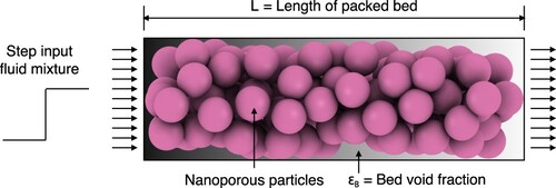
Figure 8. (Colour online) Different zones in a breakthrough curve at the exit of the fixed bed column. Fluid phase concentration of an adsorbing component as a function of time at the fixed bed column outlet. The profile is divided into three zones: (a) the unsaturated zone: where the maximum adsorption takes place, (b) mass transfer zone: where adsorption process progresses rapidly towards equilibrium, (c) saturated zone: where no more adsorption takes place as equilibrium between the fluid and the adsorbed phase is achieved.

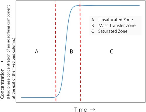
Molecules in the column can move in both axial and radial directions. In case of plug flow behaviour, any variation in the radial direction is absent so the velocity of the fluid, the concentration, and the porosity are assumed to be constant across any cross-section of the bed perpendicular to the axis of the bed. Variation of the velocity in the radial direction can be neglected if the flow is not highly viscous and no considerable boundary layer is formed in that direction. The assumption of neglecting radial gradients is widely accepted [135–137]. The effects of dispersion in all directions are included in the axial dispersion term [6]. To account for the adsorption, we use the Linear Driving Force (LDF) model [32]. In this model, the adsorption of molecules from all directions into adsorbent particles is lumped into a single entity, called average adsorbed loading $\left(q_i\right)$. One can also model the adsorption process by considering variation in the radial direction inside the zeolites. This is possible using the Fick diffusion model. Sircar and Hufton compared the LDF model with the rigorous Fick diffusion model [138]. These authors found that the details regarding the intra-pore diffusion are lost when breakthrough curves are modelled [138]. Therefore, the authors concluded that in most cases the LDF model is sufficient to account for the effects of adsorption.

Various mathematical models can be derived from conservation of mass, energy, and momentum and augmented by appropriate transport rate equations and equilibrium isotherms [139]. Mathematical models of fixed-bed columns for adsorption are reviewed by Tien [20,140], Worch [64,141], Siahpoosh et al. [142], Xu et al. [134], Shafeeyan et al. [137], Supian et al. [143], Unuabonah et al. [144], and many others. These models differ mainly in the form of the mass transfer rate, the form of the equilibrium isotherm, thermal effects, and the pressure drop along the bed. Fixed-bed column adsorption studies are reviewed by Patel [127] on removal of various contaminants from wastewater.

Fixed-bed models are either zero-phase, one-phase, two-phase or multi-phase resistance models [6,144]. A zero-phase model ignores mass transfer and assumes instantaneous equilibrium along the column. The one-phase resistance models assume local equilibrium in any cross section along the bed. These models take dispersion and/or diffusion into account but neglect intra-particle diffusion resistance and intra-particle axial dispersion. The one-phase models, known as chemical kinetic models, assume that the mass transfer rate is the difference between two opposing second-order reactions with different rate constants [145], and include [20,144]: the Thomas model [146], Bohart-Adams model [147], Yoon-Nelson models [148,149], and Clark model [150]. One-phase models have direct nonlinear mathematical expressions but are not very accurate in describing the breakthrough behaviour in a column [151]. Two-phase resistance models take into account both film and intra-particle diffusion. These models are more accurate than one-phase resistance models but have to be solved numerically. Multiphase resistance models take multiple types of diffusion (film diffusion, pore diffusion, and surface diffusion) into account. In the diffusion models, the particle is treated as a homogeneous phase [145]. Note that often surface reaction rates are assumed to be much faster than diffusion. Surface reactions should be considered when it affects the adsorption rate or is the controlling step. Plazinski et al. [152] reviewed sorption kinetic models including surface reaction mechanism. Medved and Cerny [153] reviewed surface diffusion of particles in porous media.

4.2. Theory

To model the fixed bed adsorber column, the following assumptions are considered [142]:

• The fixed bed is tubular and the adsorbent particles are spherical. The particles are packed uniformly into the fixed bed (no channeling occurs).

• No chemical reaction occurs in the column. This aspect will be considered in our future work.

• The fixed bed is initially filled with carrier gas.

• The gas phase behaves as an ideal gas mixture.

• The process is isothermal adsorption.

• The mass and velocity gradients are negligible in radial direction of the bed.

• The pressure gradient (if any) is invariant with time and column position and is not affected by the adsorption process.

• The fluid velocity is varying according to the total mass balance along the bed in multi-component systems. The fluid velocity will vary along the length of the column because of the variation in total pressure and/or adsorption of the molecules from the fluid phase.

• The axial dispersion is considered in the bulk phase.

• The carrier gas does not adsorb.

• The physical properties of the gas phase (axial dispersion coefficient and mass transfer coefficient) are those of the feed gas. These properties along with the properties (particle density and bed porosity) of the adsorbent are constant throughout the column.

For future versions of RUPTURA, we envision to include non-ideal gas behaviour, liquid phase conditions, non-isothermal breakthroughs, and chemical reactions.

We follow Worch [64] to outline the establishment of the material balance. Considering a differential volume element $\mathrm{d}V=A_{{}_R}\mathrm{d}z$, it can be assumed that the amount of adsorbate that is adsorbed onto the adsorbent or accumulated in the void fraction of the volume element must equal the difference between the input and the output of the volume element. Input and output occurs by advection and axial dispersion. The general mass balance equation is as follows [64] (202) ${\dot{N}}_{\mathrm{a}\mathrm{c}\mathrm{c}\mathrm{u}.}+{\dot{N}}_{\mathrm{a}\mathrm{d}\mathrm{s}.}={\dot{N}}_{\mathrm{a}\mathrm{d}\mathrm{v}.}+{\dot{N}}_{\mathrm{d}\mathrm{i}\mathrm{s}\mathrm{p}.}$(202) where $\dot{N}$ represents the change of the amount of adsorbate with time, and the indices indicate the processes accumulation, adsorption, advection, and dispersion.

• The accumulation term is: (203) ${\dot{N}}_{\mathrm{a}\mathrm{c}\mathrm{c}\mathrm{u}}={ϵ}_{{}_B}\mathrm{d}V\frac{\mathrm{\partial }c(t,z)}{\mathrm{\partial }t}$(203) where c represents the adsorbate concentration in the fluid phase, z is the distance along the bed length, t denotes time, and ${ϵ}_{{}_B}$ is the bed void fraction.

• The adsorption term is expressed as: (204) ${\dot{N}}_{\mathrm{a}\mathrm{d}\mathrm{s}}={\rho }_{{}_B}\mathrm{d}V\frac{\mathrm{\partial }\overline{q}(t,z)}{\mathrm{\partial }t}$(204) (205) $=(1-{ϵ}_{{}_B}){\rho }_{{}_P}\frac{\mathrm{\partial }\overline{q}(t,z)}{\mathrm{\partial }t}$(205) where ${\rho }_{{}_B}$ is the bed density, ${\rho }_{{}_P}$ is the particle density. The units of both ${\rho }_{{}_B}$ and ${\rho }_{{}_P}$ are $\left[\mathrm{k}\mathrm{g}/{\mathrm{m}}^3\right]$. $\overline{q}$ denotes the average concentration in adsorbent particle in $\left[\mathrm{m}\mathrm{o}\mathrm{l}/\left(\mathrm{k}\mathrm{g}\mathrm{f}\mathrm{r}\mathrm{a}\mathrm{m}\mathrm{e}\mathrm{w}\mathrm{o}\mathrm{r}\mathrm{k}\right)\right]$, which forms a link between the fluid and solid phase mass balance equations.

• Advection is the transport of substances due to the bulk motion of the fluid in the axial direction and is the difference between the input and output amount per unit time. (206) ${\dot{N}}_{\mathrm{a}\mathrm{d}\mathrm{v}}=u(t,z)A_{{}_R}c(t,z)-u(t,z+\mathrm{d}z)A_{{}_R}c(t,z+\mathrm{d}z)$(206) (207) $=-A_{{}_R}\frac{\mathrm{\partial }u(t,z)c(t,z)}{\mathrm{\partial }z}dz$(207) (208) $=-\mathrm{d}V\frac{\mathrm{\partial }u(t,z)c(t,z)}{\mathrm{\partial }z}$(208) (209) $=-{ϵ}_{{}_B}\mathrm{d}V\frac{\mathrm{\partial }v(t,z)c(t,z)}{\mathrm{\partial }z}$(209) where v is the interstitial velocity of the gas phase (related to the superficial gas velocity u by $v=u/{ϵ}_{{}_B}$).

• Assuming that the axial dispersion can be described by Fick's first law [154], the difference between input and output caused by dispersion is as follows: (210) ${\dot{N}}_{\mathrm{d}\mathrm{i}\mathrm{s}\mathrm{p}}=\mathcal{D}{ϵ}_{{}_B}{A}_{{}_R}{\left[\frac{\mathrm{\partial }c(t,z)}{\mathrm{\partial }z}\right]}_{z+\mathrm{d}z}-\mathcal{D}{ϵ}_{{}_B}{A}_{{}_R}{\left[\frac{\mathrm{\partial }c(t,z)}{\mathrm{\partial }z}\right]}_z$(210) (211) $=\mathcal{D}{ϵ}_{{}_B}{A}_R\frac{\mathrm{\partial }{c}^2(t,z)}{\mathrm{\partial }{z}^2}\mathrm{d}z$(211) (212) $=\mathcal{D}{ϵ}_{{}_B}\mathrm{d}V\frac{\mathrm{\partial }{c}^2(t,z)}{\mathrm{\partial }{z}^2}$(212) where $\mathcal{D}$ is the axial dispersion coefficient.

Introducing Equations (203(203) ${\dot{N}}_{\mathrm{a}\mathrm{c}\mathrm{c}\mathrm{u}}={ϵ}_{{}_B}\mathrm{d}V\frac{\mathrm{\partial }c(t,z)}{\mathrm{\partial }t}$(203) ), (205(205) $=(1-{ϵ}_{{}_B}){\rho }_{{}_P}\frac{\mathrm{\partial }\overline{q}(t,z)}{\mathrm{\partial }t}$(205) ), (209(209) $=-{ϵ}_{{}_B}\mathrm{d}V\frac{\mathrm{\partial }v(t,z)c(t,z)}{\mathrm{\partial }z}$(209) ), and (212(212) $=\mathcal{D}{ϵ}_{{}_B}\mathrm{d}V\frac{\mathrm{\partial }{c}^2(t,z)}{\mathrm{\partial }{z}^2}$(212) ) into Equation (202(202) ${\dot{N}}_{\mathrm{a}\mathrm{c}\mathrm{c}\mathrm{u}.}+{\dot{N}}_{\mathrm{a}\mathrm{d}\mathrm{s}.}={\dot{N}}_{\mathrm{a}\mathrm{d}\mathrm{v}.}+{\dot{N}}_{\mathrm{d}\mathrm{i}\mathrm{s}\mathrm{p}.}$(202) ), dividing by the control volume $\left(\mathrm{d}V\right)$ and the bed void-fraction $\left({ϵ}_{{}_B}\right)$, and applying the balance equation to each component, we obtain the main governing equation for the fixed-bed model [6,145]. (213) $\frac{\mathrm{\partial }{c}_i(t,z)}{\mathrm{\partial }t}=-\frac{\mathrm{\partial }\left(v(t,z)c_i(t,z)\right)}{\mathrm{\partial }z}+{\mathcal{D}}_i\frac{{\mathrm{\partial }}^2{c}_i(t,z)}{\mathrm{\partial }{z}^2}-\frac{1-{ϵ}_{{}_B}}{{ϵ}_{{}_B}}{\rho }_{{}_P}\frac{\mathrm{\partial }{\overline{q}}_i(t,z)}{\mathrm{\partial }t}$(213) For the ith component, the component mass balance including axial dispersion term, an advection flow term, accumulation in the fluid phase, and source term caused by the adsorption process on the adsorbent particles. If the system is non-isothermal, an additional heat-balance is required [6].

4.3. Axial dispersion

Models that consider the dispersion are referred to as dispersed-flow models, whereas models that neglect dispersion are termed plug-flow models. In practice, most experiments are set up such that the plug flow assumption is valid. During the fluid flow through the packed bed, axial mixing takes place, which reduces the efficiency of the separation process by broadening the mass transfer zone. Axial mixing is caused by molecular diffusion, turbulent mixing, flow splitting, and rejoining around particles, Taylor dispersion, channeling, and wall effects [6,155]. These phenomena can be minimised by choosing proper bed and flow conditions. Axial dispersion does depend on the Reynolds number and therefore, changes along the column when appreciable amounts are adsorbed. In particular, the Peclet number describes axial dispersion. The effects of all mechanisms that contribute to axial mixing are lumped into a single effective axial dispersion coefficient, ${\mathcal{D}}_z$. Generally, the contribution from molecular diffusion and Eddy diffusion or turbulence is considered in the formulation of dispersion coefficient. Coupling theory is used to add the contribution of both the terms as shown in the equation stated below [156]. (214) ${\mathcal{D}}_z=\gamma D_m+\frac{\lambda d_{p}v}{1+C{D}_m/\left(d_{p}v\right)}$(214) When intra-particle mass-transfer is neglected (if the product of Reynolds number and Schmidt number, $(Re\cdot Sc)$ $\gg 1$, advection dominates diffusion), ${\mathcal{D}}_z$ can be estimated using Equation (214(214) ${\mathcal{D}}_z=\gamma D_m+\frac{\lambda d_{p}v}{1+C{D}_m/\left(d_{p}v\right)}$(214) ).

Table 7 shows various correlations to calculate axial dispersion coefficient, ${\mathcal{D}}_z$. ${\mathcal{D}}_z$ is a function of molecular diffusivity $\left(D_m\right)$, particle radius $\left(r_{{}_P}\right)$, fluid phase velocity (v) and bed porosity $\left({ϵ}_{{}_B}\right)$. The molecular diffusivity, $D_m$ used in the expression for axial dispersion coefficient can be calculated either using Molecular Dynamics [83,161,162] or the Chapman-Enskog theory [163,164]: (215) $D_m=\frac{A{T}^{\frac{3}{2}}}{p{\sigma }_{12}^2\mathrm{\Omega }}{(\frac{1}{M_1}+\frac{1}{M_2})}^{0.5}$(215) In Equation (215(215) $D_m=\frac{A{T}^{\frac{3}{2}}}{p{\sigma }_{12}^2\mathrm{\Omega }}{(\frac{1}{M_1}+\frac{1}{M_2})}^{0.5}$(215) ), A is an empirical constant of magnitude $1.859\cdot {10}^{-7}$. T is the temperature in $\left[\mathrm{K}\right]$ and p is the partial pressure of the molecule in $\left[\mathrm{a}\mathrm{t}\mathrm{m}\right]$. M is the molar mass in $\left[\mathrm{g}/\mathrm{m}\mathrm{o}\mathrm{l}\right]$. ${\sigma }_{12}$ is the average collision diameter between molecules 1 and 2 in [Å] and Ω is the temperature dependent collision integral. The expressions for ${\sigma }_{12}$ and Ω [142] are as follows. (216) ${\sigma }_{12}=\frac{1}{2}({\sigma }_1+{\sigma }_2)$(216) (217) $\mathrm{\Omega }={(44.54{\left(k_{{}_B}T/{ϵ}_{i,j}\right)}^{-4.909}+1.911{\left(k_{{}_B}T/{ϵ}_{i,j}\right)}^{-1.575})}^{0.1}$(217) ${\sigma }_{i,j}$ in Equation (216(216) ${\sigma }_{12}=\frac{1}{2}({\sigma }_1+{\sigma }_2)$(216) ), and ${ϵ}_{i,j}$ in Equation (217(217) $\mathrm{\Omega }={(44.54{\left(k_{{}_B}T/{ϵ}_{i,j}\right)}^{-4.909}+1.911{\left(k_{{}_B}T/{ϵ}_{i,j}\right)}^{-1.575})}^{0.1}$(217) ) are the effective Lennard-Jones parameters [165,166] for a mixture of molecules i and j. ${ϵ}_{i,j}$ is defined by $\sqrt{{ϵ}_i{ϵ}_j}$ and $k_{{}_B}$ is the Boltzmann constant. The expressions for the Lennard-Jones parameters for a molecule i can be estimated as follows. (218) ${\sigma }_i=0.841V_{\mathrm{c}}^{1/3}$(218) (219) ${ϵ}_i=0.75k_{{}_B}{T}_{\mathrm{c}}$(219) In Equations (218(218) ${\sigma }_i=0.841V_{\mathrm{c}}^{1/3}$(218) ) and (219(219) ${ϵ}_i=0.75k_{{}_B}{T}_{\mathrm{c}}$(219) ), $V_{\mathrm{c}}$ and $T_{\mathrm{c}}$ are the critical volume and critical temperature of the molecule i respectively [142]. $V_{\mathrm{c}}$ is in [ų] and $T_{\mathrm{c}}$ is in [K].

Table 7. Correlations for estimation of axial dispersion coefficient, ${\mathcal{D}}_z$ in fixed bed adsorbers.

Dispersion Model	Conditions	Authors
${\mathcal{D}}_z=\frac{2r_{{}_P}v{ϵ}_{{}_B}}{0.2+0.011{\mathrm{R}\mathrm{e}}^{0.48}}$	${10}^{-3}<\mathrm{R}\mathrm{e}<{10}^3$	Chung and Wen [157]
${\mathcal{D}}_z=0.7D_m+\frac{5r_{{}_P}v}{1+4.4D_m/\left(r_{{}_P}v\right)}$	valid for liquids	De Ligny [156]
${\mathcal{D}}_z=0.7D_m+\frac{2r_{{}_P}v{ϵ}_{{}_B}}{0.18+0.008{\mathrm{R}\mathrm{e}}^{0.59}/\left(r_{{}_P}v\right)}$	–	Rastegar and Gu [158]
${\mathcal{D}}_z=0.73D_m+\frac{0.5d_{\mathrm{p}}v{ϵ}_{{}_B}}{1+\left(9.7D_m\right)/\left(v{ϵ}_{{}_B}{d}_{{}_P}\right)}$	$0.008<\mathrm{R}\mathrm{e}<50,0.0377<d_p<0.60\mathrm{c}\mathrm{m}$	Edwards and Richardson [159]
${\mathcal{D}}_z=\frac{20D_m}{{ϵ}_{{}_B}}+\frac{0.5D_{m}ScRe}{{ϵ}_{{}_B}}$	–	Shafeeyan, da Silva [137,160]
${\mathcal{D}}_z=(0.45+0.55{ϵ}_{{}_B})D_m+r_{{}_P}v$	–	Ruthven [6]

Notes: $D_m$ is the molecular diffusivity, Sc is the Schmidt number and Re is the Reynolds number. $r_{{}_P}$ and $d_{{}_P}$ are the particle radius and particle diameter respectively. v represents velocity and ${ϵ}_{{}_B}$ is the bed porosity.

4.4. Mass transfer models

Inside nanoporous materials, molecules can diffuse into the framework via pore diffusion and surface diffusion [24]. Diffusion of the particles in the pores occurs through two transfer processes depending on the pore size [6]: (1) molecular diffusion, which results from collisions between molecules, dominates in macro pores, (2) Knudsen diffusion occurs for smaller pore sizes due to collisions between molecules and the pore wall. In the surface diffusion mechanism, molecules hop between adsorption sites. It is therefore strongly dependent on concentration. For much more details on diffusion in nanoporous materials, see Ref. [167] and references therein.

The term $\mathrm{\partial }\overline{q}(t,z)/\mathrm{\partial }t$ in Equation (213(213) $\frac{\mathrm{\partial }{c}_i(t,z)}{\mathrm{\partial }t}=-\frac{\mathrm{\partial }\left(v(t,z)c_i(t,z)\right)}{\mathrm{\partial }z}+{\mathcal{D}}_i\frac{{\mathrm{\partial }}^2{c}_i(t,z)}{\mathrm{\partial }{z}^2}-\frac{1-{ϵ}_{{}_B}}{{ϵ}_{{}_B}}{\rho }_{{}_P}\frac{\mathrm{\partial }{\overline{q}}_i(t,z)}{\mathrm{\partial }t}$(213) ) describes adsorption and the overall rate of mass transfer from the fluid phase to the solid phase at time t and column distance z. The adsorbate molecules initially must cross the external film surrounding each adsorbent particle and then diffuse through and along the porous structure of the adsorbent. Many models are developed that differ in the rate-limiting mass transport step [134,144,168,169]: the Linear Driving Force (LDF) model [32], the homogeneous surface diffusion model [170], the film-solid diffusion model with a constant diffusivity [171], the branched pore kinetic-model [172], the pore diffusion model [6,173], the film-pore diffusion model [174], the diffusion flow-film particle diffusion model [175], the diffusion flow-local equilibrium model [176], the film pore and surface diffusion model [177–180], and the concentration-dependent surface diffusivity model [181] to name but a few. The most frequently applied approximate rate law to simplify the calculation is the LDF approximation [32]. In most cases, the LDF model is a good approximation to the exact but much more complicated surface and pore diffusion models [64].

Self-diffusion is a measure of the mobility of molecules due to their thermal motions, while collective diffusion is a dynamic process, involving many particles, due to their cooperative movements [182]. The collective diffusion is related to the transport diffusion coefficient by the thermodynamic factor [183–185], which can be obtained from the adsorption isotherms. Transport diffusion, taking the thermodynamic effects into account using a Fickian type of approach, can be incorporated in the equipment design equations. The differences between collective and transport diffusion show that there are different viewpoints possible to study diffusion [184–186]:

• In the Fick approach, the fluxes $\mathbf{N}$ are taken to be linearly dependent on the gradients of the loadings $\mathrm{\nabla }{c}_i$ of all species with the ‘constants’ of proportionality being the Fick diffusivity matrix.

• In the Onsager approach, the fluxes are postulated as linear functions of the chemical potential gradients ($\mathrm{\nabla }{\mu }_i$), with the proportionality constants being the Onsager coefficients $L_{ij}$.

• The Maxwell-Stefan formulation balances diffusive and drag forces, while Fick and Onsager postulate phenomenological flux expressions. The Maxwell-Stefan diffusivity can be related to Fick diffusivity as follows [183,187] (220) $D_{{}_F}=D_{{}_{MS}}\mathrm{\Gamma }$(220) In Equation (220(220) $D_{{}_F}=D_{{}_{MS}}\mathrm{\Gamma }$(220) ), $D_{{}_{MS}}$ is the Maxwell-Stefan diffusivity and $D_{{}_F}$ is the Fick diffusivity. Γ is the thermodynamic correction factor which is derived using chemical potential as the driving force [187]. This factor can be determined from adsorption isotherms after differentiation as shown below [187]. (221) $\mathrm{\Gamma }\equiv \frac{\mathrm{\partial }\ln f}{\mathrm{\partial }\ln q}$(221) In Equation (221(221) $\mathrm{\Gamma }\equiv \frac{\mathrm{\partial }\ln f}{\mathrm{\partial }\ln q}$(221) ), f is the fugacity and q is the adsorbed loading. To understand the underlying principles behind the diffusion process, it is more convenient to describe this phenomenon using Maxwell-Stefan diffusivity [187]. This approach clearly distinguishes between self diffusivity, diffusivity of a species inside an adsorbent, and diffusivity describing interaction between different species [187].

The viewpoints differ in how to set up the flux-driving force relationship for transport diffusion in nanoporous materials under non-equilibrium conditions [184,188–190].

In Onsager linear theory, the driving force of diffusion is the gradient of the chemical potential, μ, of the adsorbed particles. The diffusion flux $\mathbf{J}$ is [191] (222) $\mathbf{J}=-L\mathrm{\nabla }\left(\frac{\mu }{T}\right)=-\frac{L}{T}\frac{\mathrm{\partial }\mu }{\mathrm{\partial }q}\mathrm{\nabla }q$(222) where L is the Onsager coefficient and q is the adsorption loading. From the practical point of view, the flux $\mathbf{J}$ is usually related to the gradient diffusion coefficient D that depends on adsorption [191] (223) $\mathbf{J}=-D\mathrm{\nabla }q,D=D_0\frac{1}{k_{B}T}\frac{\mathrm{\partial }\mu }{\mathrm{\partial }\ln q}$(223) where $D_0=kL/q$ does not depend on adsorption and has the meaning of the diffusivity at zero loading. The driving force for diffusion is more correctly expressed in terms of chemical potentials, but Fick's law provides a qualitatively and quantitatively correct representation of adsorption systems as long as the diffusivity is allowed to be a function of the adsorbate concentration [192]. However, for convenience, the diffusivity is often taken as the self-diffusivity and assumed to be a constant. In the limit of zero loading, the self-, collective-, and transport diffusivities become equal.

Film diffusion comprises the transport of the adsorbate from the bulk fluid to the external surface of the adsorbent particle. As long as the state of equilibrium is not reached, the concentration at the external adsorbent surface is always lower than in the bulk fluid due to the continuing adsorption process. As a consequence, a concentration gradient results that extends over a boundary layer of thickness δ (schematically shown in Figure 9). The difference between the concentration in the bulk solution, c, and the concentration at the external surface, $c_s$, acts as a driving force for the mass transfer through the boundary layer. The mass transfer flux ${\dot{n}}_F$ for the film diffusion can be derived from Fick's law (224) ${\dot{n}}_{{}_F}=D_L\frac{\mathrm{d}c}{\mathrm{d}\delta }$(224) leading to a film mass transfer equation [64] (225) $\frac{\mathrm{d}\overline{q}}{\mathrm{d}t}=k_F\frac{a_{{}_{VR}}}{{\rho }_{{}_B}}(c-c_{{}_S})$(225) where $k_F$ is the film mass transfer coefficient in $\left[{\mathrm{m}\mathrm{s}}^{-1}\right]$, $c_{{}_S}$ the concentration at the external surface, and the external surface related to the column $\left(a_{VR}\right)$ is (226) $a_{{}_{VR}}=A_{{}_S}/V_{{}_B}$(226) where $A_{{}_S}$ is the external adsorbent surface area and $V_{{}_B}$ is the fixed-bed volume. For spherical particles, $a_{{}_{VR}}=(1-{ϵ}_{{}_B})3/r_{{}_P}$. In most practical cases, the film diffusion influences only at the beginning of the adsorption process. At later stages of the process, the intra-particle diffusion becomes more important.

Figure 9. (Colour online) Loading and concentration profiles according to the pore diffusion model with external mass transfer resistance. The external mass transfer resistance is modeled using the film flux ${\dot{n}}_F\left(t\right)=K_{{}_F}\left(c\right(t)-c_{{}_S}(t\left)\right)$, which is the linear difference of the concentration $c\left(t\right)$ in the bulk solution, and the concentration $c_s\left(t\right)$ at the surface of the crystallite. The flux ${\dot{n}}_T={\dot{n}}_{{}_P}+{\dot{n}}_{{}_S}$ is the sum of the pore diffusion and surface diffusion: ${\dot{n}}_T=D_{{}_P}\mathrm{\partial }{c}_p/\mathrm{\partial }r+{\rho }_{{}_P}{D}_{{}_S}\mathrm{\partial }q/\mathrm{\partial }r$. The continuity of the materials fluxes requires ${\dot{n}}_F={\dot{n}}_{{}_T}$. The surface is considered to be in equilibrium and the adsorbent loading $q(r_p,t)=q\left(p\right(t\left)\right)$ is calculated from the isotherm with functional form q, where the pressure p is related to the surface concentration $c_{{}_S}$ via the ideal gas law as $p=RT{c}_{{}_S}$.

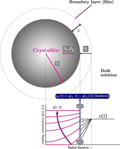
Figure 10. (Colour online) Loading and concentration profiles according to the Linear Driving Force (LDF) model with external mass transfer resistance. The LDF model assumes that there is linear gradient within the solution-side film and within a comparable fictive solid film. The film flux ${\dot{n}}_F\left(t\right)=K_{{}_F}\left(c\right(t)-c_{{}_S}(t\left)\right)$ is the linear difference of the concentration $c\left(t\right)$ in the bulk solution, and the concentration $c_{{}_S}\left(t\right)$ at the surface of the crystallite. The solid flux ${\dot{n}}_{{}_S}$ is the linear difference between the equilibrium loading $q_{{}_S}$ at the surface and the average loading $\overline{q}$: ${\dot{n}}_{{}_S}\left(t\right)={\rho }_{{}_P}{k}_{{}_S}\left(q_{{}_S}\right(t)-\overline{q}(t\left)\right)$, where ${\rho }_{{}_P}$ is the particle density, $k_{{}_S}$ is the intra-particle mass transfer coefficient. The continuity of the materials fluxes requires ${\dot{n}}_{{}_F}={\dot{n}}_{{}_S}$. The surface is considered to be in equilibrium and the adsorbent loading $q(r_{{}_P},t)=q\left(p\right(t\left)\right)$ is calculated from the isotherm with functional form q, where the pressure p is related to the surface concentration $c_{{}_S}$ via the ideal gas law as $p=RT{c}_{{}_S}$.

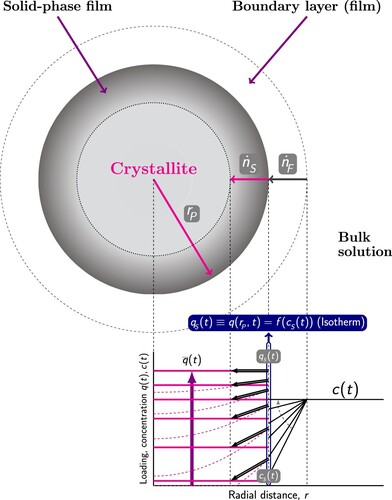
The local equilibrium model ignores the mass transfer resistance, and assumes that the mass transfer between solid adsorbent particles and external gas is instantaneous. (227) $\frac{\mathrm{\partial }{q}_i}{\mathrm{\partial }t}=\frac{\mathrm{\partial }{q}_i^{\ast }}{\mathrm{\partial }t}$(227) where $q_i$ is the average amount of component i adsorbed, $q_i^{\ast }$ is the amount adsorbed at equilibrium given by the selected adsorption isotherm model. Because of neglecting the mass transfer resistance, the model has accepted limitation in the practical applications.

In the Homogeneous Surface Diffusion Model (HSDM) [170,193], the main diffusion mechanism is the surface diffusion. The HSDM assumptions are the following [194]:

• mass balance around a spherical shell element.

• internal mass transfer is only governed by surface diffusion.

• external mass transfer is governed by a linear driving force.

• at the solid/fluid interface, there is continuity between external mass transfer and internal diffusion.

• at the solid/fluid interface, there is equilibrium between adsorbate concentration in the fluid and adsorbate load on the surface.

• the adsorbent particle is assumed to be spherical and homogeneous.

The adsorbent is assumed to be a uniform medium in which the solute adsorbs on the surface and diffuses inwards with an effective diffusivity in accordance with Fick's law. For surface diffusion, the mass transfer rate per unit of surface area, ${\dot{n}}_{{}_S}$, is obtained using Fick's law as (228) ${\dot{n}}_{{}_S}={\rho }_{{}_P}{D}_{{}_S}\frac{\mathrm{\partial }q}{\mathrm{\partial }r}$(228) where $D_{{}_S}$ is the surface diffusion coefficient and r is the radial coordinate. Imposing a material balance and assuming $D_s$ to be constant leads to the basic mathematical form of the HSDM for a spherical particle [64,140,195]: (229) $\frac{\mathrm{\partial }q}{\mathrm{\partial }t}=\frac{D_{{}_S}}{r^2}\frac{\mathrm{\partial }}{\mathrm{\partial }r}\left(r^2\frac{\mathrm{\partial }q}{\mathrm{\partial }r}\right)=D_{{}_S}(\frac{{\mathrm{\partial }}^{2}q}{\mathrm{\partial }{r}^2}+\frac{2}{r}\frac{\mathrm{\partial }q}{\mathrm{\partial }r})$(229) The homogeneous surface diffusion model is closely related to the homogeneous solid diffusion model and the film-solid diffusion model [196]. In the homogeneous solid diffusion model, all solute within the particle, whether it is in pore fluid or adsorbed by particle skeleton is lumped into a single quantity, q [195].

In the Pore Diffusion Model (PDM) [6], the adsorbate transport within the adsorbent particles takes place in the pore fluid, instead of on the surface. For pore diffusion, the mass transfer rate per unit of surface area, ${\dot{n}}_s$, is again obtained using Fick's law as (230) ${\dot{n}}_{{}_P}=D_{{}_P}\frac{\mathrm{\partial }{c}_{{}_P}}{\mathrm{\partial }r}$(230) where $D_{{}_P}$ is the pore diffusion coefficient and r is the radial coordinate. In the surface diffusion model, the adsorbent is considered to be homogeneous, and the adsorption equilibrium is assumed to exist only at the outer surface of the adsorbent particle. In the case of pore diffusion, however, the adsorption equilibrium has to be considered at each point of the pore system. In general, it is assumed that there is a local equilibrium between the pore fluid concentration and the solid-phase concentration. Imposing a material balance leads to a more complicated description [64,195] (231) ${\rho }_{{}_P}\frac{\mathrm{\partial }q}{\mathrm{\partial }t}+{ϵ}_{{}_P}\frac{\mathrm{\partial }{c}_{{}_P}}{\mathrm{\partial }t}=D_{{}_P}(\frac{{\mathrm{\partial }}^2{c}_{{}_P}}{\mathrm{\partial }{r}^2}+\frac{2}{r}\frac{\mathrm{\partial }{c}_{{}_P}}{\mathrm{\partial }r})$(231) In the Pore and Surface Diffusion Model (PSDM) [177], the adsorbate transport within the adsorbent particles takes place via surface and pore diffusion. The total flux is then given as the sum of the fluxes caused by surface diffusion and by pore diffusion [64,195] (232) ${\dot{n}}_{{}_T}={\dot{n}}_S+{\dot{n}}_{{}_P}={\rho }_{{}_P}{D}_{{}_S}\frac{\mathrm{\partial }q}{\mathrm{\partial }r}+D_{{}_P}\frac{\mathrm{\partial }{c}_{{}_P}}{\mathrm{\partial }r}$(232) (233) $\frac{\mathrm{\partial }q}{\mathrm{\partial }t}=D_{{}_S}(\frac{{\mathrm{\partial }}^{2}q}{\mathrm{\partial }{r}^2}+\frac{2}{r}\frac{\mathrm{\partial }q}{\mathrm{\partial }r})+\frac{D_{{}_P}}{{\rho }_{{}_P}}(\frac{{\mathrm{\partial }}^2{c}_{{}_P}}{\mathrm{\partial }{r}^2}+\frac{2}{r}\frac{\mathrm{\partial }{c}_{{}_P}}{\mathrm{\partial }r})$(233) The concentration profiles for film and pore/surface diffusion are schematically shown in Figure 9.

The intra-particle diffusion models discussed so far include partial derivatives with respect to time and radial coordinate, which causes an increased effort for the numerical solution. The Linear Driving Force (LDF) model states that the rate of adsorption is proportional to the amount of adsorbate still required to achieve equilibrium [195]. The equation for the flux is approximated by (234) ${\dot{n}}_{{}_S}={\rho }_{{}_P}k(q_{{}_S}-\overline{q})$(234) where ${\rho }_{{}_P}$ is the particle density, k is the mass transfer coefficient, $q_{{}_S}$ is the adsorbent loading at the external surface of the adsorbent (which is a function of the bulk composition), and $\overline{q}$ is the mean loading in the particle. The following mass transfer equation can be derived (235) $\frac{\mathrm{d}\overline{q}}{\mathrm{d}t}=k(q_{{}_S}-\overline{q})$(235) The uptake rate of a species into adsorbent particles is proportional to the linear difference between the concentration of that species at the outer surface of the particle $q_{{}_S}$ (equilibrium adsorption amount) and its average concentration within the particle $\overline{q}$. $r_{{}_P}$ is the crystallite particle radius.

The LDF model can be derived from a model with a concentration profile within the particle. Assuming a quadratic concentration profile leads directly to the LDF form [197]. Glueckauf [32] derived a general expression to account for the mass transfer of the molecules from the fluid phase into the adsorbent [197]. This expression is valid for arbitrary variation of surface concentration of the adsorbates inside the solid particles [32]. Glueckauf also showed that for larger values of the product of mass transfer coefficient (k) and time (t), the expression is identical to the LDF model [32]. The volume-averaged adsorption amount $\overline{q}$ is given by (236) $\overline{q}\left(t\right)=\frac{{\int }_0^{r_{{}_P}}q(r,t)4\pi r^2\mathrm{d}r}{\frac{4}{3}\pi r_{{}_P}^3}=\frac{3}{r_{{}_P}^3}{\int }_0^{r_{{}_P}}q(r,t)r^2\mathrm{d}r$(236) Taking the derivative we get (237) $\frac{\mathrm{\partial }\overline{q}}{\mathrm{\partial }t}=\frac{3}{r_{{}_P}}{\int }_0^{r_{{}_P}}\frac{\mathrm{\partial }q}{\mathrm{\partial }t}{r}^2\mathrm{d}r$(237) Substituting the diffusion equation for spherical geometry [170,177] (238) $\frac{\mathrm{\partial }q(r,t)}{\mathrm{\partial }t}=D{\mathrm{\nabla }}^{2}q(r,t)=\frac{D}{r^2}\frac{\mathrm{\partial }}{\mathrm{\partial }r}\left[r^2\frac{\mathrm{\partial }q}{\mathrm{\partial }t}\right]$(238) into this equation we get (239) $\frac{\mathrm{\partial }\overline{q}}{\mathrm{\partial }t}=\frac{3D}{r_{{}_P}}{\int }_0^{r_{{}_P}}\frac{\mathrm{\partial }}{\mathrm{\partial }r}\left(r^2\frac{\mathrm{\partial }q}{\mathrm{\partial }r}\right)\mathrm{d}r=\frac{3D}{r_{{}_P}}{\left[\frac{\mathrm{\partial }q}{\mathrm{\partial }r}\right]}_{r=r_{{}_P}}$(239) In Equations (238(238) $\frac{\mathrm{\partial }q(r,t)}{\mathrm{\partial }t}=D{\mathrm{\nabla }}^{2}q(r,t)=\frac{D}{r^2}\frac{\mathrm{\partial }}{\mathrm{\partial }r}\left[r^2\frac{\mathrm{\partial }q}{\mathrm{\partial }t}\right]$(238) ) and (239(239) $\frac{\mathrm{\partial }\overline{q}}{\mathrm{\partial }t}=\frac{3D}{r_{{}_P}}{\int }_0^{r_{{}_P}}\frac{\mathrm{\partial }}{\mathrm{\partial }r}\left(r^2\frac{\mathrm{\partial }q}{\mathrm{\partial }r}\right)\mathrm{d}r=\frac{3D}{r_{{}_P}}{\left[\frac{\mathrm{\partial }q}{\mathrm{\partial }r}\right]}_{r=r_{{}_P}}$(239) ), D is the Fickian diffusivity. Next, we consider a generalised concentration profile (240) $q(t,r)=A\left(t\right)+B\left(t\right)r^n$(240) The linear term has been left out on account of spherical symmetry [197]. $A\left(t\right)$ and $B\left(t\right)$ can be solved from the two boundary conditions (241) ${\left(\frac{\mathrm{\partial }q}{\mathrm{\partial }r}\right)}_{r=0}=0$(241) (242) $q(r=r_{{}_P})=q(t,r_{{}_P})$(242) A general solution for the concentration profiles is (243) $q(t,r)=\{\begin{array}{l}q(t,r_{{}_P})-\frac{n+3}{n}[q(t,r_{{}_P})-\overline{q}]\\ +\frac{n+3}{n}\frac{1}{r_{{}_P}^n}[q(t,r_{{}_P})-\overline{q}]r^{n}0\le r\le r_{{}_P}\\ q(t,r_{{}_P})r=r_{{}_P}\end{array}$(243) Taking the derivative of the concentration profiles (244) ${\left[\frac{\mathrm{\partial }q}{\mathrm{\partial }r}\right]}_{r=r_{{}_P}}=\frac{n+3}{r_{{}_P}}[q(t,r_{{}_P})-\overline{q}]$(244) Finally, substituting the result for n = 2 into Equation (239(239) $\frac{\mathrm{\partial }\overline{q}}{\mathrm{\partial }t}=\frac{3D}{r_{{}_P}}{\int }_0^{r_{{}_P}}\frac{\mathrm{\partial }}{\mathrm{\partial }r}\left(r^2\frac{\mathrm{\partial }q}{\mathrm{\partial }r}\right)\mathrm{d}r=\frac{3D}{r_{{}_P}}{\left[\frac{\mathrm{\partial }q}{\mathrm{\partial }r}\right]}_{r=r_{{}_P}}$(239) ) leads to the LDF equation (245) $\frac{\mathrm{\partial }\overline{q}}{\mathrm{\partial }t}=\frac{15D}{r_{{}_P}^2}(q_{{}_S}-\overline{q})$(245) Therefore, the LDF model can be deduced from assuming a quadratic concentration profile [195,197]. The precision of the LDF models can be improved by using higher order models [198]. The LDF concentration profiles are schematic shown in Figure 10.

Although the LDF model was originally developed as a simplified version of the surface diffusion model [64], it can also be related to the pore diffusion model. As shown for the combined surface and pore diffusion mechanism, an effective surface diffusion coefficient can be defined as (246) $D_{{}_S}=D_{{}_S}+\frac{D_{{}_P}}{{\rho }_{{}_P}}\frac{\mathrm{\partial }{c}_{{}_P}}{\mathrm{\partial }q}\approx D_{{}_S}+\frac{D_{{}_P}}{{\rho }_{{}_P}}\frac{c_0}{q_0}$(246) In Equation (246(246) $D_{{}_S}=D_{{}_S}+\frac{D_{{}_P}}{{\rho }_{{}_P}}\frac{\mathrm{\partial }{c}_{{}_P}}{\mathrm{\partial }q}\approx D_{{}_S}+\frac{D_{{}_P}}{{\rho }_{{}_P}}\frac{c_0}{q_0}$(246) ), $c_0$ and $q_0$ represent initial (t = 0) fluid phase concentration and adsorbed loading of the component. It is also possible to link the mass transfer coefficient $\left(k_{{}_S}\right)$ used in the LDF model with the effective surface diffusion coefficient $\left(D_{{}_S}\right)$ by [197] (247) $k_{{}_S}=\frac{15D^{\mathrm{e}\mathrm{f}\mathrm{f}}}{r_{{}_P}^2}=\frac{15D_{{}_S}}{r_{{}_P}^2}+\frac{15D_{{}_P}}{r_{{}_P}^2}\frac{c_0}{{\rho }_{{}_P}{q}_0}$(247) Surface diffusion as well as pore diffusion can be approximated by the LDF model. In fact, the LDF model can be viewed as a diffusion model where the overall kinetic constant in Equation (235(235) $\frac{\mathrm{d}\overline{q}}{\mathrm{d}t}=k(q_{{}_S}-\overline{q})$(235) ) is a combination of all types of diffusivities such as the film diffusivity and the intra-particle pore and surface diffusivities. The LDF model can also be extended to include coupled diffusion effects by using the Maxwell-Stefan diffusion formulation [199]. This model reduces the computational time significantly and is the most widely used model to describe the mass transfer kinetics. We have also incorporated this model in our code to account for the mass transfer kinetics. The LDF model includes competitive adsorption processes by combining it with a mixture adsorption prediction model that determines the relation between the concentrations and adsorbed amounts at the external surface.

4.5. Mixture loading prediction

In the multi-component breakthrough computation, the loading $q_i$ of species i depends on the concentrations $c_i$ of all N species (248) $q_i=q(c_1,c_2,\dots ,c_{N_{{}_C}})$(248) This would require mixture isotherms over all possible ranges of mole fraction. The equilibrium loadings $q_i$ for the components in the mixture are therefore computed from mixture prediction models like IAST using single-component adsorption isotherms. The total average molar loadings of the mixture $\left({\overline{q}}_{{}_T}\right)$ within the crystallite is obtained by a summation over all $N_{{}_C}$ components. (249) ${\overline{q}}_{{}_T}(t,z)=\sum _{i=1}^{N_{{}_C}}{\overline{q}}_i(t,z).$(249) There are three possibilities to couple IAST equations in adsorptive bed dynamics [73]:

(1)	The reduced grand potential can be treated as a dependent variable of time and space and added to the system of differential equations, describing the bed dynamics [200].
(2)	Computation of the adsorption equilibrium separately at each time step.
(3)	A B-spline approach to pre-compute the equilibrium states [116]. B-splines are also known as the basis splines. These are constructed using polynomial functions joined at nodes. For a set of knots or nodes, ${\lambda }_j$, with j = 0 to g + 1, g−k independent B-splines can be constructed. The summation of such independent splines leads to a spline function. Equilibrium loadings are calculated using IAST for the first time and then the coefficients involved in the B-spline functions are fitted to the data obtained. Further, interpolations are performed to calculate the equilibrium loadings. This helps in avoiding the iterative calculations involved in IAST when called inside the breakthrough code [116].

This first option results in a strongly non-linear system of differential-algebraic equations which is difficult to solve, computationally expensive and time consuming [73]. For more than two components, the B-spline approach results in additional multidimensional fitting issues, losing its advantages and limiting the applicability to the binary case [73]. The second option is computationally less expensive than the first one as the IAST equations are solved separately to the bed dynamics. Unlike the B-spline approach, this method does not have limitations regarding the number of components present in the system. These advantages make the second method a popular approach for calculating equilibrium loading in fixed bed adsorption problems [73]. Therefore, we have also adopted this approach in our code.

In this work, the IAST equations are solved using the FastIAS and the Nested-Loop bisection method. The latter has the advantage of calculating equilibrium loadings up to machine precision (ca. ${10}^{-15}$). A typical working precision considered by current IAST methods is ca. ${10}^{-8}$ [73]. Moreover, we have also incorporated the explicit isotherms mentioned in Section 3.4.5. These isotherms can account for the size-effects of the components on the adsorption behaviour. Originally, these equations were developed for adsorbents having single sites. We have extended this model to tackle multi sites adsorption [31]. We have used a segregated approach where the adsorbed phase is in equilibrium with the gas phase at each site. This method calculates equilibrium loadings with similar accuracy to the segregated IAST approach by Swisher et al [29]. The segregated approaches are useful in case of non-uniform adsorption surfaces, where IAST can be inadequate in calculating the correct equilibrium loadings [29].

The explicit isotherms do not require any iterations to calculate the loadings. For integration with the breakthrough model, this method makes the code about 3 times faster than using IAST [31]. Explicit isotherms are similar in speed as using FastIAS using caching, but are not iterative and hence always converging.

4.6. Existing breakthrough software

Different software is currently available for predicting breakthrough curves:

• Fixed-bed Adsorption Simulation Tool (FAST) [201]: It is a windows based software which is free of charge for academic or any other non-commercial purposes. It is licensed under a Creative Commons Attribution-Noncommercial-No Derivative Works 3.0 Unported License. FAST predicts the breakthrough curves for fixed bed type filters used in water treatment. The solid phase mass transfer can be modelled using a homogeneous surface diffusion model or LDF model.

• Multi-Flow Inversion of Tracer (MFIT) [202]: It is also a Windows based open-source software package for calculating breakthrough curves for tracer components present in ground water. This software is distributed under the Creative Commons Attribution 4.0 License.

• ProSim Dynamic Adsorption Column Simulation (ProSim DAC) [203]: It is a commercial software used for adsorption and regeneration steps in temperature swing adsorption (TSA), pressure swing adsorption (PSA), vacuum and temperature swing adsorption, etc. It finds its application in hydrogen refining, isotopic separation, emission control of volatile organic compounds and solvent recovery.

• 3P Sim [204]: It is a commercial software. 3P Sim is a part of the dynamic sorption analyser instrument, mixSorb L. It can calculate mixture isotherms from pure component isotherms and also evaluate breakthrough curves based on mass and energy balances.

• Aspen Adsorption [205]: Aspen Adsorption is a commercial flowsheet simulator. It is used to design, analysis, simulation, and optimisation of gas and liquid adsorption systems. It is used for both PSA and TSA processes.

Various commercial numerical platforms have been applied for the modeling of the PSA process [206], such as gPROMS [207], MATLAB [208] and FLUENT [209]. Many research groups have their own in-house breakthrough codes which are not released as open source codes. These include the work of Krishna and Baur [187], Rodriguez [19,160], Worch [64], Chung et al. [210], etc. Instead of the LDF model, Krishna and Baur solved a partial differential equation along the crystal diffusion path. The diffusive flux used in the model is provided by Maxwell-Stefan equations [187]. Maxwell-Stefan diffusivity formulation involves a thermodynamic correction factor and binary diffusivities correlating different species. These parameters are evaluated locally along the crystal diffusion path [187]. Chung et al. [210] used breakthrough curve modelling to screen nanoporous materials for hexane and heptane isomer separations. It is an isothermal model with LDF approximation for the mass transfer kinetics of the isomers and Darcy's equation [211] for the pressure drop along the length of the column.

4.7. Breakthrough model implementation

4.7.1. Model

The ideal gas law reads (250) $c_i=\frac{y_i{p}_{{}_T}}{RT}=\frac{p_i}{RT}$(250) where $y_i$ is the mole fraction of component i in the gas phase, $p_{{}_T}$ is the total pressure, $p_i$ is the partial pressure, T is the gas temperature, and R the universal gas constant. Assuming ideal gas behaviour for the gas phase and isothermal conditions, the partial pressures in the gas phase at position z and time t are obtained by solving the material balance for each component $i=1,\dots ,N_{{}_C}$ [6,145]. Here, the material balance shown in Equation (213(213) $\frac{\mathrm{\partial }{c}_i(t,z)}{\mathrm{\partial }t}=-\frac{\mathrm{\partial }\left(v(t,z)c_i(t,z)\right)}{\mathrm{\partial }z}+{\mathcal{D}}_i\frac{{\mathrm{\partial }}^2{c}_i(t,z)}{\mathrm{\partial }{z}^2}-\frac{1-{ϵ}_{{}_B}}{{ϵ}_{{}_B}}{\rho }_{{}_P}\frac{\mathrm{\partial }{\overline{q}}_i(t,z)}{\mathrm{\partial }t}$(213) ) is modified in terms of the partial pressures as shown below. (251) $\frac{1}{RT}\frac{\mathrm{\partial }{p}_i(t,z)}{\mathrm{\partial }t}=-\frac{1}{RT}\frac{\mathrm{\partial }\left(v(t,z)p_i(t,z)\right)}{\mathrm{\partial }z}+\frac{1}{RT}{\mathcal{D}}_i\frac{{\mathrm{\partial }}^2{p}_i(t,z)}{\mathrm{\partial }{z}^2}-\frac{1-{ϵ}_{{}_B}}{{ϵ}_{{}_B}}{\rho }_{{}_P}\frac{\mathrm{\partial }{\overline{q}}_i(t,z)}{\mathrm{\partial }t}$(251) Using the LDF approach yields (252) $\frac{\mathrm{\partial }{\overline{q}}_i(t,z)}{\mathrm{\partial }t}=k_i(q_{\mathrm{e}\mathrm{q},i}-{\overline{q}}_i)$(252) Because of adsorption and dispersion, the interstitial velocity v in fixed-bed adsorption is not constant. To calculate the velocity profile, the material balance for the overall mixture is considered by summing Equation (251(251) $\frac{1}{RT}\frac{\mathrm{\partial }{p}_i(t,z)}{\mathrm{\partial }t}=-\frac{1}{RT}\frac{\mathrm{\partial }\left(v(t,z)p_i(t,z)\right)}{\mathrm{\partial }z}+\frac{1}{RT}{\mathcal{D}}_i\frac{{\mathrm{\partial }}^2{p}_i(t,z)}{\mathrm{\partial }{z}^2}-\frac{1-{ϵ}_{{}_B}}{{ϵ}_{{}_B}}{\rho }_{{}_P}\frac{\mathrm{\partial }{\overline{q}}_i(t,z)}{\mathrm{\partial }t}$(251) ) over all components (253) $\frac{\mathrm{\partial }{p}_{{}_T}}{\mathrm{\partial }t}=-\frac{\mathrm{\partial }\left(v{p}_{{}_T}\right)}{\mathrm{\partial }z}+\sum _{i=1}^{N_{{}_C}}({\mathcal{D}}_i\frac{{\mathrm{\partial }}^2{p}_i}{\mathrm{\partial }{z}^2}-RT\frac{1-{ϵ}_{{}_B}}{{ϵ}_{{}_B}}{\rho }_{{}_P}{k}_i(q_{\mathrm{e}\mathrm{q},i}-{\overline{q}}_i))$(253) The total pressure along the column is invariant with time and has a constant gradient along the length of the column. Therefore, Equation (253(253) $\frac{\mathrm{\partial }{p}_{{}_T}}{\mathrm{\partial }t}=-\frac{\mathrm{\partial }\left(v{p}_{{}_T}\right)}{\mathrm{\partial }z}+\sum _{i=1}^{N_{{}_C}}({\mathcal{D}}_i\frac{{\mathrm{\partial }}^2{p}_i}{\mathrm{\partial }{z}^2}-RT\frac{1-{ϵ}_{{}_B}}{{ϵ}_{{}_B}}{\rho }_{{}_P}{k}_i(q_{\mathrm{e}\mathrm{q},i}-{\overline{q}}_i))$(253) ) is modified as shown below. (254) $p_{{}_T}\frac{\mathrm{\partial }v}{\mathrm{\partial }z}=\sum _{i=1}^{N_{{}_C}}({\mathcal{D}}_i\frac{{\mathrm{\partial }}^2{p}_i}{\mathrm{\partial }{z}^2}-RT\frac{1-{ϵ}_{{}_B}}{{ϵ}_{{}_B}}{\rho }_{{}_P}{k}_i(q_{\mathrm{e}\mathrm{q},i}-{\overline{q}}_i))-v\frac{\mathrm{\partial }{p}_{{}_T}}{\mathrm{\partial }z}$(254) The pressure gradient $(\mathrm{\partial }{p}_{{}_T}/\mathrm{\partial }z=\mathrm{c}\mathrm{o}\mathrm{n}\mathrm{s}\mathrm{t}\mathrm{a}\mathrm{n}\mathrm{t})$ can be calculated using the Ergun equation as shown below [212]. The Ergun equation considers both viscous and inertial effects. Apart from the Ergun equation, the Darcy [211], and Carman-Kozeny [213] equations could also be used but these equations are valid only for viscous flows. (255) $\frac{\mathrm{\Delta }P}{L}=\frac{150\mu L}{d_{{}_P}^2}\frac{{(1-{ϵ}_{{}_B})}^2}{{\left({ϵ}_{{}_B}\right)}^3}v+\frac{1.75L{\rho }_{{}_f}}{d_{{}_P}}\frac{(1-{ϵ}_{{}_B})}{{\left({ϵ}_{{}_B}\right)}^3}v\left|v\right|$(255) In Equation (255(255) $\frac{\mathrm{\Delta }P}{L}=\frac{150\mu L}{d_{{}_P}^2}\frac{{(1-{ϵ}_{{}_B})}^2}{{\left({ϵ}_{{}_B}\right)}^3}v+\frac{1.75L{\rho }_{{}_f}}{d_{{}_P}}\frac{(1-{ϵ}_{{}_B})}{{\left({ϵ}_{{}_B}\right)}^3}v\left|v\right|$(255) ), $\mathrm{\Delta }P/L$ is the pressure gradient inside the column of length L. μ is the dynamic viscosity in $\left[\mathrm{P}\mathrm{a}\mathrm{s}\right]$, $d_{{}_P}$ is the particle diameter in $\left[\mathrm{m}\right]$, ${ϵ}_{{}_B}$ is the bed porosity. ${\rho }_{{}_f}$ is the density of the fluid in $\left[kg/m^3\right]$ and v is the superficial velocity in $\left[{\mathrm{m}\mathrm{s}}^{-1}\right]$. Equations (251(251) $\frac{1}{RT}\frac{\mathrm{\partial }{p}_i(t,z)}{\mathrm{\partial }t}=-\frac{1}{RT}\frac{\mathrm{\partial }\left(v(t,z)p_i(t,z)\right)}{\mathrm{\partial }z}+\frac{1}{RT}{\mathcal{D}}_i\frac{{\mathrm{\partial }}^2{p}_i(t,z)}{\mathrm{\partial }{z}^2}-\frac{1-{ϵ}_{{}_B}}{{ϵ}_{{}_B}}{\rho }_{{}_P}\frac{\mathrm{\partial }{\overline{q}}_i(t,z)}{\mathrm{\partial }t}$(251) ), (252(252) $\frac{\mathrm{\partial }{\overline{q}}_i(t,z)}{\mathrm{\partial }t}=k_i(q_{\mathrm{e}\mathrm{q},i}-{\overline{q}}_i)$(252) ) and (254(254) $p_{{}_T}\frac{\mathrm{\partial }v}{\mathrm{\partial }z}=\sum _{i=1}^{N_{{}_C}}({\mathcal{D}}_i\frac{{\mathrm{\partial }}^2{p}_i}{\mathrm{\partial }{z}^2}-RT\frac{1-{ϵ}_{{}_B}}{{ϵ}_{{}_B}}{\rho }_{{}_P}{k}_i(q_{\mathrm{e}\mathrm{q},i}-{\overline{q}}_i))-v\frac{\mathrm{\partial }{p}_{{}_T}}{\mathrm{\partial }z}$(254) ) are solved together to obtain concentration profiles for all the components inside the column.

• Initial Conditions

  Initially, the column is filled with only carrier gas. The carrier gas does not adsorb and hence, its equilibrium loading is zero. At the start of the breakthrough simulation, the pressure of the carrier gas is equal to the total pressure inside the column $(p_{\mathrm{c}\mathrm{a}\mathrm{r}\mathrm{r}\mathrm{i}\mathrm{e}\mathrm{r}\mathrm{g}\mathrm{a}\mathrm{s}}=p_{\mathrm{t}})$. Also, we have imposed the condition that $\mathrm{\partial }{p}_{{}_T}/\mathrm{\partial }z=\mathrm{c}\mathrm{o}\mathrm{n}\mathrm{s}\mathrm{t}\mathrm{a}\mathrm{n}\mathrm{t}$ and the constant can be computed from Equation (255(255) $\frac{\mathrm{\Delta }P}{L}=\frac{150\mu L}{d_{{}_P}^2}\frac{{(1-{ϵ}_{{}_B})}^2}{{\left({ϵ}_{{}_B}\right)}^3}v+\frac{1.75L{\rho }_{{}_f}}{d_{{}_P}}\frac{(1-{ϵ}_{{}_B})}{{\left({ϵ}_{{}_B}\right)}^3}v\left|v\right|$(255) ). Therefore, at t = 0, we have, (256) $\sum _i{\mathcal{D}}_i\frac{{\mathrm{\partial }}^2{p}_i(t,z)}{\mathrm{\partial }{z}^2}={\mathcal{D}}_{\mathrm{c}\mathrm{a}\mathrm{r}\mathrm{r}\mathrm{i}\mathrm{e}\mathrm{r}-\mathrm{g}\mathrm{a}\mathrm{s}}\frac{{\mathrm{\partial }}^2{p}_{\mathrm{c}\mathrm{a}\mathrm{r}\mathrm{r}\mathrm{i}\mathrm{e}\mathrm{r}-\mathrm{g}\mathrm{a}\mathrm{s}}(t,z)}{\mathrm{\partial }{z}^2}$(256) (257) $={\mathcal{D}}_{\mathrm{c}\mathrm{a}\mathrm{r}\mathrm{r}\mathrm{i}\mathrm{e}\mathrm{r}-\mathrm{g}\mathrm{a}\mathrm{s}}\frac{{\mathrm{\partial }}^2{p}_{{}_T}(t,z)}{\mathrm{\partial }{z}^2}$(257) (258) $=0$(258) Using Equation (254(254) $p_{{}_T}\frac{\mathrm{\partial }v}{\mathrm{\partial }z}=\sum _{i=1}^{N_{{}_C}}({\mathcal{D}}_i\frac{{\mathrm{\partial }}^2{p}_i}{\mathrm{\partial }{z}^2}-RT\frac{1-{ϵ}_{{}_B}}{{ϵ}_{{}_B}}{\rho }_{{}_P}{k}_i(q_{\mathrm{e}\mathrm{q},i}-{\overline{q}}_i))-v\frac{\mathrm{\partial }{p}_{{}_T}}{\mathrm{\partial }z}$(254) ), we obtain (259) $\frac{\mathrm{\partial }v}{\mathrm{\partial }z}=-\frac{1}{p_{{}_T}\left(z\right)}\left[v\frac{\mathrm{\partial }{p}_{{}_T}}{\mathrm{\partial }z}\right]$(259) and (260) $\frac{\mathrm{\partial }v}{v}=-\frac{1}{p_{{}_T}\left(z\right)}\left[\frac{\mathrm{\partial }{p}_{{}_T}}{\mathrm{\partial }z}\right]\mathrm{\partial }z$(260) Integrating both sides yields (261) ${\int }_{v^{\mathrm{i}\mathrm{n}}}^v\frac{\mathrm{d}v}{v}=-\left[\frac{\mathrm{\partial }{p}_{{}_T}}{\mathrm{\partial }z}\right]{\int }_0^z\frac{1}{p_{{}_T}\left(z\right)}\mathrm{d}z$(261) (262) $\ln \left(\frac{v}{v^{\mathrm{i}\mathrm{n}}}\right)=-\left[\frac{\mathrm{\partial }{p}_{{}_T}}{\mathrm{\partial }z}\right]{\int }_0^z\frac{1}{(p_{{}_T}+\frac{\mathrm{\partial }{p}_{{}_T}}{\mathrm{\partial }z}z)}\mathrm{d}z$(262) (263) $\ln \left(\frac{v}{v^{\mathrm{i}\mathrm{n}}}\right)=\ln \left(\frac{p_{{}_T}^{\mathrm{i}\mathrm{n}}}{p_{{}_T}^{\mathrm{i}\mathrm{n}}+\frac{\mathrm{\partial }{p}_{{}_T}}{\mathrm{\partial }z}z}\right)$(263) (264) $v=v^{\mathrm{i}\mathrm{n}}\frac{p_{{}_T}^{\mathrm{i}\mathrm{n}}}{p_{{}_T}^{\mathrm{i}\mathrm{n}}+\frac{\mathrm{\partial }{p}_{{}_T}}{\mathrm{\partial }z}z}$(264) (265) $p_{{}_T}(t,z)=p_{{}_T}^{\mathrm{i}\mathrm{n}}+\frac{\mathrm{\partial }{p}_{{}_T}}{\mathrm{\partial }z}z$(265) Equation (264(264) $v=v^{\mathrm{i}\mathrm{n}}\frac{p_{{}_T}^{\mathrm{i}\mathrm{n}}}{p_{{}_T}^{\mathrm{i}\mathrm{n}}+\frac{\mathrm{\partial }{p}_{{}_T}}{\mathrm{\partial }z}z}$(264) ) shows that at t = 0, the velocity is inversely proportional to the position inside the adsorber column. Initially, the pressure of the carrier gas is equal the total pressure as shown below (266) $p_{\mathrm{c}\mathrm{a}\mathrm{r}\mathrm{r}\mathrm{i}\mathrm{e}\mathrm{r}\mathrm{g}\mathrm{a}\mathrm{s}}(t=0,z)=p_{{}_T}(t=0,z)$(266) and the partial pressures for all other components are zero inside the column except at the inlet. Also, the adsorption loadings for the components are zero at the beginning. (267) $p_i(t=0,z>0)=0$(267) (268) ${\overline{q}}_i(t=0,z)=0$(268)

• Boundary Conditions

  At the inlet of the column, the partial pressures for each component is fixed. The velocity is also fixed at the inlet. At the outlet, the spatial gradient of the partial pressures are considered zero. (269) $v(t,z=0)=\frac{u^{\mathrm{i}\mathrm{n}}}{{ϵ}_{{}_B}}$(269) Dirichlet boundary condition, (270) $p_i(t,z=0)=y_i^{\mathrm{i}\mathrm{n}}\cdot p_{{}_T}^{\mathrm{i}\mathrm{n}}$(270) Neumann boundary condition, (271) $\frac{\mathrm{\partial }{p}_i(t,z=L)}{\mathrm{\partial }z}=0$(271)

Instead of using Dirichlet boundary conditions (Equation (270(270) $p_i(t,z=0)=y_i^{\mathrm{i}\mathrm{n}}\cdot p_{{}_T}^{\mathrm{i}\mathrm{n}}$(270) )) [214], the Danckwerts boundary condition $(-D_i\frac{\mathrm{\partial }{p}_i(t,z=0)}{\mathrm{\partial }z}+v(t,z=0\left)p_i\right(t,z=0)=v^{\mathrm{i}\mathrm{n}}{p}_i^{\mathrm{i}\mathrm{n}})$ [215] can also be used. If the values of the dispersion coefficients are not very high, then Dirichlet and Danckwerts boundary conditions should produce same results.

4.7.2. Numerical approach

Fixed bed adsorption involves mass transport equations for the transport of the mixture in the fluid phase. Adsorption of the components from the fluid phase to the adsorbent is modelled using the Linear Driving Force (LDF) model as shown in Equation (252(252) $\frac{\mathrm{\partial }{\overline{q}}_i(t,z)}{\mathrm{\partial }t}=k_i(q_{\mathrm{e}\mathrm{q},i}-{\overline{q}}_i)$(252) ). The LDF model states that the rate of adsorption is proportional to the amount of adsorbate still required to achieve equilibrium [195]. The mass transfer rate is a function of the equilibrium loading of the components which is obtained either using IAST or explicit isotherm equations that account for the effects of the size of the molecules [30].The expression for the velocity is obtained using the equation for the total pressure as shown in Equation (254(254) $p_{{}_T}\frac{\mathrm{\partial }v}{\mathrm{\partial }z}=\sum _{i=1}^{N_{{}_C}}({\mathcal{D}}_i\frac{{\mathrm{\partial }}^2{p}_i}{\mathrm{\partial }{z}^2}-RT\frac{1-{ϵ}_{{}_B}}{{ϵ}_{{}_B}}{\rho }_{{}_P}{k}_i(q_{\mathrm{e}\mathrm{q},i}-{\overline{q}}_i))-v\frac{\mathrm{\partial }{p}_{{}_T}}{\mathrm{\partial }z}$(254) ). These equations form a system of differential algebraic equations involving partial differential equations (PDEs) and non-linear algebraic equations. Different methods can be used to solve this system of equations. Finite difference [216], finite volume [217] or finite element [218] methods are the common numerical approaches used to solve such equations. The method of lines [219] is a popular technique to solve such problems involving PDEs [206]. In this method, the PDEs are converted into ordinary differential equations (ODEs) and eventually, these equations can be solved using already available integration schemes for ODEs [219]. Another approach is to discretise both time and spatial domains simultaneously [206]. Nilchan et al. used orthogonal collocation method to discretise the time domain and finite element method for the spatial domain for optimising pressure swing adsorption systems [220]. Finite Volume Method (FVM) [221] and Finite Element Method (FEM) [222] are also used for discretising the time and spatial domains. In this work, method of lines will be used to solve the system of differential algebraic equations.

4.7.3. Method of lines

The method of lines is a technique to solve the partial differential equations in which all dimensions except one are discretised [219]. In this way, systems of PDEs can be converted into ODEs and solved using the integration schemes available for ODEs. The method of lines requires the system of PDEs to be a well posed initial value problem. Elliptical partial differential equations can also be solved using this method but certain special techniques needs to be introduced like the method of false transients [219,223]. A common example encountered in many scientific disciplines is a system of partial differential equations with spatial and temporal derivatives. In the method of lines, the spatial derivatives are discretised using numerical discretisation schemes like the finite difference method (FDM), the finite volume method (FVM) and the finite element method (FEM). The time derivatives are kept in their continuous form.

4.7.4. Spatial discretisation

As mentioned before spatial derivatives can be discretised using FDM, FVM and FEM.

• Finite Volume Method (FVM) [217]: The Finite volume method is based on the conservation of numerical fluxes at each grid point and involves the integration over the finite volume or the control volume (grid). Many physical laws are conservation laws especially in the field of fluid mechanics, heat and mass transfer etc [217]. This makes the FVM a popular method in these disciplines. The values of the dependent variables are stored at center of the grids or finite volumes.

• Finite Element Method (FEM) [218]: In this method, the region of concern is subdivided into geometrically simple finite sized elements. Within these elements, the derivatives are approximated as simple functions such as linear or quadratic polynomials. The data for the dependent variables are stored on the nodes of the grids.

• Finite Difference Method (FDM) [216]: It is the most direct method. It is easy to implement and efficient to solve for regular geometries. For complex geometries, the above two methods are preferred. The derivatives are discretised in the form of finite differences which are derived using a Taylor series expansion. Similar to FEM, FDM also stores the data of the dependent variables at the nodes of the grids.

  For its ease of implementation, FDM is used for the discretisation of the spatial domain in this work. Discretisation depends on the order of the derivatives. Some examples for first and second order derivatives are shown below in Table 8.

4.7.5. Discretisation of the governing equations

• Mass Transport Equation: Before diving into the discretisation of the entire governing equations, it is important to explore the possibilities for discretising each physical phenomena individually. The mass transport equation consists of advective, dispersion and adsorption terms. The advective term $\left(\frac{\mathrm{\partial }v{p}_i}{\mathrm{\partial }z}\right)$ can be discretised either using backward difference method or central difference method [224]: (272) $\frac{\mathrm{\partial }\left(v{p}_i\right)}{\mathrm{\partial }z}=-\frac{v\left(j\right)p_i\left(j\right)-v(j-1)p_i(j-1)}{\mathrm{\Delta }z}\mathrm{U}\mathrm{p}\mathrm{w}\mathrm{i}\mathrm{n}\mathrm{d}\mathrm{s}\mathrm{c}\mathrm{h}\mathrm{e}\mathrm{m}\mathrm{e}$(272) (273) $\frac{\mathrm{\partial }\left(v{p}_i\right)}{\mathrm{\partial }z}=-\frac{v(j+1)p_i(j+1)-v(j-1)p_i(j-1)}{2\mathrm{\Delta }z}\mathrm{C}\mathrm{e}\mathrm{n}\mathrm{t}\mathrm{r}\mathrm{a}\mathrm{l}\mathrm{d}\mathrm{i}\mathrm{f}\mathrm{f}\mathrm{e}\mathrm{r}\mathrm{e}\mathrm{n}\mathrm{c}\mathrm{e}\mathrm{s}\mathrm{c}\mathrm{h}\mathrm{e}\mathrm{m}\mathrm{e}$(273) Equations (272(272) $\frac{\mathrm{\partial }\left(v{p}_i\right)}{\mathrm{\partial }z}=-\frac{v\left(j\right)p_i\left(j\right)-v(j-1)p_i(j-1)}{\mathrm{\Delta }z}\mathrm{U}\mathrm{p}\mathrm{w}\mathrm{i}\mathrm{n}\mathrm{d}\mathrm{s}\mathrm{c}\mathrm{h}\mathrm{e}\mathrm{m}\mathrm{e}$(272) ) and (273(273) $\frac{\mathrm{\partial }\left(v{p}_i\right)}{\mathrm{\partial }z}=-\frac{v(j+1)p_i(j+1)-v(j-1)p_i(j-1)}{2\mathrm{\Delta }z}\mathrm{C}\mathrm{e}\mathrm{n}\mathrm{t}\mathrm{r}\mathrm{a}\mathrm{l}\mathrm{d}\mathrm{i}\mathrm{f}\mathrm{f}\mathrm{e}\mathrm{r}\mathrm{e}\mathrm{n}\mathrm{c}\mathrm{e}\mathrm{s}\mathrm{c}\mathrm{h}\mathrm{e}\mathrm{m}\mathrm{e}$(273) ) show the two variations of discretisation for the advection term. Index j in these equations represent grid points in the spatial direction. In this case, the backward differencing method is also known as the upwind scheme. Although it is first order accurate, it is highly suitable for strong advective flows [217,224]. The central differencing scheme is second order accurate but leads to unstable solution or creates non-physical oscillations in the solution [224]. The central differencing scheme does not identify the directionality of the flow [217]. It considers the influence of all the neighbouring grid points at the current node. In an advection dominated flow, the directionality becomes important. For example, in an unidirectional flow, the flux at the current grid point is strongly influenced by the preceding grid point compared to the succeeding one. The upwind scheme takes into account the directionality of the flow [217]. Therefore, the upwind scheme is used for the advective terms in this work. We have used the 1st order upwind scheme. The spatial accuracy can be improved by using a 2nd order upwind scheme. However, the 1st order upwind scheme is easier to converge than the 2nd order scheme. Therefore, we have used the 1st order upwind scheme.

  The mass transport equation (Equation (251(251) $\frac{1}{RT}\frac{\mathrm{\partial }{p}_i(t,z)}{\mathrm{\partial }t}=-\frac{1}{RT}\frac{\mathrm{\partial }\left(v(t,z)p_i(t,z)\right)}{\mathrm{\partial }z}+\frac{1}{RT}{\mathcal{D}}_i\frac{{\mathrm{\partial }}^2{p}_i(t,z)}{\mathrm{\partial }{z}^2}-\frac{1-{ϵ}_{{}_B}}{{ϵ}_{{}_B}}{\rho }_{{}_P}\frac{\mathrm{\partial }{\overline{q}}_i(t,z)}{\mathrm{\partial }t}$(251) ) in Section 4.7) is discretised as follows. (274) $\begin{array}{rl}\frac{\mathrm{\partial }{p}_i}{\mathrm{\partial }t}& =-\frac{v\left(j\right)p_i\left(j\right)-v(j-1)p_i(j-1)}{\mathrm{\Delta }z}\\ & +D_i\frac{p_i(j+1)-2p_i\left(j\right)+p_i(j-1)}{(\mathrm{\Delta }z{)}^2}274\\ & -RT\left(\frac{1-{ϵ}_{{}_B}}{{ϵ}_{{}_B}}\right){\rho }_{{}_P}{k}_i\left(q_{\mathrm{e}\mathrm{q},i}\right(j)-{\overline{q}}_i(j\left)\right)\end{array}$(274)

• Linear Driving Force (LDF): The LDF method is used to calculate the amount of molecules adsorbed in the adsorbent. At each grid point, the rate of adsorption is a linear function of the equilibrium loading and the actual adsorbed loading at that grid point which is shown below. (275) $\frac{\mathrm{\partial }{\overline{q}}_i}{\mathrm{\partial }t}=k_i\left(q_{\mathrm{e}\mathrm{q},i}\right(j)-{\overline{q}}_i(j\left)\right)$(275) In Equation (275(275) $\frac{\mathrm{\partial }{\overline{q}}_i}{\mathrm{\partial }t}=k_i\left(q_{\mathrm{e}\mathrm{q},i}\right(j)-{\overline{q}}_i(j\left)\right)$(275) ), the component mass transfer coefficients $\left(k_i\right)$ are considered to be constants.

• Velocity: To calculate the velocity at each grid point the gradient of velocity in Equation (254(254) $p_{{}_T}\frac{\mathrm{\partial }v}{\mathrm{\partial }z}=\sum _{i=1}^{N_{{}_C}}({\mathcal{D}}_i\frac{{\mathrm{\partial }}^2{p}_i}{\mathrm{\partial }{z}^2}-RT\frac{1-{ϵ}_{{}_B}}{{ϵ}_{{}_B}}{\rho }_{{}_P}{k}_i(q_{\mathrm{e}\mathrm{q},i}-{\overline{q}}_i))-v\frac{\mathrm{\partial }{p}_{{}_T}}{\mathrm{\partial }z}$(254) ) is discretised using the 1st order upwind scheme as shown below. (276) ${\left(\frac{\mathrm{\partial }v}{\mathrm{\partial }z}\right)}_j=\frac{v\left(j\right)-v(j-1)}{\mathrm{\Delta }z}$(276) The discretised version of Equation (254(254) $p_{{}_T}\frac{\mathrm{\partial }v}{\mathrm{\partial }z}=\sum _{i=1}^{N_{{}_C}}({\mathcal{D}}_i\frac{{\mathrm{\partial }}^2{p}_i}{\mathrm{\partial }{z}^2}-RT\frac{1-{ϵ}_{{}_B}}{{ϵ}_{{}_B}}{\rho }_{{}_P}{k}_i(q_{\mathrm{e}\mathrm{q},i}-{\overline{q}}_i))-v\frac{\mathrm{\partial }{p}_{{}_T}}{\mathrm{\partial }z}$(254) ) equals: (277) $\begin{array}{rl}v\left(j\right)& =v(j-1)\\ & -\mathrm{\Delta }z\frac{1}{p_{{}_T}}\sum _{i=1}^{N_{{}_C}}(-D_i\frac{p_i(j+1)-2p_i\left(j\right)+p_i(j-1)}{(\mathrm{\Delta }z{)}^2}\\ & +RT\left(\frac{1-{ϵ}_{{}_B}}{{ϵ}_{{}_B}}\right){\rho }_{{}_P}{k}_i\left(q_{\mathrm{e}\mathrm{q},i}\right(j)-{\overline{q}}_i(j\left)\right))\\ & -\mathrm{\Delta }z\frac{1}{p_{{}_T}}\left(v\right(j-1\left)\frac{\mathrm{\partial }{p}_{{}_T}}{\mathrm{\partial }z}\right)\end{array}$(277)

Table 8. First and second order derivatives disretised using the Finite Difference Method (FDM) method [216].

Derivatives	Discretisation	Scheme
$(\frac{\mathrm{\partial }u}{\mathrm{\partial }z}{)}_j$	$\frac{u(j+1)-u\left(j\right)}{\mathrm{\Delta }z}+O\left(\mathrm{\Delta }z\right)$	Forward difference
$(\frac{\mathrm{\partial }u}{\mathrm{\partial }z}{)}_j$	$\frac{u\left(j\right)-u(j-1)}{\mathrm{\Delta }z}+O\left(\mathrm{\Delta }z\right)$	Backward difference
$(\frac{\mathrm{\partial }u}{\mathrm{\partial }z}{)}_j$	$\frac{u(j+1)-u(j-1)}{2\mathrm{\Delta }z}+O(\mathrm{\Delta }z{)}^2$	Central difference
$(\frac{{\mathrm{\partial }}^{2}u}{\mathrm{\partial }{z}^2}{)}_j$	$\frac{u(j+1)-2u\left(j\right)+u(j-1)}{(\mathrm{\Delta }z{)}^2}+O(\mathrm{\Delta }z{)}^2$	Central difference

4.7.6. Discretisation of initial and boundary conditions

• Initial Conditions

  Below are the discretised versions of the initial conditions (Equations (264(264) $v=v^{\mathrm{i}\mathrm{n}}\frac{p_{{}_T}^{\mathrm{i}\mathrm{n}}}{p_{{}_T}^{\mathrm{i}\mathrm{n}}+\frac{\mathrm{\partial }{p}_{{}_T}}{\mathrm{\partial }z}z}$(264) )–(268(268) ${\overline{q}}_i(t=0,z)=0$(268) )) mentioned in Section 4.7. (278) $v(0,j)=v(0,0)\frac{p_{{}_T}(0,0)}{p_{{}_T}(0,0)+\frac{\mathrm{\partial }{p}_{{}_T}}{\mathrm{\partial }z}j\cdot \mathrm{\Delta }z}$(278) (279) $p_{{}_T}(0,j)=p_{{}_T}(0,0)+\frac{\mathrm{\partial }{p}_{{}_T}}{\mathrm{\partial }z}j\cdot \mathrm{\Delta }z$(279) (280) $p_{\mathrm{c}\mathrm{a}\mathrm{r}\mathrm{r}\mathrm{i}\mathrm{e}\mathrm{r}\mathrm{g}\mathrm{a}\mathrm{s}}(0,j)=p_{{}_T}(0,j)$(280) (281) $p_i(0,j>0)=0$(281) (282) ${\overline{q}}_i(0,j)=0$(282)

• Boundary Conditions

  Boundary conditions (Equations (269(269) $v(t,z=0)=\frac{u^{\mathrm{i}\mathrm{n}}}{{ϵ}_{{}_B}}$(269) )–(271(271) $\frac{\mathrm{\partial }{p}_i(t,z=L)}{\mathrm{\partial }z}=0$(271) )) mentioned in Section 4.7 are discretised as follows. (283) $v(t,0)=\frac{u^{\mathrm{i}\mathrm{n}}}{{ϵ}_{{}_B}}$(283) (284) $p_i(t,0)=y_i^{\mathrm{i}\mathrm{n}}\cdot p_{{}_T}^{\mathrm{i}\mathrm{n}}$(284) (285) $p_i(t,N_{\mathrm{g}\mathrm{r}\mathrm{i}\mathrm{d}})=p_i(t,N_{\mathrm{g}\mathrm{r}\mathrm{i}\mathrm{d}}-1)$(285)

4.7.7. Time integration

Time integration in numerical analysis can be performed in several ways. Explicit and implicit are the two major methods to integrate the temporal derivatives. In explicit methods, the value for the variable at the current step is calculated as a function of the previous time steps [225]. In implicit methods, the present value for the variable depends on the current step. It is easier to implement an explicit method but has constraints due to stability issues [216]. For very stiff differential equations, impractically smaller time steps are required to achieve a stable solution. Implicit methods are always stable and capable of waiving off the smaller time step requirement. However, very large steps are not recommended for the sake of accuracy. Implicit methods can be difficult to implement especially when equations involve non-linearity. In the breakthrough curve model, the non-linearity occurs due to the calculation of the equilibrium loadings using IAST. IAST itself involves a system of non linear equations which are solved iteratively (e.g. bisection or the Newton-Raphson method). Further, when IAST is incorporated to the breakthrough curve model, the system of differential equations needs to be solved iteratively, if implicit method is used for discretisation. To explain the integration schemes (implicit and explicit), let us consider the following differential equation (286) $\frac{\mathrm{d}Y}{\mathrm{d}t}=F(Y,t)$(286) This equation can be solved using either implicit or explicit methods as shown below. (287) $Y(t+\mathrm{\Delta }t)=Y\left(t\right)+\mathrm{\Delta }tF\left(Y\right(t\left)\right)\mathrm{E}\mathrm{x}\mathrm{p}\mathrm{l}\mathrm{i}\mathrm{c}\mathrm{i}\mathrm{t}\mathrm{m}\mathrm{e}\mathrm{t}\mathrm{h}\mathrm{o}\mathrm{d}$(287) (288) $Y(t+\mathrm{\Delta }t)=Y\left(t\right)+\mathrm{\Delta }tF\left(Y(t+\mathrm{\Delta }t)\right)\mathrm{I}\mathrm{m}\mathrm{p}\mathrm{l}\mathrm{i}\mathrm{c}\mathrm{i}\mathrm{t}\mathrm{m}\mathrm{e}\mathrm{t}\mathrm{h}\mathrm{o}\mathrm{d}$(288) (289) $Y(t+\mathrm{\Delta }t)=Y\left(t\right)+\frac{\mathrm{\Delta }t}{2}[F\left(Y(t+\mathrm{\Delta }t)\right)+F\left(Y\right(t\left)\right)]$(289)

Trapezoidal method [226]

Various time integration schemes are available in both implicit and explicit categories. Some common schemes are Forward Euler, Backward Euler and Crank-Nicolson [227]. Forward Euler is the simplest of all and is an explicit scheme (Equation (287(287) $Y(t+\mathrm{\Delta }t)=Y\left(t\right)+\mathrm{\Delta }tF\left(Y\right(t\left)\right)\mathrm{E}\mathrm{x}\mathrm{p}\mathrm{l}\mathrm{i}\mathrm{c}\mathrm{i}\mathrm{t}\mathrm{m}\mathrm{e}\mathrm{t}\mathrm{h}\mathrm{o}\mathrm{d}$(287) )). Backward Euler is a fully implicit scheme (Equation (288(288) $Y(t+\mathrm{\Delta }t)=Y\left(t\right)+\mathrm{\Delta }tF\left(Y(t+\mathrm{\Delta }t)\right)\mathrm{I}\mathrm{m}\mathrm{p}\mathrm{l}\mathrm{i}\mathrm{c}\mathrm{i}\mathrm{t}\mathrm{m}\mathrm{e}\mathrm{t}\mathrm{h}\mathrm{o}\mathrm{d}$(288) )). The Cranck-Nicolson method is a combination of both explicit and implicit scheme. It is the finite difference version of the trapezoidal rule (Equation (289(289) $Y(t+\mathrm{\Delta }t)=Y\left(t\right)+\frac{\mathrm{\Delta }t}{2}[F\left(Y(t+\mathrm{\Delta }t)\right)+F\left(Y\right(t\left)\right)]$(289) )). Another possibility is to split $F(Y,t)$ into stiff and non-stiff parts. The stiff part can be solved using implicit methods and the non-stiff part using explicit methods [228,229] as shown below (290) $Y(t+\mathrm{\Delta }t)=Y\left(t\right)+\mathrm{\Delta }t[F_1\left(Y(t+\mathrm{\Delta }t)\right)+F_2\left(Y\right(t\left)\right)]\mathrm{I}\mathrm{m}\mathrm{p}\mathrm{l}\mathrm{i}\mathrm{c}\mathrm{i}\mathrm{t}-\mathrm{E}\mathrm{x}\mathrm{p}\mathrm{l}\mathrm{i}\mathrm{c}\mathrm{i}\mathrm{t}\mathrm{m}\mathrm{e}\mathrm{t}\mathrm{h}\mathrm{o}\mathrm{d}$(290) In Equation (290(290) $Y(t+\mathrm{\Delta }t)=Y\left(t\right)+\mathrm{\Delta }t[F_1\left(Y(t+\mathrm{\Delta }t)\right)+F_2\left(Y\right(t\left)\right)]\mathrm{I}\mathrm{m}\mathrm{p}\mathrm{l}\mathrm{i}\mathrm{c}\mathrm{i}\mathrm{t}-\mathrm{E}\mathrm{x}\mathrm{p}\mathrm{l}\mathrm{i}\mathrm{c}\mathrm{i}\mathrm{t}\mathrm{m}\mathrm{e}\mathrm{t}\mathrm{h}\mathrm{o}\mathrm{d}$(290) ), for the stiff function $\left(F_1\right(Y(t+\mathrm{\Delta }t)\left)\right)$, implicit methods can be used. For the non-stiff function $\left(F_2\right(Y\left(t\right)\left)\right)$, explicit methods can be used.

There are several families of time integrator like the Linear Multistep methods [227] and the Runge-Kutta family [225]. In the multistep methods, the derivatives are treated as functions of several timesteps from the past and the future. Examples are Adams Bashfort [225] and Adams Moulton [225] which are explicit schemes. The Backward Differencing Formula (BDF) is another example of linear multistep methods [225]. The BDF is implicit in nature and a popular method for solving stiff differential equations. Unlike multistep methods, the Runge-Kutta family involves only single time step methods. Rather, the derivatives are solved in several stages or trial steps to increase the order of accuracy. For the intermediate stages, the value of the independent variable at the midpoint of the interval is used. At each intermediate stage, half of the dependent variable calculated at the previous stage is used [227]. Both explicit and implicit Runge-Kutta methods are available in literature [227,230]. One of the commonly used Runge-Kutta method is the 4th order explicit method. Adaptive Runge-Kutta methods also exist where the error is calculated at each time step [231]. Based on this estimation, the time step is varied.

There is a relatively new class of Runge-Kutta Methods which are known as Strong Stability Preserving Runge-Kutta (SSP-RK) [33,34,36,37]. Apart from the stability, these methods also enforce positivity, boundness and preserve montonicity of the differential equations [37]. These are explicit methods and are stable under Courant–Friedrichs–Lewy (CFL) condition as shown below [37]. (291) $\frac{u\mathrm{\Delta }t}{\mathrm{\Delta }z}\le 1$(291) In Equation (291(291) $\frac{u\mathrm{\Delta }t}{\mathrm{\Delta }z}\le 1$(291) ), u is a magnitude of dimension, $\mathrm{l}\mathrm{e}\mathrm{n}\mathrm{g}\mathrm{t}\mathrm{h}/\mathrm{t}\mathrm{i}\mathrm{m}\mathrm{e}$, $\mathrm{\Delta }t$ is the time step and $\mathrm{\Delta }z$ is the spatial grid size. $\mathrm{\Delta }z/u$ is also known as forward Euler time ($\mathrm{\Delta }{t}_{FE}$). According the CFL criterion, $\mathrm{\Delta }t$ must be less than or equal to $\mathrm{\Delta }{t}_{FE}$ There are several variations of SSP-RK (e.g. 3rd order, 5th order) [36]. The SSP-RK(3,3) method is used in RUPTURA which is shown below. It is a third order method and involves three stages [37]: (292) $Y{(t+\mathrm{\Delta }t)}^{\left(1\right)}=Y\left(t\right)+\mathrm{\Delta }tF\left(Y\left(t\right)\right)$(292) (293) $Y{(t+\mathrm{\Delta }t)}^{\left(2\right)}=\frac{3}{4}Y\left(t\right)+\frac{1}{4}Y{(t+\mathrm{\Delta }t)}^{\left(1\right)}+\frac{1}{4}\mathrm{\Delta }tF\left(Y{(t+\mathrm{\Delta }t)}^{\left(1\right)}\right)$(293) (294) $Y(t+\mathrm{\Delta }t)=\frac{1}{3}Y\left(t\right)+\frac{2}{3}Y{(t+\mathrm{\Delta }t)}^{\left(2\right)}+\frac{2}{3}\mathrm{\Delta }tF\left(Y{(t+\mathrm{\Delta }t)}^{\left(2\right)}\right)$(294) In Equations (292(292) $Y{(t+\mathrm{\Delta }t)}^{\left(1\right)}=Y\left(t\right)+\mathrm{\Delta }tF\left(Y\left(t\right)\right)$(292) )–(294(294) $Y(t+\mathrm{\Delta }t)=\frac{1}{3}Y\left(t\right)+\frac{2}{3}Y{(t+\mathrm{\Delta }t)}^{\left(2\right)}+\frac{2}{3}\mathrm{\Delta }tF\left(Y{(t+\mathrm{\Delta }t)}^{\left(2\right)}\right)$(294) ), $Y\left(t\right)$ is the dependent variable and $F\left(Y\right(t\left)\right)$ is the derivative of $Y\left(t\right)$. In the SSP-RK method, the first step is always a forward Euler step. The derivatives of the dependent variable are solved in several stages depending on the variation of the SSP-RK method. The 3rd order method is popular because it generates results almost as accurate as its higher order counter parts and it involves fewer number of stages [36].

4.7.8. Breakthrough algorithm

Figure 11 shows the schematic of the algorithm to calculate the breakthrough curves. The first step in the algorithm is to specify the initial conditions for partial pressures, total pressure, adsorbed loadings and velocity. Based on the initial conditions, equilibrium loadings at each grid point are calculated either using IAST or adsorbate size dependent explicit isotherms [30]. Next, the variables (partial pressure, adsorbed loading, total pressure, velocity) are determined at each time step. The SSP-RK(3,3) method is used for the time integration. This method involves three stages. At each stage, the temporal derivatives of the partial pressures and the adsorption loadings are calculated which are used to update the new values of partial pressure and adsorbed loadings. Based on the newly estimated partial pressures, the total pressure is calculated at each grid point, after which, the equilibrium loading, and velocity are calculated. The values obtained at the third stage are considered to be the final values at each time steps. The process is repeated until the final time step is reached.

Figure 11. (Colour online) Algorithm to calculate the breakthrough curve. It is based on the method of lines (MOL) technique to solve the system of differential algebraic equations. Time integration is done using an explicit method called Strong Stability preserving Runge-Kutta (SSP-RK(3,3)) as shown in Equations (292(292) $Y{(t+\mathrm{\Delta }t)}^{\left(1\right)}=Y\left(t\right)+\mathrm{\Delta }tF\left(Y\left(t\right)\right)$(292) )–(294(294) $Y(t+\mathrm{\Delta }t)=\frac{1}{3}Y\left(t\right)+\frac{2}{3}Y{(t+\mathrm{\Delta }t)}^{\left(2\right)}+\frac{2}{3}\mathrm{\Delta }tF\left(Y{(t+\mathrm{\Delta }t)}^{\left(2\right)}\right)$(294) ). We first calculate the temporal derivatives of the partial pressures $\left(p_i\right)$ and the adsorbed loadings $\left({\overline{q}}_i\right)$. Until the final time step is reached, we update the values of $p_i$, $p_{{}_T}$, ${\overline{q}}_i$, $q_{\mathrm{e}\mathrm{q},i}$ and v at each time step.

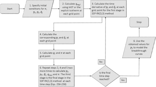
4.8. Pulse breakthrough

RUPTURA also includes pulse-style breakthrough curve modelling. Instead of using a step input for the adsorbing components of the mixture, a pulse input is used. The pulse breakthrough curve allows us to identify whether the adsorbent is able to fractionate different components in a mixture [232]. The breakthrough curves are dome shaped. The inlet concentrations for the adsorbing components become zero after the specified time period. On reaching the maximum concentration, the breakthrough curve gradually falls back to zero concentration level. If there is sufficient time gap between the peaks of the breakthrough curves for the components in a mixture, then it indicates that the adsorbent is suitable for the separation of the components.

All the equations and the conditions remain identical to the step breakthrough model, except for the inlet boundary conditions for the components in the mixture. The modified boundary conditions are shown below. (295) $p_i(t,z=0)=\{\begin{array}{cc}{p}_i^{\mathrm{i}\mathrm{n}},0\le & t<t_{\mathrm{p}\mathrm{u}\mathrm{l}\mathrm{s}\mathrm{e}}\\ 0,& t\ge t_{\mathrm{p}\mathrm{u}\mathrm{l}\mathrm{s}\mathrm{e}}\end{array}$(295) (296) $p_{\mathrm{c}\mathrm{a}\mathrm{r}\mathrm{r}\mathrm{i}\mathrm{e}\mathrm{r}\mathrm{g}\mathrm{a}\mathrm{s}}(t,z=0)=\{\begin{array}{cc}{p}_{\mathrm{c}\mathrm{a}\mathrm{r}\mathrm{r}\mathrm{i}\mathrm{e}\mathrm{r}\mathrm{g}\mathrm{a}\mathrm{s}}^{\mathrm{i}\mathrm{n}},0\le & t<t_{\mathrm{p}\mathrm{u}\mathrm{l}\mathrm{s}\mathrm{e}}\\ p_{{}_T}^{\mathrm{i}\mathrm{n}},& t\ge t_{\mathrm{p}\mathrm{u}\mathrm{l}\mathrm{s}\mathrm{e}}\end{array}$(296) In Equations (295(295) $p_i(t,z=0)=\{\begin{array}{cc}{p}_i^{\mathrm{i}\mathrm{n}},0\le & t<t_{\mathrm{p}\mathrm{u}\mathrm{l}\mathrm{s}\mathrm{e}}\\ 0,& t\ge t_{\mathrm{p}\mathrm{u}\mathrm{l}\mathrm{s}\mathrm{e}}\end{array}$(295) ) and (296(296) $p_{\mathrm{c}\mathrm{a}\mathrm{r}\mathrm{r}\mathrm{i}\mathrm{e}\mathrm{r}\mathrm{g}\mathrm{a}\mathrm{s}}(t,z=0)=\{\begin{array}{cc}{p}_{\mathrm{c}\mathrm{a}\mathrm{r}\mathrm{r}\mathrm{i}\mathrm{e}\mathrm{r}\mathrm{g}\mathrm{a}\mathrm{s}}^{\mathrm{i}\mathrm{n}},0\le & t<t_{\mathrm{p}\mathrm{u}\mathrm{l}\mathrm{s}\mathrm{e}}\\ p_{{}_T}^{\mathrm{i}\mathrm{n}},& t\ge t_{\mathrm{p}\mathrm{u}\mathrm{l}\mathrm{s}\mathrm{e}}\end{array}$(296) ), $t_{\mathrm{p}\mathrm{u}\mathrm{l}\mathrm{s}\mathrm{e}}$ is the time period for which the inlet concentrations of the adsorbing components are non-zero.

Figures 12(a,b) show examples of pulse-style breakthrough curves for the mixture of ${\mathrm{C}}_6$ isomers: n-hexane $\left({\mathrm{n}\mathrm{C}}_6\right)$, 3-methyl pentane $\left(3{\mathrm{m}\mathrm{C}}_5\right)$, 2,2-dimethyl butane $\left(22{\mathrm{d}\mathrm{m}\mathrm{C}}_5\right)$, and 2,3-dimethyl butane $\left(23{\mathrm{d}\mathrm{m}\mathrm{C}}_4\right)$ in BEA-type zeolite at 523K and 12 bar. The dome-shaped breakthrough curves of and $22{\mathrm{d}\mathrm{m}\mathrm{C}}_4$ are very close to each other which means the separation of these two isomers is difficult. It is easier to separate ${\mathrm{n}\mathrm{C}}_6$ and $\left(22{\mathrm{d}\mathrm{m}\mathrm{C}}_5\right)$ for the operating conditions mentioned in Figure 12. This is because the peaks of their breakthrough curves are separated by a considerable time gap. A longer column (Figure 12(b)) enhances separation. However, the trade-off is that the retention time inside the bed increases for the adsorbing components. As a result, the amount of a specific component recovered will be lower for the longer column. This can be clearly seen in Figure 12. The peaks of the breakthrough curves in Figure 12(b) are shorter than those in Figure 12(a).

4.9. Validation

Jolimaitre et al. [233] considered the separation of mono and di-branched hydrocarbons in MFI-type (silicalite) zeolite. This study includes both experimental analysis and a breakthrough curve model. To validate our model, we use the experimental breakthrough curve data generated by Jolimaitre et al. [233]. It involves the separation of 2-methyl butane $\left(2{\mathrm{m}\mathrm{C}}_4\right)$ and 2-methyl pentane $\left(2{\mathrm{m}\mathrm{C}}_5\right)$. The experiments are conducted at 473 K and 5 bar and Nitrogen $\left({\mathrm{N}}_2\right)$ is used as the carrier gas.

Figure 12. (Colour online) Examples of pulse-style breakthrough curve simulation for the mixture of ${\mathrm{C}}_6$ isomers: n-hexane $\left({\mathrm{n}\mathrm{C}}_6\right)$, 3-methyl pentane $\left(3{\mathrm{m}\mathrm{C}}_5\right)$, 2,2-dimethyl butane $\left(22{\mathrm{d}\mathrm{m}\mathrm{C}}_4\right)$, and 2,3-dimethyl butane $\left(23{\mathrm{d}\mathrm{m}\mathrm{C}}_4\right)$ in BEA-type zeolite at 523 K and 12 bar. Isothermal and isobaric conditions are imposed on the fixed bed column of length (a) 0.1 m and (b) 0.5 m. The bed porosity $\left({ϵ}_{{}_B}\right)$ is 0.2. Helium is used as the carrier gas. The inlet mole fractions for the ${\mathrm{C}}_6$ isomers are considered to be 0.01975. The interstitial velocity (v) at the inlet is 0.019 ms${}^{-1}$. 5s is the pulse time $\left(t_{\mathrm{p}\mathrm{u}\mathrm{l}\mathrm{s}\mathrm{e}}\right)$.

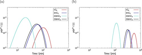
Experimental breakthrough conditions for the separation of $2{\mathrm{m}\mathrm{C}}_4$ and $2{\mathrm{m}\mathrm{C}}_5$ in MFI-type zeolite are shown in Table 9 [233]. This includes the inlet concentrations of the components in the mixture $\left(c_i^{\mathrm{i}\mathrm{n}}\right)$, their corresponding partial pressures $\left(p_i^{\mathrm{i}\mathrm{n}}\right)$ and mole fraction $\left(y_i^{\mathrm{i}\mathrm{n}}\right)$. The interstitial velocity (v) at the inlet is 0.0197 $\left[{\mathrm{m}\mathrm{s}}^{-1}\right]$ [233] and the bed porosity $\left({ϵ}_{{}_B}\right)$ is 0.4.

Table 9. Experimental conditions for separation of $2{\mathrm{m}\mathrm{C}}_4$, $2{\mathrm{m}\mathrm{C}}_5$.

	$c_i^{\mathrm{i}\mathrm{n}}/$ [mol m${}^{-3}$]	$p_i^{\mathrm{i}\mathrm{n}}/$ [bar]	$y_i^{\mathrm{i}\mathrm{n}}$
$2{\mathrm{m}\mathrm{C}}_4$	6.27	0.245	0.049
$2{\mathrm{m}\mathrm{C}}_5$	6.60	0.260	0.052

Notes: It includes the inlet concentrations $\left(c_i^{\mathrm{i}\mathrm{n}}\right)$, corresponding partial pressures $\left(p_i^{\mathrm{i}\mathrm{n}}\right)$ and the mole fractions $\left(y_i^{\mathrm{i}\mathrm{n}}\right)$.

Table 10. Values of dispersion coefficient $\left(\mathcal{D}\right)$ and mass transfer coefficient (k) for $2{\mathrm{m}\mathrm{C}}_4$ and $2{\mathrm{m}\mathrm{C}}_5$.

	$\mathcal{D}/$ [m${}^2$ s${}^{-1}$]	$k/$ [s${}^{-1}$]
$2{\mathrm{m}\mathrm{C}}_4$	$4.79\cdot {10}^{-5}$	0.056
$2{\mathrm{m}\mathrm{C}}_5$	$3.91\cdot {10}^{-5}$	0.051

Notes: The coefficients are calculated at 473 K and 5bar for the composition shown in Table 9.

The axial dispersion coefficients $\left(\mathcal{D}\right)$ are calculated using the following equation as shown in Table 7: (297) $\mathcal{D}=(0.45+0.55{ϵ}_{{}_B})D_m+0.5d_{{}_P}v$(297) In Equation (297(297) $\mathcal{D}=(0.45+0.55{ϵ}_{{}_B})D_m+0.5d_{{}_P}v$(297) ), $D_m$ is the molecular diffusion coefficient in $\left[{\mathrm{m}}^2{\mathrm{s}}^{-1}\right]$, $d_{{}_P}$ is the particle diameter in $\left[\mathrm{m}\right]$ and v is the velocity of the fluid phase in .

The mass transfer coefficient (k) is calculated using Equation (235(235) $\frac{\mathrm{d}\overline{q}}{\mathrm{d}t}=k(q_{{}_S}-\overline{q})$(235) ). This equation shows that k is proportional to the effective diffusion coefficient, $\left(D^{\mathrm{e}\mathrm{f}\mathrm{f}}\right)$ which is obtained as follows [6]: (298) $D^{\mathrm{e}\mathrm{f}\mathrm{f}}={(\frac{1}{D_m}+\frac{1}{D_{{}_K}})}^{-1}$(298) In Equation (298(298) $D^{\mathrm{e}\mathrm{f}\mathrm{f}}={(\frac{1}{D_m}+\frac{1}{D_{{}_K}})}^{-1}$(298) ), $D_m$ is the molecular diffusion coefficient and $D_{{}_K}$ is the Knudsen diffusion coefficient. The units of both the diffusivities are in $\left[{\mathrm{m}}^2{\mathrm{s}}^{-1}\right]$. $D_m$ is obtained using Equations (215(215) $D_m=\frac{A{T}^{\frac{3}{2}}}{p{\sigma }_{12}^2\mathrm{\Omega }}{(\frac{1}{M_1}+\frac{1}{M_2})}^{0.5}$(215) ). The expression for Knudsen diffusivity is shown below. (299) $D_{{}_K}=\frac{d_{\mathrm{p}\mathrm{o}\mathrm{r}\mathrm{e}}}{3}\sqrt{\frac{8RT}{\pi M}}$(299) In Equation (299(299) $D_{{}_K}=\frac{d_{\mathrm{p}\mathrm{o}\mathrm{r}\mathrm{e}}}{3}\sqrt{\frac{8RT}{\pi M}}$(299) ), $d_{\mathrm{p}\mathrm{o}\mathrm{r}\mathrm{e}}$ is the pore diameter, R is the universal gas constant, T is the temperature and M is the molar mass of the component. The values of dispersion coefficients $\left(\mathcal{D}\right)$ and mass transfer coefficients (k) for $2{\mathrm{m}\mathrm{C}}_4$ and $2{\mathrm{m}\mathrm{C}}_5$ at 473K and 5bar total pressure are shown in Table 10.

Pure component adsorption isotherms are modelled using single site Langmuir isotherms. The parameters $\left(q^{\mathrm{s}\mathrm{a}\mathrm{t}}\right)$ and (b) obtained from fitting the Langmuir isotherm to the adsorption loading data are shown in Table 11. The adsorption loadings for the pure components are obtained using grand-canonical Monte Carlo (GCMC) simulations [83] .

Table 11. Pure component adsorption isotherm parameters.

	$q^{\mathrm{s}\mathrm{a}\mathrm{t}}/$ [mol/(kg framework)]	$b/$ [Pa${}^{-1}$]
$2{\mathrm{m}\mathrm{C}}_4$	$0.717\pm 4\cdot {10}^{-3}$	$2.835\cdot {10}^{-5}\pm 7\cdot {10}^{-7}$
$2{\mathrm{m}\mathrm{C}}_5$	$0.699\pm 2\cdot {10}^{-3}$	$1.271\cdot {10}^{-4}\pm 3\cdot {10}^{-7}$

Notes: Single-site Langmuir isotherms are used to fit the pure component adsorption loading data obtained using GCMC simulations at 473 K. $q^{\mathrm{s}\mathrm{a}\mathrm{t}}$ is the saturation loading and b is the equilibrium constant.

Figure 13 shows the comparison between the breakthrough curves at the column exit for the mixture of $2{\mathrm{m}\mathrm{C}}_5$ and $2{\mathrm{m}\mathrm{C}}_4$ obtained from our simulation and the experiment performed by Jolimaitre et al. [233]. The breakthrough curves from the simulation and experiment follow similar trends. The discrepancies between the experimental and simulated fronts can occur because of several reasons such as errors in the pure component isotherm data, assumptions involved in IAST/SIAST model for equilibrium calculations, inaccurate estimation of the dispersion or/and diffusion coefficients, use of the LDF model, etc. Further, errors in conducting experiments and quality of the adsorbent and fluid phase sample can also cause these deviations.

Figure 13. (Colour online) Validation of the breakthrough curve model with the experimental results of Jolimaitre et al. [233]. This figure shows the separation of ${2\mathrm{m}\mathrm{C}}_4$ and ${2\mathrm{m}\mathrm{C}}_5$ in MFI-type zeolite at 473K and 5bar. The coloured squares represent the experimental data and the solid lines represent the results from our simulations.

The adsorption of $2{\mathrm{m}\mathrm{C}}_4$ is weaker compared to $2{\mathrm{m}\mathrm{C}}_5$. Therefore, $2{\mathrm{m}\mathrm{C}}_4$ is the first component to exit the column and shows a roll-up behaviour. The roll-up refers to the hump that occurs in the breakthrough curve of the weekly adsorbing component before the strongly adsorbing component starts to breakthrough. This behaviour occurs because the gas phase concentration of the strongly adsorbing component is continuously decreasing due to its adsorption. As a result, the partial pressure of the weakly adsorbing component increases and at certain time, it exceeds the inlet partial pressure (i.e. $p_i/p_i^{\mathrm{i}\mathrm{n}}>1$) [187]. The roll-up falls back to the inlet partial pressure, once the strongly adsorbing component starts to breakthrough and eventually reaches equilibrium.

4.10. Case study

In this section, we present a case study consisting of fitting of pure component loading data, mixture isotherm prediction, and breakthrough curve simulations. Here, we consider the case of adsorption of CO${}_2$ and C${}_3$H${}_8$ mixture in MOR-type zeolite at 300 K from Ref. [31]. Fitting of pure component loading data and estimation of mixture isotherms, and simulations of breakthrough curves were performed using RUPTURA. The pure component loading data were obtained using the RASPA software [21,22]. In this study, we also compare the influence of different mixture isotherm prediction models on the adsorption isotherms, and the breakthrough curves.

Figure 14(a) shows pure component isotherms (dual-site Langmuir) fitted to the adsorbed loadings obtained using Grand-Canonical Monte Carlo (GCMC) simulations. The unary isotherms show dual-site behaviour because MOR-type zeolite has two types of adsorption sites (pockets) [29,31]. Dual-site Langmuir isotherms have two pairs of fitted parameters (equilibrium constant and saturation loading) which are shown in Table 12. The MOR-type zeolite has a slightly higher loading of CO${}_2$ compared to C${}_3$H${}_8$. This indicates that the affinity of the structure with CO${}_2$ is higher than that of C${}_3$H${}_8$ and the preference for CO${}_2$ is energetic in nature in this regime. At higher pressure, entropy (packing) effects come into play. Here we see that also these effects are in favour of CO${}_2$ since CO${}_2$ shows a higher adsorption and higher saturation loading in the pure component isotherms.

Figure 14. (Colour online) Adsorption isotherms for CO${}_2$ and C${}_3$H${}_8$ in MOR-type zeolite at 300 K. (a) Unary isotherms (dual-site Langmuir) which are fitted to the pure component loading data obtained using RASPA, (b) comparison between mixture isotherms for equimolar composition of CO${}_2$ and C${}_3$H${}_8$ computed using IAST, SIAST and SEI.

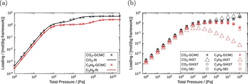
Table 12. Fitted parameters for the adsorption of pure ${\mathrm{C}\mathrm{O}}_2$ and ${\mathrm{C}}_3$ in MOR-type zeolite at 300 K.

	$b_1$	$q_1^{\mathrm{s}\mathrm{a}\mathrm{t}}$	$b_2$	$q_2^{\mathrm{s}\mathrm{a}\mathrm{t}}$
	$\left[1/\mathrm{P}\mathrm{a}\right]$	$\left[\mathrm{m}\mathrm{o}\mathrm{l}/\left(\mathrm{k}\mathrm{g}\mathrm{f}\mathrm{r}\mathrm{a}\mathrm{m}\mathrm{e}\mathrm{w}\mathrm{o}\mathrm{r}\mathrm{k}\right)\right]$	$\left[1/\mathrm{P}\mathrm{a}\right]$	$\left[\mathrm{m}\mathrm{o}\mathrm{l}/\left(\mathrm{k}\mathrm{g}\mathrm{f}\mathrm{r}\mathrm{a}\mathrm{m}\mathrm{e}\mathrm{w}\mathrm{o}\mathrm{r}\mathrm{k}\right)\right]$
${\mathrm{C}\mathrm{O}}_2$	$2.617\cdot {10}^{-4}$	1.60	$4.859\cdot {10}^{-7}$	3.62
	$\pm 3\cdot {10}^{-5}$	$\pm 5\cdot {10}^{-2}$	$\pm 3\cdot {10}^{-8}$	$\pm 5\cdot {10}^{-2}$
${\mathrm{C}}_3$	$6.506\cdot {10}^{-9}$	1.73	$2.376\cdot {10}^{-4}$	1.09
	$\pm 3\cdot {10}^{-10}$	$\pm 6\cdot {10}^{-3}$	$\pm 8\cdot {10}^{-6}$	$\pm 4\cdot {10}^{-3}$

Notes: Adsorbed loadings obtained from the GCMC simulations for the pressure range $({10}^0-5\cdot {10}^{10})$ Pa are fitted using the dual-site Langmuir isotherm.

Table 13. Fitted parameters for the adsorption isotherm (dual-site Langmuir-Freundlich) of o-xylene in MAF-x8-P1 zeolite at 433 K using different methods.

	$q_1^{\mathrm{s}\mathrm{a}\mathrm{t}}/$	$b_1/$	${\nu }_1/$	$q_2^{\mathrm{s}\mathrm{a}\mathrm{t}}/$	$b_2/$	${\nu }_2/$	RMSE/
	[mol/(kg framework)]	[Pa${}^{-1}$]	[–]	[mol/(kg framework)]	[Pa${}^{-1}$]	[–]	[mol/(kg framework)]
RUPTURA	1.9377	1.1132	0.2476	1.5793	$1.0485\times {10}^8$	1.2963	0.062
SciPy	1.9583	1.1334	0.2439	1.5617	$2.8218\times {10}^8$	1.3654	0.062
Gnuplot	1.9554	1.1305	0.2438	1.5642	$2.4394\times {10}^8$	1.3553	0.064
GAIAST	2.0059	1.1785	0.2337	1.5215	$3.2212\times {10}^9$	1.5360	0.066

Notes: In this table, unlike in Figure 20, the Gnuplot fit has been performed using initial values close to the final solution, to avoid being stuck in a local minimum.

We can examine what happens when CO${}_2$ and C${}_3$H${}_8$ compete with each other by doing explicit grand-canonical Monte Carlo mixture simulations. Indeed, as shown in Figure 14(b), at low loading, CO${}_2$ is adsorbed significantly more than C${}_3$H${}_8$. At high pressures, we note that competition can increase the loading of one species at the expense of another. Thus, in a mixture, the loading of a component can go down with pressure, something that can not happen in single-component isotherms (when the framework is kept rigid). In most scenarios, IAST does an excellent job predicting the mixture. However, the CO${}_2$ and C${}_3$H${}_8$ in MOR-type zeolite system is an exception caused by segregation effects. In Figure 14(b), we compare the mixture isotherms computed using IAST, SIAST, and SEI models for an equimolar mixture of CO${}_2$ and C${}_3$H${}_8$ inside MOR-type zeolite. For this system, IAST shows significant deviations from the GCMC data whereas SIAST and SEI are in excellent agreement with these data. IAST underpredicts the adsorbed loadings for C${}_3$H${}_8$ and overpredicts for CO${}_2$ adsorption. The reason for the failure in this system, is that IAST assumes a uniform adsorbent but MOR-type zeolite has two distinct types of adsorption sites with CO${}_2$ and C${}_3$H${}_8$ have very different affinities for the two types of sites [29]. Consequently, the competition due to adsorption will not be identical in both of these sites. IAST fails to capture this effect and leads to incorrect predictions of adsorbed loadings.

The segregation effect has a huge influence on the behaviour of the breakthrough curves. Figure 15 shows the breakthrough curves for CO${}_2$, and C${}_3$H${}_8$ inside MOR-type zeolite comparing the IAST, SIAST and SEI mixture predictions. The simulations parameters are: column length $\left(L\right)=0.3$ m, particle density $\left({\rho }_{{}_P}\right)=1711.06$ kg/m${}^3$, bed void fraction $\left({ϵ}_{{}_B}\right)=0.4$, inlet velocity $\left(v^{\mathrm{i}\mathrm{n}}\right)=0.1$ m/s, total pressure $\left(p_{{}_T}\right)=1$ bar, and the mass transfer coefficients (k) for CO${}_2$, and C${}_3$H${}_8$ in MOR-type zeolite are taken as 0.06 s${}^{-1}$. The difference in breakthrough behaviour between IAST and SIAST is striking. Note that the prediction is based on the same pure component isotherm models, but that the IAST and SIAST differ in the adsorption physics. This example serves as an example that mixture prediction should be validated by explicit grand-canonical Monte Carlo simulations to verify the correct choice of the mixture prediction model. Note that SIAST and SEI lead to almost identical breakthrough curves. SEI is the non-iterative version, and hence has advantages in terms of speed and stability.

Figure 15. (Colour online) Comparison between breakthrough curves obtained on implementing IAST, SIAST, and SEI to the breakthrough curve model. A mixture of CO${}_2$ and C${}_3$H${}_8$ in MOR-type zeolite at 300 K and 10${}^5$ Pa is considered. Each of these components constitutes 10% of the gas phase. Helium is used as the carrier gas. The adsorption column is operated in isothermal and isobaric conditions.

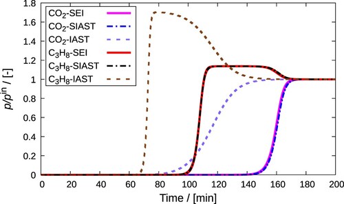
RUPTURA provides various options (IAST, SIAST, EI, and SEI) to estimate the mixture equilibrium loadings. One has to know apriori whether the adsorbent is heterogeneous and the adsorbing components prefer certain types of adsorption sites over the others. Knowledge of such information is essential in choosing the right mixture isotherm prediction model. If the adsorbent has distinct adsorption sites, then one should use SIAST [29], or SEI [31]. For uniform adsorbents, one can use IAST or EI. Also, it is important to note that for adsorbents with single type of adsorption sites, SIAST, and IAST are identical. Similarly, SEI, and EI are identical for uniform adsorbents. One should also be aware that EI and SEI can only be used if the pure component isotherms are Langmuir type.

Another important factor to consider is the effect of the number of grid points. A grid independence test is vital to determine the adequate number of grid points necessary for the breakthrough simulation. Here, we present a grid independence test for this case study. Three simulations are performed for this mixture with a different number of spatial grid points $(N_{\mathrm{g}\mathrm{r}\mathrm{i}\mathrm{d}}=20,50,\mathrm{a}\mathrm{n}\mathrm{d}100)$. In Figure 16, we can observe that the breakthrough curves generated using $N_{\mathrm{g}\mathrm{r}\mathrm{i}\mathrm{d}}=20$ are slightly different from those using $N_{\mathrm{g}\mathrm{r}\mathrm{i}\mathrm{d}}=50$. The differences in the breakthrough curves becomes smaller for $N_{\mathrm{g}\mathrm{r}\mathrm{i}\mathrm{d}}=50,\mathrm{a}\mathrm{n}\mathrm{d}100$. This indicates that the breakthrough curves undergo changes with increasing $N_{\mathrm{g}\mathrm{r}\mathrm{i}\mathrm{d}}$ to a certain limit. Beyond this point, these curves are invariant to an increase in the number of grid points.

Figure 16. (Colour online) Grid independence test on simulation of breakthrough curves for a mixture of CO${}_2$ and C${}_3$H${}_8$ in MOR-type zeolite at 300 K and 10${}^5$ Pa is performed. (a) Breakthrough curves simulated at different spatial grid points ($N_{\mathrm{g}\mathrm{r}\mathrm{i}\mathrm{d}}=20,50,\mathrm{a}\mathrm{n}\mathrm{d}100$), (b) certain zoomed in parts of the curves showing discrepancies due to the use of a different number of grid points. Each of these components constitutes 10% of the gas phase. Helium is used as the carrier gas. The adsorption column is operated in isothermal and isobaric conditions. With increasing the number of grid points, the breakthrough curves slightly changes. The variation becomes smaller between $N_{\mathrm{g}\mathrm{r}\mathrm{i}\mathrm{d}}=50\mathrm{a}\mathrm{n}\mathrm{d}100$.

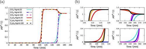
5. Isotherm fitting

5.1. Introduction

Curve fitting methods play an important role in many fields that involve system modelling and prediction techniques. Fitting is frequently used when it is necessary to match a complex model with (experimental) data [234,235]. The determination of a suitable set of parameters for an analytical model (the parametric function) can reveal insights into the underlying physical phenomena. The aim of this work is to accurately fit the pure component isotherm models (as described in Section 2) to isotherm data obtained from experiments or grand-canonical Monte Carlo simulations. The most common procedure in the literature is the use of analytical functions for model representation. It is also possible to interpolate data in a model-agnostic manner using e.g. cubic splines [236]. Simon et al. provided an interesting discussion on this topic [77]. Both simulation and experimental data have inherent noise, and when using numerical quadrature, there is always the danger of missing some physical information in an analytical model owing to over-fitting or over-interpreting the physical behaviour that is actually caused by errors in the data. Recently, Anderson and Gómez-Gualdróna [237] designed a method to predict the single-component adsorption of various small adsorbates (Xe, Kr, CH${}_4$, CH${}_6$, and N${}_2$) using machine learning techniques (‘multipurpose’ multilayer perceptron (MLP)). Using this method, these authors were able to predict thousands of mixing isotherms using a hybrid implementation of MLP-IAST. In RUPTURA, we developed our own implementation of a fitting tool for the isotherm models listed in Table 1.

5.2. Fitting methods

5.2.1. Linear fitting methods

A widely used technique to fit models to isotherm data is to carry out linear transformations on the isotherm data and then perform linear regression. Some isotherm models, such as Langmuir and Freundlich, can be estimated from linear regression, since these models can be linearised. Four linear transformations can be applied to the Langmuir isotherm ($\frac{q}{q^{\mathrm{s}\mathrm{a}\mathrm{t}}=\left(\frac{bp}{1+bp}\right)}$):

(1)	Double Reciprocal or Lineweaver-Burk transformation [238] ($\frac{1}{q}$ vs. $\frac{1}{p}$ plot, and $\frac{1}{q=\frac{1}{q^{\mathrm{s}\mathrm{a}\mathrm{t}}}+\frac{1}{q^{\mathrm{s}\mathrm{a}\mathrm{t}}bp}}$ transformation): It is strongly biased towards fitting the data in the low concentration range.
(2)	Reciprocal or Langmuir transformation [239] ($\frac{p}{q}$ vs. p plot, $\frac{p}{q=\frac{1}{b{q}^{\mathrm{s}\mathrm{a}\mathrm{t}}}+\frac{1}{bp}}$) tends to amplify the deviations from the fitted equation, highlighting outliers.
(3)	Eadie-Hofstee transformation [240,241] (q vs. $\frac{q}{p}$ plot, $\frac{q=q^{\mathrm{s}\mathrm{a}\mathrm{t}}-q}{bp}$ transformation). It has some bias toward fitting the data in the low concentration range.
(4)	Distribution Coefficient or Scatchard transformation [242] ($\frac{q}{p}$ vs. p plot, $\frac{q}{p=b{q}^{\mathrm{s}\mathrm{a}\mathrm{t}}-bq}$). It is biased toward fitting the data in the high concentration range.

Because the error distribution is modified and the weight of each point in the fit is transformation dependent, the result of the fit will depend on the choice of the linearisation method [243]. For this reason, the best fit is not the one with the highest correlation coefficient, but the one that predicts an error distribution that corresponds to to the original data. Single Langmuir behaviour is rare, and in most cases multiple-site isotherm models are needed. A more general approach is to use nonlinear regression [235].

5.2.2. Nonlinear least-squares (NLLS) fitting methods

In nonlinear regression problems, the aim is to find a parametric function (300) $y=f(x;\{a_k{\}}_{k=1}^M)$(300) which best fits a certain reference data set of points $(x_i,y_i{)}_{i=1}^N$ by minimising an error measure in the fitting. A widely used approach is to use the sum of squared residuals. The problem is thus mathematically defined as follows: (301) $\mathrm{W}\mathrm{S}\mathrm{S}\mathrm{E}=\sum _{i=1}^N{r}_i(x;\{a_k{\}}_{k=1}^M)=\sum _{i=1}^N{w}_i{(y_i-f(x_i;\left\{a_k{\}}_{k=1}^M\right))}^2$(301) (302) $\varphi ={\arg }_{\{a_k{\}}_{k=1}^M}\underset{x\in \chi }{min}\left(\mathrm{W}\mathrm{S}\mathrm{S}\mathrm{E}\right)$(302) where WSSE stands for Weighted Sum of the Squared Error (or cost function), ϕ is the value in the minimisation process, $r_i$ are the residual functions, and $w_i$ are the weights associated with each $(x_i,y_i)$–point. When the parametric function f is unknown, we have to choose a suitable model with a convenient set of M parameters $\left(a_k\right)$, and the error ϕ is minimised in an iterative way.

Gauss – Newton algorithm (GNA) [244]: In the Gauss-Newton method, the sum of squared errors is reduced by assuming that the least squares function is locally quadratic, and the minimum of the quadratic is obtained. The method is based on Newton's method to follow the curvature to the minimum, but does not use the Hessian of the residual function (which is computationally expensive), but the Jacobian of the residual functions, $r\left(\right\{a_k{\}}_{k=1}^M)$.

Steepest descent algorithm (SDA) [244]: In this method, also known as Gradient Descent, the sum of the squared errors is reduced by updating the parameters in the steepest-descent direction. This direction is calculated using the gradient, $-\mathrm{\nabla }r\left(\right\{a_k{\}}_{k=1}^M)$, and is therefore computationally cheap.

Marquardt–Levenberg algorithm (MLA) [245–249]: Developed by Levenberg, Girard, Wynne, Morrison, Marquardt. This method is actually a combination of two other NLLS fitting methods (GNA and SDA): It acts more like a SDA method when the parameters are far from their optimal value, and acts more like the GNA method when the parameters are close to their optimal values. This is the method used by the Gnuplot program, among others. An updated version of this method, which solves the problem of stacked solutions in local minimum, is the Trust Region Reflective method [250].

There are other widely used gradient-, Jacobian-, or Hessian-based algorithms to follow a path to find the minimum (whose computational efficiencies depend on the nature of the problem to be optimised): The Conjugate Gradient (CG) method [251], Broyden–Fletcher–Goldfarb–Shanno (BFGS) algorithm [252–255], and updates (e.g. Limited-memory BFGS [256]), the rational function optimisation algorithm (RFO), etc. In general, NLLS fitting is not guaranteed to converge to the global optimum from scratch (the solution with the smallest sum of squared residuals, SSR), and often gets stuck in a local minimum.

5.2.3. Heuristic fitting methods

Heuristic Search methods (Non-Math Optimisation algorithms) are not based on finding optimal analytic paths, based on gradients, Jacobians or Hessians, but explore the search space stochastically, keeping track of the ‘best’ points along the way. Two example approaches are discussed: the Nelder–Mead algorithm and genetic algorithm.

The Nelder–Mead algorithm (NMA) [117,257] is also called the downhill simplex method and was first introduced by Spendley et al. [257]. It is a heuristic search method based on the construction of a hypertetrahedron in M dimensions (a simplex) and how it adapts itself iteratively (by minimising the WSSE value) to the local landscape of the M-dimensional surface for the $\{a_k{\}}_{k=1}^M$ parameters. Each vertex ${\mathbf{a}}_{j=1}^{M+1}$ of this simplex is a vector with as many dimensions as there are parameters of the function f, i.e. ${\mathbf{a}}_j=(a_{1,j},a_{2,j},\dots ,a_{M,j})$. This is a local method and does not require derivatives.

The Genetic Algorithm (GA) [258,259] is a type of parallel heuristic search method. This method was described for the first time by De Jong [258] and Holland et al. [259]. The GA belongs to Evolutionary Algorithms (EA), a family of algorithms for global optimisation inspired by biological evolution, and uses biological operators inspired by biological evolution, such as reproduction, mutation, recombination, and selection. It is based on the generation of a population of individuals (each individual is a candidate for the optimisation solution) that are ordered according to their fitness. During the process, the population of solutions remains constant, and the worst solutions are replaced (by ranking its goodness–of–fit) by other solutions that are either mutation or recombination of better solutions. Some EA are as follows: Genetic Programming [260,261], Evolution Strategies [262], or Evolutionary Programming [263]. Other nature-inspired algorithms (but not part of the EA family) are: Particle Swarm Optimization (PSO) [264,265], Ant Colony Optimization (ACO) [266], Cuckoo Search (CS) [267], Grey Wolf Optimization (GWO) and updates [268,269], or Elephant Herd Optimization (EHO) [270,271].

GA is the most popular type of EA. In particular, GA represents each individual of the GA population as a string of numbers, usually a binary string called ”genotype”. Modifications in the genotype imply changes in the fitness. For some problems, it is convenient to use non-binary representations of the genotype.

5.3. Evaluating isotherm goodness–of–fit

In RUPTURA, we have used two standard measures for evaluating the goodness-of-fit: the Residual Root Mean Square Error (RMSE), and the correlation coefficient (r). We defined the RMSE as: (303) $\mathrm{R}\mathrm{M}\mathrm{S}\mathrm{E}={\left(\frac{\mathrm{W}\mathrm{S}\mathrm{S}\mathrm{E}}{N-M}\right)}^{\frac{1}{2}}$(303) where WSSE is the Weighted Sum of the Squared Error (Equation (301(301) $\mathrm{W}\mathrm{S}\mathrm{S}\mathrm{E}=\sum _{i=1}^N{r}_i(x;\{a_k{\}}_{k=1}^M)=\sum _{i=1}^N{w}_i{(y_i-f(x_i;\left\{a_k{\}}_{k=1}^M\right))}^2$(301) )), and N and M are the number of data points and the number of parameters of the model, respectively. The correlation coefficient r (usually $r^2$) is defined as: (304) $r=\frac{\sum _{i=1}^N(w_i{y}_i-\overline{y})\left(w_{i}f\right(x_i)-\overline{f})}{\sqrt{\sum _{i=1}^N(w_i{y}_i-\overline{y}{)}^2\sum _{i=1}^N\left(w_{i}f\right(x_i)-\overline{f}{)}^2}}$(304) For each optimisation iteration, RUPTURA monitors both values.

5.4. Software for isotherm fitting

Here we list some software proposed in the literature for isotherm fitting, as well as other general fitting software used for this purpose:

(1)	ISOTHERM and FIT programs [243,272,273]: This program is developed by Kinniburgh [272]. To the best of our knowledge, ISOTHERM appears in the literature as one of the first publicly available programs for isotherm fitting. Unfortunately, we have not been able to locate the code to test it.
(2)	ISOFIT [274]: ISOFIT was developed by Matott and Rabideau [274]. It is a program (executables available for Linux and Windows) that utilises a hybrid optimisation procedure combining Particle Swarm Optimization with Levenberg–Marquardt nonlinear regression. Many tools are available to check the quality of the fit. ISOFIT includes a wide collection of isotherm models (BET, Freundlich, Freundlich with Linear Partitioning, Langmuir-Freundlich, Langmuir, Langmuir with Linear Partitioning, Linear, Polanyi, Polanyi with Linear Partitioning, and Toth isotherms). However, it does not support fitting multisite isotherm models.
(3)	GAIAST [120]: GAIAST is developed by Balestra et al. [120]. Written in Fortran code (standard 2003), it has a module for isotherm fitting. The fitting module is coded using a constrained hybrid global optimisation procedure (NMA and GA). GA uses a single-precision floating-point format (binary32) to code the genotype. It presents a wide variety of isotherm models, from one to three adsorption sites, as well as some isobar models.
(4)	IAST++ [121]: IAST++ is developed by Lee et al. [121]. It is a Windows user-friendly executable program with a graphical user interface. It contains a module for suggesting isotherm models (among Langmuir, Langmuir-Freundlich, Langmuir Dual Site, Langmuir Freunclich Dual Site, BET, Quadratic, and Henry) based on the isotherm data entered, as well as visualisation of the fitting procedure. If the module does not find an acceptable isotherm model (based on goodness-of-fit) it suggests a quadratic interpolation. In practise, this module requires a fine-tuned selection of ranges in the generation of initial parameter values in order not to get stuck into local minima. This is particularly important for the Langmuir dual-site and Langmuir-Freundlich dual-site models.
(5)	Non-dedicated software: There is a large variety of open source tools, codes, and libraries for general purposes with which non-linear fits can be performed using different techniques. To mention a few of these: the SciPy Python Library [275] or the GNU Scientific Library (GSL) [276], or widely-used programs like Gnuplot [277], Octave [278]/ MATLAB [208], Origin [279] for NLLS methods, and the PIKAIA software [280] for GA methods.

5.5. Implementation of the GA-NMA hybrid method

In RUPTURA, we have implemented a constrained GA-NMA hybrid optimisation procedure that combines the GA (for an initial global search for the minimum), with the NMA method (to refine the founded best solutions). We employ the hybrid global optimisation method that was also used in the GAIAST code, but we have made significant improvements in speed and efficiency. RUPTURA uses hashing tables to map the genes, while GAIAST works with strings comparisons.

5.5.1. GA stage

We have used a concatenation of the 64-bit binary representation (double-precision floating-point format or just binary64) of the M parameters of the Equation (300(300) $y=f(x;\{a_k{\}}_{k=1}^M)$(300) ) to codified the genotype. There is a one-to-one relationship between the genotype and the sequence of parameters $\{a_j{\}}_{j=1}^M$ that is called the ”phenotype”. The parameter values of the isotherm models are constrained to a range of values to prevent nonphysical isotherm parameters (e.g. negative values for the saturation loading are not allowed). These constraints are hard-coded for each isotherm model.

The initial population is based on randomly generated isotherms from a range of initial values for each specified parameter. For example, the saturation values, $q^{\mathrm{s}\mathrm{a}\mathrm{t}}$, are generated between 0.0 to 10.0 [mol/(kg framework)], the b parameter between $1\times {10}^{-10}$ to $1\times {10}^{+10}$ [Pa${}^{-1}$], and the heterogeneity parameter, ν, anywhere between 0.1 to 2.1 [−]. If the isotherm parameters specified in the input files are non-zero, a refitting process is performed starting from these values.

In each optimisation step, k, we sort the population of individuals (called ”citizens”) according to its fitness and apply five biological operators on their genotype: elitism, crossover, mutation, replacement, and nuclear disaster. These GA operators are shown schematically in Figure 17.

Figure 17. (Colour online) Schematic representation of GA operators crossover, and mutation. The crossover operator is analogous to the crossover that happens during sexual reproduction in biology, and it combines the genotype of two parents to generate new offspring. We implemented three types of crossover operator: with one- and two points, and the uniform crossover. The mutation operator is activated before the children are added to the next generation.

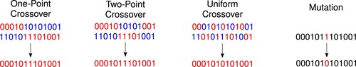
(1)	Elitism: We allow the best individuals ($\sim 5$%) of the current generation, k, to pass on unchanged to the next generation. In this way, we ensure that the best individual does not lose fitness in the optimisation process.
(2)	Replacement: The worst ($\sim 5$%) individuals are replaced by new individuals.
(3)	Crossover: We mate the population of the current generation (parents) to generate the next generation of individuals (children). We have implemented one-point, two-point, and uniform crossover, but using only the first one is sufficient to converge to a high-quality result. We perform a controlled mating between parents. Two types of crossover were carried out: between elitists (the group that ensures the goodness-of-fit) and between elitists and non-elitists (which provides the global character of the optimisation method).
(4)	Mutation: Some of the children, depending on the mutation rate value, do not pass unaltered to the next generation: We apply small changes in their genotype (see Figure 17).
(5)	Nuclear disaster: Only elitists are passed on to the next generation. The rest of the individuals are replaced by new individuals. This operator operates at a very low rate and is designed to escape from local minima. When this operator is activated, we break the cycle of operators and jump directly to the next generation, j + 1.

At the end of the operator cycle, we update the children to become parents and move on to the next generation, j + 1. During the optimisation process, RUPTURA prints the values of the genotype, phenotype (parameters), as well as the RMSE and the squared correlation coefficient, $r^2$, on the screen. As an example, for a step j = 114 of a Langmuir-Freundlich isotherm model fitting, it would look like:

mol: 0 step:  114 Fitness:  0.061057 R^2:  0.990488 Similarity:  2191/4096 Finishing:  80/100

number of parameters: 3

 genotype: 0011111111110011000000000000000000000000000000000000000000101100  parameter:  1.1875

 genotype: 0011111011111111111111111111111111111111111111111111111111111111  parameter:  3.05176e-05

 genotype: 0011111111110110000110110010000110011011001110111001110001010000  parameter:  1.38162

When the GA reached an optimal genotype ($r^2\to 1$ and $\mathrm{R}\mathrm{M}\mathrm{S}\mathrm{E}\to 0$ or RUPTURA has reached the maximum number of steps allowed), the candidate for the global minimum is refined during the NMA stage.

5.5.2. NMA (simplex) stage

We start with the parameter values corresponding to the phenotype of the best individual in the GA population. At each iteration k, the M + 1 vertices of the simplex, ${\mathrm{\Delta }}_k$, are converging to the minimum, and we sort and label the vertices according to Equation (302(302) $\varphi ={\arg }_{\{a_k{\}}_{k=1}^M}\underset{x\in \chi }{min}\left(\mathrm{W}\mathrm{S}\mathrm{S}\mathrm{E}\right)$(302) ), such that: (305) $\varphi \left({\mathbf{a}}_1\right)\le \varphi \left({\mathbf{a}}_2\right)\le \cdots \le \varphi \left({\mathbf{a}}_{M+1}\right),$(305) being ${\mathbf{a}}_1$ the best, and ${\mathbf{a}}_{M+1}$ the worst. In addition, we also calculate the centroid of the best M vertices, i.e.avoiding the worst: (306) $\overline{\mathbf{a}}=\sum _{i=1}^M\frac{{\mathbf{a}}_i}{M}$(306) Following the version of Lagarias et al. [281] of the Nelder–Mead algorithm, we updated the vertices by performing four possible operations: reflection, expansion, contraction, and shrinkage. Each of these operations are determined by a scalar: $\alpha =1$, $\text{β}=2$, $\frac{\gamma =1}{2}$, and $\frac{\delta =1}{2}$, respectively. We have used a version in which these scalars are constant, but there are modern implementations in which these parameters are adaptable [282]. In Figure 18 we show the algorithm of a single iteration step. In more detail, the four operations are

Figure 18. (Colour online) Flowchart of one step, k, in the Nelder-Mead algorithm [117] for a parametric function, f, with two parameters. In this way, the simplex is a triangle, and the visualisation is easier. The four operations and the sorting stage are in green labels.

(1)	Reflection: Once we have ordered the vertices according to Equation (305(305) $\varphi \left({\mathbf{a}}_1\right)\le \varphi \left({\mathbf{a}}_2\right)\le \cdots \le \varphi \left({\mathbf{a}}_{M+1}\right),$(305) ), and we have calculated the centroid of Equation (306(306) $\overline{\mathbf{a}}=\sum _{i=1}^M\frac{{\mathbf{a}}_i}{M}$(306) ), we proceed to calculate the reflected point, ${\mathbf{a}}_r$: (307) ${\mathbf{a}}_r=\overline{\mathbf{a}}+\alpha (\overline{\mathbf{a}}+{\mathbf{a}}_{M+1})$(307) We evaluate this point, $\varphi \left({\mathbf{a}}_r\right)$. If $\varphi \left({\mathbf{a}}_r\right)\le \varphi \left({\mathbf{a}}_r\right)<\varphi \left({\mathbf{a}}_M\right)$, then we accept the reflection point: ${\mathbf{a}}_{M+1}={\mathbf{a}}_r$.
(2)	Expansion: If $\varphi \left({\mathbf{a}}_r\right)\le \varphi \left({\mathbf{a}}_1\right)$ then we calculate the expansion point, ${\mathbf{a}}_e$: (308) ${\mathbf{a}}_e=\overline{\mathbf{a}}+\text{β}({\mathbf{a}}_r-\overline{\mathbf{a}})$(308) We evaluate this expansion point, $\varphi \left({\mathbf{a}}_e\right)$. If $\varphi \left({\mathbf{a}}_e\right)<\varphi \left({\mathbf{a}}_r\right)$ then we accept ${\mathbf{a}}_{M+1}={\mathbf{a}}_e$, otherwise we accept the reflection point: ${\mathbf{a}}_{M+1}={\mathbf{a}}_r$.
(3)	Contraction. (a) Outside: If $\varphi \left({\mathbf{a}}_M\right)\le \varphi \left({\mathbf{a}}_r\right)<\varphi \left({\mathbf{a}}_{M+1}\right)$ we perform an outside contraction: (309) ${\mathbf{a}}_{oc}=\overline{\mathbf{a}}+\gamma ({\mathbf{a}}_r-\overline{\mathbf{a}})$(309) and we evaluate the new point, $\varphi \left({\mathbf{a}}_{oc}\right)$. If $\varphi \left({\mathbf{a}}_{oc}\right)\le \varphi \left({\mathbf{a}}_r\right)$ then we accept the outside contraction point: ${\mathbf{a}}_{M+1}={\mathbf{a}}_{oc}$, else we perform a shrinkage operation. (b) Inside: If $\varphi \left({\mathbf{a}}_r\right)\ge \varphi \left({\mathbf{a}}_{M+1}\right)$ we perform an inside contraction: (310) ${\mathbf{a}}_{ic}=\overline{\mathbf{a}}-\gamma ({\mathbf{a}}_r-\overline{\mathbf{a}})$(310) and we evaluate the new point, $\varphi \left({\mathbf{a}}_{ic}\right)$. If $\varphi \left({\mathbf{a}}_{ic}\right)\le \varphi \left({\mathbf{a}}_{M+1}\right)$ then we accept the inside contraction point: ${\mathbf{a}}_{M+1}={\mathbf{a}}_{ic}$, else we perform a shrinkage operation.
(4)	Shrinkage: We generate the new vertices: (311) $<p>{\mathbf{v}}_i={\mathbf{a}}_1+\delta ({\mathbf{a}}_i-{\mathbf{a}}_1),\mathrm{\forall }i=2,\dots ,M+1.$(311) These will be the new vertices, ${\mathbf{a}}_{i=1}^{M+1}$, in the next iteration.

5.6. Validation

To validate the RUPTURA fitting function and compare it with other widely used codes (ISOFIT, IAST++, pyIAST, GAIAST, and Gnuplot; see Subsection 5.4) we fit the adsorption isotherms of n-C${}_7$ in BEA zeolite at 552 K. The isotherm exhibits a behaviour that can be modelled by many kinds of models: Langmuir, Langmuir-Freundlich, Sips, Toth, etc. We have chosen the Toth model of a single adsorption site (three parameters: $q^{\mathrm{s}\mathrm{a}\mathrm{t}},b,\mathrm{a}\mathrm{n}\mathrm{d}\nu$). For this relatively simple isotherm shape, all codes are able to accurately fit the isotherm model to the data, as shown in Figure 19. The obtained goodness-of-fits were $r^2>0.998$, and $\mathrm{R}\mathrm{M}\mathrm{S}\mathrm{E}<$ 0.025 [mol/(kg framework)], even form scratch. ISOFIT++ does not have incorporated the Toth model. The fitting of the isotherm using the Langmuir model using the IAST++ code gave reasonable results (RMSE = 0.025 [mol/(kg framework)]). RUPTURA takes 1.1 s to do this fit using a single core Intel Core i7-10700K CPU at 3.80 GHz.

Figure 19. (Colour online) (Left) Adsorption of n-C${}_7$ in BEA zeolite at 552 K and some fitted models using ISOFIT, Gnuplot, IAST++, and RUPTURA for a Toth model of a single adsorption site. (Right) Predicted loading vale vs. observed loading values. The goodness-of-fit in colours (same code colour of the Left panel) for each code. The RMSE values are in [mol/(kg framework)] units.

A much more challenging case is the adsorption isotherm of o-xylene in MAF-X8 at 300 K. The isotherm shows, see Figure 20, two steep slopes at $1\times {10}^{-6}$ and 10 Pa around an inflection (‘kink’). By adding a third site to the model, it fits well to a third bend of the isotherm. Adding a fourth site does not qualitatively improve the model. We have modelled the isotherm using the Langmuir-Freundlich model with two adsorption sites. The dual-site Langmuir-Freundlich model has six parameters ($q_1^{\mathrm{s}\mathrm{a}\mathrm{t}},b_1,{\nu }_1,q_2^{\mathrm{s}\mathrm{a}\mathrm{t}},b_2,\mathrm{a}\mathrm{n}\mathrm{d}{\nu }_2$). In general, for an increased number of model parameters, it is more likely that local minima will appear, and global optimisation algorithms become necessary.

Figure 20. (Colour online) (Left) Adsorption of o-xylene in MAF-X8 zeolite at 300 K and some fitted models using IAST++, Gnuplot (from scratch), GAIAST, and RUPTURA for a dual-site Langmuir-Freundlich model. (Right) Predicted loading vale vs. observed loading values. The goodness-of-fit for each code in colours defined in the left panel. The RMSE values are in [mol/(kg framework)] units.

GAIAST and RUPTURA predict equivalent values (the fitting algorithms are very similar), but RUPTURA is much more optimised and performs the same fitting in ten times less time, with goodness-of-fit values of $\mathrm{R}\mathrm{M}\mathrm{S}\mathrm{E}\le 0.066$ [mol/(kg framework)] and $r^2=0.998$. However, the optimisations from scratch using pyIAST (not shown in the Figure), Gnuplot (from scratch), or IAST++, with $\mathrm{R}\mathrm{M}\mathrm{S}\mathrm{E}\ge 0.312$ [mol/(kg framework)] were unable to accurately fit the model. That is, the error is too large for the model to represent the isotherm data well and to be used in IAST or breakthrough calculations). Only if the starting values are chosen close to the solution is Gnuplot able to generate models with high goodness of fit (see Table 13). RUPTURA takes 2.6 s to do this fit, and GAIAST, 26 s. If we consider a Langmuir-Freundlich with three sites (nine parameters) for the model in the fitting procedure, RUPTURA takes 6.279 s, obtaining $\mathrm{R}\mathrm{M}\mathrm{S}\mathrm{E}=0.0385$ [mol/(kg framework)], and $r^2=0.9993$. However, erroneous results could be obtained by overfitting a simple isotherm with an unnecessary complex model. Regardless of this issue, RUPTURA is able to quickly optimise difficult isotherms (with multiple minima) as shown in Figure 21.

Figure 21. (Colour online) The adsorption isotherm prediction for two, three, and four sites Langmuir-Freundlich isotherm models for o-xylene in MAF-X8. Without the experimental error information for the loading data is difficult to establish what kind of model is more realistic.

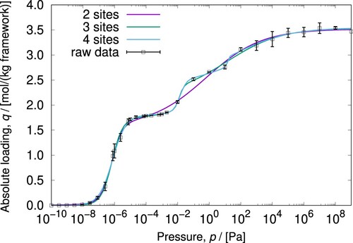
A particularly difficult test case is alkane C6 isomers in MAF-6 at 298 K with a relatively small amount of points, but with small error bars. Figure 22 shows that RUPTURA produces excellent fits using dual- and triple-site Langmuir-Freundlich models. The shape of the isotherms, combined with smooth and sharply rising slopes over many orders of magnitude of pressure, poses a challenge for the fit. Note that using a small amount of points over a large pressure range (equally distributed in log-scale) is a very common scenario to explore the overall shape of the isotherms.

Figure 22. (Colour online) The C${}_6$-alkane-isomers adsorption isotherms in MAF-6 computed from grand-canonical Monte Carlo simulations fitted with dual- and triple site Langmuir-Freundlich isotherm models. The peculiar shape of these isotherms in the low-pressure region makes this system challenging to preform reliable fitting.

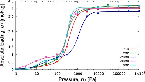
Lastly, we used Python SciPy Library to test the RUPTURA code (see Listing 1). Scipy (scipy.optimize.curve_fit) uses the Trust Region Reflective (TRR) method for constrained problems [283,284]. The TRR method is an evolution of the Levenberg-Marquardt algorithm, but with global convergence. In Figures 19 and 20, as well as Table 13, you can see that RUPTURA gives goodness-of-fit comparable to TRR.

Listing 1. Python script used to fit isotherms with Toth and dual-site Langmuir-Freundlich models using the SciPy Library.]

import pandas as pd

import numpy as np

import matplotlib.pyplot as plt

from scipy.optimize import curve_fit

def Toth(P, q, b, n):

 return q * b * P / pow(1 + pow(b*P,n),(1.0/n))

def DSLangmuirFreundlich(P, q1, b1, n1, q2, b2, n2):

 return q1 * b1 * pow(P,n1) / (1 + b1 * pow(P,n1)) +

q2 * b2 * pow(P,n2) / (1 + b2 * pow(P,n2))

df = pd.read_csv('Results.dat-MAF-x8-P1-Repeat-433K-o-xylene', sep=' ')

popt, pcov = curve_fit(DSLangmuirFreundlich,

           df['P'].values, df['L'].values,

           p0=(1.0,1.0,1.0,1.0,1.0,1.0),

           bounds=([0,1.0E-20,0.1,0,1.0E-20,0.1],

           [100,1.0E+20,10.0,100,1.0E+20,10.0]))

print(*popt)

6. RUPTURA installation

For the basic functionality, only a c++11 compiler is needed. However, automatic picture generation is based on gnuplot [277], and automatic movie generation is based on gnuplot and ffmpeg [285]. FFmpeg needs to have support for HEVC/H.265 and/or H.264 video encoding.

The default colour scheme of gnuplot has several issues: the sequence of colours is hard to see for colour-blind people and yellow is hardly visible against a white background. We therefore use the colour scheme published in the book ‘Gnuplot in action’, stylesheet listing 12.7 [286]. All the required software tools are available as open source software.

6.1. Mac

Some additional software tools need to be installed. First, the Xcode Command Line Tools need to be installed. The easiest way to install Xcode Command Line Tools is by installing Homebrew, the popular package manager for macOS. When you install Homebrew, you will be offered the option of installing Xcode Command Line Tools. Go to the website https://brew.sh and copy and paste the installation command into a terminal. The command line tools include git, a version control system. Using homebrew, we can also install gnuplot and ffmpeg.

brew  install  gnuplot

brew  install  ffmpeg

Next, download RUPTURA using git and compile the code

git clone https://github.com/iraspa/ruptura

cd ruptura

cd src

make

6.2. Linux

Some additional software tools need to be installed. For Ubuntu-based systems

sudo apt install git build-essential gnuplot ffmpeg

Next, download RUPTURA using git and compile the code

git clone https://github.com/iraspa/ruptura

cd ruptura

cd src

make

6.3. Windows

Some additional software tools need to be installed.

• git

  The most official build is available for download on the Git website. Just go to https://git-scm.com/download/win and the download will start automatically.

• gnuplot

  Go to https://sourceforge.net/projects/gnuplot/files/gnuplot/ to download gnuplot, and install it via the binary installer. Preferably install gnuplot in C:\Program Files\gnuplot, or alternatively add the directory C:\Program Files\gnuplot\bin to the PATH variable.

• ffmpeg

  Go to https://github.com/BtbN/FFmpeg-Builds/releases, and download ffmpeg-master-latest-win64-gpl.zip. Unzip, and preferably install ffmpeg in C:\Program Files\ffmpeg-master-latest-win64-gpl, or alternatively add the directory C:\Program Files\ffmpeg-master-latest-win64-gpl\bin to the PATH environment variable.

Next, download RUPTURA using git

git clone https://github.com/iraspa/ruptura

A binary executable src/ruptura.exe for windows is already provided.

7. RUPTURA input description

7.1. General

All input is case-insensitive and white space does not matter. Font keyword means the literal text, [a$|$b] means the input of either a or b, [real] means the expected number is a floating point value, [int] means an integer is expected, and [string] means a string is expected. Strings are not allowed to contain spaces (replaces these by dashes or underscores). Numbering of indices starts at zero.

7.2. Simulation types

• SimulationType [MixturePrediction $|$ Breakthrough $|$ Fitting]

  Selects the type of the simulation. MixturePrediction selects the computation of a mixture based on pure component isotherms, the pressure-range, and the fluid-phase mole fractions. Breakthrough selects the computation of a mixture adsorbing in a fixed-bed adsorber. Fitting selects the computation of the best fit of an analytic isotherm model to raw adsorption data.

7.3. Component information

• Component [int] MoleculeName [string]

  The index of the component and the name of the component. The component name is used in the automatically generated plot-files and movies.

• Filename [string]

  The name of a file associated with this component. Used in fitting to specify the raw data of the isotherm.

• CarrierGas [yes$|$no]

  Specifies whether this component is the carrier-gas in a breakthrough simulation. There can be only one carrier-gas and a breakthrough simulation must contain a carrier gas. For the carrier gas there is no need to specify an isotherm model (the carrier gas is assumed to not adsorb).

• GasPhaseMolFraction [real]

  The dimensionless gas-phase mole fraction of the component. The values of all the components should sum up to unity, but if not, the code gives a warning and continues with the explicitly normalised mole fractions.

• MassTransferCoefficient [real]

  The mass-transfer coefficient of this component used in the Linear Driving Force (LDF) model. Units: 1/s.

• AxialDispersionCoefficient [real]

  The coefficient of axial mixing attribute to a diffusion-like process. Units: m${}^2$/s.

• NumberOfIsothermSites [int]

  The number of isotherm sites associated with this component. This keyword is followed by a list of isotherm models and parameters chosen from (See Table 1 for definition of the models):

  • Langmuir [real] [real]

    $b_0$ in mol kg${}^{-1}$, $b_1$ in Pa${}^{-1}$.

  • Anti-Langmuir [real] [real]

    $b_0$ in mol kg${}^{-1}$ Pa${}^{-1}$, parameter $b_1$ in Pa${}^{-1}$.

  • BET [real] [real] [real]

    $b_0$ in mol kg${}^{-1}$, $b_1$ dimensionless, $b_2$ dimensionless.

  • Henry [real]

    $b_0$ in mol kg${}^{-1}$ Pa${}^{-1}$.

  • Freundlich [real] [real]

    $b_0$ in mol kg${}^{-1}$ Pa${}^{-1}$, $b_1$ dimensionless.

  • Sips [real] [real] [real]

    $b_0$ in mol kg${}^{-1}$, $b_1$ in Pa${}^{-1}$.

  • Langmuir-Freundlich [real] [real] [real]

    $b_0$ in mol kg${}^{-1}$, $b_1$ in Pa${}^{-1}$, $b_2$ dimensionless.

  • Redlich-Peterson [real] [real] [real]

    Parameter $b_0$ in mol kg${}^{-1}$ Pa${}^{-1}$, parameter $b_1$ in Pa${}^{-1}$, $b_2$ dimensionless.

  • Toth [real] [real] [real]

    Parameter $b_0$ in mol kg${}^{-1}$, parameter $b_1$ in Pa${}^{-1}$, $b_2$ dimensionless.

  • Unilan [real] [real] [real]

    Parameter $b_0$ in mol kg${}^{-1}$, parameter $b_1$ in Pa${}^{-1}$, parameter $b_2$ dimensionless.

  • O'Brien&Myers [real] [real] [real]

    Parameter $b_0$ in mol kg${}^{-1}$, parameter $b_1$ in Pa${}^{-1}$, parameter $b_2$ dimensionless.

  • Quadratic [real] [real] [real]

    Parameter $b_0$ in mol kg${}^{-1}$, parameter $b_1$ in Pa${}^{-1}$, parameter $b_2$ in Pa${}^{-2}$.

  • Temkin [real] [real] [real]

    Parameter $b_0$ in mol kg${}^{-1}$, parameter $b_1$ in Pa${}^{-1}$, parameter $b_2$ dimensionless.

  • Bingel&Walton [real] [real] [real]

    Parameter $b_0$ in mol kg${}^{-1}$, parameter $b_1$ in Pa${}^{-1}$, parameter $b_2$ in Pa${}^{-1}$.

7.4. Mixture prediction

The mixture prediction module predicts, using various possible theoretical models, the adsorbed phase mole fractions based on pure component isotherms only.

• MixturePredictionMethod [IAST $|$ SIAST $|$ EI $|$SEI]

  The method used to predict the mixture adsorption based on pure component isotherm information. IAST denotes the Ideal Adsorption Solution Theory (IAST) [28], and SIAST is segregated IAST where IAST is applied to sites individually [29]. EI is the explicit isotherm model (not iterative and hence very fast) that is applicable to Langmuir models only [30,31]. SEI is the segregated explicit isotherm model. These models are explained in Sections 3.4 and 3.5 Default: IAST.

• IASTMethod [FastIAS $|$ Bisection]

  The method used to compute the IAST mixture prediction. Default: FastIAS.

• PressureStart [real]

  The lowest pressure of the range of pressures to be evaluated. Must be smaller than PressureEnd. Units: Pa.

• PressureEnd [real]

  The highest pressure of the range of pressures to be evaluated. Must be larger than PressureStart. Units: Pa.

• NumberOfPressurePoints [int]

  The number of points equally spaced in log-scale or linear scale.

• PressureScale [log$|$linear]

  The scale of the range of pressures, either logarithmic scale (log) or linear (linear).

7.5. Breakthrough

The breakthrough module allows the computation and evaluation of the performance of a fixed bed adsorber. A fixed bed packed with particles containing a porous material is pressurised and purged with a carrier gas. A (mixture-) fluid is added to the carrier gas, resulting in a step-wise change of the inlet concentration. In chromatographic separation processes, a pulse-wise change of the inlet concentrations is used. The change of the component concentrations along the column and at the outlet of the fixed bed are recorded.

7.6. Simulation duration

• BreakthroughType [step$|$ pulse]

  Selects a step breakthrough initial condition at the inlet, or a pulse condition as explained in Sections 4.7 and 4.8

• Pulselength [real]

  The length in time of the pulse condition at the inlet. Units: s, default: 10.0.

• NumberOfTimeSteps [int$|$ auto]

  Explicitly set the the number of time steps of the breakthrough computation or (only for step-breakthrough) let the program determine when the breakthrough computation is converged (auto).

• TimeStep [real]

  The time step used in the numerical integration scheme. Units: s, default: 0.0005.

• PrintEvery [int]

  How frequently to write status information to the screen. Default: 10,000.

• WriteEvery [int]

  How frequently to write data to the output files. Default: 10,000.

7.7. Column properties

• DisplayName [string]

  The name of the column, or material, that will be displayed in the output files (plots and movies).

• ColumnVoidFraction [real]

  The typical value of the fixed-bed porosity or bulk void fraction is ${ϵ}_{{}_B}$=0.38-0.40. Units: -, default: 0.4.

• ParticleDensity [real]

  The particle density ${\rho }_{{}_P}$ (density of the adsorbent grain) includes the inner porosity, but excludes the void fraction of the bed. Units: kg/m${}^3$, default 1000.0.

• TotalPressure [real]

  The total pressure at which to compute the breakthrough. Units: Pa, default: $1e6$.

• PressureGradient [real]

  The gradient of the pressure along the column. Units: Pa/m, default: 0.

• ColumnEntranceVelocity [real]

  The interstitial velocity of the fluid at the entrance of the column. Units: m/s, default: 0.1.

• ColumnLength [real]

  The length of the column. Units: m, default: 0.3.

7.8. Integration settings

• NumberOfGridPoints [int]

  The number of grid points used in the spatial discretisation of the column. Default: 100.

7.9. Fitting

The fitting module allows the fitting of isotherm models on raw, computed or measured adsorption isotherms.

• ColumnPressure [int]

  The index of the column in the raw-data file containing the information on the pressure.

• ColumnLoading [int]

  The index of the column in the raw-data file containing the information on the absolute adsorption amount.

8. RUPTURA tutorial

8.1. Introduction

The tutorial examples are designed to be fast. The binary mixture breakthrough example of CO${}_2$/N${}_2$ in silicalite runs in a matter of seconds. This allows interactive computations for teaching purposes, where students can easily play around with the column properties and investigate how the separation would be influenced by the gas-phase mole fractions, the bed-void fraction, the length of the column, axial dispersion and mass-transfer coefficients, etc. The second example of C${}_6$-isomers in BEA-type zeolite is more advanced, but still runs in one or two minutes. Both examples make use of the explicit isotherm model developed by Van Assche et al. [30] (Section 3.4.6) for the prediction of the mixture isotherms.

8.2. Breakthrough of CO${}_2$/N${}_2$ in silicalite

The directory tutorial/Silicalite-CO2-N2/breakthrough contains the input file simulation.input:

SimulationType      Breakthrough

// Column settings

DisplayName       Silicalite

Temperature       313.0   // [K]

ColumnVoidFraction   0.4    // [-]

ParticleDensity     1144.03  // [kg/m^3]

TotalPressure      2.5e6   // [Pa]

PressureGradient    0.0    // [Pa/m]

ColumnEntranceVelocity 0.1    // [m/s]

ColumnLength       0.3    // [m]

// Run settings

NumberOfTimeSteps   auto

PrintEvery       1000

WriteEvery       200

TimeStep        0.01    // [s]

NumberOfGridPoints  30

MixturePredictionMethod ExplicitIsotherm

Component 0 MoleculeName          Helium

     GasPhaseMolFraction      0.9       // [-]

     CarrierGas           yes

Component 1 MoleculeName          CO2

     GasPhaseMolFraction      0.05      // [-]

     MassTransferCoefficient    0.06      // [1/s]

     AxialDispersionCoefficient 0.0       // [m^2/s]

     NumberOfIsothermSites     1

     Langmuir            2.858 1.089e-5 // [mol/(kg framework)] [1/Pa]

Component 2 MoleculeName         N2

     GasPhaseMolFraction     0.05      // [-]

     MassTransferCoefficient   0.06      //   [1/s]

     AxialDispersionCoefficient 0.0       //   [m^2/s]

     NumberOfIsothermSites    1

     Langmuir          2.094 0.111e-5 // [mol/(kg framework)] [1/Pa]

The simulation-type is set to breakthrough, the column properties and run settings are specified, and lastly the information on all the components. The component information starts with the keyword Component followed by the component index (starting from zero) and the name of the component. The properties set after this line refer to the component denoted by the Component keyword. A component requires isotherm information except for the carrier gas. There must be a component labeled as carrier-gas and there can be only one. The isotherm information for the carrier has is implicitly a Langmuir isotherm with affinity parameter set to zero. For a component that is not the carrier gas, the number of isotherm sites need to be specified, followed by a list of isotherm models along with its parameters. A component also needs a gas-phase mol-fraction and mass-transfer coefficient, while the axial dispersion coefficient is optional.

The code is executed on mac/linux by typing in the terminal

./run

On windows you can run it from the windows console using the run.bat batch script, or by double-clicking on it. After a few seconds, the program is finished and many new files have been created

column.data            make_movie_Pnorm   plot_column_P

component_0_Helium.data make_movie_Pt     plot_column_Pnorm

component_1_CO2.data   make_movie_Q      plot_column_Pt

component_2_N2.data   make_movie_Qeq    plot_column_Q

make_graphs           make_movie_V     plot_column_Qeq

make_movie_Dpdt       make_movies      plot_column_V

make_movie_Dqdt       plot_column_Dpdt   plot_breakthrough

make_movie_P           plot_column_Dqdt

The column.data and component files are the files with the actual simulation data. make_movies creates movies to visualise the variation of different quantities along the length of the column. Dpdt and Dqdt represent time derivatives of the partial pressures and the adsorbed loadings of each component respectively. Movies are also created for the variation of the partial pressures (P), normalised pressure (ratio of partial pressure at the column exit to that at the inlet: Pnorm), total pressure (Pt), adsorbed loadings (Q), equilibrium loading (Qeq), and interstitial velocity (V) along the length of the fixed bed column. The plot_column files are used by the movie scripts to create figures for these measured quantities (using gnuplot). On windows, the make_movies and make_graphs scripts have the bat extension. By running these two scripts, the figures (breakthrough.pdf and breakthrough_dimensionless.pdf) and movies (files with .mp4 extension and file names starting with column_movie) will be created:

breakthrough.pdf          column_movie_Pnorm.mp4

breakthrough_dimensionless.pdf  column_movie_Pt.mp4

column_movie_Dpdt.mp4       column_movie_Q.mp4

column_movie_Dqdt.mp4       column_movie_Qeq.mp4

column_movie_P.mp4         column_movie_V.mp4

You could also run the individual make-movie scripts if you are interested only in some of them. The figures are in pdf files, the movies are in h265 format for mac/linux and h264 on windows, with resolution 1200x800 by default. On mac/linux, command line options can be specified to modify the defaults

./make_movies -e 5 -w 1600 -h 1200 -q 18 -l

The -e option stands for ‘every’ and allows a periodic sampling only using every 5 data -points in the example case. The -w and -h changes the width and height of the movie, while -q determines the quality of the movies. The quality range is 0–51, where 0 is lossless and 51 is worst quality possible. The default in RUPTURA is 18 which is visually nearly lossless. The -l option stands for legacy and changes the movie-format h265 to the older h264. On windows, these options can be specified in the windows console as

make_movies 5 1600 1200 18

Note the fixed order of the options, and the format on windows is h264 as h265 is not supported out-of-the-box under windows.

The output figures are shown in Figure 23(a). The breakthrough graph plots the normalised concentration at the exit of the column as a function of time. Two versions of the plots are available: (1) as a function of time in seconds, (2) as a function of dimensionless time. Figure 23(b) shows a single frame of the movie, here the loading of the components adsorbed in the crystallites along the column.

Figure 23. (Colour online) Breakthrough predictions of an equimolar mixture of CO${}_2$-N${}_2$ in silicalite at 313 K and $2.5\cdot {10}^6$ Pa: (a) breakthrough curve plot (file breakthrough_dimensionless.pdf) (b) movie frame of the loading inside the column (file column_movie_Q.mp4).

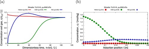
8.3. Mixture prediction of C${}_6$-isomers in BEA-type zeolite

For the C${}_6$-isomers in BEA-type zeolite example, we can test how well the explicit Langmuir models mixture adsorption in comparison with IAST. The directory tutorial/BEA-C6/mixture_prediction contains the input file simulation.input:

SimulationType       MixturePrediction

ColumnName         BEA

Temperature        552.0        // [K]

PressureStart       1e3         // lowest pressure

PressureEnd        1e7         // highest pressure

NumberOfPressurePoints  100         // number of points equally spaced

PressureScale       log         // [log, or linear]

MixturePredictionMethod  ExplicitLangmuir  // [IAST, SIAST, or ExplicitLangmuir]

Component 0 MoleculeName         Helium

     GasPhaseMolFraction     0.96       // [-]

     CarrierGas          yes

Component 1 MoleculeName         nC6

     GasPhaseMolFraction     0.01       // [-]

     NumberOfIsothermSites    1

     Langmuir           1.393 3.307e-05  // [mol/(kg framework)] [1/Pa]

Component 2 MoleculeName         C5m3

     GasPhaseMolFraction     0.01       // [-]

     NumberOfIsothermSites    1

     Langmuir            1.559 1.809e-05  // [mol/(kg framework)] [1/Pa]

Component 3 MoleculeName         C4m2m2

     GasPhaseMolFraction     0.01       // [-]

     NumberOfIsothermSites   1

     Langmuir           1.714 5.451e-06  // [mol/(kg framework)] [1/Pa]

Component 4 MoleculeName         C4m2m3

     GasPhaseMolFraction     0.01       // [-]

     NumberOfIsothermSites    1

     Langmuir            1.678 1.522e-05  // [mol/(kg framework)] [1/Pa]

Note the input is very similar in structure. The major difference is that the simulation-type is set to MixturePrediction. Using the option MixturePredictionMethod we can control the specific method used in the mixture prediction. Minor difference are that the mass-transfer and axial dispersion coefficients are not needed. To compute the mixture isotherm some info on the pressure range, i.e. begin and end-pressure and the number of pressure points is required. These points can be spread equi-distant in normal or in log-scale.

After running, the output directory contains the following plot-files.

component_0_Helium.data  component_4_C4m2m3.data  plot_mixture_mol_fractions

component_1_nC6.data    plot_mixture        plot_pure_components

component_2_C5m3.data    component_3_C4m2m2.data  make_graphs

Files with .data extension and file names starting with component consists of equilibrium loading data for the specified temperature, and the range of pressure. In windows, the script make_graphs has the bat extension. After running that script we obtain the plots in pdf format

mixture_prediction.pdf

mixture_prediction_mol_fractions.pdf

pure_component_isotherms.pdf

mixture_prediction.pdf file consists of the plots of mixture adsorption isotherms for all the components present in the mixture in the same unit specified for saturation loadings (q_sat) in the input file. mixture_prediction_mol_fractions.pdf file consists of the same plots in the form of mole fractions. pure_component_isotherms.pdf shows the plots for the isotherms for the pure components. In Figure 24, we can compare the pure components isotherms with the mixture isotherm predictions. In the mixture, we can see the effect of competitive adsorption.

Figure 24. (Colour online) Mixture predictions of a ${\mathrm{C}}_6$ isomer mixture in BEA- type zeolite at 552K using explicit isotherm model developed by Van Assche et al [30]: (a) pure components (file $\mathtt{p}\mathtt{u}\mathtt{r}\mathtt{e}\mathtt{\_}\mathtt{c}\mathtt{o}\mathtt{m}\mathtt{p}\mathtt{o}\mathtt{n}\mathtt{e}\mathtt{n}\mathtt{t}\mathtt{\_}\mathtt{i}\mathtt{s}\mathtt{o}\mathtt{t}\mathtt{h}\mathtt{e}\mathtt{r}\mathtt{m}\mathtt{s}\mathtt{.}\mathtt{p}\mathtt{d}\mathtt{f}$), (b) mixture prediction (file $\mathtt{m}\mathtt{i}\mathtt{x}\mathtt{t}\mathtt{u}\mathtt{r}\mathtt{e}\mathtt{\_}\mathtt{p}\mathtt{r}\mathtt{e}\mathtt{d}\mathtt{i}\mathtt{c}\mathtt{t}\mathtt{i}\mathtt{o}\mathtt{n}\mathtt{.}\mathtt{p}\mathtt{d}\mathtt{f}$).

8.4. Isotherm fitting

To obtain the isotherm model parameters we can use the fitting module. The directory tutorial/MAF-X8-xylenes contains the input file simulation.input:

SimulationType      Fitting

DisplayName        MAF-X8

ColumnPressure      3

ColumnLoading       8

PressureScale       log

Component 0 MoleculeName        p-xylene

     FileName           Results.dat-MAF-x8-P1-Repeat-433K-p-xylene

     NumberOfIsothermSites   2

     Langmuir-Freundlich    0.0 0.0 0.0

     Langmuir-Freundlich    0.0 0.0 0.0

 The result of the fit is printed at the end of the output.

  number of isotherm sites:  2

  Langmuir-Freundlich isotherm

    q_sat:  1.71616       // [mol/(kg framework)]

    b:   3.54859e+09     // [1/Pa]

    nu:   1.47094       // [-]

  Langmuir-Freundlich isotherm

    q_sat:  1.63797       // [mol/(kg framework)]

    b:   12.3201       // [1/Pa]

    nu:   0.515807      // [-]

File names starting with Results.dat consists of the equilibrium loading data computed using grand-canonical Monte Carlo simulations.

Results.dat-MAF-x8-P1-Repeat-433K-benzene

Results.dat-MAF-x8-P1-Repeat-433K-ethylbenzene

Results.dat-MAF-x8-P1-Repeat-433K-m-xylene

Results.dat-MAF-x8-P1-Repeat-433K-o-xylene

Results.dat-MAF-x8-P1-Repeat-433K-p-xylene

Results.dat-MAF-x8-P1-Repeat-433K-toluene

make_graphs

plot_fit_component_0_p-xylene

Again, using the make_graphs script, we can create the pdfs of the figures, e.g.

isotherms_fit_p-xylene.pdf

The result is plotted in Figure 25. It shows the initial random starting isotherm, and the final fit result after GA optimisation for adsorption of p-xylene in MAF-X8- type zeolite at 433 K.

Figure 25. (Colour online) Fitting a dual site Langmuir isotherm model to the pure component isotherm data for the adsorption of p-xylene in MAF-X8- type zeolite at 433 K. The pure component adsorbed loadings are computed using grand-canonical Monte Carlo simulations. The fitting is performed using genetic algorithm optimisation which is shown in the file $\mathtt{i}\mathtt{s}\mathtt{o}\mathtt{t}\mathtt{h}\mathtt{e}\mathtt{r}\mathtt{m}\mathtt{s}\mathtt{\_}\mathtt{f}\mathtt{i}\mathtt{t}\mathtt{\_}\mathtt{p}\mathtt{-}\mathtt{x}\mathtt{y}\mathtt{l}\mathtt{e}\mathtt{n}\mathtt{e}\mathtt{.}\mathtt{p}\mathtt{d}\mathtt{f}$.

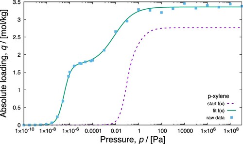
8.5. Examples

RUPTURA comes with many examples included. These examples have three parts: (1) fitting the pure component isotherm data with different isotherm models to obtain isotherm parameters (e.g. equilibrium constant (b), saturation loading , etc), (2) prediction of mixture isotherms with the fitted parameters as input, (3) breakthrough curve simulations with the fitted parameters as input. The examples range from a simple binary mixture up to a 15-component C${}_5$-C${}_6$-C${}_7$ alkane mixture. The xylene-examples have been selecting for displaying qualitatively different adsorption behaviour.

The examples are listed in Table 14 along with typical run times for breakthrough simulations, here on a mac-studio using an M1-chip. Most examples run in a few minutes. However, keep in mind that run-times depend on the total pressure. Increasing the pressure shifts the breakthrough to shorter dimensionless times, decreasing the pressure shifts the breakthrough to longer dimensionless times. Also, for lower pressure or stiff systems, a smaller time-step might be in order. This could significantly increase the computational time needed for the breakthrough computation. Other factors that influence the run times are the details of the isotherm models and isotherm shapes.

Table 14. List of mixture prediction, breakthrough, and fitting examples provided with RUPTURA.

structure	mixture	$N_{{}_C}$	$N_{\mathrm{g}\mathrm{r}\mathrm{i}\mathrm{d}}$	$\mathrm{\Delta }t$ [s]	$p_i$ [kPa]	$\tau =tv/L$ [−]	time	$p_i$ [kPa]	$\tau =tv/L$ [−]	time
MOR	CO${}_2$-C${}_3$H${}_8$	2	100	0.0005	125.0	270.8	1m36	1250.0	53.2	0m25
JUC-77	xylenes	4	100	0.0005	25.0	201.8	4m02	250.0	43.5	0m58
MIL-125-NH2	xylenes	4	100	0.0005	25.0	355.5	7m34	250.0	77.2	2m07
CoBDP	xylenes	4	100	0.0005	25.0	395.3	8m08	250.0	68.5	1m50
MFI	xylenes	4	100	0.0005	25.0	1025.2	10m13	250.0	162.5	2m08
MIL-47	xylenes	4	100	0.0005	25.0	504.5	11m18	250.0	95.0	2m37
MAF-X8	xylenes	4	100	0.0005	25.0	643.2	13m28	250.0	99.0	2m37
CoBDP	alkanes-C${}_6$	5	100	0.0005	20.0	489.3	13m33	200.0	86.2	2m51
BEA	alkanes-C${}_7$	5	100	0.0005	1.2	873.24	17m10	12.0	331.7	6m57
fe2bdp3	alkanes-C${}_6$	5	100	0.0005	20.0	3520.0	105m58	200.0	376.7	12m41
ZIF-77	alkanes-C${}_5$-C${}_6$-C${}_7$	15	100	0.0005	20.0	269.3	28m03	200.0	52.8	5m44

Notes: For breakthrough simulations, in addition to the $N_{{}_C}$-components, there is a carrier-gas component present. The timings are done on a mac-studio using an M1-chip.

9. RUPTURA troubleshooting

9.1. The curve fitting does not visually match well to the isotherm data

Run the fitting several times to make sure the solution is stable. If the problem remains, then it is the isotherm model and/or the number of isotherm sites. Increase the number of sites if inflections are not represented well.

9.2. Breakthrough error: pressure gradient is too large (negative outlet pressure)

The given pressure and pressure gradient result in negative pressure further down the column. This is nonphysical and indicates that the pressure gradient is chosen too high, and/or the pressure is too low.

9.3. Instability or erratic breakthrough curves

The time step might be too high, reduce the time step and check for improvement. Check the values of mass transfer and axial dispersion coefficients for physical validity. Check whether using the reference IAS method using bisection (IASTMethod Bisection) makes a difference. Try this first in a mixture prediction calculation, since this is fast. If you find a difference, then there is a numerical instability in the implemented FastIAS method.

9.4. Breakthrough curves with sharp transitions or spikes

Use more grid points in the spatial discretisation of the column.

9.5. The breakthrough curve depends on the time-step and number of grid points

The breakthrough curves are correct in the limit of a very small time-step and a large number of grid points. Generally, you will have to chooses the time-step and number of grid points such that a further decrease in time-step or increase in number of grid points will not (visually) change the breakthrough curves anymore. Note that always using a very small time-step and a large amount of grid points is computationally expensive.

9.6. No convergence or hangs

Use recommended units, like mol/kg for loading, and Pascal for pressure. Other units could lead to very small or very large numbers.

10. Conclusions

We presented the RUPTURA code (https://github.com/iraspa/ruptura), which is a freely available, open-source package for the computation of breakthrough curves, mixture adsorption, and fitting of isotherm models to raw adsorption data. RUPTURA contains three modules of workflow encountered in this field: (1) the computation of step/pulse breakthrough, (2) the prediction of mixture adsorption (used in the breakthrough equations) based on pure component isotherms, and (3) the fitting of isotherm models on raw (computed or measured) isotherm data. We included isotherm models like Langmuir, BET, Henry, Freundlich, Sips, Langmuir-Freundlich, Redlich-Peterson, Toth, Unilan, O'Brian & Myers, Asymptotic Temkin, and Bingel & Walton including their multi-site versions or combinations of that. The mixture prediction methods implemented include Ideal Adsorption Solution Theory (IAST), segregated IAST, and explicit Langmuir methods. IAST is computed fast and at machine precision. The breakthrough simulations include axial dispersion and the Linear Driving Force (LDF) model for mass-transfer, and have excellent numerical stability through the use of Strong-Stability Preserving Runge-Kutta (SSP-RK) integrators. RUPTURA is freely available (MIT license) and should be viewed as a demonstration ‘code’ that could be useful for researchers working in the field and for teaching in chemistry and chemical engineering classes. For future versions of RUPTURA, we envision to include support for non-ideal gas behaviour, liquid phase conditions, and chemical reactions. Non-isothermal operation is an important aspect that needs to be considered. Variation in temperature along the column can be significant for certain cases such as adsorption of CO${}_2$. Therefore, in the next version of RUPTURA, we plan to include non-isothermal operation. Also, the code will be modified for simulating adsorption columns with more than one type of adsorbent. This will be useful in separating multiple components inside the column.

Acknowledgments

We are thankful to C3UPO for the provided HPC facilities. The authors acknowledge the use of computational resources of DelftBlue supercomputer, provided by Delft High Performance Computing Centre (https://www.tudelft.nl/dhpc).

Disclosure statement

No potential conflict of interest was reported by the author(s).

Additional information

Funding

This work was sponsored by NWO Domain Science for the use of supercomputer facilities. This work is part of the Advanced Research Center for Chemical Building Blocks, ARC-CBBC, which is co-funded and co-financed by the Netherlands Organisation for Scientific Research (NWO) and the Netherlands Ministry of Economic Affairs and Climate Policy. SRGB was supported with Grant POSTDOC_21_00069 funded by Consejería de Transformación Económica, Industria, Conocimiento y Universidades and Agencia Andaluza del Conocimiento, Junta de Andalucía.

References

- de Haan A, Bosch H. Industrial separation processes; fundamentals. Berlin/Boston: De Gruyter; 2013.
- Pullumbi P, Brandani F, Brandani S. Gas separation by adsorption: technological drivers and opportunities for improvement. Curr Opin Chem Eng. 2019;24:131–142.
- Yu C, Huang C, Tan C. A review of CO2 capture by absorption and adsorption. Aerosol Air Qual Res. 2012;12:745–769.
- Jiuhui Q. Research progress of novel adsorption processes in water purification: a review. J Environ Sci. 2008;20:1–13.
- Alghoul M, Sulaiman M, Azmi B, et al. Review of materials for adsorption refrigeration technology. Anti-Corros Method M. 2007;54:225–229.
- Ruthven D. Principles of adsorption & adsorption processes. New York: John Wiley & Sons, Inc.; 1984.
- Rodrigues AE. Simulated moving bed technology: principles, design and process applications. Kidlington: Butterworth-Heinemann; 2015.
- Jiang N, Shen Y, Liu B, et al. CO
2 capture from dry flue gas by means of VPSA, TSA and TVSA. J CO
- Luis P. Chapter 8 -- hybrid processes based on membrane technology. In: Luis P, editor. Fundamental modelling of membrane systems. Amsterdam: Elsevier; 2018. p. 301–343.
- Ruthven D, Farooq S, Knaebel K. Pressure swing adsorption. New York: VCH Publishers Inc.; 1994.
- Canevesi R, Borba C, da Silva A, et al. Towards a design of a pressure swing adsorption unit for small scale biogas upgrading at. Energy Procedia. 2019;158:848–853.
- Yavary M, Ebrahim H, Falamaki C. The effect of number of pressure equalization steps on the performance of pressure swing adsorption process. Chem Eng Process. 2015;87:35–44.
- Grande C. Advances in pressure swing adsorption for gas separation. Int Schol Res Not. 2012;2012:982934.
- Oschatz M, Antonietti M. A search for selectivity to enable CO 2 capture with porous adsorbents. Energy Environ Sci. 2018;11:57–70.
- Kumar R. Pressure swing adsorption process: performance optimum and adsorbent selection. Ind Eng Chem Res. 1994;33:1600–1605.
- Ho M, Allinson G, Wiley D. Reducing the cost of CO 2 capture from flue gases using pressure swing adsorption. Ind Eng Chem Res. 2008;47:4883–4890.
- Bhatia S, Myers A. Optimum conditions for adsorptive storage. Langmuir. 2006;22:1688–1700.
- Al Mohammed M, Danish M, Khan I, et al. Continuous fixed bed CO 2 adsorption: breakthrough, column efficiency, mass transfer zone. Processes. 2020;8:1233.
- Rodrigues AE. Perspectives on adsorption. what else? a personal view. Fluid Phase Equilib. 2023;564:Article ID 113614.
- Tien C. Introduction to adsorption: basics, analysis, and applications. Amsterdam: Elsevier; 2019.
- Dubbeldam D, Calero S, Ellis DE, et al. RASPA: molecular simulation software for adsorption and diffusion in flexible nanoporous materials. Mol Simul. 2016;42(2):81–101.
- Dubbeldam D, Torres-Knoop A, Walton KS. On the inner workings of Monte Carlo codes. Mol Simul. 2013;39(14–15):1253–1292.
- Do D. Adsorption analysis: equilbria and kinetics. London: Imperial College Press; 1998.
- Guiochon G, Felinger A, Shirazi D. Fundamentals of preparative and nonlinear chromatography. 2nd ed. Amsterdam: Academic Press; 2006.
- Moradi O. Thermodynamics of interfaces. book section 8. Rijeka: InTechOpen; 2011.
- Ayawei N, Ebelegi A, Wankasi D. Modelling and interpretation of adsorption isotherms. J Chem. 2017;2017:Article ID 3039817.
- Girish C. Various isotherm models for multicomponent adsorption: a review. Int J Res Civ Eng Technol. 2017;8:80–86.
- Myers A, Prausnitz J. Thermodynamics of mixed-gas adsorption. AIChE J. 1965;11:121–127.
- Swisher J, Lin L-C, Kim J, et al. Evaluating mixture adsorption models using molecular simulation. AIChE J. 2013;59:3054–3064.
- Van Assche T, Baron G, Denayer J. An explicit multicomponent adsorption isotherm model: accounting for the size-effect for components with Langmuir adsorption behavior. Adsorption. 2018;24:517–530.
- Sharma S, Rigutto M, Baur R, et al. Modelling of adsorbate-size dependent explicit isotherms using a segregated approach to account for surface heterogeneities. Mol Phys. In press. 2023. DOI:10.1080/00268976.2023.2183721.
- Glueckauf E. Theory of chromatography part 10. formulae for diffusion into spheres and their application to chromatography. T Faraday Soc. 1955;51:1540–1551.
- Shu C-W. Total-variation diminishing time discretizations. IAM J Sci Statist Comput. 1988;9:1073–1084.
- Shu C, Osher S. Efficient implementation of essentially non-oscillatory shock-capturing schemes. J Comput Phys. 1988;77:439–471.
- Gottlieb S, Gottlieb L. Strong stability preserving properties of runge-kutta time discretization methods for linear constant coefficient operators. J Sci Comput. 2003;18:83–109.
- Ketcheson D. Highly efficient strong stability-preserving Runge-Kutta methods with low-storage implementations. SIAM J Sci Comput. 2008;30:2113–2136.
- Landa H. Development of an efficient method for simulating fixed-bed adsorption dynamics using Ideal Adsorbed Solution Theory [PhD thesis]. Otto-von-Guericke-Universität Magdeburg. 2016. Available from: http://d-nb.info/1128726513/34.
- Winterton R. Van der Waals forces. Contemp Phys. 1970;11:559–574.
- Condon J. Surface area and porosity determinations by physisorption: measurements and theory. Amsterdam: Elsevier Science; 2006.
- Dabrowski A. Adsorption -- from theory to practice. Adv Colloid Interface Sci. 2001;93:135–224.
- Sircar S. Excess properties and thermodynamics of multicomponent gas adsorption. J Chem Soc Faraday Trans 1 F. 1985;81:1527–1540.
- Pini R. Interpretation of net and excess adsorption isotherms in microporous adsorbents. Microporous Mesoporous Mater. 2014;187:40–52.
- Gumma S, Talu O. Net adsorption: A thermodynamic framework for supercritical gas adsorption and storage in porous solids. Langmuir. 2010;26:17013–17023.
- Myers A. Thermodynamics of adsorption in porous materials. AIChE J. 2002;48:145–160.
- Bingel L, Walton K. Surprising use of the business innovation bass diffusion model to accurately describe adsorption isotherm types I, III, and V. Langmuir. 2023;39:4475–4482.
- Langmuir I. The adsorption of gases on plane surfaces of glass, mica and platinum. J Am Chem Soc. 1918;40:1361–1403.
- Gritti F, Guiochon G. New thermodynamically consistent competitive adsorption isotherm in RPLC. J Colloid Interface Sci. 2003;1:43–59.
- Boedeker C. Über das verhältnis zwischen masse und wirkung beim kontakt ammoniakalscher flüssigkeiten mit ackererde und mit kohlensaurem kalk. ZA Pflanzenbau. 1859;7:48–58.
- Sips R. On the structure of a catalyst surface. J Chem Phys. 1948;16:490–495.
- Koble R, Corrigan T. Adsorption isotherms for pure hydrocarbons. Ind Eng Chem Res. 1952;44:383–387.
- Redlich O, Peterson D. A useful adsorption isotherm. J Phys Chem. 1959;63:1024.
- Toth J. State equations of the solid-gas interface layers. Acta Chim Acad Sci Hung. 1971;69:311–328.
- Toth J. Uniform interpretation of gas/solid adsorption. Adv Colloid Interface Sci. 1995;55:1–239.
- Toth J. Adsorption: theory, modelling, and analysis. New York: Marcel Dekker Inc; 2002.
- O'Brien JA, Myers AL. Physical adsorption of gases on heterogeneous surfaces: series expansion of isotherms using central moments of the adsorption energy distribution. J Chem Soc Faraday Trans. 1984;80:1467–1477.
- Hill T. An introduction to statistical thermodynamics. New York: Dover Publications; 1986.
- Lin B, Ma Z, Golshan-Shirazi S, et al. Study of the representation of competitive isotherms and of the intersection between adsorption isotherms. J Chromatogr. 1989;475:1–11.
- Tempkin V. Kinetics of ammonia synthesis on promoted iron catalyst. Acta Phys Chim USSR. 1940;12:327–356.
- Simon C, Kim J, Lin L-C, et al. Optimizing nanoporous materials for gas storage. Phys Chem Chem Phys. 2014;16:5499–5513.
- Graham D. The characterization of physical adsorption systems. J Phys Chem. 1953;57:665–669.
- Smit B, Maesen T. Commensurate freezing of alkanes in the channels of a zeolite. Nature. 1995;374:42–44.
- Vlugt TJH, Krishna R, Smit B. Molecular simulations of adsorption isotherms for linear and branched alkanes and their mixtures in silicalite. J Phys Chem B. 1999;103:1102–1118.
- Tarafder A, Mazzotti M. A method for deriving explicit binary isotherms obeying the ideal adsorbed solution theory. Chem Eng Technol. 2012;35:102–108.
- Worch E. Adsorption technology in water treatment. Berlin/Boston: Walter de Gruyter GmbH & Co; 2012.
- Weber Jr W, DiGiano F. Process dynamics in environmental systems. New York: John Wiley & Sons; 1996.
- Talu O, Myers A. Rigorous thermodynamic treatment of gas adsorption. AIChE J. 1988;34:1887–1893.
- Bass F. A new product growth for model consumer durables. Manag Sci. 1969;15:215–227.
- DeVoe H. Thermodynamics and chemistry. Hoboken: Prentice-Hall, Inc.; 2015.
- Myers A, Monson P. Physical adsorption of gases: the case for absolute adsorption as the basis for thermodynamic analysis. Adsorption. 2014;20:591–622.
- Murthi M, Snurr R. Effects of molecular siting and adsorbent heterogeneity on the ideality of adsorption equilibria. Langmuir. 2004;20:2489–2497.
- Brandani S, Mangano E, Luberti M. Net, excess, and absolute adsorption in mixed gas adsorption. Adsorption. 2017;23:569–576.
- Myers A. Thermodynamics of adsorption. In: Letcher T, editor. Chemical thermodynamics for industry. chapter 21. Cambridge: Royal Society of Chemistry; 2004. p. 243–253.
- Santori G, Luberti M, Ahn H. Ideal adsorbed solution theory solved with direct search minimisation. Comput Chem Eng. 2014;71:235–240.
- Landa H, Flockerzi D, Seidel-Morgenstern A. A method for efficiently solving the IAST equations with an application to adsorber dynamics. AIChE J. 2012;59:1263–1277.
- Seidel A, Reschke G, Friedrich S, et al. Equilibrium adsorption of two-component organic solutes from aqueous solutions on activated carbon. Adsorption Sci Technol. 1986;3:189–199.
- Myers A, Valenzuela D. Adsorption from bisolute systems on active carbon. J Water Pollut Control Fed. 1973;45:2463–2479.
- Simon C, Smit B, Haranczyk M. pyIAST: ideal adsorbed solution theory (IAST) python package. Comput Phys Commun. 2016;200:364–380.
- Voigt A. Comparison of methods for the calculation of the real dilogarithm regarding instruction-level parallelism. arXiv:2201.01678. 2022.
- Vidunas R. Algebraic transformations of gauss hypergeometric functions. Funkcial Ekvac. 2009;52:139–180.
- Koepf W. Gosper's algorithm. London: Springer London; 2014. p. 79–101.
- Shade D, Bout B, Sholl D, et al. Opening the toolbox: 18 experimental techniques for measurement of mixed gas adsorption. Ind Eng Chem Res. 2022;61:2367–2391.
- Walton K, Sholl D. Predicting multicomponent adsorption: 50 years of the ideal adsorbed solution theory. AIChE J. 2015;61:2757–2762.
- Frenkel D, Smit B. Understanding molecular simulation: from algorithms to applications. 2nd ed. Orlando: Elsevier; 2001.
- Butler J, Ockrent C. Studies in electrocapillarity. Part III. The surface tensions of solutions containing two surface-active solutes. J Phys Chem. 1930;34:2841–2859.
- Broughton D. Adsorption isotherms for binary gas mixtures. Ind Eng Chem. 1948;40:1506–1508.
- Jain J, Snoeyink V. Adsorption from bisolute systems on active carbon. J Water Pollut Control Fed. 1973;45:2463–2479.
- Yang R. Adsorbents: fundamentals and applications. Hoboken: John Wiley & Sons; 2003.
- O'Brien J, Myers A. Rapid calculations of multicomponent adsorption equilibria from pure isotherm data. Ind Eng Chem Process Des Dev. 1985;24:1188–1191.
- Chen H, Sholl D. Examining the accuracy of ideal adsorbed solution theory without curve-fitting using transition matrix monte carlo simulations. Langmuir. 2007;23:6431–6437.
- Cessford N, Seaton N, Düren T. Evaluation of ideal adsorbed solution theory as a tool for the design of metal–organic framework materials. Ind Eng Chem Res. 2012;51:4911–4921.
- Krishna R, van Baten J. How reliable is the ideal adsorbed solution theory for the estimation of mixture separation selectivities in microporous crystalline adsorbents?. ACS Omega. 2021;6:15499–15513.
- Fraux G, Boutin A, Coudert F-X. On the use of the IAST method for gas separation studies in porous materials with gate-opening behavior. Adsorption. 2018;24:233–241.
- Gharagheizi F, Sholl D. Comprehensive assessment of the accuracy of the ideal adsorbed solution theory for predicting binary adsorption of gas mixtures in porous materials. Ind Eng Chem Res. 2022;61:727–739.
- Suwanayuen S, Danner RP. Vacancy solution theory of adsorption from gas mixtures. AIChE J. 1980;26:76–83.
- Costa E, Sotelo J, Calleja G, et al. Adsorption of binary and ternary hydrocarbon-gas mixtures on activated carbon -- experimental-determination and theoretical prediction of the ternary equilibrium data. AIChE J. 1981;27:5–12.
- Gamba G, Rota R, Storti G, et al. Vacancy solution theory of adsorption from gas mixtures. AIChE J. 1989;35:959–966.
- Talu O, Zwiebel I. Multicomponent adsorption equilibria of nonideal mixtures. AIChE J. 1986;32:1263–1276.
- Sakuth M, Meyer J, Gmehling J. Measurement and prediction of binary adsorption equilibria of vapors on dealuminated Y-zeolites (DAY). Chem Eng Process. 1998;37:267–277.
- Bartholdy S, Bjorner MG, Solbraa E, et al. Measurement and prediction of binary adsorption equilibria of vapors on dealuminated Y-zeolites (DAY). Ind Eng Chem Res. 2013;52:11552–11563.
- Ladshaw A, Yiacoumi S, Tsouris C. A generalized procedure for the prediction of multicomponent adsorption. AIChE J. 2015;61:2600–2610.
- Smith J, van Ness H. Introduction to chemical engineering thermodynamics. 4th ed. New York: McGraw-Hill; 1987.
- Radke CJ, Prausnitz J. Thermodynamics of multi-solute adsorption from dilute liquid solutions. AIChE J. 1972;18:761–768.
- Richter E, Schutz W, Myers A. Effect of adsorption equation on prediction of multicomponent adsorption equilibria by the ideal adsorbed solution theory. Chem Eng Sci. 1989;22:1609–1616.
- Myers AL, Valenzuela D. Computer algorithm and graphical method for calculating adsorption equilibria of gas mixtures. J Chem Eng Jpn. 1986;19:392–396.
- LeVan M, Vermeulen T. Binary langmuir and freundlich isotherms for ideal adsorbed solutions. J Phys Chem. 1981;85:3247–3250.
- Ilic M, Flockerzi D, Seidel-Morgenstern A. A thermodynamically consistent explicit competitive adsorption isotherm model based on second-order single component behaviour. J Chromatogr A. 2010;1217:2132–2137.
- Cardano G, Witmer T. The great art; or, the rules of algebra. translated and edited by T. Richard Witmer. Cambridge: MIT Press; 1968.
- Van Assche T, Baron G, Denayer J. Adsorption size effects for Langmuir systems in process simulators: case study comparing explicit Langmuir-based models and FASTIAS. Ind Eng Chem Res. 2021;60:12092–12099.
- Poursaeidesfahani A, Andres-Garcia E, de Lange M, et al. Prediction of adsorption isotherms from breakthrough curves. Microporous Mesoporous Mater. 2019;277:237–244.
- Moon H, Tien C. Further work on multicomponent adsorption equilibria calculations based on the ideal adsorbed solution theory. Ind Eng Chem Res. 1987;26:2042–2047.
- Yun JH, Park HC, Moon H. Multicomponent adsorption calculations based on adsorbed solution theory. Korean J Chem Eng. 1996;13:246–254.
- Mangano E, Friedrich D, Brandani S. Robust algorithms for the solution of the ideal adsorbed solution theory equations. AIChE J. 2014;61:981–991.
- O'Brien J, Myers A. A comprehensive technique for equilibrium calculations in adsorbed mixtures: the generalized FastIAS method. Ind Eng Chem Res. 1988;27:2085–2092.
- Choy K, Porter J, McKay G. Single and multicomponent equilibrium studies for the adsorption of acidic dyes on carbon from effluent. Langmuir. 2004;20:9646–9656.
- Frey D, Rodrigues A. Explicit calculation of multicomponent equilibria for ideal adsorbed solutions. AIChE J. 1994;40:182–186.
- Santos J, Cheng Y, Dias M, et al. Surface B-splines fitting for speeding up the simulation of adsorption processes with IAS model. Comput Chem Eng. 2011;35:1186–1191.
- Nelder J, Mead R. A simplex method for function minimization. Comput J. 1965;7:308–313.
- Mirzaei A, Chen Z, Haghighat F, et al. Enhanced adsorption of anionic dyes by surface fluorination of zinc oxide: A straightforward method for numerical solving of the ideal adsorbed solution theory (IAST). Chem Eng J. 2017;30:407–418.
- Benjamin M. New conceptualization and solution approach for the ideal adsorbed solution theory (IAST). Environ Sci Technol. 2009;43:2530–2536.
- Balestra S, Bueno-Perez R, Aguilar R, et al. GAIAST: a fortran code with genetic algorithms (GA) for an adsorbed solution theory (IAST). 2016. DOI:10.5281/zenodo.596674.
- Lee S, Lee JH, Kim J. User-friendly graphical user interface software for ideal adsorbed solution theory calculations. Korean J Chem Eng. 2018;35:214–221.
- Iacomi P, Llewellyn P. pyGAPS: a python-based framework for adsorption isotherm processing and material characterisation. Adsorption. 2019;25:1533–1542.
- Dautzenberg E, Smulders M, de Smet LCPM. Graphiast: A graphical user interface software for ideal adsorption solution theory (IAST) calculations. Comput Phys Commun. 2022;280:Article ID 108494.
- Hoseinpoori S. Steady-state modeling of co-adsorption phenomena in direct air carbon-capture system using the IAST [Thesis]. Politecnico di Milano and RWTH Aachen University. 2020. Available from: http://hdl.handle.net/10589/169486.
- Chabert J, Barbin E, Borowczyk J, et al. A history of algorithms: from the pebble to the microchip. Berlin, Heidelberg, New York: Springer; 1999.
- Dynamic sorption methods. Nov 2022. Available from: https://www.dynamicsorption.com/dynamic-sorption-method/.
- Patel H. Fixed-bed column adsorption study: a comprehensive review. Appl Water Sci. 2019;9:1–17.
- Silva J, Ferreira A, Mendes P, et al. Adsorption equilibrium and dynamics of fixed bed adsorption of CH 4/N 2 in binderless beads of 5A zeolite. Ind Eng Chem Res. 2015;54:6390–6399.
- Wilkins N, Rajendran A, Farooq S. Dynamic column breakthrough experiments for measurement of adsorption equilibrium and kinetics. Adsorption. 2021;27:397–422.
- Farmahini A, Krishnamurthy S, Friedrich D, et al. Performance-based screening of porous materials for carbon capture. Chem Rev. 2021;121:10666–10741.
- Gabelman A. Adsorption basics: part 1. Chem Eng Prog. 2017;113:48–53.
- Klaewkla R, Arend M, Hoelderich W. A review of mass transfer controlling the reaction rate in heterogeneous catalytic systems. In: Nakajima H., editor. Mass transfer-advanced aspects. chapter 29. London: INTECH Open Access Publisher; 2011.
- Fogler H. Elements of chemical reaction in engineering. 3th ed. Naucalpan de Juárez: Prentice-Hall of India; 1999.
- Xu Z, Cai J-G, Pan B-C. Mathematically modeling fixed-bed adsorption in aqueous systems. J Zhejiang Univ Sci A. 2013;14:155–176.
- Jee J, Park H, Haam S, et al. Effects of nonisobaric and isobaric steps on o2 pressure swing adsorption for an aerator. Ind Eng Chem Res. 2002;41:4383–4392.
- Kim M, Moon J, Lee C, et al. Effect of heat transfer on the transient dynamics of temperature swing adsorption process. Korean J Chem Eng. 2004;21:703–711.
- Shafeeyan M, Daud W, Shamiri A. A review of mathematical modeling of fixed-bed columns for carbon dioxide adsorption. Chem Eng Res Des. 2014;92:961–988.
- Sircar S, Hufton J. Why does the linear driving force model for adsorption kinetics work?. Adsorption. 2000;6:137–147.
- Hwang K, Jun J, Lee W. Fixed-bed adsorption for bulk component system non-equilibrium, non-isothermal and non-adiabatic model. Chem Eng Sci. 1995;50:813–825.
- Tien C. Adsorption calculations and modeling. Boston: Butterworth-Heinemann; 1994.
- Worch E. Fixed-bed adsorption in drinking water treatment: a critical review on models and parameter estimation. J Water Supply Res Technol AQUA. 2008;57:171–183.
- Siahpoosh M, Fatemi S, Vatani A. Mathematical modeling of single and multi-component adsorption fixed beds to rigorously predict the mass transfer zone and breakthrough curves. Iran J Chem Chem Eng. 2009;28:25–44.
- Supian NM, Halif NA, Rusli N. A mini-review of coupled convection-diffusion equations in a fixed-bed adsorption. IOP Conf Ser Mater Sci Eng. 2019;767:Article ID 012031.
- Unuabonah E, Omorogie M, Oladoja N. 5 -- modeling in adsorption: fundamentals and applications. Amsterdam: Elsevier; 2019. p. 85–118.
- Yang R. Gas separation by adsorption processes. London: Imperial College Press; 1987.
- Thomas H. Heterogeneous ion exchange in a flowing system. J Am Chem Soc. 1944;66:1664–1666.
- Bohart G, Adams E. Some aspects of the behavior of charcoal with respect to chlorine. J Am Chem Soc. 1920;42:523–544.
- Yoon Y, Nelson J. Application of gas adsorption kinetics I. a theoretical model for respirator cartridge service life. Am Ind Hyg Assoc J. 1984;45:509–516.
- Unuabonah E, El-Khaiary M, Olu-Owolabi B, et al. Predicting the dynamics and performance of a polymer–clay based composite in a fixed bed system for the removal of lead (II) ion. Chem Eng Res Des. 2012;90:1105–1115.
- Clark R. Evaluating the cost and performance of field-scale granular activated carbon systems. Environ Sci Technol. 1987;21:573–580.
- Lapidus L, Amundson N. The effect of longitudinal diffusion in ion exchange and chromatographic columns. J Phys Chem. 1952;56:984–988.
- Plazinski W, Rudzinskia W, Plazinska A. Theoretical models of sorption kinetics including a surface reaction mechanism: A review. Adv Colloid Interface Sci. 2009;152:2–13.
- Medved I, Cerny R. Surface diffusion in porous media: A critical review. Microporous Mesoporous Mater. 2011;142:405–422.
- Fick A. Ueber diffusion. Ann Phys. 1855;170:59–86.
- Knox J. Predictive simulation of gas adsorption in fixed-beds and limitations due to the ill-posed danckwerts boundary condition [Thesis]. Swiss School of Business Research. 2016. Available from: https://louis.uah.edu/uah-dissertations/108/.
- de Ligny C. Coupling between diffusion and convection in radial dispersion of matter by fluid flow through packed beds. Chem Eng Sci. 1970;25:1177–1181.
- Chung S, Wen C. Longitudinal dispersion of liquid flowing through fixed and fluidized beds. AIChE J. 1968;14:857–866.
- Rastegar S, Gu T. Empirical correlations for axial dispersion coefficient and Peclet number in fixed-bed columns. J Chromatogr A. 2017;1490:133–137.
- Edward M, Richardson J. Gas dispersion in packed beds. Chem Eng Sci. 1968;23:109–123.
- da Silva F, Silva J, Rodrigues A. A general package for the simulation of cyclic adsorption processes. Adsorption. 1999;5:229–244.
- Tsimpanogiannis I, Moultos O, Franco L, et al. Self-diffusion coefficient of bulk and confined water: a critical review of classical molecular simulation studies. Mol Simul. 2019;45:425–453.
- Celebi A, Jamali S, Bardow A, et al. Finite-size effects of diffusion coefficients computed from molecular dynamics: a review of what we have learned so far. Mol Simul. 2021;47:831–845.
- Cussler E. Diffusion: mass transfer in fluid systems. New York: Cambridge University Press; 2009.
- Bird R. Transport phenomena. Appl Mech Rev. 2002;55:R1–R4.
- Jones J. On the determination of molecular fields.–I. from the variation of the viscosity of a gas with temperature. Proc R Soc Lond Ser A-Contain Pap Math Phys Char. 1924a;106:441–462.
- Jones J. On the determination of molecular fields.–II. from the equation of state of a gas. Proc R Soc Lond Ser A-Contain Pap Math Phys Char. 1924b;106:463–477.
- Kärger J, Ruthven D, Theodorou D. Diffusion in nanoporous materials. Weinheim: John Wiley & Sons; 2012.
- Crittenden J, Hutzler N, Geyer D, et al. Transport of organic compounds with saturated groundwater flow: model development and parameter sensitivity. Water Resour Res. 1986;22:271–284.
- Kapoor A, Yang R, Wong C. Surface-diffusion. Catal Rev Sci Eng. 1989;31:129–214.
- Rosen J. Kinetics of a fixed bed system for solid diffusion into spherical particles. J Chem Phys. 1952;20:387–394.
- Mathews A, Weber Jr W. Effects of external mass transfer and intraparticle diffusion on adsorption in slurry reactors. AIChE Symp Ser. 1976;73:91–98.
- Peel R, Benedek A, Crowe C. A branched pore kinetic-model for activated carbon adsorption. AIChE J. 1981;27:26–32.
- Zhang S, Sun Y. Study on protein adsorption kinetics to a dye–ligand adsorbent by the pore diffusion model. J Chromatogr A. 2002;964:35–46.
- Ko D, Porter J, McKay G. Film-pore diffusion model for the fixed-bed sorption of copper and cadmium ions onto bone char. Water Res. 2001;35:3876–3886.
- Worch E. Modelling the solute transport under nonequilibrium conditions on the basis of mass transfer equations. J Contam Hydrol. 2004;68:97–120.
- Rahman M, Amiri F, Worch E. Application of the mass transfer model for describing non-equilibrium transport of HOCs through natural geosorbents. Water Res. 2003;37:4673–4684.
- Weber T, Chakravorti R. Pore and solid diffusion models for fixed-bed adsorbers. AIChE J. 1974;20:228–238.
- Spahn H, Schlunder E. The scale-up of activated carbon columns for water purification, based on results from batch tests–I: theoretical and experimental determination of adsorption rates of single organic solutes in batch tests. Chem Eng Sci. 1975;30:529–537.
- Brauch V, Schlunder E. The scale-up of activated carbon columns for water purification, based on results from batch tests–II: theoretical and experimental determination of breakthrough curves in activated carbon columns. Chem Eng Sci. 1975;30:539–548.
- Levenspiel O. Chemical reaction engineering. Ind Eng Chem Res. 1999;38:4140–4143.
- Yang X, Otto S, Al-Duri B. Concentration-dependent surface diffusivity model (CDSDM): numerical development and application. Chem Eng J. 2003;94:199–209.
- Rudin A, Choi P. The elements of polymer science and engineering: an introductory text for engineers and chemists. 3th ed. Oxford: Academic Press; 2012.
- Kooijman H, Taylor R. Estimation of diffusion-coefficients in multicomponent liquid-systems. Ind Eng Chem Res. 1991;30:1217–1222.
- Theodorou D, Snurr R, Bell A. Molecular dynamics and diffusion in microporous materials. In Alberti G and Bein T, editors. Comprehensive Supramolecular Chemistry. Vol. 7, chapter 18. Oxford: Pergamon Oxford; 1996. p. 507–548.
- Krishna R. Diffusion in porous crystalline materials. Chem Soc Rev. 2012;41:3099–3118.
- Krishna R, Taylor R. Multicomponent mass transfer-theory and applications. chapter 7. Houston: Gulf PublishingCo.; 1986.
- Krishna R, Baur R. Modelling issues in zeolite based separation processes. Sep Purif Technol. 2003;33:213–254.
- Ramanan H, Auerbach S. Molecular dynamics and diffusion in microporous materials. In: Conner WC and Fraissard J, editors. Fluid Transport in Nanoporous Materials. Proceedings of the NATO Advanced Study Institute. Dordrecht: Springer; 2006. p. 93–124.
- Krishna R, van Baten J. Describing binary mixture diffusion in carbon nanotubes with the Maxwell-Stefan equations. an investigation using molecular dynamics simulations. Ind Eng Chem Res. 2006;45:2084–2093.
- Dubbeldam D, Snurr R. Recent developments in the molecular modeling of diffusion in nanoporous materials. Mol Simul. 2007;33:305–325.
- Valkovska D, Danov K. Determination of bulk and surface diffusion coefficients from experimental data for thin liquid film drainage. J Colloid Interface Sci. 2000;223:314–316.
- LeVan M, Carta G, Carmen M. Adsorption and ion exchange. In: Perry R. and Green D, editors. Perry's chemical engineers' handbook. New York: McGraw-Hill; 2008.
- Hand D, Crittenden J, Thacker W. Simplified models for design of fixed-bed adsorption systems. J Environ Eng. 1984;110:440–456.
- Baup S, Jaffre C, Wolbert D, et al. Adsorption of pesticides onto granular activated carbon: determination of surface diffusivities using simple batch experiments. Adsorption. 2000;6:219–228.
- Ozdural A. 2.51 -- modeling chromatographic separation. 3rd ed. Oxford: Pergamon; 2017. p. 754–772.
- Al-Duri B. Adsorption modelling and mass transfer. In: McKay G, editor. Use of adsorbents for the removal of pollutants from wastewaters. Boca Raton: CRC Press; 1996. p. 133–173.
- Liaw C, Wang J, Greenkorn R, et al. Kinetics of fixed-bed adsorption -- new solution. AIChE J. 1979;25:376–381.
- Alvarez-Ramirez J, Fernandez-Anaya G, Valdes-Parada F, et al. Physical consistency of generalized linear driving force models for adsorption in a particle. Ind Eng Chem Res. 2005;44:6776–6783.
- Krishna R. A Maxwell-Stefan-Glueckauf description of transient mixture uptake in microporous adsorbents. Sep Purif Technol. 2018;191:392–399.
- Mota J, Rodrigo A. Calculations of multicomponent adsorption-column dynamics combining the potential and ideal adsorbed solution theories. Ind Eng Chem Res. 2000;39:2459–2467.
- Sperlich A, Schimmelpfennig S, Baumgarten B, et al. Predicting anion breakthrough in Granular Ferric Hydroxide (GFH) adsorption filters. Water Res. 2008;42:2073–2082.
- Bodin J. MFIT 1.0. 0: multi-flow inversion of tracer breakthrough curves in fractured and karst aquifers. Geosci Model Dev. 2020;13:2905–2924.
- Kane A, Giraudet S, Vilmain J-B, et al. Intensification of the temperature-swing adsorption process with a heat pump for the recovery of dichloromethane. J Environ Chem Eng. 2015;3:734–743.
- Möller A, Eschrich R, Reichenbach C, et al. Dynamic and equilibrium-based investigations of CO 2-removal from CH 4-rich gas mixtures on microporous adsorbents. Adsorption. 2017;23:197–209.
- Aspen Adsorption. Dec 2022. Available from: https://www.aspentech.com/en/products/pages/aspen-adsorption.
- Zhang R, Shen Y, Tang Z, et al. A review of numerical research on the pressure swing adsorption process. Processes. 2022;10:812.
- gPROMS. Dec 2022. Available from: https://www.psenterprise.com/products/gproms.
- MATLAB. Dec 2022. Available from: https://nl.mathworks.com/products/matlab.html.
- Ansys Fluent. Fluid simulation software. Dec 2022. Available from: https://www.ansys.com/products/fluids/ansys-fluent.
- Chung YG, Bai P, Haranczyk M, et al. Computational screening of nanoporous materials for hexane and heptane isomer separation. Chem Mater. 2017;29:6315–6328.
- Darcy H. Les fontaines publiques de la ville de Dijon: exposition et application des principes à suivre et des formules à employer dans les questions de distribution d'eau: ouvrage terminé par un appendice relatif aux fournitures d'eau de plusieurs villes, au filtrage des eaux et à la fabrication des tuyaux de fonte, de plomb, de tôle et de bitume. Vol. 2. Paris: V. Dalmont; 1856.
- Ergun S. Fluid flow through packed columns. Chem Eng Prog. 1952;48:89–94.
- Carman P. Fluid flow through a granular bed. Trans Inst Chem Eng Lond. 1937;15:150–156.
- Cheng A, Cheng D. Heritage and early history of the boundary element method. Eng Ana Bound Elmnts. 2005;29:268–302.
- Mott H, Green Z. On Danckwerts' boundary conditions for the plug-flow with dispersion/reaction model. Chem Eng Comm. 2015;202:739–745.
- Anderson J, Wendt J. Computational fluid dynamics. Vol. 206. Heidelberg: Springer; 1995.
- Versteeg H, Malalasekera W. An introduction to computational fluid dynamics: the finite volume method. Glasgow: Pearson education; 2007.
- Ottosen N, Petersson H. Introduction to finite element method. New York: Prentice Hall; 1996.
- Schiesser W. The numerical method of lines: integration of partial differential equations. London: Elsevier; 2012.
- Nilchan S, Pantelides C. On the optimisation of periodic adsorption processes. Adsorption. 1998;4:113–147.
- Cruz P, Santos J, Magalhães F, et al. Simulation of separation processes using finite volume method. Comput Chem Eng. 2005;30:83–98.
- Kikkinides E, Yang R. Effects of bed pressure drop on isothermal and adiabatic adsorber dynamics. Chem Eng Sci. 1993;48:1545–1555.
- Schiesser W. Computational mathematics in engineering and applied science: ODEs, DAEs, and PDEs. Boca Raton: CRC Press; 2014.
- Langtangen H, Linge S. Finite difference computing with PDEs: a modern software approach. Cham: Springer Nature; 2017.
- Butcher J. Numerical methods for ordinary differential equations. West Sussex: John Wiley & Sons; 2016.
- Iserles A. A first course in the numerical analysis of differential equations. Cambridge: Cambridge University Press; 2009.
- Press WH, Teukolsky SA, Vetterling WT, et al. Numerical recipes in fortran 90: the art of scientific computing. New York: Cambridge University Press; 1996.
- Verwer J, Sommeijer B. An implicit-explicit Runge-Kutta-Chebyshev scheme for diffusion-reaction equations. SIAM J Sci Comput. 2004;25:1824–1835.
- Deuflhard P, Hairer E, Zugck J. One-step and extrapolation methods for differential-algebraic systems. Numer Math. 1987;51:501–516.
- Butcher J. Implicit Runge-Kutta processes. Math Comput. 1964;18:50–64.
- Press W, Teukolsky S. Adaptive stepsize Runge-Kutta integration. Comput Phys. 1992;6:188–191.
- Torres-Knoop A, Dubbeldam D. Exploiting large-pore metal-organic frameworks for separations through entropic molecular mechanisms. Chem Phys Chem. 2015;16:2046–2067.
- Jolimaitre E, Ragil K, Tayakout-Fayolle M, et al. Separation of mono and dibranched hydrocarbons on silicalite. AIChE J. 2002;48:1927–1937.
- Caceci M, Cacheris W. Fitting curves to data. Byte. 1984;9:340–362.
- Motulsky H, Ransnas L. Fitting curves to data using nonlinear regression: a practical and non-mathematical review. The FASEB J. 1987;1:365–374.
- Jaraíz-Arroyo I, Martin-Calvo A, Gutiérrez-Sevillano J, et al. OCEAN: an algorithm to predict the separation of biogas using zeolites. Ind Eng Chem Res. 2020;59:7212–7223.
- Anderson R, Gómez-Gualdróna D. Deep learning combined with IAST to screen thermodynamically feasible mofs for adsorption-based separation of multiple binary mixtures. J Chem Phys. 2021;154:Article ID 234102.
- Lineweaver H, Burk D. The determination of enzyme dissociation constants. J Am Chem Soc. 1934;56:658–666.
- Dowd J, Riggs D. A comparison of estimates of michaelis-menten kinetic constants from various linear transformations. J Biol Chem. 1965;240:863–869.
- Eadie G. The inhibition of cholinesterase by physostigmine and prostigmine. J Bio Chem. 1942;146:85–93.
- Hofstee B. Non-inverted versus inverted plots in enzyme kinetics. Nature. 1959;184:1296–1298.
- Scatchard G. The attractions of proteins for small molecules and ions. Ann NY Acad Sci. 1949;51:660–672.
- Kinniburgh D. General purpose adsorption isotherms. Environ Sci Technol. 1986;20:895–904.
- Magreñán A, Argyros I. A contemporary study of iterative methods. London: Elsevier; 2018.
- Levenberg K. A method for the solution of certain non-linear problems in least squares. Quart Appl Math. 1944;2:164–168.
- Girard A. Excerpt from revue d'optique théorique et instrumentale. Rev Opt. 1958;37:225–241.
- Wynne C. Lens designing by electronic digital computer: I. Proc Phys Soc. 1959;73:777–787.
- Morrison D. Methods for nonlinear least squares problems and convergence proofs. In: J. Lorell F. Yagi, editor. Proceedings of the Seminar on Tracking Programs and Orbit Determination. Pasadena, USA: Jet Propulsion Laboratory; 1960. p. 1–9.
- Marquardt D. An algorithm for least-squares estimation of nonlinear parameters. J Soc Ind Appl Math. 1963;11:431–441.
- Sorensen D. Newton's method with a model trust region modification. SIAM J Numer Anal. 1982;19:409–426.
- Hestenes M, Stiefel E. Methods of conjugate gradients for solving. J Res Nat Bur Stand. 1952;49:409.
- Broyden C. The convergence of a class of double-rank minimization algorithms 1. General considerations. IMA J Appl Math. 1970;6:76–90.
- Fletcher R. A new approach to variable metric algorithms. Comput J. 1970;13:317–322.
- Goldfarb D. A family of variable-metric methods derived by variational means. Math Comput. 1970;24:23–26.
- Shanno D. Conditioning of quasi-newton methods for function minimization. Math Comput. 1970;24:647–656.
- Liu D, Nocedal J. On the limited memory BFGS method for large scale optimization. Math Program. 1989;45:503–528.
- Spendley W, Hext G, Himsworth F. Sequential application of simplex designs in optimisation and evolutionary operation. Technometrics. 1962;4:441–461.
- De Jong K. An analysis of the behavior of a class of genetic adaptive systems [PhD thesis]. University of Michigan. 1975. Available from: https://deepblue.lib.umich.edu/handle/2027.42/4507.
- Holland J, Mahajan M, Kumar S, et al. Adaptation in natural and artificial systems. In: Applying genetic algorithm to increase the efficiency of a data flow-based test data generation approach. The University of Michigan Press; 1975. p. 1–5.
- Koza J, Poli R. A genetic programming tutorial. In Introductory tutorials in optimization, search and decision support. chapter 8. New York: Springer; 2003. p. 143–185.
- Hirsh H, Banzhaf W, Koza J, et al. Genetic programming. IEEE Intell Syst. 2000;15:74–84.
- Emmerich M, Shir O, Wang H. Evolution strategies. In: Handbook of heuristics. Cham: Springer International Publishing; 2018. p. 1–31.
- Eiben A, Smith J. Introduction to evolutionary computing, Verlag/Berlin/Heidelberg: Springer; 2003. (Natural Computing Series).
- Kennedy J, Eberhart R. Particle swarm optimization. In: Proceedings of ICNN' 95 -- International Conference on Neural Networks. Honolulu: IEEE; 1995.
- Shi Y, Eberhart R. A modified particle swarm optimizer. In: 1998 IEEE International Conference on Evolutionary Computation Proceedings. IEEE World Congress on Computational Intelligence (Cat. No.98TH8360). Anchorage: IEEE; 1998.
- Dorigo M, Birattari M, Stutzle T. Ant colony optimization. IEEE Comput Intell Mag. 2006;1:28–39.
- Yang X, Deb S. Cuckoo search via Lévy flights. In: 2009 World Congress on Nature & Biologically Inspired Computing (NaBIC). Coimbatore: IEEE; 2009. p. 210–214.
- Mirjalili S, Mirjalili S, Lewis A. Grey wolf optimizer. Adv Eng Softw. 2014;69:46–61.
- Li K, Li S, Huang Z, et al. Grey Wolf Optimization algorithm based on Cauchy-Gaussian mutation and improved search strategy. Sci. Rep. 2022;12:18961.
- Schütz G, Trimper S. Elephants can always remember: exact long-range memory effects in a non-markovian random walk. Phys Rev E. 2004;70:045101.
- Gopinath A, Aravamudan K. A novel, initial guess free optimization algorithm for estimating parameters of batch kinetics model used to simulate adsorption of pollutant molecules in aqueous streams. J Mol Liq. 2019;275:510–522.
- Kinniburgh D. ISOTHERM. a computer program for analyzing adsorption data. British Geological Survey, Wallingford. 1985. (Report WD/ST/85/02).
- Kinniburgh D. FIT: User Guide. British Geological Survey, Wallingford. 1985. (Report WD/93/23).
- Matott L, Rabideau A. ISOFIT – a program for fitting sorption isotherms to experimental data. Environ Model Softw. 2008;23:670–676.
- Virtanen P, Gommers R, Oliphant T, et al. SciPy 1.0: fundamental algorithms for scientific computing in python. Nat Methods. 2020;17:261–272.
- Gough B. GNU scientific library reference manual. Devon: Network Theory Ltd.; 2009.
- Williams T, Kelley C, Bröker HB. Gnuplot 4.6: an interactive plotting program. Apr 2013. Available from: http://gnuplot.sourceforge.net/.
- Eaton JW, Bateman D, Hauberg S, et al. GNU Octave version 8.1.0 manual: a high-level interactive language for numerical computations. 2023. Available from: https://octave.org/doc/v8.1.0/.
- OriginLab Corporation. Origin(pro), 2020b. OriginLab Corporation, Northampton, MA, USA. Apr 2020.
- Charbonneau P. Genetic algorithms in astronomy and astrophysics. Astrophys J Suppl Ser. 1995;101:309.
- Lagarias J, Reeds J, Wright M, et al. Convergence properties of the Nelder-Mead simplex method in low dimensions. SIAM J Optim. 1998;9:112–147.
- Gao F, Han L. Implementing the Nelder-Mead simplex algorithm with adaptive parameters. Comput Optim Appl. 2010;51:259–277.
- Byrd R, Schnabel R, Shultz G. A trust region algorithm for nonlinearly constrained optimization. SIAM J Numer Anal. 1987;24:1152–1170.
- Branch M, Coleman T, Li Y. A subspace, interior, and conjugate gradient method for large-scale bound-constrained minimization problems. SIAM J Sci Comput. 1999;21:1–23.
- Tomar S. Converting video formats with FFmpeg. Linux J. 2006;2006:10.
- Janert P. Gnuplot in action: understanding data with graphs. 2nd ed. Greenwich: Manning Publications Co.; 2015.