Fabrication in a study about honesty: A lost episode of columbo illustrating how forensic statistics is performed

ABSTRACT

The three steps of a typical forensic statistical analysis are (1) verify that the raw data file is correct; (2) verify that the statistical analysis file derived from the raw data file is correct; and (3) verify that the statistical analyses are appropriate. We illustrate applying these three steps to a manuscript which was subsequently retracted, focusing on step 1. In the absence of an external source for comparison, criteria for assessing the raw data file were internal consistency and plausibility. A forensic statistical analysis isn’t like a murder mystery, and it many circumstances discovery of a mechanism for falsification or fabrication might not be realistic.

KEYWORDS:

• Fabrication
• forensic statistics
• misconduct review

Introduction

Back in the day, the television detective Lieutenant Columbo would interview various people involved with a murder, wait for one of them to provide an alibi, assume they were the perpetrator, and then brilliantly weave small bits of evidence such as chewing gum wrappers into such an airtight forensic case that the murderer would eventually confess. Like many such characters, the Lieutenant was cut from the same cloth as Sherlock Holmes. The reader is welcome to replace Columbo with Sherlock Holmes, a favorite detective or, indeed, with no detective at all. His only role is to make the job of the forensic statistician a bit more interesting. Of course, Lieutenant Columbo is fictional.

Regrettably, research misconduct is not fictional. And, regrettably, statisticians are not as brilliant as the Lieutenant. Nevertheless, they are sometimes asked to contribute to investigations of potential research misconduct through what is effectively a “forensic statistical analysis.” This communication is organized around a case study that is intended to illustrate how a forensic statistical analysis is performed. Our hope is that this will provide useful background information for those readers who collaborate with statisticians during misconduct investigations, and also for those who are tasked with acting on the results of such investigations.

Forensic model

Data management and analysis have three ordered steps, listed in chronological order below. As the study is being performed the results of a step might necessitate returning to a previous one, but once the work is complete this nuance can be ignored.

1. A raw database is created, corresponding to how the data were originally collected and recorded. Here, the forensic statistician asks whether the original raw database is correct. Ideally, the raw database can be compared against an independent source such a laboratory notebook or a machine readout. In the absence of an independent source, the statistician can at least assess its internal consistency and plausibility.

2. The raw database is cleaned and possibly restructured, the result being an “analysis file” which is used as the basis for the reported analyses. Here, the forensic statistician compares the raw database with the statistical analysis file: for example, to verify that variables were correctly recoded and observations were correctly retained.

3. Statistical analyses are performed on the analysis file. Here, the forensic statistician asks whether the analyses were appropriately chosen, correctly performed and documented, and interpreted properly.

At each step, the misconduct reviewers (i.e., those to whom the forensic statistician reports) engage in additional decision making: for example, considering the significance of any discrepancies and the degree to which such discrepancies are likely to be fraudulent versus unintentional. The statistician’s role is to summarize the available information, and also to help separate fact from opinion, in order to assist the reviewers in making decisions. Drawing conclusions about an investigator’s motives is always an act of induction.

Description of the case study

A paper by Shu et al. (2012), now retracted (https://doi.org/10.1073/pnas.2115397118), has received scrutiny. One component of the project, performed in collaboration with a car insurance company, presented a statement about honesty either before or after respondents reported their car mileage, and the main result was that policyholders who encountered the statement before they provided their mileage reported more miles being driven. The critiques of this study included an analysis on the blog DataColada (DC from now on), which argued that the database in question had been at least partially fabricated, and was cited in the retraction statement by the editor-in-chief (https://datacolada.org/98). One of the investigators criticized the investigative process at their institution, disputed its findings, and filed a lawsuit in response (https://www.thecrimson.com/article/2023/10/3/gino-defends-against-allegations/).

We have no special knowledge about this case, including the details about how investigations were conducted at any of the relevant institutions, and have based our analysis entirely on publicly available sources. Nevertheless, for purposes of illustration, we will proceed as if this were an actual forensic statistical analysis associated with a misconduct review. In part, this case was selected because it is topical and has an unequivocal starting point: namely, a file that the investigators claimed contained the actual raw data.

Data

DC posted an Excel spreadsheet, available for downloading and included in the Supplemental Materials, which in turn was provided by the investigators in response to various questions about Shu’s results. Table 1 lists the fields, in order of appearance. The primary predictor variable is study group, which denotes whether participants encountered the honesty statement before reporting their mileage (i.e., “Sign Top”) or after (“Sign Bottom”). Respondents provided data for 1–4 cars. Time 1 denotes the data from the previous year, and time 2 (approximately one year after time 1) denotes the data that were potentially influenced by the honesty statement.

Table 1. Variable descriptions.

Internal Excel label	Contents
A	Study group, the primary predictor variable (“Sign Top” or “Sign Bottom”)
B	Policyholder identifier (an uninformative integer value)
C	Time 1 mileage for car 1
D	Time 2 mileage for car 1
E	Time 1 mileage for car 2
F	Time 2 mileage for car 2
G	Time 1 mileage for car 3
H	Time 2 mileage for car 3
I	Time 1 mileage for car 4
J	Time 2 mileage for car 4
K	Average mileage (across cars) for time 1
L	Average mileage (across cars) for time 2
M	Average annual mileage (across cars), the primary outcome variable
N	Indicator of whether car 1 is insured (0 or 1)
O	Indicator of whether car 2 is insured (0 or 1)
P	Indicator of whether car 3 is insured (0 or 1)
Q	Indicator of whether car 4 is insured (0 or 1)
R	Number of insured cars (1–4)

Fields A-J constitute the raw data for the study. Fields K-R represent derived variables (i.e., calculated after the fact). For the present purposes, fields N-Q can be ignored. Column M represents the primary outcome variable.

The primary statistical analysis reported in Shu is a t-test, comparing the mean values of M between the two study groups.

Three steps

Considering the main three steps of a forensic statistical analysis, our tasks are to:

1. Verify that the raw data in columns A-J are accurate.

2. Verify that the derived variables K-M are correctly generated.

3. Assess the appropriateness of the t-test as the primary analytical technique.

Questions 2 and 3

Here, our primary focus is on question 1. Question 2 is quite straightforward, and variables K-M in fact are correctly generated from variables C-J (data not shown).

Considering question 3, and stipulating for the moment that the analysis file is correct, a typical statistical analysis for this study design builds to a comparison of the mean values of M between the two study groups. This analysis will either be (1) parametric or non-parametric; and (2) unadjusted or unadjusted. Shu applied a t-test, an unadjusted parametric analysis which assumes that the distribution of the primary outcome variable (column M) is approximately normal (i.e., bell-shaped) within each study group. This distribution appears to be sufficiently close to normal for the t-test to be reasonable and, moreover, parametric and non-parametric statistical tests yield substantially similar results (data not shown).

One statistical criterion for preferring an adjusted analysis to an unadjusted one is the presence of a baseline imbalance between the study groups. Here, such an imbalance is present, with the bottom group having a mean time 1 mileage of 75,034 (standard deviation 50,265), and the top group having a mean time 1 mileage of 59,693 (standard deviation 49,954). The results of the unadjusted and adjusted comparisons are substantially similar, the former favoring the top group by 2,428 miles (as reported in the manuscript) and the latter favoring the top group by 2,487 miles.

In addition to a statistical test, excellent statistical practice would report (1) a confidence interval for the difference between the two group means (here, a 95% confidence interval ranges from 2,008 to 2,848); and (2) the proportion of variation explained by the model, which is slightly less than 1%, implying that the signal in question is weak relative to the level of noise in the data.

Were this an actual misconduct review, our recommendation would be that Shu did not follow optimal statistical practice, with their analysis being less complete than the ideal, but this is neither exceptional nor substantially deceptive, and thus that considerations of misconduct could be limited to question 1 above.

Question 1 review criteria

To answer question 1 using an independent data source we would require, for example: (1) a file provided by the insurance company containing what they believe to be the correct values of C, E, G and I; and (2) hardcopy or other records containing the responses from the policyholders for D, F, H and J. Apparently, neither data source is available. What is possible, however, is to examine the raw data (fields A-J) for internal consistency. Our approach to assessing internal consistency mirrors that of DC, and then extends their analysis.

Ranges

The ranges of data values for annual mileage (i.e., time 2 minus time 1) are provided in Table 2. For each car (and overall), they are essentially bounded by 0 and 50,000. Moreover, apart from statistical variation, the average number of miles driven, approximately 25,000, is the same for each of the four cars, as is the standard deviation. This seems contrary to experience.

Table 2. Annual mileage (time 2 minus time 1) by car and overall.

Car	Minimum	Maximum	Mean	Standard deviation
1	8	49,997	24,929	14,422
2	2	49,997	24,949	14,385
3	13	49,995	25,192	14,401
4	348	49,963	25,523	14,445
Average per policyholder	24	49,997	24,899	12,495

Shape

Considering the distribution of annual mileage for individual cars, and in the absence of an extensive literature on the topic, it seems reasonable to postulate that:

• Mileage for a primary car will typically exceed mileage for other cars.

• Average mileage will differ across cars.

• Mileage should have a “long tail,” with a few policyholders reporting very large mileages.

• Mileage should not have a “uniform” distribution, which has equal probability of falling into intervals of equal length.

• Mileage should not have an upper bound of 50,000.

• Real (i.e., non-simulated) data should not precisely follow any specific statistical distribution.

• Real mileage data should not precisely follow a uniform distribution bounded by 0 and 50,000.

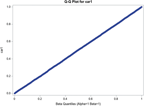
Figures 1a and 1b describes the distribution of annual mileage for car 1, combined for simplicity of exposition across study group. The results are similar within study group (data not shown). Figure 1a is reported as histograms, and the similar heights of these histograms imply that the results have a relatively similar likelihood of falling within the bins (0 to 2,500), (2,501 to 5,000), … , (47,501 to 50,000). This is a characteristic of the uniform distribution bounded by 0 and 50,000, denoted by U(0;50,000). Figure 1b is a Q-Q plot, a method which statisticians use to assess how closely data follows a specified distribution. Here, it plots observed quantiles against the quantiles which would be expected were the distribution U(0;50,000). The data almost perfectly follow a 45-degree line, indicating that the observed and expected quantiles were nearly coincident, and thus that the observed data in fact very closely follow this distribution. Results for cars 2–4 are similar (data not shown). In practice, encountering data which follows a distribution precisely rather than approximately can be a red flag that those data might have been simulated.

Figure 1a. Histogram of car 1 annual mileage.

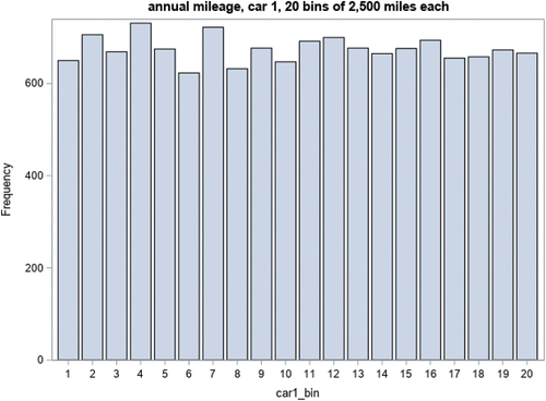
Figure 1b. QQ plot for car 1 annual mileage.

To comment, were this an actual misconduct review our statistical recommendation would be that the annual mileage data are substantively implausible, consistent with being simulated from a uniform distribution, and thus are very likely to be fabricated. What follows is an attempt to discover how this putative fabrication took place. Such an exploration is a necessary part of a murder mystery, and a significant portion of the work by DC but, we emphasize, not a necessary part of a forensic statistical analysis. In other words, the forensic statistical analysis could end with strong evidence for fabrication, recognizing that in many cases determining how this putative fabrication took place is not realistically possible. For simplicity of exposition, we will replace “putative fabrication” with “fabrication,” recognizing that, in an actual misconduct review, conclusions about fabrication are not the responsibility of the statistician.

Mechanistic questions

For simplicity, some questions about the mechanism of the fabrication can be stated in terms of car 1. Stipulating that the annual mileage D-C is fabricated, which variables were altered: C, D or both? How was the signal quantifying the impact of the honesty statement A added? It turns out that some clues include end digits and fonts.

Annual mileage: End digit preference

A mileage of 896 has a first digit of 8 and an end digit of 6. In this context, end digit preference refers to the tendency for humans to report annual mileage in round numbers ending in 0, 00, and 000. End digit preference has been used in previous forensic analyses (Al-Marzouki et al. 2005; Diekmann 2007; Mosimann, Wiseman, and Edelman 1995; Mosimann et al. 2002; Pickett 2020; Pitt and Hill 2013), and is based on “Benford’s law,” which essentially states that the distribution of the rightmost digit of many naturally occurring phenomena ought to be approximately uniform (Benford 1938). This property should also hold for simulated data, and so can be used to distinguish between data reported by humans and data generated by simulation.

Table 3 summarizes the end digit preference for the car 1 mileage at times 1 and 2. In the absence of end digit preference, all the entries should be 10% (apart from sampling variation). This is observed at time 2 but not time 1. Moreover, at time 1 the preferred end digit is 0, as would be expected, with the other end digits having similar rates of preference. This suggests that the data from time 2 are simulated, whereas some or all of the data from time 1 are real.

Table 3. End digit preferences, car 1.

End digit	Time 1	Time 2
0	23.9%	10.4%
1	8.1%	10.1%
2	8.5%	9.9%
3	8.6%	10.0%
4	8.4%	9.8%
5	9.2%	10.1%
6	8.5%	9.8%
7	8.4%	9.8%
8	8.1%	9.8%
9	8.3%	10.1%

The same phenomenon also occurs for the tendency to round by 10s and 100s, as illustrated in Table 4. For example, annual mileage which is rounded to the nearest 100 is over 100 times more likely at time 1 than at time 2.

Table 4. End digit preference for 0 (1 digit), 00 (2 digits), and 000 (3 digits), car 1.

Source	1 digit	2 digits	3 digits
Time 1	23.9%	14.5%	10.3%
Time 2	10.4%	1.1%	0.1%
Expected if no end digit preference	10.0%	1.0%	0.1%

Results for cars 2–4 are substantially similar (data not shown).

Possible mechanisms of fabrication

In the spirit of Lieutenant Columbo’s mastery of minutiae, DC notes that exactly half of the observations are in Cambria font and the other half are in Calibri font. More precisely, this pattern only applies to the time 1 data for car 1. All of the other data fields for cars 1–4 are in Calibri font. Presumably, the fabrication involved copying within Excel. Moreover, the copying occurred by selecting a record based on time 1 data for car 1 and then using the entire data record, with the font of the index field (but not the others) somehow being altered during the copying and pasting. Lieutenant Columbo would have performed extensive experiments on how copying and pasting works within Excel, the perpetrator would have proposed alternative explanations, which would then be demonstrated to be impossible.

Table 5 illustrates that the time 1 data in Calibri font exhibited strong end digit preference whereas the time 1 data in Cambria font did not. This suggests that the time 1 observations in the half of the dataset in Calibri font are real, whereas the time 1 observations in the half of the dataset in Cambria font are simulated.

Table 5. End digit preference for 0 (1 digit), 00 (2 digits), and 000 (3 digits), car 1, time 1.

Source	Calibri	Cambria	Expected
Per 1000	20.64%	0.07%	0.10%
Per 100	27.94%	1.17%	1.00%
Per 10	37.89%	9.99%	10.00%

DC noted that there are pairs of records (i.e., one member in Calibri font, the other in Cambria) having similar mileage at time 1. Moreover, they hypothesized that a random number was added to the record in the Cambria font, likely drawn from a U(0;1,000) distribution, in order to make the duplication less obvious. Although establishing motive requires induction, one possible explanation for the copying is to double the sample size and thus increase the credibility of the results. Another possible explanation is that the sample size is correct, and the perpetrators simply chose to execute the fabrication by modifying half the dataset.

Because of the large number of overlapping records, it is impossible to definitely match a Cambria record to its twin (except, perhaps, in the extremes of the distribution). As a simple check of the above hypothesis, the time 1 records for car 1 with Cambria fonts were placed in ascending order, the same was done for the corresponding records with Calibri font, the files were merged, and a difference score was calculated. The intention is to roughly, although not precisely, replicate the putative matching. All difference scores were positive, and fell between 0 and 1,000. The difference scores had a mean of 501, approximately the mean of a U(0,1000) distribution, although the shape did not correspond to that distribution, which is consistent with our matching algorithm being less than perfect. Determining how to match pairs of records to most closely correspond to the use of a U(0,1000) distribution is a non-trivial statistical problem, which we considered to be out of the scope of the present analysis.

In summary, and in the spirit of separating fact from interpretation, we observed that:

• Time 1 data shows end digit preference for Calibri font but not Cambria.

• There are exactly the same number of observations in Calibri fort as in Cambria.

• After approximately pairing observations with similar mileage, the time 1 mileage in Cambria font always exceeds the pair in Calibri font, by 0-1,000 miles.

• For each car, the annual mileage data range from 0 -50,000 miles.

• For each car, annual mileage equals time 2 mileage minus time 1 mileage.

Our interpretation of the above is that:

• Half of the time 1 data are real (i.e., the portion with Calibri font), with the other half copied and modified by the addition of a U(0;1,000) random variable.

• The annual mileage data are simulated from a U(0;50,000) distribution.

• The annual mileage data were simulated first, then the time 2 odometer reading was adjusted so that time 2 minus time 1 equals annual mileage.

This still leaves the question of how the signal was added, which was not definitively answered by DC. The first two rows of Table 6 summarize the annual mileage for car 1 in the actual dataset. The third row illustrates the results obtained from simulating 6,700 data values from a U(0;50,000) distribution. The results are quite similar, except that the means in the first two rows of the table are shifted by approximately 1,250 miles in either direction. The similarities in the standard deviations, minima, maxima, and shape (data not shown) support the hypothesis that the annual mileages are in fact based on a U(0;50,000) distribution and then modified as described.

Table 6. Observed and simulated data for car 1, time 1.

	N	Mean	S.D.	Minimum	Maximum
Observed: Sign Bottom	6,664	23,623	14,506	15	49,982
Observed: Sign Top	6,824	26,205	14,226	8	49,997
Simulated: U(0,50000)	6,700	25,095	14,343	12	49,998
Simulated: Sign Bottom with adjustment at 2,500 miles	6,700	23,906	14,303	12	49,998
Simulated: Sign Top with adjustment at 47,500 miles	6,700	26,282	14,287	18	49,998

The mechanism for adding the signal must satisfy the constraint that the pattern of the standard deviations, minima and maxima aren’t substantially changed, nor is the shape of the distribution. For example, subtracting 1,250 miles from each observation in the “Form Top” won’t work – although the shape and standard deviation are unchanged, the minimum would become negative and the maximum won’t exceed 48,750. Overcoming this constraint is a significant challenge, which Lieutenant Columbo would have overcome by visualizing in detail the various ways that the murder in question could have been committed. In that spirit, the Lieutenant would have assumed that the proposed mechanism of fabrication could be implemented using simple manipulations within Excel, especially since the information from the fonts suggests that copying and pasting involving half the dataset was taking place. The rationale for preferring simple manipulations is that the perpetrator wasn’t anticipating being audited, and so took the path of least resistance.

The bottom two rows of the spreadsheet illustrate how the signal might have been added. Considering the annual mileage for the “Sign Bottom” group:

• Create a U(0;50,000) random variable, with a mean of 25,000

• For half the records, perhaps the half with Cambria font, subtract 2,500 from U for all records to obtain U*. The mean of U* will be 22,500.

• Notice that U* is negative with U < 2,500 and so set U* = U for those records. The impact on the mean is trivial, and so the mean for the overall population is approximately the average of 25,000 and 22,500 – namely 23,750.

The actual mechanics could have been accomplished by sorting an Excel spreadsheet by A and D, highlighting those records with A = “Sign Bottom” and D > 2500, and then using a using a global function to subtract 2,500 from the highlighted records. The “Sign Top” group would follow the same procedure but replacing subtraction with addition, and the mean for the overall population is approximately 26,250.

Mileage from the other cars could have been generated similarly. Indeed, it is possible that the dataset was originally structured in a long-thin format, with one record per car per responder, in which case separate operations wouldn’t be required for each car but could instead be performed in a single step.

Table 7 applies this procedure, and calculates average annual mileage per policyholder (i.e., as reported by Shu et al.). As a general result from standard distributional theory, the more cars per policyholder, the more the shape of the distribution of average annual mileage moves away from the uniform and eventually toward the normal, thus explaining why overall annual mileage, which is the average of up to four cars, isn’t uniformly distributed. The observed and simulated data are substantially similar, and thus a plausible mechanism for the putative fabrication has been demonstrated. As another fictional detective once observed: “once you eliminate the impossible, whatever remains, however improbable, must be the truth” (https://sherlockholmesquotes.com).

Table 7. Observed and simulated annual mileage data by car.

	Study group	N	Mean	S.D.	Minimum	maximum
Observed	Sign Bottom	6,664	23,671	12,621	24	49,982
Simulated	Sign Bottom	6,664	23,916	12,413	25	49,997
Observed	Sign Top	6,824	26,098	12,253	31	49,997
Simulated	Sign Top	6,824	26,223	12,402	12	49,992

Additional clues about motive: The spreadsheet

Returning to the Excel spreadsheet provided by the investigators, it is actually organized in an unusual fashion. What the insurer would typically have delivered to the investigators are columns A–J – that is, the raw data only. The investigators would have:

• Definitely derived the primary outcome, M.

• Probably derived intermediate variables to aid in the calculation of M.

The primary outcome variable was included in the spreadsheet provided by the investigators to DC, presumably as an aid to users. This is consistent with usual practice.

What seems unusual is the intermediate variables that are included in the spreadsheet (i.e., K and L). Here, it is important to recognize that, from an analytical perspective, annual mileages by car are far more natural than average mileage per policyholder. The reason is that average mileage per policyholder at times 1 and 2 has no other analytical use than as intermediate variables in the formula for creating M. On the other hand, creating new variables containing annual mileage by car is analytically useful, as these are the outcomes for the car-specific analyses which would be performed as a matter of course.

In other words: the investigators would appear to have no particular reason to create K and L, but would have a good statistical reason to create annual mileage by car. Instead of including the intermediate variables K–L in their spreadsheet, they could instead have:

• Included no intermediate variables – or –

• Included annual mileage by car as intermediate variables, as per usual statistical practice

We hypothesize that the reason that K and L are included in the spreadsheet might have been to direct the user’s attention away from the primary mechanism by which the data were fabricated, which involved annual mileage by car. Including another set of intermediate variables might distract the user from creating annual miles by car, and instead induce them to limit their focus to the average annual mileage per policyholder, which isn’t as problematic (although still less than pristine, having 50,000 as an upper bound) and also doesn’t provide direct information about the mechanism by which the fabrication took place.

Recognizing that motive always involves induction, these additional clues might (or might not) provide information about motive, to be ultimately judged by the misconduct reviewers. This is the sort of detail about which Lieutenant Columbo would have commented “it might not mean anything, but I need to clarify this for my report”

Statistical report

The statistician’s report would, ideally, be a combination of technical information (e.g., tables and figures) and a generally accessible narrative summary. The present communication, minus references to fictional detectives, illustrates one way that such a report might be organized. Although it might not always be realistic to do so, good statistical practice would suggest archiving the raw data and the computer code used to generate the information in the report, thus allowing the forensic analysis to be audited and verified. The Supplemental Materials contain this archive.

Discussion

Research misconduct is defined as “falsification, fabrication and plagiarism, and does not include honest error or differences of opinion” (https://grants.nih.gov/policy/research_integrity/definitions.htm). Questionable research practices, such as performing multiple analyses and then preferentially reporting those which support one’s hypotheses, fall somewhere in between innocently inappropriate and malign (Troy, Samsa, and Rockhold 2021). Lack of reproducibility – for example, an inability to reproduce the steps in performing a study, managing its data, and analyzing its data – can be a contributory factor to misconduct, but can also follow from the combination of good intentions and common but less than pristine practices around data provenance.

Each of the above problems is best addressed before the fact rather than afterward. Some preventive approaches include the development of standard operating procedures around data management, development and proactive documentation of statistical analysis plans, changes in promotion criteria to deemphasize gratuitous publication, and changes in organizational culture which encourage concerned individuals to speak up without penalty. If successful, such changes will reduce but not eliminate the need for post hoc investigation. Sometimes, performing misconduct investigations is a statutory requirement, as is the case for allegations of misconduct in federally funded research. Sometimes, these investigations are associated with management of financial conflict of interest, which provides an additional motive for misbehavior. Sometimes, these investigations are simply motivated by the importance of institutional integrity.

Research misconduct investigations can include forensic statistical analysis. Our case study illustrates how such a forensic statistical analysis is performed (see also (Dahlberg and Davidian 2010)). Stipulating the data were fabricated as hypothesized here, and without speculating as to who is ultimately responsible for the fabrication, with the simple addition of a dead body this could be a lost episode of Columbo – fabrication within a study of honesty, a crucial clue provided by a suspicious font, etc. One can easily envision Columbo asking the perpetrator “one more thing: about these fonts … ,” and that individual preferring confession and a lifetime of incarceration to enduring additional questioning on the topic. Although end digit preference is often used to identify data values that have likely been fabricated by humans, it is unusual for it to be used to contrast legitimate human-generated responses from simulated responses within the same study.

Our hope is that this communication has helped to illustrate what forensic statistics can – and cannot – realistically accomplish. We believe that it is helpful for those who interact with forensic statisticians to recognize that statisticians define their task as (1) ascertaining whether the original raw database is correct; (2) ascertaining whether the raw database has been correctly transformed into a statistical analysis file; and (3) determining whether the statistical analyses are appropriate. Forensic statisticians can assist their colleagues by, among others (1) keeping these three tasks separate; (2) distinguishing fact from opinion so as to avoid gratuitous advocacy; and (3) minimizing unnecessary detail to support clarity. Here, the key and straightforward observation is that car mileage cannot realistically follow a uniform distribution – everything else is only relevant to producing a comprehensive “police report.”

Quite often, the issue in question pertains to the accuracy of the “original” raw data. This was true for the Potti case (Baggerly and Coombes 2009, 2010, 2011), where the initial reviewers apparently assumed that a publicly available file provided to them purporting to be the raw data from which a genomic signature was derived was pristine, whereas in fact its labels were inaccurate (among other problems). Because of poor documentation of the data management and analyses used to create the genomic signature, 1,500 person-hours of effort from biostatisticians at M.D. Anderson Cancer Center were ultimately required to plausibly recreate what was done, and their recommendations for the information required to support clinical “omics” publications – in other words, what it takes to get the documentation right for similar studies – included: ”(1) the raw data; (2) the code used to derive the results from the raw data; (3) evidence of the provenance of the raw data so that labels could be checked; (4) written descriptions of any non-scriptable analysis steps; and (5) prespecified analysis plans, if any” (Baggerly and Coombes 2011). These biostatisticians reported that their efforts originally started with being asked the question of whether the genomic signature developed by Potti and colleagues should be used in patient care at their institution, as part of their due diligence they reviewed the relevant publications, became concerned that the signature in question might be inaccurate, at which point ethical imperatives predominated.

Quite obviously, the bloggers from DC invested a significant amount of time in their work as well. We do not speculate why.

Were this an actual forensic statistical analysis our recommendation would be that that demonstrating that annual mileage follows a uniform distribution provides sufficient evidence about fabrication, and thus that identifying the precise mechanism by which the fabrication occurred need not be a requirement. Indeed, it many circumstances discovery of mechanism won’t be possible. In our case study, a plausible mechanism was only discovered because (1) extraordinarily detailed scrutiny by the bloggers contributing to DC (e.g., noticing that a database contained two fonts which aren’t dramatically different in appearance); and (2) the choice of an implausible distribution on the part of the fabricator – presumably out of convenience combined with the assumption that the results wouldn’t ever be audited. Our efforts extend the analysis in DC by identifying a possible mechanism by which the signal (i.e., the difference in annual mileage between the two study groups) might have been added to the database. Although in this case life happened to imitate art, requiring that it do so is not a realistic expectation.

Archive dataset

The Supplemental Materials contain an Excel file, a SAS dataset and an annotated SAS program.

Disclosure statement

No potential conflict of interest was reported by the author(s).

Supplementary material

Supplemental data for this article can be accessed online at https://doi.org/10.1080/08989621.2024.2329265

Additional information

Funding

The author(s) reported there is no funding associated with the work featured in this article.

References

- Al-Marzouki, S. S., S. Evans, T. Marshall, and I. Roberts. 2005. “Are These Data Real? Statistical Methods for the Detection of Data Fabrication in Clinical Trials.” BMJ: British Medical Journal 331 (7511): 267–270. https://doi.org/10.1136/bmj.331.7511.267.
- Baggerly, K. A., and K. R. Coombes. 2009. “Deriving Chemosensitivity from Cell Lines: Forensic Bioinformatics and Reproducible Research in High-Throughput Biology.” The Annals of Applied Statistics 3 (4): 1309–1334. https://doi.org/10.1214/09-AOAS291.
- Baggerly, K. A., and K. R. Coombes. 2010. “Retraction Based on Data Given to Duke Last November, but Apparently Disregarded.” Cancer Letter 36 (39): 4–6.
- Baggerly, K. A., and K. R. Coombes. 2011. “What information should be required to support clinical “omics” publications?” Clinical Chemistry 57 (5): 688–690. https://doi.org/10.1373/clinchem.2010.158618.
- Benford, F. 1938. “The Law of Anomalous Numbers.” In Proceedings of the American Philosophical Society, 78 (4): 551–572. http://www.jstor.org/stable/984802.
- Dahlberg, J. E., and N. M. Davidian. 2010. “Scientific Forensics: How the Office of Research Integrity Can Assist Institutional Investigations of Research Misconduct During Oversight Review.” Science and Engineering Ethics 16 (4): 713–765. https://doi.org/10.1007/s11948-010-9208-4.
- Diekmann, A. 2007. “Not the First Digit! Using Benford’s Law to Detect Fraudulent Scientific Data.” Journal of Applied Statistics 34 (3): 321–329. https://doi.org/10.1080/02664760601004940.
- Mosimann, J., J. Dahlberg, N. Davidian, and J. Krueger. 2002. “Terminal Digits and the Examination of Questioned Data.” Accountability in Research 9 (2): 75–92. https://doi.org/10.1080/08989620212969.
- Mosimann, J. E., C. V. Wiseman, and R. E. Edelman. 1995. “Data fabrication: can people generate random digits?” Accountability in Research 4 (1): 31–55. https://doi.org/10.1080/08989629508573866.
- Pickett, J. T. 2020. “The Stewart Retractions: A Quantitative and Qualitative Analysis.” Econ Journal Watch 17 (1): 152–190.
- Pitt, J. H., H. Z. Hill Statistical detection of potentially fabricated numerical data: a case study. 2013. Available from https://www.semanticscholar.org/paper/Statistical-Detectin-pf-Potentially-Fabriacted-A-Pitt-Hill/95e5805e45bae47e050b9f430bbd7e41b3045688.
- Shu, L. L., N. Mazar, F. Gino, D. Ariely, and M. H. Bazerman. 2012. “Signing at the Beginning Makes Ethics Salient and Decreases Dishonest Self-Reports in Comparison to Signing at the End.” Proceedings of the National Academy of Science 109 (38): 15197–15200. https://www.pnas.org/cgi/doi/10.1073/pnas1209746109.
- Troy, J., G. Samsa, and F. Rockhold. 2021. “Institutional Approaches to Preventing Questionable Research Practices. Accountability in Research: Policies and Quality Assurance.” Accountability in Research 30 (4): 252–259. https://doi.org/10.1080/08989621.2021.1986017.