Comparison of multivariate models and variable selection algorithms for rapid analysis of the chemical composition of field crops

ABSTRACT

This study evaluates the use of visible and near-infrared spectroscopy for rapid prediction of total carbon, total nitrogen, and total phosphorus concentrations in field crop samples. Two multivariate models (partial least squares regression and support vector machine regression) were compared. In addition, four spectral variable selection algorithms (competitive adaptive reweighted sampling, genetic algorithm, uninformative variable elimination, and variable importance for projection) were applied with support vector machine regression to determine the most accurate predictions. The results showed that support vector machine regression performed better than partial least squares regression for predicting the three chemical compositions. The combination of competitive adaptive reweighted sampling and support vector machine regression outperformed the other models for the predictions of total carbon and total nitrogen with high coefficients of determination of 0.91 and 0.90, respectively. For the determination of total phosphorus, the prediction accuracy of competitive adaptive reweighted sampling was comparable with the best result obtained from genetic algorithm with the coefficients of determination of 0.73 and 0.77, respectively. In conclusion, the support vector machine regression combined with competitive adaptive reweighted sampling has great potential to accurately determine the chemical composition of field crops using the visible and near-infrared spectroscopy.

KEYWORDS:

• Model calibration
• support vector machine regression
• total carbon
• total nitrogen
• total phosphorus
• visible and near-infrared spectroscopy

Introduction

The elements carbon (C), nitrogen (N), and phosphorus (P) are essential chemical compositions of plants and play vital roles in function maintenance and adaptation to environmental stresses (Elvidge 1990; Gillon et al. 1999). Rapid, reliable, and nondestructive measurements using visible and near-infrared reflectance spectroscopy (Vis–NIR) to predict plant biochemistry are fundamental for understanding the biogeochemical cycling of plants in agroecosystems and are thus widely used to manage crop nutrient status, recommend fertiliser applications, and provide crop parameters for process simulations (Elvidge 1990; Foley et al. 1998; van Maarschalkerweerd and Husted 2015; Chodak 2008). Over the past few decades, Vis–NIR has been used extensively to predict a wide variety of important chemical constituents and nutritional properties (e.g. crude protein, fibres, lignin, cellulose, and minerals) in field crops (e.g. Clark et al. 1987; Elvidge 1990; Foley et al. 1998; Gillon et al. 1999; Cozzolino et al. 2006; Chodak 2008; Huang et al. 2009; van Maarschalkerweerd and Husted 2015; Hetta et al. 2017). Varying degrees of success in predicting total carbon (Ct), total nitrogen (Nt), and total phosphorus (Pt) contents in plant materials have been reported in the literature (e.g. Vázquez de Aldana et al. 1995; García-Ciudad et al. 1999; Gillon et al. 1999; Petisco et al. 2005; Karimi et al. 2008; Parsons et al. 2011). However, previous studies that have used Vis–NIR for chemical determinations of field crops have typically been restricted to a limited range of species, such as a single species or just a few species (e.g. Vázquez de Aldana et al. 1995; Gillon et al. 1999; Cozzolino et al. 2006; Huang et al. 2009; Parsons et al. 2011; Hetta et al. 2017), and often limited numbers of samples (e.g. García-Ciudad et al. 1999; Petisco et al. 2005; Parsons et al. 2011). This may lead to unstable calibrations and inconsistent prediction results.

Partial least squares regression (PLSR) is one of the most commonly used multivariate techniques (Vasques et al. 2008; Viscarra Rossel and Behrens 2010; Vohland et al. 2011). However, the complex non-linear relationships between independent and dependent variables suggests that the use of linear models, such as PLSR, may be insufficient (Thomas and Haaland 1990; Viscarra Rossel and Behrens 2010). Compared to linear methods, non-linear techniques, such as support vector machine regression (SVMR), have been effectively applied in non-linear modelling applications and have generally exhibited higher performance results (Vohland et al. 2011). The SVMR method has several desirable characteristics, including good generalisation abilities, robustness of the regression function, and the ability to address sparse data (Rao and Gopalakrishna 2009). SVMR improves the prediction accuracy of biochemical constituents of plants (Chauchard et al. 2004; Li et al. 2007; Karimi et al. 2008; Xu et al. 2016). However, most of the published results have been based on full-spectrum wavebands (400–2500 nm).

A calibration process based on full-spectrum wavebands is too time-consuming and inconvenient to fulfil the high-speed features of spectroscopic techniques. Nonetheless, high redundancy, collinearity and, sometimes, noise in full Vis–NIR spectral data may decrease the estimation capability and computing efficiency of the SVMR model (Abrahamsson et al. 2003; Andersen and Bro 2010). Therefore, pre-selecting an optimum set of spectral variables instead of using the full-spectrum wavebands, is essential to improve the performance of the SVMR model and/or reduce model complexity (Shi et al. 2014). A number of variable selection approaches have already been developed, such as competitive adaptive reweighted sampling (CARS), genetic algorithm (GA), random frog, successive projections algorithm (SPA), uninformative variable elimination (UVE), and variable importance for projection (VIP) (Leardi et al. 1992; Centner et al. 1996; Abrahamsson et al. 2003;Chong and Jun 2005; Zou et al. 2010; Li et al. 2014). These studies have shown that more accurate calibration models can be achieved by selecting the most informative spectral variables instead of using the full-spectrum wavebands (Leardi and González 1998; Shi et al. 2014; Vohland et al. 2014; Wang et al. 2014). However, none of these proposed variable selection techniques have achieved universal acceptance, because a variable selection that works well for one application may be inappropriate for another. Therefore, the optimisation of SVMR models, coupled with an appropriate variable selection, is expected to establish a better calibration model for the practical use of Vis–NIR spectroscopy.

This study was conducted using a wide variety of crop samples from seven species across China. The main objectives were: (1) to compare the performance of PLSR and SVMR for the rapid predictions of Ct, Nt, and Pt in field crops; (2) to evaluate the benefit of four variable selection methods (CARS, GA, UVE, and VIP) with SVMR models to improve estimation of the selected chemical compositions; and (3) to identify the information content of the statistically selected spectral variables.

Materials and methods

Crop sampling and chemical analysis

The study was performed in the principal agricultural areas of China. Representative crop samples were collected from 60 counties or cities from most provinces across China to guarantee a heterogeneous sample set that represented a wide range of locations, species, cultivars, soil characteristics, growing climates, and farm management strategies. A total of 312 crop samples from seven species were collected from 2011 to 2013 at full maturity, including 141 rice (Oryza sativa L.), 78 maize (Zea mays L.), 51 wheat (Triticum aestivum L.), 24 oilseed rape (Brassica napus L.), 9 soybean [Glycine max (L.) Merr.], 6 cotton (Gossypium hirsutum L.), and 3 hulless barley (Hordeum vulgare L.) samples. Each fresh crop sample consisted of several individuals from three locations in one field. In the present study, shoots (including leaves, branches, and stems) and roots were manually separated in the field, not including grains or seeds. In total, 624 individual subsamples were collected and separately subjected to chemical analyses and Vis–NIR scanning.

All plant samples were chopped into <2 cm lengths, dried at 65°C in a forced-air oven to constant weight (approximately 48 h), and then ground using a cyclone mill (DFT-50, Wenling LINDA Machinery Co., Ltd., Wenling, China) until they passed through a 1-mm sieve. The prepared samples were stored in airtight Ziploc bags in a dark room prior to chemical analyses and Vis–NIR scanning. Reference constituent concentrations (i.e. Ct, Nt, and Pt) of plant samples were analyzed using the standard wet chemical methods after H₂SO₄–H₂O₂ digestion in the laboratory (Lu 2000). Total C was measured using the potassium dichromate method, and Nt was determined by the semimicro automated Kjeldahl method. Total P was measured using the molybdenum-blue colorimetric method. All chemical analyses were performed in duplicate and expressed on a dry weight basis (g kg⁻¹).

Spectral measurements

Before Vis–NIR scanning, all milled plant subsamples were oven-dried at 50°C for 2 h. After cooling, reflectance spectra of the samples were acquired in a black room using an ASD FieldSpec 3 portable spectroradiometer (Analytical Spectral Devices, Boulder, USA) with a spectral range of 350 nm to 2500 nm and a spectral resampling interval of 1 nm. Each plant sample was placed in an aluminum tray (1.5-cm depth and 9.5-cm inner diameter), and the surface was gently pressed with a spatula before levelling. Plant samples were illuminated using four 50-W quartz-halogen lamps, which were mounted on tripods at 30 cm to collect light beams that were 45° from vertical using an 8° field-of-view sensor that was perpendicular to the sample at a distance of 25 cm. To ensure that variation within a sample was detected, ten reflectance spectra were measured in four directions by successively rotating the sample by 90° between readings. The forty readings were averaged to generate a representative spectral signature for each plant sample. A white Spectralon panel (Labsphere, North Sutton, NH, USA) was used to obtain the reflectance factor, which is the sample reading divided by the reference panel reading and multiplied by the absolute reflectance of the reference panel.

Spectral pretreatments

Reflectance data were exported from binary to ASCII file format using ViewSpec Pro software (Analytical Spectral Devices, Boulder, USA). The reflectance was then transformed to absorbance using the expression A = log(1/R), where A is absorbance and R is reflectance. For the entire spectrum, the output resolution of the spectral data was 1 nm. To eliminate the noise at the edges of each spectrum, the raw spectra were reduced to between 380 nm and 2450 nm. They were then resampled in 5 nm increments across this range because of the highly collinear spectra, which resulted in 415 bands for subsequent analyses. No general recommendation can be given whether the data set should be pre-processed or which method would be best suited. Therefore, several mathematical preprocessing steps were applied to the crop spectra using the PLS Toolbox version 8.0 (Eigenvector Research, Inc., Wenatchee, WA, USA) run under MATLAB version R2012b (The MathWorks, Inc., Natick, MA, USA). These pretreatments included: (1) the first and second derivatives to reduce baseline variation and enhance spectral features; (2) Savitzky–Golay smoothing with a 10-band window, which reduces baseline variation and enhances spectral features; (3) a standard normal variate transform (SNV) to reduce the spectral variability (light scattering); (4) a standard multiplicative scatter correction (MSC), which removes additive and/or multiplicative signal effects; (5) detrending; and (6) a combination of the previous pretreatments. Finally, the spectral data were mean centred. Each pretreatment was then calibrated to Ct, Nt, and Pt concentrations with a multivariate model. The best spectral pretreatment was selected for each crop composition based on the lowest root mean squared error of cross-validation (RMSE_CV) in the calibration data sets. Only the combination of Savitzky–Golay smoothing with first derivatives and SNV transformation was determined and used in all subsequent modelling (data not shown).

Variable selection methods

Different spectral variable selection algorithms were used to select predictor variables, which were calibrated via the SVMR models for crop constituent concentrations. The targeted algorithms included CARS, GA, UVE, and VIP. The CARS, UVE, and VIP procedures were implemented in the libPLS package version 1.95 (Li et al. 2014). The GA procedure was carried out in the PLS Toolbox. A brief summary of each of these techniques is provided below, and key references are cited for more detailed information.

CARS is an effective wavelength selection algorithm based on the principle of ‘survival of the fittest’ (Li et al. 2009). First, it removes the wavelengths that have small regression coefficients by an exponentially decreasing function (EDF). Then, the ratio of the wavelengths is calculated by an EDF equation. The steps of each sampling run can be described as follows: (a) model sampling using the Monte Carlo (MC) principle; (b) wavelength selection based on EDF; (c) competitive wavelength selection using adaptive reweighted sampling; and (d) evaluation of the subset using cross-validation (Li et al. 2009). Finally, wavelengths that have little or no effective information are eliminated, while the subset with the lowest root mean squared error of cross-validation (RMSE_CV) is retained as effective wavelengths (Vohland et al. 2014). The optimal number of MC sampling runs was set to 100.

The GA method is based on evolutionary biology (Leardi et al. 1992). It is a kind of global optimisation searching method inspired by Darwin’s theory of natural selection (Leardi and González 1998). Through the operation of genetic processes such as reproduction, mutation, and selection, along with continuous genetic iteration, the variable with a better fit for the fitness function is selected (Leardi et al. 1992). Algorithmically, the basic GA steps can be outlined as follows: (a) coding of the variable; (b) initiation of the population; (c) evolution of the response; (d) reproduction; (e) mutation; and (f) repetition of the process until a stopping criterion is reached (Malhotra et al. 2011). Generally, the stopping criterion includes a maximum number of generations, a maximum target outcome value for the fitness or a set number of generations (Leardi and González 1998). Evaluation is performed by means of the fitness function which depends on the specific problem and is the optimisation objective of the GA. Since GA does not carry out the fitness evaluation of the population, PLSR was used for its fitness function in this study. The cross-validated RMSE_CV from PLSR was used as a fitness value for evaluating the population. The optimal band combinations are selected when the RMSE_CV is minimal. In this study, the parameter values of the GA for each crop constituent were set based on the preliminary tests (Table 1).

Table 1. The key parameters of genetic algorithm (GA) for the prediction of different crop constituents.

Constituents	Ct	Nt	Pt
Population size	64	64	64
Window width	1	1	1
Penalty slope	0.05	0.05	0.03
Mutation rate	0.005	0.01	0.005
Crossover	double	double	double
Max generations	100	100	100
Replicate runs	10	10	10
LVs	14	13	14
RMSECV (g kg^−1)	16.74	1.75	0.43

Note: Ct, total carbon; Nt, total nitrogen; Pt, total phosphorus; LVs, the optimal number of latent variables; RMSE_CV, root mean squared error of cross-validation.

UVE is a novel variable selection algorithm based on stability analysis of the PLSR regression coefficients (Centner et al. 1996). In the UVE algorithm, a PLSR regression coefficient matrix is calculated through a leave-one-out validation. Then, the reliability of each variable can be quantitatively measured according to its stability. The stability of variable $j$ can be calculated through the following equation (Centner et al. 1996):(1) $s_j=\frac{\mathrm{mean}\left(b_j\right)}{\mathrm{std}\left(b_j\right)},j=1,2,\cdots ,p$(1) where $\mathrm{mean}\left(b_j\right)$ and $\mathrm{std}\left(b_j\right)$ are the mean and standard deviation, respectively, of the regression coefficients of variable $j$. The larger the absolute stability, the more important the corresponding variables. A variable with a stability between the cutoff thresholds is regarded as uninformative and is eliminated. In this study, the cutoff value used was 99% of the $\left|s_j^{\mathrm{random}}\right|$ (Zou et al. 2010). UVE can eliminate the uninformative variables for modelling noise and can thus enhance the impact of validation on modelling and increase the probability of selecting the best model.

The VIP method estimates the importance of each variable based on the weight of the loading factors from each component (Viscarra Rossel and Behrens 2010). The VIP scores can be calculated using the following equation (Wold et al. 2001):(2) $VI{P}_k\left(a\right)=K\sum _a{w}_{ak}^2\left(\frac{SS{Y}_a}{SS{Y}_t}\right)$(2) where $VI{P}_k\left(a\right)$ is the importance of the $k_{th}$ predictor variable based on a model with a factors, $w_{ak}$ is the corresponding loading weight of the $k_{th}$ variable in the $a_{th}$ PLSR factor, $SS{Y}_a$ is the explained sum of squares of the response variable by a PLSR model with a factors, $SS{Y}_t$ is the total sum of squares of the response variable, and $K$ is the total number of predictor variables. A variable with a VIP score close to or above 1.0 is then considered important for the model and is thus selected for further use (Chong and Jun 2005; Andersen and Bro 2010).

Data analysis

We compared two multivariate methods to derive Vis–NIR models of the three crop constituents: PLSR and SVMR. As the frequency distributions of Ct, Nt, and Pt were skewed, a natural logarithm transformation was applied to each crop constituent to normalise the data for the model development using PLSR. Estimated crop constituents (calibration and validation) from PLSR models were back-transformed to original units (g kg⁻¹) to assess model quality. The SVMR methods are nonparametric and do not assume an approximate Gaussian distribution of the target variable; therefore, we used Ct, Nt, and Pt in their original units to derive SVMR models.

Because PLSR is a classical calibration method and can always provide relatively acceptable results, the performance of the FS-PLSR model was used as a reference to evaluate other models developed with selected spectral variables. Leave-one-out cross-validation with as many as 20 factors was used to determine the optimum number of PLS components (or latent variables) required to calibrate each model and calculate the predicted values of a calibration subset to assess the robustness of each model (Wold et al. 2001). The residuals of cross-validation predictions were pooled to calculate the RMSE_CV. For a PLSR model of each crop constituent, the optimum number of components was attained when the addition of a supplementary component led to an increase of less than 6% in the explained variance (Peltre et al. 2011). Additionally, outliers related to the Vis–NIR data should be detected and removed during cross-validation (Vasques et al. 2008). Spectral samples with a strong influence (leverage) on the model (leverage >5 times the average leverage of all samples) were removed as calibration outliers, and cross-validation was repeated (Peltre et al. 2011). The resulting linear PLSR models were of the equation:(3) $y={\beta }_0+{\beta }_{\lambda 1}{A}_{\lambda 1}+\cdots +{\beta }_{\lambda i}{A}_{\lambda i}$(3) Where $y$ is the predicted chemical composition, ${\beta }_0$ is the intercept, and ${\beta }_{\lambda i}$ is the regression coefficient for the transformed absorbance $A_{\lambda i}$ at wavelength $\lambda i$.

SVMR represents a relatively new non-linear model based on the statistical learning theory (Vapnik 1995; Smola and Schölkopf 2004). Using SVMR, a model hyperplane is derived that describes the empirical data as correctly as possible and minimises the distances from the hyperplane to the training data (Vapnik 1995). ε-SVM-regression (ε-SVMR) uses training data to obtain a model that is represented as an ε-insensitive loss function (tube, band) that maps independent data, with a maximum ε deviation from the dependent training data (Vohland et al. 2011). Error within the predetermined distance ε from the true value is ignored, and error greater than ε is penalised by parameter C. In the present study, a Gaussian radial basis function (RBF) was applied to determine the width of the kernel, and the parameters C and γ of the RBF were searched for with a systematic grid search method. The regularisation parameter γ determines the trade-off between the fitting error minimisation and the smoothness of the estimated function, which is used to improve the generalisation performance of the SVMR model (Thissen et al. 2004). These two parameters were optimised with γ values in the range of 2⁻¹–2¹⁰ and C values in the range of 2–2¹⁵, with adequate increments. For each combination of γ and C parameters, the optimal model parameters that minimise RMSE were determined by leave-one-out cross-validation. The SVMR model can be expressed as:(4) $y\left(\chi \right)=\sum _{i=1}^n{\alpha }_{i}K(\chi ,{\chi }_i)+b$(4) where $K(\chi ,{\chi }_i)$ is the kernel function, ${\chi }_i$ is the input vector, ${\alpha }_i$ is Lagrange multipliers called support value, and $b$ is the bias term.

The PLSR and SVMR calibrations were carried out in the PLS Toolbox. The optimal wavelengths selected by CARS, GA, UVE, and VIP were applied as inputs to establish new optimised SVMR models (i.e. CARS-SVMR, GA-SVMR, UVE-SVMR, and VIP-SVMR). The best predictive and robust model was then chosen by comparing the results of these models to the FS-PLSR and FS-SVMR models. For all calibration models, seventy percent of samples (n = 437) were selected for calibration using the Kennard-Stone algorithm for calibration, and the remaining samples (n = 187) were used for external validation (Kennard and Stone 1969). The Kennard-Stone algorithm selects two samples that are the furthest from each other in Mahalanobis distance and assigns them to the calibration and validation sets. The process continues sequentially until the desired number of calibration or validation samples is selected, yielding a uniform distribution of the data for spectroscopic modelling.

Model evaluation

The measured values vs. the values predicted from the calibration (cross-validation) or the independent validation data sets were compared using a simple regression. The coefficient of determination (R²) and RMSE were calculated to compare the accuracy of the different calibration models using the following equations (Williams 1987):(5) $R^2=\frac{{\sum }_{i=1}^n{\left({\hat{y}}_i-{\overline{y}}_i\right)}^2}{{\left(y_i-{\overline{y}}_i\right)}^2}$(5) (6) $\mathrm{RMSE}=\sqrt{\frac{{\sum }_{i=1}^n{\left({\hat{y}}_i-y_i\right)}^2}{n}}$(6) where $\hat{y}$ is the predicted value, $y$ is the measured value, $\overline{y}$ is the mean of measured values, $N$ is the number of data points. Generally, large values of R² and small RMSE values indicated a model with good predictive ability (Williams 1987). The results for R² and RMSE from the cross-validation and independent validation are labelled with the subscripts of CV and P, respectively. Statistical analyses were conducted with the SPSS statistical software package version 18.0 for Windows (SPSS Inc., Chicago, IL, USA). All of the procedures were tested on the Microsoft Windows 7 operating system with an Intel i7-2600 CPU and 8 GB RAM.

Results and discussion

Crop sample properties

Summary statistics for the calibration and validation data sets for the three constituents (i.e. Ct, Nt, and Pt) measured in the laboratory are provided in Table 2. A total of 16, 13, and 15 samples were eliminated from further analysis as spectral outliers from the calibration models for the Ct, Nt, and Pt predictions, respectively. Overall, Ct ranged from 201.80 g kg⁻¹ to 461.54 g kg⁻¹, Nt from 2.41 g kg⁻¹ to 21.58 g kg⁻¹, and Pt from 0.29 g kg⁻¹ to 4.23 g kg⁻¹. The averaged values of Ct, Nt, and Pt were 372.10, 8.60 and 1.08 g kg⁻¹ for the calibration set and 366.85, 8.03 and 1.07 g kg⁻¹ for the validation set, respectively. The majority of crop samples had large Ct values and small Nt and Pt values, which resulted in large skewness in their concentration distributions (Table 2). After the logarithm transformation, the distributions of Ct, Nt, and Pt in the calibration set closed to normal with a skewness of −0.70, −0.15, and 0.04, respectively. The concentration ranges of the three constituents in the calibration set covered the validation set, which ensured a reasonable estimate of the model.

Table 2. Descriptive statistics for the concentrations of total carbon (Ct), total nitrogen (Nt), and total phosphorus (Pt) (expressed on a dry matter basis, g kg⁻¹) of field crops in China for the calibration and validation subsets.

Constituents	nSample	nOut	Range	Mean	CV	Skewness	Kurtosis
Calibration
Ct	437	16	201.80–461.54	372.10	9.80	−1.85	5.98
Nt	437	13	2.41–21.58	8.60	37.63	0.81	0.56
Pt	437	15	0.29–4.23	1.08	55.29	1.45	3.28
logCt	437	16	5.31–6.13	5.91	1.89	−0.70	0.89
logNt	437	13	0.88–3.07	2.08	18.15	−0.15	−0.17
logPt	437	15	−1.24–1.44	−0.06	−160.11	0.04	−0.52
Validation
Ct	187	–	207.18–423.83	366.85	9.66	−2.07	6.47
Nt	187	–	3.10–18.75	8.03	31.53	0.83	1.37
Pt	187	–	0.30–3.63	1.07	51.37	1.41	3.29
logCt	187	–	5.33–6.04	5.90	1.88	−0.80	0.69
logNt	187	–	1.13–2.93	2.04	15.54	−0.22	0.30
logPt	187	–	−1.20–1.29	−0.04	−179.15	0.11	−0.53

Note: logCt, logNt, and logPt mean natural log-transformed Ct, Nt, and Pt, respectively; n_Sample, number of samples used for calibration or validation; n_Out, number of outliers discarded during calibration; CV, coefficient of variation (%).

Spectral characterisation

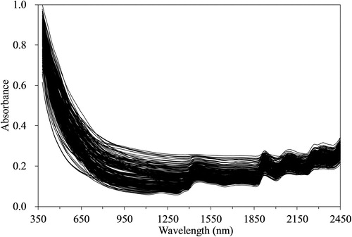
The absorbance spectra in the 380–2450 nm range obtained from crop samples are shown in Figure 1. Although there was some variation among samples, especially in the level of each curve, all absorbance spectra had generally the same shape. The spectral range from 380 to 1100 nm presented little interpretable absorption bands, and lower signal-to-noise ratio. For the NIR region of the spectrum, some prominent absorbance peaks and troughs tended to occur at the same wavelengths across all crop samples. Several peaks were observed at wavelengths of 1400 nm, 1900 nm, 2100 nm, and 2330 nm. The first two peaks correspond to water absorption, whereas lignin and cellulose bands generally range from 2100 to 2300 nm. No obvious differences were observed, indicating that the crop samples from different species can be considered as the same category for model development.

Figure 1. Visible and near-infrared absorbance spectra of crop samples for total carbon prediction (n = 608).

Predictions of crop constituents from optimised SVMR models

To obtain the optimal model with a robust predictive ability and a small number of input variables, four variable selection methods (i.e. CARS, GA, UVE, and VIP) were conducted to determine the most effective wavelength variables, which reflected the spectral characteristics to predict the crop constituents. The CARS algorithm was first introduced to minimise the dimensionality of Vis–NIR spectra and select the effective variables (wavelengths). The 74, 34, and 67 effective variables were selected by CARS for the prediction of Ct, Nt, and Pt, respectively (Table 3). In GA, the same spectral calibration data and the corresponding concentrations of crop constituents were entered as input for the GA-based wavelength selection. The RMSE_CV reached the lowest values of 16.74 g kg⁻¹, 1.75 g kg⁻¹, and 0.43 g kg⁻¹ when 76, 82, and 70 variables were selected by GA with 14, 13, and 14 latent variables for Ct, Nt, and Pt, respectively (Table 1). For the UVE method, the spectral variables (n = 134, 165, and 147) were regarded as informative variables and were then used for the SVMR calibrations for Ct, Nt, and Pt, respectively (Table 3). When using the VIP method, there were 51.6%, 23.9%, and 32.8% variables with VIP score ≥1.0; these were classified as informative for predicting Ct, Nt, and Pt, respectively.

Table 3. Statistical evaluation of different variable selection methods used to predict the crop constituents (expressed on a dry matter basis, g kg⁻¹) derived by PLSR and SVMR models for the calibration and validation subsets using visible and near-infrared (Vis–NIR) reflectance spectroscopy.

Model	Calibration				Validation
	nSample	Time	$R_{CV}^2$	RMSECV	$R_P^2$	RMSEP
Ct
FS-PLSR	415	–	0.86	13.48	0.84	14.02
FS-SVMR	415	–	0.90	11.58	0.87	13.39
CARS-SVMR	74	0.12	0.94	9.21	0.91	11.29
GA-SVMR	76	47.00	0.93	10.09	0.88	12.71
UVE-SVMR	134	0.68	0.91	10.75	0.87	13.02
VIP-SVMR	214	0.10	0.93	9.63	0.90	11.36
Nt
FS-PLSR	415	–	0.85	1.27	0.81	1.49
FS-SVMR	415	–	0.90	1.03	0.86	0.95
CARS-SVMR	34	0.12	0.92	0.94	0.90	0.83
GA-SVMR	82	47.50	0.89	1.06	0.86	0.97
UVE-SVMR	165	0.68	0.91	0.97	0.88	0.90
VIP-SVMR	99	0.10	0.91	0.95	0.87	0.92
Pt
FS-PLSR	415	–	0.65	0.35	0.58	0.46
FS-SVMR	415	–	0.72	0.33	0.70	0.31
CARS-SVMR	67	0.12	0.76	0.31	0.73	0.29
GA-SVMR	70	48.75	0.80	0.28	0.77	0.27
UVE-SVMR	147	0.68	0.80	0.27	0.76	0.28
VIP-SVMR	136	0.10	0.77	0.29	0.74	0.30

Note: Ct, total carbon; Nt, total nitrogen; Pt, total phosphorus; FS, full spectrum; PLSR, partial least squares regression; SVMR, support vector machine regression; CARS, competitive adaptive reweighted sampling; GA, genetic algorithm; UVE, uninformative variable elimination; VIP, variable importance for projection; n_Sample, number of spectral variables used in the model calibration; Time, computation time (minutes) required by variable selection algorithms; R², coefficient of determination; RMSE, root mean squared error (g kg⁻¹). The results for R² and RMSE from the cross-validation and independent validation are labelled with the subscripts of CV and P, respectively.

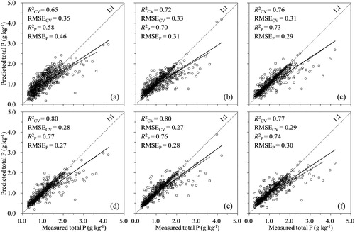
Spectroscopic data were calibrated and validated against the measured crop constituents (i.e. Ct, Nt, and Pt) using the CARS-SVMR, GA-SVMR, UVE-SVMR, and VIP-SVMR models. The scatterplots of the predicted vs. measured crop constituents for the different models are illustrated in Figures 2–4, and the descriptive regression statistics are provided in Table 3. The estimated crop constituent contents were all positively correlated with the measured values. The FS-SVMR and four optimised SVMR models (Ct: $R_{CV}^2$ = 0.90–0.94, RMSE_CV = 9.21–11.58; Nt: $R_{CV}^2$ = 0.90–0.92, RMSE_CV = 0.94–1.06; Pt: $R_{CV}^2$ = 0.72–0.80, RMSE_CV = 0.27–0.33) provided better prediction accuracies than the FS-PLSR models (Ct: $R_{CV}^2$ = 0.86, RMSE_CV = 13.48; Nt: $R_{CV}^2$ = 0.85, RMSE_CV = 1.27; Pt: $R_{CV}^2$ = 0.65, RMSE_CV = 0.35) based on the calibration sets. Better predictions were also achieved by the SVMR models using the independent validation sets compared with the FS-PLSR models (Table 3), suggesting that the SVMR models improved the prediction accuracies of all studied crop constituents. In terms of the variable selection methods studied, the four optimised SVMR models obtained different prediction accuracies for the crop constituents compared to the FS-SVMR models. The most accurate determination of Ct ($R_P^2$ = 0.91; RMSE_P= 11.29) was achieved by CARS-SVMR in independent validation (Table 3). Similarly, the best result was obtained with CARS-SVMR for Nt ($R_P^2$ = 0.90; RMSE_P= 0.83). However, the prediction of Pt ($R_P^2$ = 0.77; RMSE_P= 0.27) was best achieved with GA-SVMR, which was lower than that obtained for Ct and Nt predictions. Notably, the accuracy of the VIP-SVMR model ($R_P^2$ = 0.90; RMSE_P= 11.36) was similar to that of the CARS-SVMR model for the determination of Ct, whereas the accuracy of the UVE-SVMR model ($R_P^2$ = 0.76; RMSE_P= 0.28) for Pt prediction was similar to that of the GA-SVMR model. Compared to the FS-PLSR models, the CARS-SVMR models for Ct and Nt and the GA-SVMR models for Pt reduced their RMSE_P values by 19.5%, 44.3%, and 41.3%, respectively. For the determination of Ct, the UVE-SVMR models did not improve the prediction accuracy compared with FS-SVMR, whereas for Nt, the GA-SVMR models did not improve the prediction accuracy compared with FS-SVMR. Successful determinations of Ct and Nt by Vis–NIR are clearly explained by the absorption of infrared radiation by the O-H, C-H, and N-H bonds present in the plants, whereas the measurements of Pt appeared to be limited, as P is not spectrally active in the Vis–NIR range (De Boever et al. 1994; Gillon et al. 1999). Among the optimised SVMR models for Pt, CARS-SVMR yielded the lowest accuracy ($R_P^2$ = 0.73; RMSE_P= 0.29), though it was still comparable with GA-SVMR. As shown in Figure 2, the PLSR and SVMR models for Ct both exhibited a greater deviation from the 1:1 lines at lower concentrations. In contrast, these models for Pt produced a greater deviation from the 1:1 lines at higher concentrations (Figure 4).

Figure 2. Scatter plots of the measured and Vis–NIR predicted total C from different calibration models: (a) FS-PLSR, (b) FS-SVMR, (c) CARS-SVMR, (d) GA-SVMR, (e) UVE-SVMR, and (f) VIP-SVMR. Predictions on the calibration set during cross-validation (black circles, black regression lines) and predictions on the independent validation set (blue squares, blue regression lines). The 1:1 line (dotted) is shown in each figure.

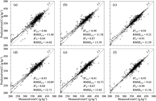
Figure 3 . Scatter plots of the measured and Vis–NIR predicted total N from different calibration models: (a) FS-PLSR, (b) FS-SVMR, (c) CARS-SVMR, (d) GA-SVMR, (e) UVE-SVMR, and (f) VIP-SVMR. Predictions on the calibration set during cross-validation (black circles, black regression lines) and predictions on the independent validation set (blue squares, blue regression lines). The 1:1 line (dotted) is shown in each figure.

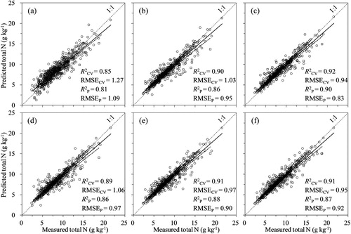
Figure 4. Scatter plots of the measured and Vis–NIR predicted total P from different calibration models: (a) FS-PLSR, (b) FS-SVMR, (c) CARS-SVMR, (d) GA-SVMR, (e) UVE-SVMR, and (f) VIP-SVMR. Predictions on the calibration set during cross-validation (black circles, black regression lines) and predictions on the independent validation set (blue squares, blue regression lines). The 1:1 line (dotted) is shown in each figure.

Many other studies have also shown SVMR models to perform better than other multivariate methods. For example, Chauchard et al. (2004) reported that SVMR (R² = 0.86) was superior to PLSR (R² = 0.77) for predicting total acidity in fresh grapes based on a validation data set of 185 samples. Li et al. (2007) compared SVMR and PLSR methods for the prediction of the protein N-glycosylation and reported that higher accuracy was found with the SVMR method. In a recent study, SVMR and PLSR methods were compared by Xu et al. (2016), who also found SVMR ($R_P^2$ = 0.88; RMSE_P= 4.28) modelling to be superior to PLSR ($R_P^2$ = 0.82; RMSE_P= 5.22) for the determination of rice root density using 73 validation samples. The results obtained in this study are in agreement with the above results. Collinearity in Vis–NIR data can lead to problems if the estimation methods depend on the order in which the input variables are presented. However, in the case of projection methods like SVMR, where the input data are first projected onto a higher dimensional space before they are employed in the estimation process, such methods are not affected by collinearity (Morlini 2006). Therefore, it can be concluded that SVM modelling is a better approach to predictive machine learning-based modelling, especially for Vis–NIR analysis.

Although the FS-SVMR models yielded better results for predicting Ct, Nt, and Pt than FS-PLSR, the input spectral data had 415 variables, including informative and uninformative variables with regard to the crop constituents. The interference of uninformative variables would not only decrease the prediction precision but also complicate the SVMR models. Utilisation of variable selection in processed spectra is a very important step to solve such problems (Zou et al. 2010). Due to the variable selection, a new reduced spectral matrix was generated by selecting the Vis–NIR spectra only at the important variables that contained the most relevant spectral information of the crop constituents. The new matrix was then used to replace the full-range spectra to build new SVMR models to determine the crop constituents. Among the variable selection methods studied, CARS selected the fewest spectral variables for the determination of Ct, Nt, and Pt, where the percentages of the spectral variables used to develop the CARS-SVMR models were 17.8%, 8.2%, and 16.1%, respectively (Table 3). Apparently, more spectral variables were considered important by UVE and VIP than by CARS and GA. For Ct and Nt predictions, the number of spectral variables selected by VIP was approximately three times greater than that of the CARS method. The CARS-SVMR and GA-SVMR models, with a few wavelengths, both worked especially well for the calibration and validation sets. In contrast, UVE selected many wavelengths (≥ 134) that might have high correlations between the adjacent wavelengths. These redundant variables might inevitably weaken the performance of the UVE-SVMR models. Therefore, the overall results indicated that CARS was a powerful way to select effective wavelengths for spectroscopic analyses. Moreover, the results demonstrated that Vis–NIR spectroscopy combined with CARS-SVMR or GA-SVMR was an efficient alternative to rapidly and noninvasively determine the crop constituents.

Comparison of the CARS, GA, UVE, and VIP methods

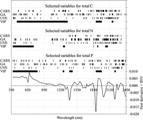
The specific wavelengths of the effective variables selected by CARS, GA, UVE, and VIP for the prediction of Ct, Nt, and Pt are shown in Figure 5. In general, the CARS, GA, and UVE techniques produced sparser distributions of effective variables in the full-spectrum wavebands than VIP. The variables selected by CARS for Nt were primarily concentrated on the NIR region. Obviously, some successive wavelength ranges were chosen by VIP for each crop constituent. For instance, three wavelength ranges (455–1380 nm, 1900–2005 nm, and 2190–2215 nm) for Ct prediction and four wavelength ranges (380–760 nm, 1300–1330 nm, 1925–1940 nm, and 2070–2110 nm) and one wavelength at 1855 nm for Nt prediction were identified by VIP (Figure 5). Several spectral variables were all selected by CARS, GA, and UVE for predicting Ct (1730 nm, 1925 nm, 2150 nm, 2155 nm, 2195 nm, 2200 nm, and 2305 nm), Nt (1930 nm, 2060 nm, 2105 nm, 2260 nm, 2285 nm, and 2360 nm), and Pt (670 nm, 1800 nm, 1835 nm, 2260 nm, 2280 nm, 2325 nm, and 2375 nm). These effective variables selected by the four methods are generally in line with those of other studies on the prediction of C, N, and P (Elvidge 1990; García-Ciudad et al. 1999; Ruano-Ramos et al. 1999; Petisco et al. 2005; Chodak 2008), although some differences (i.e. ±20 nm) were observed at specific wavelength absorptions.

Figure 5. The comparison of spectral variables (indicated by the black vertical lines) selected by CARS, GA, UVE, and VIP from the Vis–NIR spectra transformed by the combination of the first derivative and SNV.

Compared to the UVE and VIP methods, CARS selected the smallest number of effective variables (n ≤ 74) as input data matrices in a shorter computing time (0.12 min) and obtained the highest prediction accuracy for predicting Ct and Nt (Table 3). For Pt prediction, GA selected a smaller number of effective variables (n = 70) as input data matrices in the longest computing time (48.75 min) and achieved the highest prediction accuracy. Reducing large spectral data sets to parsimonious representations is valuable for more efficient storage, computation and transmission. The training time could be greatly reduced by the SVMR model because it increased with the square of the number of training samples and linearly with the number of variables (Chauchard et al. 2004). In addition, with fewer variables, it is possible to use a simpler and cheaper spectrophotometer. Thus, the effective wavelengths obtained by CARS could be used to develop inexpensive in situ Vis–NIR instruments (or sensors) for the rapid and nondestructive determination of the crop constituents.

As a popular heuristic optimisation technique, GA obtained better results for predicting Pt. However, GA is complex and it is time-consuming to find the exact global optimum (Leardi and González 1998). It took more than 47 min to extract 70–82 effective variables for the predictions of crop constituents, whereas CARS took only 0.12 min in the same computing platform. Furthermore, GA presents a tremendous configuration challenge to the user because of the numerous adjustable factors (e.g. fitness function, convergence criteria, mutation rate, crossover, initial population, and generations; see Table 1) that affect the selection outcomes (Zou et al. 2010; Wang et al. 2014). The GA method is stochastic, the results are realisation dependent, and variable selections may not be reproducible (Andersen and Bro 2010; Shi et al. 2014). Therefore, the judicious selection of these parameters is critical. The speed and configuration problems limit the circumstances under which some applications may be successfully applied, and they require a considerable level of expertise on the part of the user (Zou et al. 2010; Malhotra et al. 2011). Nevertheless, the applications of UVE did not lead to satisfactory results with more variables (Table 3), perhaps because UVE tended to select instable variables that had a small signal-to-noise ratio and thus affected the model prediction accuracy (Zou et al. 2010). Similarly, the VIP method did not improve the prediction statistics for Nt and Pt. It only gave satisfactory results for Ct prediction but with the largest number of spectral variables. One possible reason is that VIP focuses on the weighting of variables in the projection but ignores the stability of variables (Liao et al. 2012). Moreover, some variables whose stability was the same as the noise played an important role within the latent projection but showed poor performance in the SVMR models.

In our study, considering the estimation accuracy, the number of selected variables, and the computation time, it could be concluded that the CARS method was the most suitable variable selection approach in this study. Variable selection is necessary, and better predictions can be obtained using a few chemically meaningful effective wavelengths, not a continuous band or a combination of several continuous bands, because the high collinear wavelengths may reduce the stability of the calibration model. Many previous studies have shown that better predictions could be obtained by CARS when compared to GA, UVE, and VIP (e.g. Li et al. 2009; Vohland et al. 2014; Han et al. 2015). For example, Li et al. (2009) used the CARS and UVE approaches for variable selection in PLSR models. They found that CARS-PLSR achieved the lowest prediction error (RMSE_CV= 0.1067) for corn protein prediction compared to the FS-PLSR (RMSE_CV= 0.1500) and UVE-PLSR (RMSE_CV= 0.1214) models. For corn moisture data, the RMSE_CV values were 0.0006, 0.0032, and 0.0229 in the CARS-PLSR, UVE-PLSR, and FS-PLSR models, respectively. Vohland et al. (2014) successfully implemented the CARS approach in the soil data set, and they concluded that the approach was simple and accurate and involved reasonable and parsimonious variable selection. Han et al. (2015) reported that the CARS-PLSR (RMSE_P = 0.55–0.81) model was more reasonable than the UVE-PLSR (RMSE_P = 0.89–1.23) model for the determination of glycated hemoglobin content.

Implications for practice

Many studies have focused on estimating the biochemical contents of different plant species with Vis–NIR spectroscopy (e.g. Elvidge 1990; Petisco et al. 2005; Chodak 2008). For example, Chodak (2008) developed PLSR models for Ct, Nt, and Pt of diverse plant materials with an R² of 0.86–0.99, 0.94–0.98, and 0.94–0.95, respectively. Using PLSR and derivative transformations, Petisco et al. (2005) obtained best calibration R² statistics: 0.99 for Nt and 0.94 for Pt. Similarly to these studies, our study obtained comparable results for Ct and Nt with calibrated R² of 0.94 and 0.92, respectively. The small differences between calibration and validation statistics for Ct, Nt, and Pt indicate the robustness of the calibrations (Table 3). All these results confirmed the feasibility of estimating chemical composition of field crops with Vis–NIR spectroscopy. Application of Vis–NIR is worthwhile only when large sample numbers are to be analyzed. However, a model’s generalisation ability is affected by many factors such as sample representativeness, multivariate model selection, and model complexity. Although the proposed SVMR models provided good performance, some specific considerations, described below, must be kept in mind.

First, the plant samples used in our study were heterogeneous, covering a large range of locations, species, and cultivars. The calibration equations were valid only for the sample population for which they were built and cannot be used to predict compositions in samples from outside this population. Any new samples must first be included in the calibration set. A possible solution of this problem is building large and diverse spectral libraries using archived plant samples in the future. Moreover, a local calibration procedure is an alternative to be considered for improving both the accuracy and the robustness of predictive models. The local algorithm operates by selecting samples in large data sets containing spectra similar to the sample being analyzed. The selected samples are then used to develop a specific calibration equation for predicting the constituents of an unknown sample. Second, the performance of SVMR is dependent on the optimal combination of the regularisation parameter C and RBF kernel parameter γ. The strategy of selecting an adequate calibration set for parameterizations is of fundamental importance to ensure models with good generalisation ability, especially when such models are calibrated from heterogeneous samples. Third, overfitting may be caused when redundant and uncorrelated wavebands exist in the calibration process. In our study, the input of SVMR was replaced by the selected spectral features and the cross-validation technique was used, which both can greatly improve the generalisation performance.

Disclosure statement

No potential conflict of interest was reported by the authors.

Notes on contributors

Shengxiang Xu is an Associate Professor at the Institute of Soil Science, Chinese Academy of Sciences, Nanjing, People’s Republic of China. His current work is focused on soil carbon and nitrogen dynamics, remote sensing and information technology in resources and environment.

Meiyan Wang is an Assistant Professor at the Institute of Soil Science, Chinese Academy of Sciences, Nanjing, People’s Republic of China. Her current work is focused on evolution of soil resources and soil remediation technology.

Xuezheng Shi is a Senior Professor at the Institute of Soil Science, Chinese Academy of Sciences, Nanjing, People’s Republic of China. His research interest is focused on soil quality and sustainability, soil physical properties and soil management.

Additional information

Funding

This work was supported by grants from the National Key Research and Development Program of China [grant number 2017YFC0503906], the National Natural Science Foundation of China [grant number 41771253], the 135 Plan and Frontier Fields Program of the Institute of Soil Science [grant number ISSASIP1651], and the Strategic Priority Research Program of the Chinese Academy of Sciences [grant number XDA05050500].

References

- Abrahamsson C, Johansson J, Sparéna A, Lindgren F. 2003. Comparison of different variable selection methods conducted on NIR transmission measurements on intact tablets. Chemometr Intell Lab. 69:3–12. doi: 10.1016/S0169-7439(03)00064-9
- Andersen CM, Bro R. 2010. Variable selection in regression–a tutorial. J Chemometr. 24:728–737. doi: 10.1002/cem.1360
- Centner V, Massart DL, De Noord OE, De Jong S, Vandeginste BM, Sterna C. 1996. Elimination of uninformative variables for multivariate calibration. Anal Chem. 68:3851–3858. doi: 10.1021/ac960321m
- Chauchard F, Cogdill R, Roussel S, Roger JM, Bellon-Maurel V. 2004. Application of LS-SVM to non-linear phenomena in NIR spectroscopy: development of a robust and portable sensor for acidity prediction in grapes. Chemometr Intell Lab. 71:141–150. doi: 10.1016/j.chemolab.2004.01.003
- Chodak M. 2008. Application of near infrared spectroscopy for analysis of soils, litter and plant materials. Pol J Environ Stud. 17:631–642.
- Chong IG, Jun CH. 2005. Performance of some variable selection methods when multicollinearity is present. Chemometr Intell Lab. 78:103–112. doi: 10.1016/j.chemolab.2004.12.011
- Clark DH, Mayland HF, Lamb RC. 1987. Mineral analysis of forages by near infrared reflectance spectroscopy. Agron J. 79:485–490. doi: 10.2134/agronj1987.00021962007900030016x
- Cozzolino D, Fassio A, Fernández E, Restaino E, La Manna A. 2006. Measurement of chemical composition in wet whole maize silage by visible and near infrared reflectance spectroscopy. Anim Feed Sci Tech. 129:329–336. doi: 10.1016/j.anifeedsci.2006.01.025
- De Boever JL, Eeckhout W, Boucque CV. 1994. The possibilities of near infrared reflection spectroscopy to predict total-phosphorus, phytate-phosphorus and phytase activity in vegetable feedstuffs. NJAS-Wagen J Life Sc. 42:357–369.
- Elvidge CD. 1990. Visible and near infrared reflectance characteristics of dry plant materials. Int J Remote Sens. 11:1775–1795. doi: 10.1080/01431169008955129
- Foley WJ, McIlwee A, Lawler I, Aragones L, Woolnough AP, Berding N. 1998. Ecological applications of near infrared reflectance spectroscopy – a tool for rapid, cost-effective prediction of the composition of plant and animal tissues and aspects of animal performance. Oecologia. 116:293–305. doi: 10.1007/s004420050591
- García-Ciudad A, Ruano A, Becerro F, Zabalgogeazcoa I, Vázquez de Aldana BR, García-Criado B. 1999. Assessment of the potential of NIR spectroscopy for the estimation of nitrogen content in grasses from semiarid grasslands. Anim Feed Sci Tech. 77:91–98. doi: 10.1016/S0377-8401(98)00237-5
- Gillon D, Houssard C, Joffre R. 1999. Using near-infrared reflectance spectroscopy to predict carbon, nitrogen and phosphorus content in heterogeneous plant material. Oecologia. 118:173–182. doi: 10.1007/s004420050716
- Han Y, Chen JM, Pan T, Liu GS. 2015. Determination of glycated hemoglobin using near-infrared spectroscopy combined with equidistant combination partial least squares. Chemometr Intell Lab. 145:84–92. doi: 10.1016/j.chemolab.2015.04.015
- Hetta M, Mussadiq Z, Wallsten J, Halling M, Swensson C, Geladi P. 2017. Prediction of nutritive values, morphology and agronomic characteristics in forage maize using two applications of NIRS spectrometry. Acta Agr Scand B-S P. 67:326–333.
- Huang CJ, Han LJ, Yang ZL, Liu X. 2009. Exploring the use of near infrared reflectance spectroscopy to predict minerals in straw. Fuel. 88:163–168. doi: 10.1016/j.fuel.2008.07.031
- Karimi Y, Prashe S, Madani A, Kim S. 2008. Application of support vector machine technology for the estimation of crop biophysical parameters using aerial hyperspectral observations. Can Biosyst Eng. 50:13–20.
- Kennard RW, Stone LA. 1969. Computer aided design of experiments. Technometrics. 11:137–148. doi: 10.1080/00401706.1969.10490666
- Leardi R, Boggia R, Terrile M. 1992. Genetic algorithms as a strategy for feature selection. J Chemometr. 6:267–281. doi: 10.1002/cem.1180060506
- Leardi R, González AL. 1998. Genetic algorithms applied to feature selection in PLS regression: how and when to use them. Chemometr Intell Lab. 41:195–207. doi: 10.1016/S0169-7439(98)00051-3
- Li HD, Liang YZ, Xu QS, Cao DS. 2009. Key wavelengths screening using competitive adaptive reweighted sampling method for multivariate calibration. Anal Chim Acta. 648:77–84. doi: 10.1016/j.aca.2009.06.046
- Li HD, Xu QS, Liang YZ. 2014. Libpls: an integrated library for partial least squares regression and discriminant analysis. PeerJ PrePrints. 2:e190v191.
- Li SJ, Liu BS, Cai YD, Li YX. 2007. Predicting protein N-glycosylation by combining functional domain and secretion information. J Biomol Struct Dyn. 25:49–54. doi: 10.1080/07391102.2007.10507154
- Liao YT, Fan YX, Cheng F. 2012. On-line prediction of pH values in fresh pork using visible/near-infrared spectroscopy with wavelet de-noising and variable selection methods. J Food Eng. 109:668–675. doi: 10.1016/j.jfoodeng.2011.11.029
- Lu RK. 2000. Analytical methods of soil agricultural chemistry. Beijing: China Agricultural Science and Technology Press.
- Malhotra R, Singh N, Singh Y. 2011. Genetic algorithms: concepts, design for optimization of process controllers. Comput Inf Sci. 4:39–54.
- Morlini I. 2006. On multicollinearity and concurvity in some nonlinear multivariate models. Stat Method Appl. 15:3–26. doi: 10.1007/s10260-006-0005-9
- Parsons SA, Lawler IR, Congdon RA, Williams SE. 2011. Rainforest litter quality and chemical controls on leaf decomposition with near-infrared spectrometry. J Plant Nutr Soil Sc. 174:710–720. doi: 10.1002/jpln.201100093
- Peltre C, Thuriès L, Barthès B, Brunet D, Morvan T, Nicolardot B, Parnaudeau V, Houot S. 2011. Near infrared reflectance spectroscopy: a tool to characterize the composition of different types of exogenous organic matter and their behaviour in soil. Soil Biol Biochem. 43:197–205. doi: 10.1016/j.soilbio.2010.09.036
- Petisco C, García-Criado B, de Aldana BRV, Zabalgogeazcoa I, Mediavilla S, García-Ciudad A. 2005. Use of near-infrared reflectance spectroscopy in predicting nitrogen, phosphorus and calcium contents in heterogeneous woody plant species. Anal Bioanal Chem. 382:458–465. doi: 10.1007/s00216-004-3046-7
- Rao BV, Gopalakrishna SJ. 2009. Hardgrove grindability index prediction using support vector regression. Int J Miner Process. 91:55–59. doi: 10.1016/j.minpro.2008.12.003
- Ruano-Ramos A, García-Ciudad A, García-Criado B. 1999. Near infrared spectroscopy prediction of mineral content in botanical fractions from semi-arid grasslands. Anim Feed Sci Tech. 77:331–343. doi: 10.1016/S0377-8401(98)00245-4
- Shi TZ, Chen YY, Liu HZ, Wang JJ, Wu GF. 2014. Soil organic carbon content estimation with laboratory-based visible-near-infrared reflectance spectroscopy: feature selection. Appl Spectrosc. 68:831–837. doi: 10.1366/13-07294
- Smola AJ, Schölkopf B. 2004. A tutorial on support vector regression. Stat Comput. 14:199–222. doi: 10.1023/B:STCO.0000035301.49549.88
- Thissen U, Pepers M, Ustun B, Melssen WJ, Buydens LMC. 2004. Comparing support vector machines to PLS for spectral regression applications. Chemometr Intell Lab. 73:169–179. doi: 10.1016/j.chemolab.2004.01.002
- Thomas EV, Haaland DM. 1990. Comparison of multivariate calibration methods for quantitative spectral analysis. Anal Chem. 62:1091–1099. doi: 10.1021/ac00209a024
- van Maarschalkerweerd M, Husted S. 2015. Recent developments in fast spectroscopy for plant mineral analysis. Front Plant Sci. 6:169. doi: 10.3389/fpls.2015.00169
- Vapnik VV. 1995. The nature of statistical learning theory. New York: Springer-Verlag.
- Vasques GM, Grunwald S, Sickman JO. 2008. Comparison of multivariate methods for inferential modeling of soil carbon using visible/near-infrared spectra. Geoderma. 146:14–25. doi: 10.1016/j.geoderma.2008.04.007
- Vázquez de Aldana BR, García Criado B, García Ciudad A, Pérez Corona ME. 1995. Estimation of mineral content in natural grasslands by near infrared reflectance spectroscopy. Commun Soil Sci Plant. 26:1383–1396. doi: 10.1080/00103629509369379
- Viscarra Rossel RA, Behrens T. 2010. Using data mining to model and interpret soil diffuse reflectance spectra. Geoderma. 158:46–54. doi: 10.1016/j.geoderma.2009.12.025
- Vohland M, Besold J, Hill J, Fruend HC. 2011. Comparing different multivariate calibration methods for the determination of soil organic carbon pools with visible to near infrared spectroscopy. Geoderma. 166:198–205. doi: 10.1016/j.geoderma.2011.08.001
- Vohland M, Ludwig M, Thiele-Bruhn S, Ludwig B. 2014. Determination of soil properties with visible to near- and mid-infrared spectroscopy: effects of spectral variable selection. Geoderma. 223–225:88–96. doi: 10.1016/j.geoderma.2014.01.013
- Wang JJ, Cui LJ, Cao WX, Shi TZ, Chen YY, Cao Y. 2014. Prediction of low heavy metal concentrations in agricultural soils using visible and near-infrared reflectance spectroscopy. Geoderma. 216:1–9. doi: 10.1016/j.geoderma.2013.10.024
- Williams PC. 1987. Implementation of near-infrared technology. In: Williams P, Norris K, editor. Near-infrared technology. In the agricultural and food industries. 2nd ed. St. Paul, MN: American Association of Cereal Chemists; p. 145–169.
- Wold S, Sjöström M, Eriksson L. 2001. PLS-regression: a basic tool of chemometrics. Chemometr Intell Lab. 58:109–130. doi: 10.1016/S0169-7439(01)00155-1
- Xu SX, Shi XZ, Wang MY, Zhao YC. 2016. Determination of rice root density at the field level using visible and near-infrared reflectance spectroscopy. Geoderma. 267:174–184. doi: 10.1016/j.geoderma.2016.01.007
- Zou XB, Zhao JW, Povey MJW, Holmes M, Mao HP. 2010. Variables selection methods in near-infrared spectroscopy. Anal Chim Acta. 667:14–32. doi: 10.1016/j.aca.2010.03.048