Investigation of electromagnetic pulse scattering for metallic object classification using machine learning

ABSTRACT

This paper presents a metallic object classification method using various electromagnetic pulses. Each electromagnetic pulse irradiated eight metallic objects placed at increasing distances from 10 mm to 40 mm relative to the electromagnetic sensing system. The electromagnetic sensing system consisted of two RL circuits placed in close proximity. Objects were classified using linear (perceptron and multiclass logistic regression) and non-linear (neural network, 1D convolutional neural network (CNN) and 2D CNN) machine learning classifiers. The machine learning classifiers were trained on experimental data collected in an electromagnetically shielded laboratory. A 10-fold cross-validation mean classification accuracy of 99.4 ± 0.3% for the 1D CNN classifier, and 92.9 ± 1.2% for the 2D CNN classifier, was achieved using a rectangular chirp electromagnetic pulse. The rectangular chirp pulse outperformed two-sided decaying exponential, Gaussian, triangular, raised cosine, and rectangular pulses. All pulses had equal energy. While the rectangular chirp performed best overall, other pulses more accurately distinguished between some objects.

KEYWORDS:

• Convolutional neural network
• eddy currents
• electromagnetic pulse
• object classification
• machine learning

1. Introduction

Remote sensing of the environment provides many advantages, including acquiring information about an object without making physical contact. This is essential in the timely identification and classification of obscured metal objects. Some important applications of metallic object classification include detection of weapons [1], and automated sorting of objects in the recycling industry [2].

Electromagnetic pulses offer one such method of detecting metallic objects remotely in varying environments. The non-destructive nature of electromagnetic pulses makes it especially useful as the object may be recovered without being damaged. Prior research into the electromagnetic transient response of metals has primarily been conducted using non-destructive testing and evaluation methods known as pulsed eddy current testing. Researchers in the non-destructive testing and evaluation field have calculated plate thickness using a genetic programming algorithm [3], detected metal corrosion [4,5], and other metal defects using deep learning [6].

Electromagnetic waves at low frequencies tend to penetrate and propagate in non-perfect conductors, and are modulated according to conductivity, permittivity, permeability, size, shape, and defects. These variables create electromagnetic signatures that are unique to the metallic object, and therefore may be used for classification purposes. The electromagnetic signatures of metals are often processed, once recorded, to enhance the detection of features by algorithms. Some of these techniques include independent component analysis [7], principal component analysis [8], and convolutional neural networks [9].

Since the successful deep learning approach of AlexNet in 2012 [10], machine learning algorithms are able to more successfully detect objects [11]. There are multiple machine learning techniques in addition to CNNs, including kernel machines such as support vector machines, however CNNs have several advantages. Kernel machines do not automatically extract features, but CNNs do. Automated feature extraction makes CNNs more flexible as features do not need to be known in advance. Additionally, costs are reduced through automated feature extraction as human operators aren't needed. CNNs have the disadvantage of using a very large number of weights, making it difficult to obtain an understanding of the inner workings of the model. This of course also implies that CNNs require large computing resources for large data sets.

Despite inherent differences in electromagnetic output data, machine learning algorithms have been shown to be adaptable to a multitude of non-destructive testing problems. These include infrared thermography [12], ultrasound testing [13,14], and eddy current pulse testing [15]. Machine learning algorithms, including linear (perceptron, multiclass logistic regression) and non-linear (neural network, 1D CNN, 2D CNN) varieties, have been used to classify metallic objects using pulse induction electromagnetic data [16].

Deep learning methods have recently been applied to classification of high frequency electromagnetic signals [17], radar waveform recognition [18], and recognition of modulated radar signals [19]. A CNN with data augmentation using synthetic aperture radar was used for target detection [20]. Deep learning implemented on micro-Doppler signatures has been used for recognition of human activities including hand gesture recognition [21], and human activity recognition [22].

Many of these papers focus on high frequency signals that have extremely shallow penetration into metallic objects due to the skin effect. The focus of this paper is to extend the application of low frequency electromagnetic pulses for non-destructive testing to object classification. This work differs from previous research by focussing on low frequency electromagnetic signals that are capable of deeper penetration into metallic objects. Deeper penetration may potentially reveal information about the inner structure of an object that may improve classification accuracy.

This paper extends previous work by assessing the feasibility of using square integrable electromagnetic pulses for metallic object classification. Square integrable pulses have the advantage of a finite energy, and therefore may be directly compared. While each pulse may be generated with equal energy, individual pulses have unique signatures in the time and frequency domain. These unique signatures resulted in different metallic object classification accuracy.

The electromagnetic pulses used in the experiment include a two-sided decaying exponential, Gaussian, triangular, raised cosine, rectangular, and rectangular chirp. Time signature data, which is 1D, was classified using linear (perceptron and multiclass logistic regression) and non-linear (neural network and 1D CNN) machine learning algorithms. The time signature data was converted into a spectrogram and classified using a 2D CNN, which is a non-linear algorithm. The merit of using a 2D spectrogram instead of a time domain signal is the ability to use well-established computer vision techniques, such as CNNs, with automated feature extraction. The weights of the convolutional layers can be plotted to reveal the salient features used by the 2D CNN for object classification. The spectrogram also incorporates both frequency and time components into a single 2D structure.

The paper is organised as follows. Section 2 introduces the theory of the electromagnetic pulses, magnetically coupled circuits, and the energy of an electromagnetic pulse while Section 3 discusses the research method including the experiment, data set, and the structure of the CNN. Section 4 contains the experimental results and discussion and Section 5 concludes the work.

2. Theory

2.1. Two magnetically coupled RL circuits

A series RL circuit consists of a resistor and an inductor in series. Two series RL circuits in close proximity are magnetically coupled.

The transmitter RL circuit, referred to with subscript 1, has an external voltage $v_1\left(t\right)$ applied to induce a magnetic field in the inductor that via mutual inductance induces a change of current in the receiver RL circuit, referred to with subscript 2.

Using Kirchhoff's voltage law, for a voltage applied to the transmitter, the time domain equations describing the circuits are given by (1) $\begin{array}{rl}{v}_1\left(t\right)& =R_1{i}_1\left(t\right)+L_1\frac{\mathrm{d}{i}_1\left(t\right)}{\mathrm{d}t}-M\frac{\mathrm{d}{i}_2\left(t\right)}{\mathrm{d}t}\end{array}$(1) (2) $\begin{array}{rl}0& =R_2{i}_2\left(t\right)+L_2\frac{\mathrm{d}{i}_2\left(t\right)}{\mathrm{d}t}-M\frac{\mathrm{d}{i}_1\left(t\right)}{\mathrm{d}t},\end{array}$(2) where M is the mutual inductance and is given by (3) $M=\kappa \sqrt{L_1{L}_2},$(3) where κ is a coupling factor between zero and one. Rearranging for the time derivative of $i_2\left(t\right)$ of Equation (1(1) $\begin{array}{rl}{v}_1\left(t\right)& =R_1{i}_1\left(t\right)+L_1\frac{\mathrm{d}{i}_1\left(t\right)}{\mathrm{d}t}-M\frac{\mathrm{d}{i}_2\left(t\right)}{\mathrm{d}t}\end{array}$(1) ) and substituting into Equation (2(2) $\begin{array}{rl}0& =R_2{i}_2\left(t\right)+L_2\frac{\mathrm{d}{i}_2\left(t\right)}{\mathrm{d}t}-M\frac{\mathrm{d}{i}_1\left(t\right)}{\mathrm{d}t},\end{array}$(2) ) gives the state equations (4) $\begin{array}{rl}\frac{\mathrm{d}{i}_1\left(t\right)}{\mathrm{d}t}& =\frac{R_1{L}_2{i}_1\left(t\right)+R_{2}M{i}_2\left(t\right)-L_2{v}_1\left(t\right)}{M^2-L_1{L}_2}\end{array}$(4) (5) $\begin{array}{rl}\frac{\mathrm{d}{i}_2\left(t\right)}{\mathrm{d}t}& =\frac{M}{L_2}\frac{\mathrm{d}{i}_1\left(t\right)}{\mathrm{d}t}-\frac{R_2}{L_2}{i}_2\left(t\right).\end{array}$(5) These coupled first order differential equations may be solved using numerical methods such as the Runge-Kutta method.

2.2. Electromagnetic pulse

A time-dependent electromagnetic pulse $g\left(t\right)$ may be regarded as a superposition of waves of many frequencies [23]. The electrical system used to generate a pulse, such as a series RL circuit, has a transfer function that alters the electromagnetic pulse. The inverse Fourier transform of an electromagnetic pulse is given by (6) $g\left(t\right)=\frac{1}{\sqrt{2\pi }}{\int }_{-\mathrm{\infty }}^{\mathrm{\infty }}H\left(\omega \right)F\left(\omega \right){\mathrm{e}}^{\mathrm{j\omega t}}\mathrm{d}\omega ,$(6) where $H\left(\omega \right)$ is the transfer function of the system used to generate the pulse, and $F\left(\omega \right)$ is the input pulse. Use of Equation (6(6) $g\left(t\right)=\frac{1}{\sqrt{2\pi }}{\int }_{-\mathrm{\infty }}^{\mathrm{\infty }}H\left(\omega \right)F\left(\omega \right){\mathrm{e}}^{\mathrm{j\omega t}}\mathrm{d}\omega ,$(6) ) is justified as the system used to generate the pulse, and the pulse interaction with the metallic objects, respond linearly within the operating range of the experiments in this paper. The following section describes pulses used in the present work as shown in Figure 1.

Figure 1. Pulses used in this work in the time and frequency domain for (a) two-sided decaying exponential, (b) Gaussian, (c) triangular, (d) raised cosine, (e) rectangular and (f) rectangular chirp.

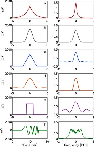
2.2.1. Two-sided decaying exponential pulse

The two-sided decaying exponential pulse subjects the objects to a second order increasing rate, i.e. a positive second derivative with respect to time. A two-sided decaying exponential pulse is given by (7) $f\left(t\right)=V_m{\mathrm{e}}^{-a|t|},$(7) where $V_m$ is the maximum voltage amplitude, $a=2\ln \left(2\right)/\tau$, and τ is the full width at half maximum.

The Fourier transform of the two-sided decaying exponential pulse is (8) $F\left(\omega \right)=\sqrt{\frac{2}{\pi }}\left(\frac{a{V}_m}{a^2+{\omega }^2}\right),$(8) which is a Lorentzian function.

2.2.2. Gaussian pulse

A Gaussian pulse has a Fourier transform that is also Gaussian. The Gaussian can also have a carrier frequency that centres the frequency distribution around a desired frequency. This property of Gaussian pulses may enable automated feature selection by finding frequencies that easily identify objects. The Gaussian pulse is given by (9) $f\left(t\right)=V_m{\mathrm{e}}^{-a{t}^2},$(9) where $V_m$ is the maximum voltage amplitude. The full width at half maximum τ may be controlled by setting (10) $a=\frac{4\ln 2}{{\tau }^2}.$(10) The Fourier transform of the Gaussian pulse is (11) $F\left(\omega \right)=\frac{V_m}{\sqrt{2a}}{\mathrm{e}}^{-{\omega }^2/4a}.$(11)

2.2.3. Triangular pulse

The triangular pulse is defined as (12) $f\left(t\right)=V_m\mathrm{tri}\left(2t/d\right)=\{\begin{array}{ll}{V}_m(1-|2t/d|),& |2t/d|<1\\ 0,& \mathrm{otherwise}\end{array},$(12) where $V_m$ is the maximum voltage amplitude, t is time, and d is the pulse width. The Fourier transform of the triangular pulse is (13) $F\left(\omega \right)=\frac{V_{m}d}{2\sqrt{2\pi }}{\mathrm{sinc}}^2\left(\frac{\mathrm{\omega d}}{4\pi }\right).$(13) The triangular function in the frequency domain is defined from $-\mathrm{\infty }<\omega <+\mathrm{\infty }$, however this is not realisable in practice. The triangular pulse has broad frequency components but unlike the rectangular pulse does not have a sudden voltage step response.

2.2.4. Raised cosine pulse

The raised cosine pulse is used in communications technology to minimise intersymbol interference by adjusting its roll-off factor. This pulse is included in the current work to investigate the feasibility of using multiple consecutive pulses with limited interference. The raised cosine pulse is given by [24] (14) $f\left(t\right)=\frac{V_m\cos \left(\mathrm{\pi \xi t}/\gamma \right)}{1-4{\xi }^2{t}^2/{\gamma }^2}\mathrm{sinc}\left(t/\gamma \right),$(14) where ξ is the roll-off factor, and $\gamma =1/\text{β}$ is the reciprocal of the symbol-rate β.

The Fourier transform of the raised cosine pulse is (15) $F\left(\omega \right)=\{\begin{array}{ll}{\displaystyle \frac{V_m\gamma }{\sqrt{2\pi }},}& |\omega |\le {\omega }_1\\ {\displaystyle \frac{V_m\gamma }{\sqrt{2\pi }}{[\sin \left(\frac{\gamma |\omega |-\pi (1+\xi )}{4\xi }\right)]}^2,}& {\omega }_1<|\omega |\le {\omega }_2\\ 0,& {\omega }_2<|\omega |\end{array},$(15) where ${\omega }_1=\pi (1-\xi )/\tau$ and ${\omega }_2=\pi (1+\xi )/\tau$.

2.2.5. Rectangular pulse

The rectangular pulse is defined as (16) $f\left(t\right)=V_m\mathrm{rect}\left(t/d\right)=\{\begin{array}{ll}0,& |t/d|>0.5\\ V_m,& |t/d|\le 0.5\end{array},$(16) where $V_m$ is the maximum voltage amplitude of the step, t is time, and d is the width of the pulse. The Fourier transform of the rectangular pulse is (17) $F\left(\omega \right)=\frac{V_{m}d}{\sqrt{2\pi }}\mathrm{sinc}\left(\frac{\mathrm{\omega d}}{2\pi }\right)$(17) The sinc function is defined from $-\mathrm{\infty }<\omega <+\mathrm{\infty }$, however this is not realisable in practice. There is a voltage rise time, and the perfect rectangular shape of the pulse cannot be achieved. The frequency distribution of the rectangular pulse provides a greater frequency range compared to other pulses. It also has a very sudden increase and decrease in voltage compared to other pulses and provides unique transient responses compared to other pulses.

2.2.6. Rectangular chirp pulse

A chirp is a signal in which the frequency increases or decreases with time. A linear up-chirp has a linearly increasing frequency with time and is given by (18) $f\left(t\right)=V_m\sin \left[2\pi (\frac{f_1-f_0}{2T}{t}^2+f_{0}t)\right],$(18) where $V_m$ is the maximum voltage amplitude of the chirp, $f_0$ is the starting frequency, $f_1$ is the final frequency, T is the time to sweep from $f_0$ to $f_1$, and t is the time. A chirp that ends with zero volts is desirable as a sudden jump to zero volts has a corresponding broadband frequency change. This broadband frequency change is reflected in a spectrogram of the signal and may negatively affect the classification accuracy of a CNN. To obtain a chirp that ends with zero phase, i.e. volts equal to zero at the end of the chirp, the end frequency may be chosen using the formula (19) $f_1=\frac{2K}{T}-f_0,$(19) where K is the number of oscillations.

A delayed chirp pulse is obtained by introducing a delay time $t_0$ and multiplying the chirp by a rectangular function. The chirp is delayed to ensure the spectrogram created from the signal captures all pulse data. The delayed chirp pulse is given by (20) $f(t-t_0)=\mathrm{rect}\left(\frac{t-t_d}{T}\right)V_m\sin \left[2\pi \left(\frac{f_1-f_0}{2T}\right(t-t_0{)}^2+f_0(t-t_0))\right],$(20) where $t_d=t_0+T/2$.

The Fourier transform of the chirp pulse is (21) $F\left(\omega \right)=\frac{V_m}{\sqrt{2\pi }}{\int }_{t_d-T/2}^{t_d+T/2}\sin \left[\frac{{\omega }_1-{\omega }_0}{2T}\right(t-t_0{)}^2+{\omega }_0(t-t_0)]{\mathrm{e}}^{-\mathrm{j\omega t}}\mathrm{d}t$(21)

2.3. Energy

The input energy in the driven circuit of an electromagnetic pulse in the time and frequency domain is [25] (22) $E={\int }_{-\mathrm{\infty }}^{+\mathrm{\infty }}v\left(t\right)i\left(t\right)\mathrm{d}t={\int }_0^{+\mathrm{\infty }}2|\overline{V}\left(f\right){|}^{2}G\left(f\right)\mathrm{d}f,$(22) where $v\left(t\right)$ is the voltage, $i\left(t\right)$ is the current, $v\left(t\right)i\left(t\right)$ is the power, $G\left(f\right)=\mathrm{Re}\left\{Y\right(f\left)\right\}$ is the real part of the admittance, $\overline{V}\left(f\right)$ is the Fourier transform of $v\left(t\right)$, $2|\overline{V}\left(f\right){|}^{2}G\left(f\right)$ is the energy spectral density, and the admittance of the transmitter circuit is (23) $Y\left(\omega \right)=\frac{R_2+\mathrm{j\omega }{L}_2}{R_1{R}_2+\mathrm{j\omega }(R_1{L}_2+R_2{L}_1)-L_1{L}_2(1-{\kappa }^2){\omega }^2}.$(23) The energy spectral density of all pulses with equal energy of 4.5 μJ is shown in Figure 2. Energy of 4.5 μJ was used in the current work for each pulse. This is the energy of a rectangular chirp pulse with parameters given in Table 1. All other pulses had their maximum voltage amplitude adjusted to obtain pulse energy equal to the rectangular chirp pulse energy due to ease of calculation and experimental setup. The width of the pulses ensures that the majority of the energy is contained below 1 kHz. This enables deep penetration into metallic objects and weak conductors such as seawater and the Earth, which is limited at high frequencies due to the skin effect.

Figure 2. Energy spectral density of the two-sided decaying exponential, Gaussian, triangular, raised cosine, rectangular and rectangular chirp pulse.

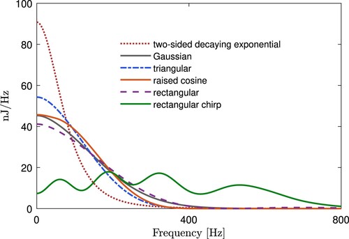
Table 1. Electromagnetic pulse parameters.

Pulse	Parameters
2SDE	$V_m=1.10$ V, $\tau =1.8$ ms
Gaussian	$V_m=1.06$ V, $\tau =2$ ms
Triangular	$V_m=1.12$ V, $d=4$ ms
Raised cosine	$V_m=1.13$ V, $\gamma =2$ ms, $\xi =0.8$
Rectangular	$V_m=1.01$ V, $d=2$ ms
Chirp	$V_m=1.00$ V, $T=10$ ms, $f_0=0$ Hz, $f_1=$800 Hz

2.4. Skin depth

The skin depth in a good conductor, such as steel and aluminium, is [26] (24) $\delta \left(f\right)\approx \sqrt{\frac{1}{\mathrm{\pi f}{\mu }_r{\mu }_0\sigma }},$(24) where f is the frequency of the electromagnetic wave, ${\mu }_r$ is the relative permeability of the conductor, ${\mu }_0$ is the vacuum permeability, and σ is the electrical conductivity of the conductor. The skin depths at different frequencies of D6ac steel [27] (${\mu }_r=77$, $\sigma =3.6$ MS/m) and aluminium [28] (${\mu }_r=1$, $\sigma =37$ MS/m) are given in Table 2. The objects used in this paper are made of steel or aluminium and Table 2 is considered a good heuristic for understanding the skin depth in these objects. The majority of the energy in the pulses used in this paper are below 1 kHz and hence the frequencies shown in Table 2 are considered to be an adequate representation of the pulse frequencies. The objects used in this paper are at most several millimetres thick and therefore the low frequencies used in the pulses of Figure 1 penetrate deeply into the objects. Scattered electromagnetic pulses at low frequencies contain information about the spatial extent of the objects and not just the outer layer where higher frequencies are rapidly attenuated.

Table 2. Skin depth in D6ac steel and aluminium at different frequencies.

	1 Hz	10 Hz	100 Hz	1000 Hz
D6ac steel	30.2 mm	9.6 mm	3.0 mm	1.0 mm
Aluminium	82.7 mm	26.2 mm	8.3 mm	2.6 mm

Figure 2 shows that the rectangular chirp has a large amount of energy in the 400–800 Hz range where skin depth is small. These frequencies provide information about the object's shape due to the electromagnetic pulse being rapidly attenuated in the outer layer of the object. The rectangular chirp also has energy between 0–100 Hz where a large skin depth corresponds to deep penetration in the object, revealing information about the object's interior properties. The triangular and rectangular pulses have side lobes extending to infinity and provide object shape information due to higher frequencies being attenuated in the outer layer of the object. The two-sided decaying exponential, Gaussian and raised cosine contrast to the other pulses with most of their energy below 400 Hz. These pulses primarily provide information about the interior and bulk of the metallic objects.

3. Method

3.1. Electromagnetic pulse generation

This section describes the experiment used to generate transient electromagnetic responses of metallic objects. A metallic object is placed under the sensor system. A multiturn loop antenna, also known as a transmitter coil, produces a short pulse of electromagnetic radiation. The electromagnetic radiation is scattered as it interacts with the metallic object. The scattered electromagnetic radiation is then detected by a multiturn loop antenna sensor, also known as a receiver coil, and recorded.

Isolating the scattered electromagnetic radiation in our experiments requires calibration. First a reference signal is recorded where no object is in the vicinity of the sensor system. Second, the object is placed near the sensor system and the total signal is recorded. The difference between the total and reference signal is the scattered signal and is also known as the transient.

All electromagnetic pulses in the experiment have parameters selected to result in equal input energy, which ensures no single pulse is given an advantage over any other pulse in regards to classification. All pulses were set to equal the energy of the rectangular chirp pulse of 4.5 $\mu \mathrm{J}$.

3.2. Experiment

The experiment setup is shown in Figure 3. The receiver coil and transmitter coil are both series RL circuits. The transmitter and receiver coils were created using enamelled copper wire wound 1000 times around a plastic spool. A National Instruments cDAQ with a NI 9264 digital-to-analog converter was used to output the electromagnetic pulses, which in practice involves controlling the voltage of the transmitter coil. The pulses were created as a LabVIEW array and output as a voltage corresponding to the values in Table 1 and Figure 1. A Stanford Research Systems model SR560 low-noise preamplifier was used to amplify the receiver coil signal, and a NI 9775 analog-to-digital converter with a cDAQ recorded the signal. The receiver coil circuit had a sample rate of 2 MS/s with 14 bits per sample, amplification of 2000 times the voltage across a 10 Ω resistor with a band pass filter between 0.3  Hz and 3 kHz, and $R_r=139$ Ω, $L_r=310$ mH. The transmitter coil circuit has $R_t=308$ Ω, $L_t=150$ mH, with an output rate of 25 kS/s. The current in the transmitter circuit was measured using a Texas Instruments INA190 bidirectional, current sense amplifier. 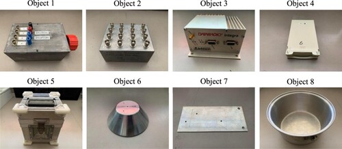Measurement of the current allowed the energy to be calculated according to Equation (22(22) $E={\int }_{-\mathrm{\infty }}^{+\mathrm{\infty }}v\left(t\right)i\left(t\right)\mathrm{d}t={\int }_0^{+\mathrm{\infty }}2|\overline{V}\left(f\right){|}^{2}G\left(f\right)\mathrm{d}f,$(22) ). The voltage maximum of each pulse was then adjusted to give pulse energy equal to 4.5 μJ. Images of the eight metallic objects used in the experiment are shown in Figure 4.

Figure 3. Electromagnetic pulse experiment setup. The cDAQ generates a voltage pulse in the transmitter coil, which creates a magnetic flux density $B_{\mathrm{coil}}$ that penetrates the metallic object and induces eddy currents. The eddy currents generate a magnetic flux density $B_{\mathrm{eddy}}$ transient that is detected by the receiver coil. The transient passes through the preamplifier and into a cDAQ analog-to-digital converter. The data is then recorded on the laptop.

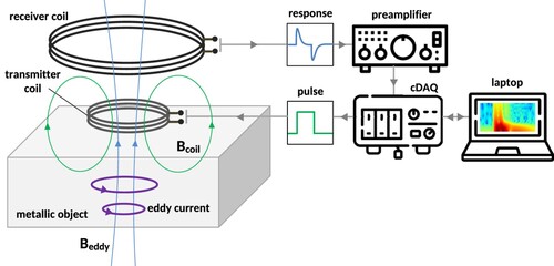
Figure 4. The eight metallic objects used in the experiment.

3.3. Data set

The transient responses for eight metallic objects were collected. Each object was placed near the sensor system with separation of between 10 and 40  mm in 5 mm increments. Additionally, the objects were shifted laterally randomly within the range 0–10  mm in the 2D plane parallel to the sensor system. At each vertical distance the experiment was replicated 100 times. As there are 8 objects, 7 distance intervals, and 6 pulse types, there are 33,600 records in total. Although the dimensions of the receiver and transmitter coil affect the magnetic field of the electromagnetic pulse, the greatest influence over classification accuracy is the signal to noise ratio (SNR), which is primarily determined by the distance between the object and the sensor system. Data collected at 10 mm have a larger SNR than data collected at 40 mm, and therefore are more likely to be correctly classified.

The transient data was collected in a 1D time domain format. The 1D data was converted into a 2D spectrogram using the MATLAB® [29] spectrogram function with frequency on the vertical axis, and time on the horizontal axis. An additional layer was added to the spectrogram data to enable the use of automated feature extraction by a CNN. Each transient data record was 30 ms duration and contained 60,000 data points. The data was downsampled to 4000 data points to limit the computational complexity of the perceptron, multiclass logistic regression, neural network and 1D CNN. The Fourier transform window was set at 3 ms duration (6000 data points) and was chosen as it is 10% of the total data set duration and fits within the beginning and end of the pulses except the rectangular pulse. The window was of the Hamming type and was chosen as it yields good sidelobe suppression and is commonly used in practice [30]. Overlaps totalled 5800. The frequency points were calculated at 8 Hz intervals between 0 Hz and 2.04 kHz (resulting in 256 vertical points in the spectrogram), where the spectrogram algorithm adds zero padding to either side of the 3 ms window before the short-time Fourier transform to achieve the required frequency resolution. The settings gave spectrogram dimensions of 256 × 271, and the final 15 columns were discarded to get a spectrogram of size 256 × 256. The training and test data set were divided according to 10-fold cross-validation.

3.4. Machine learning algorithms

A perceptron function, from the Python scikit-learn library, was used to test the linear separability of the electromagnetic pulse scattered data. The perceptron uses a stochastic gradient descent algorithm [31] as a solver with an L2 regularisation. Other inputs were $\alpha =0.0001$, maximum epochs = 5000, and stopping criterion tolerance of 0.001.

The logistic regression function from the Python scikit-learn library was used for multiclass logistic regression classification. The L-BFGS [32], a limited-memory quasi-Newton code for bound-constrained optimisation, was used as the solver with L2 regularisation with a bias added to the decision function. Other inputs were maximum epochs $=5000$, and stopping criterion tolerance of 0.0001.

Figure 5 shows an illustration of the neural network used in this work, which was created using TensorFlow [33]. The neural network has three hidden layers (4096, 128, 8) with dropout of 0.2 after the 128 node layer, a ReLU activation function on the hidden layers and a softmax function on the output layer. The model was trained for 100 epochs using a learning rate of 0.0001, a sparse categorical cross-entropy loss function, batch size of 32, and Adam optimiser.

Figure 5. Illustration of the neural network model used in this work. The input to the neural network is the time signature of the scattering response of object 8 at 10 mm from the sensor system, and is generated by a two-sided decaying exponential pulse and contains 4000 data points. This is densely connected to layer 1 with 4096 neurons and a ReLU activation function, which is connected to layer 2 with 128 neurons and a ReLU activation function. Dropout of 0.2 is applied after layer 2 and densely connected to layer 3 containing 8 neurons with a softmax function. The metallic object is classified using an argmax function.

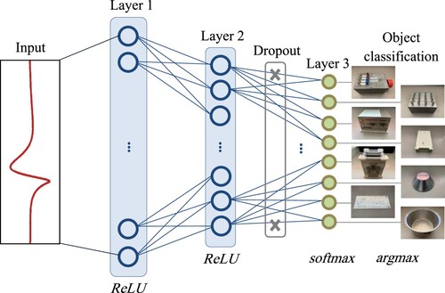
Figure 6 shows an illustration of the 1D CNN used in this work, which was created using TensorFlow. It consisted of 2 padded 1D convolutional layers of 16 filters of kernel size 64 with a ReLU activation function, a densely connected flattened layer followed by dropout of 0.2, and finally a softmax layer on 8 outputs. The learning rate was set to 0.0002, batch size of 32, Adam optimiser, and the model was trained for 100 epochs.

Figure 6. Illustration of the 1D CNN model used in this work. The input to the 1D CNN is the time signature of the scattering response of object 8 at 10 mm from the sensor system and generated by a two-sided decaying exponential pulse. Two 1D convolutional layers are used and these have the same properties – 16 filters of kernel size 64 with padding that ensures the input and output length remains constant at 4000 samples, and a ReLU activation function. These convolutional layers are stacked together and plotted as a surface in the illustration and are known as feature maps. In the feature maps red indicates large weight assigned by the 1D CNN and blue indicates small weight. The output from the second convolutional layer is flattened and densely connected to 8 neurons with a softmax activation function and the metallic object is classified using an argmax function.

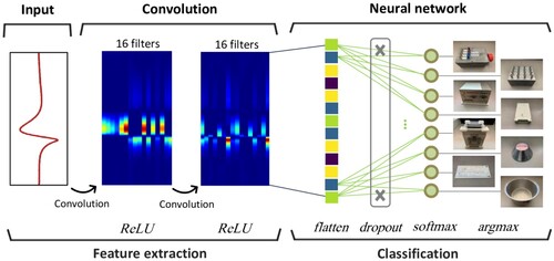
Figure 7 shows the 2D CNN used to classify the metallic objects, which was created using TensorFlow. Batch size was 32 and the Adam optimiser was used with a learning rate of 0.001. The exponential decay rate for the 1st moment (0.9) and 2nd moment (0.999) were set as the default TensorFlow values for the Adam optimiser. The model was trained for 20 epochs.

Figure 7. Illustration of the 2D CNN model used in this work. The input is a spectrogram of the scattering response of object 8 placed 10 mm from the sensor system and generated by a two-sided decaying exponential pulse. The input spectrogram has a 3 × 3 filter convolved over all pixels, and then max pooling of spatial size 2 × 2 is applied. The convolution using 3 × 3 and max pooling of 2 × 2 is repeated two times with ReLU activation functions on the output. The data is flattened and densely connected to 128 neurons with a ReLU activation function followed by dropout of 0.5. This is then connected to 8 neurons with a softmax function and finally an argmax function is applied to classify the metallic object.

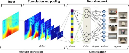
The Visual Geometry Group Network (VGGNet) [34], a deep learning algorithm that achieved high classification accuracy on the ImageNet [35] data set, uses 3 × 3 filters with 16–19 layers to reduce model size and therefore computation time. The 2D CNN model used in this work, similar to the VGGNet model, uses 32 3 × 3 filters in the convolutional layer. Filter size of 3 × 3 was chosen as it is a small size that has small computational load while providing horizontal and vertical edge detection and smoothing. There is a ReLU non-linear activation function between convolutional layers, which makes the decision function more discriminative [34]. Maximum pooling of 2 × 2 was applied after the convolutional layers to reduce the size of the model. The images were flattened into a single column array. This completes the feature extraction process. The flattened array was then densely joined to a single layer neural network of 128 nodes. Dropout was randomly applied to half of the weights to avoid overfitting [36]. A softmax function was applied to the last layer of the neural network that contains 8 classification outputs. Each classification outputs a single number where the classification chosen has the largest value.

4. Results

4.1. Time signatures

Figure 8 shows the receiver coil time signatures including reference, total, and scattered for all pulses for object 1 placed 10 mm from the sensor system. The scattered voltage equals the total voltage minus the reference voltage and is the time signature used in the perceptron, multiclass logistic regression, neural network and 1D CNN algorithms.

Figure 8. Receiver coil time signatures including reference, total, and scattered of object 1 at 10 mm for pulses (a) two-sided decaying exponential, (b) Gaussian, (c) triangular, (d) raised cosine, (e) rectangular and (f) rectangular chirp.

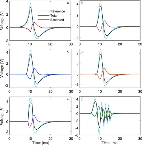
Figure 9 shows the receiver coil scattered voltage response of all objects placed 10 mm below the sensor system. Each object has a unique maximum voltage and voltage response across all pulses. On the right is a plot of the spectrogram of object 8 and is used as the input to the 2D CNN algorithm.

Figure 9. Receiver coil scattered time signatures of all objects at 10 mm, with spectrograms of object 8 to the right of the plot, for pulses (a) two-sided decaying exponential, (b) Gaussian, (c) triangular, (d) raised cosine, (e) rectangular and (f) rectangular chirp.

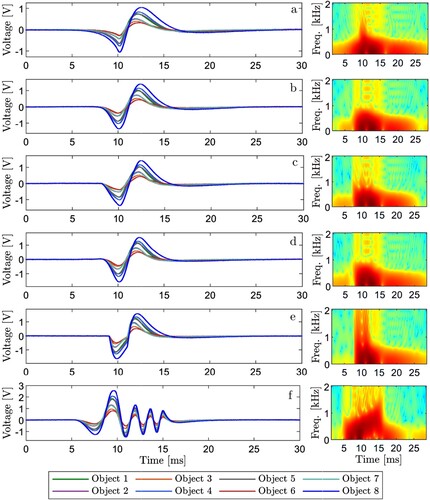
Figure 10 shows all the objects, time signatures, and spectrograms for a rectangular pulse with objects placed 10 mm from the sensor system. The bottom plot shows the scattered voltage response of the receiver coil for all objects. All objects have a unique voltage response including the maximum voltage, the time the maximum voltage occurs, the shape and decay rate. Additionally, the zero-crossing point differs between objects. For example, the voltage response of object 3 crosses zero voltage approximately 0.2 ms before object 8.

Figure 10. Object images, spectrograms, and electromagnetic scattered time signature data for the rectangular pulse. Spectrograms are expressed as power per frequency on a scale of $-30$ dB/Hz to $-140$ dB/Hz. Objects are 10 mm from the sensor system.

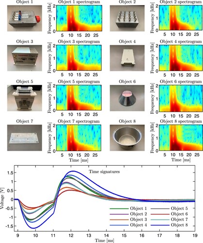
The receiver coil voltage response is a function of the size and shape of the metallic object. Object 7, a plate, has a larger voltage maximum than object 6, a truncated cone, but decays faster. The plate is thin and does not sustain lower frequencies in the bulk of the material, whereas the truncated cone has much more volume and this is reflected in a sustained voltage response of low frequency components of the rectangular pulse.

4.2. Classification accuracy

Classification accuracy of the 10-fold cross-validation for each pulse and classifier is shown in Figure 11. Each circle marker corresponds to an accuracy for a single fold, thereby displaying the distribution of the 10-fold cross-validation. The minimum, maximum, first quartile, third quartile, and median are also shown.

Figure 11. Machine learning classification results for each pulse and classifier. Each circle marker is a classification accuracy in the 10-fold cross-validation. The minimum, maximum, first quartile, third quartile, and median are also shown. Note that the perceptron has a different horizontal scale for illustration purposes.

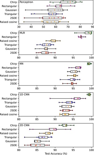
The perceptron has the largest median classification accuracy of 71.7% for the rectangular chirp pulse, and lowest median of 56.4% for the raised cosine pulse. The low classification accuracy across all pulses indicates that the electromagnetic pulse scattered data is not linearly separable.

The multiclass logistic regression (MLR in the plot) has the largest median classification accuracy of 99.6% for the rectangular chirp pulse (although the mean is lower at 98.8%), closely followed by 97.1% for the rectangular pulse. The lowest median accuracy of 87.5% is the two-sided decaying exponential pulse. The large median classification accuracy of the rectangular chirp and rectangular pulse suggests that for these pulses a linear model is sufficient for large classification accuracy of the metallic objects used in this work. This may be attributable to the higher frequency components present in both the chirp and rectangular pulses, which provide information about the objects including shape, relative to the other pulses.

The neural network (NN in the plot) has the largest median classification accuracy of 99.3% for the rectangular chirp pulse, which is less than the multiclass logistic regression, however the neural network has lower standard deviation of 0.4% versus 1.8%. The neural network classifier resulted in a significant improvement in median classification accuracy for the Gaussian (+8.1%), triangular (+7.5%), two-sided decaying exponential (+7.2%), and raised cosine (+5.7%) pulses, and a decrease in median classification accuracy for the rectangular (−0.8%) and chirp (−0.3%) pulses. This suggests that a non-linear classifier is required to achieve large classification accuracy for the Gaussian, triangular, two-sided decaying exponential, and raised cosine pulses.

The 1D CNN has the largest median classification accuracy of 99.5% for the chirp pulse, which is less than the multiclass logistic regression, however the 1D CNN has lower standard deviation of 0.3% versus 1.8%. The 1D CNN median classification accuracy was larger than the neural network for the rectangular chirp pulse, but underperformed all other pulses.

For the 2D CNN classifier, the rectangular chirp is the best performing pulse with a mean classification accuracy exceeding the next best performing pulse, the rectangular pulse, by 3.8 percent on average over 10-fold cross-validation data. The lowest classification accuracy of the chirp is larger than the upper quartile of the rectangular pulse, and larger than the largest classification accuracy of all other pulses.

The rectangular chirp mean classification accuracy exceeds the two-sided decaying exponential, the worst performing pulse, by 7.9 percent on average over 10-fold cross-validation data. The rectangular chirp possibly outperforms the other pulses due to having a greater amount of energy in the higher frequency part of its spectrum. The chirp also has a more uniform distribution of energy across the spectrum compared to the other pulses, which are mostly concentrated in the lower frequency part of the spectrum. Higher frequencies penetrate a shallower depth through the objects due to the skin effect. The chirp may be effective at evoking strong eddy currents at the surface of the metallic objects, revealing additional information not present in other pulses. The chirp also has greater pulse duration and zero-crossing points compared to the other pulses.

Figure 12 shows a heatmap table of mean classification accuracy and standard deviation for all pulses and classifiers. The rectangular chirp pulse has the largest, and equal, mean accuracy for the 1D CNN (99.4 ± 0.3%) and neural network (99.4 ± 0.4%) classifiers, although the 1D CNN has a lower standard deviation. The 1D CNN underperforms the neural network for all other pulse types.

Figure 12. Mean classification accuracy and standard deviation (%) over 10-fold cross-validation for all pulses and classifiers.

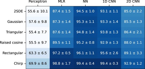
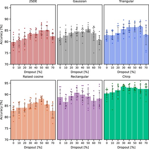
Figure 13 shows a plot of classification accuracy versus dropout percentage for 10-fold cross-validation and the 2D CNN, where dropout is used in the model according to Figure 7. The bar plot is the mean classification accuracy of the 10-folds, the error bars are the standard deviation, and the circle markers indicate each of the 10 data points for each dropout percentage. All pulses have a dropout percentage that maximises the classification accuracy and these are two-sided decaying exponential (60%), Gaussian (50%), triangular (60%), raised cosine (50%), rectangular (30%), and rectangular chirp (30%).

Figure 13. Dropout versus classification accuracy where bars are mean classification accuracy, error bars are the standard deviation, and circle markers indicate the classification accuracy of each fold in the 10-fold cross-validation.

4.3. Confusion matrices

A confusion matrix for each pulse and classifier, with classification output summed over all 10-fold cross-validation data points, is given in Figure 14.

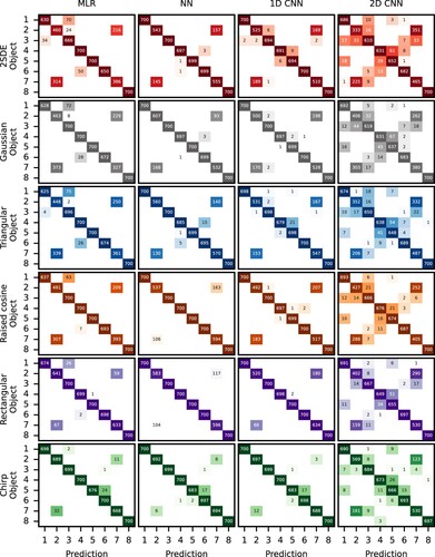
The multiclass logistic regression confuses objects 2–7 across all pulses. All pulses confuse objects 1–3, however, the rectangular chirp pulse only does this 2 times compared to 79 times for the triangular pulse. Although the rectangular chirp pulse has the largest mean classification accuracy, it does confuse objects 5–6 24 times, whereas no other pulse type confuses objects 5–6.

Figure 14. Confusion matrices of summed 10-folds for all pulses and classifiers.

The neural network improves classification accuracy compared to the multiclass logistic regression, except for the rectangular pulse. Despite being a non-linear algorithm, the objects confused (primarily 2–7) are very similar to the linear multiclass logistic regression. One difference is object 1–3, which is never confused by the neural network classifier whereas the multiclass logistic regression confuses these objects for all pulses.

The 1D CNN classifier has performance comparable to the neural network classifier where objects 2–7 are often confused. One notable difference is for the triangular pulse where the 1D CNN often confuses objects 4–5 whereas the neural network often confuses objects 4–6.

The 2D CNN confuses many more objects compared to the multiclass logistic regression, neural network, and 1D CNN. Large classification errors were observed for object pairs 2–3, 4–5, and 2–7. The rectangular chirp had the largest mean accuracy, and this was achieved by accurately classifying objects 2–7 relative to the other pulses. The two-sided decaying exponential pulse, the worst performing pulse, incorrectly classified objects 2–7 576 times. The rectangular chirp incorrectly classified objects 2–7 284 times, a substantial improvement over the two-sided decaying exponential pulse. Interestingly, the mean classification error order of pulses is also the same order of accuracy of classifying objects 2–7. The rectangular chirp is able to significantly outperform other pulses in distinguishing between objects 2–7. While the rectangular chirp performs best at classifying objects 2–7, it underperforms other pulses for different objects. The rectangular pulse, for example, does not confuse objects 5–6. The rectangular chirp, however, confuses objects 5–6 a total of 21 times. All pulses, excluding the rectangular chirp with 3 incorrectly classified objects, were able to correctly classify object 8. This suggests that some pulses, while having a lower mean accuracy, may be used for the purpose of distinguishing between two specific objects. For example a rectangular pulse may be used to distinguish between objects 5–6.

4.4. Feature maps

Feature maps assist in the interpretation of the hidden layers of a CNN. Visualisation of the neuron activation levels at the end of the convolution layers provides insight into the abstracted features that were used by the CNN for classification.

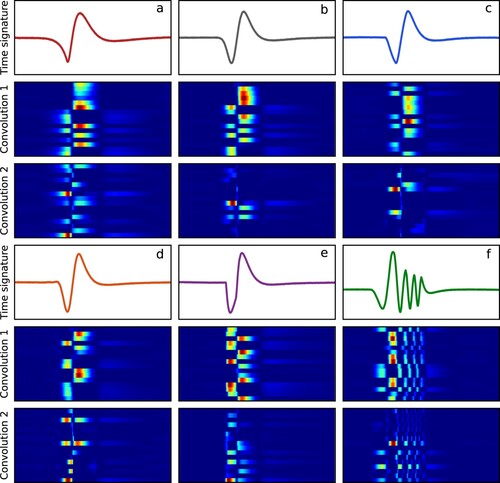
Feature maps of all the pulses for the 1D CNN classifier and object 8 at 10 mm are shown in Figure 15. All pulses have large weights at and around the minimum and maximum voltage of the time signature. The rectangular chirp pulse has largest weight at the second peak for convolutional layer 1 and 2, which corresponds to low to medium frequencies used in the pulse (the chirp is unique in that it has a strict relationship between frequency and time). This part of the signal also corresponds to the largest SNR in the chirp and may be an influencing factor in the weights assigned by the 1D CNN. There is also weight applied to the high frequency parts of the chirp time signature, indicating that both low and high frequencies are used for classification.

Figure 15. Receiver coil scattered time signatures of object 8 at 10 mm, and the first and second convolutional layer feature maps, for pulses (a) two-sided decaying exponential, (b) Gaussian, (c) triangular, (d) raised cosine, (e) rectangular and (f) rectangular chirp. In the feature maps red signifies large weight and blue signifies small weight in the 1D CNN.

A subset of feature maps for all electromagnetic pulses and the 2D CNN classifier for object 8 at 10 mm are shown in Figure 16. In the feature maps red signifies large weight and blue signifies small weight in the 2D CNN. The spectrogram plots (labelled a–f) show the input to the 2D CNN.

Figure 16. Spectrogram input and a subset of 2D CNN feature maps of convolutional layers for object 8 placed 10 mm above the sensor system for pulses: (a) two-sided decaying exponential, (b) Gaussian, (c) triangular, (d) raised cosine, (e) rectangular and (f) rectangular chirp. In the feature maps red signifies large weight and blue signifies small weight in the 2D CNN.

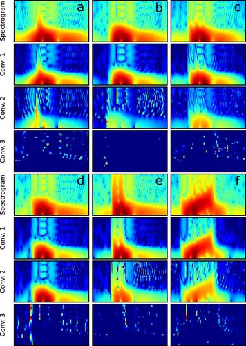
The first convolutional layer (Conv. 1), corresponding to the structure shown in Figure 7, shows high level features of the spectrogram used by the 2D CNN. This includes placing low weight (blue colour in plot) on noise, and placing large weight (red colour in plot) on the early time and low frequency part of the spectrogram across all pulses. For all pulses, the late time part of the spectrogram (after 15 ms) has moderate weight assigned to the low frequency part of the spectrogram.

The second convolutional layer (Conv. 2) shows mid-level features with large weights. In the case of the two-sided decaying exponential pulse, large weight has been assigned to the early and high frequency part of the spectrogram, and to two small low frequency areas of the spectrogram. The chirp has largest weight on the low frequency part, and moderate weight on the high frequency part, of the spectrogram. Similar weights were applied by the 1D CNN classifier to the low and high frequency parts of the rectangular chirp time signature.

Low level features in the third convolutional layer (Conv. 3) are sparse due to max pooling, but generally appear to be focussed around the envelope of the input spectrogram.

5. Conclusions

In this paper metallic objects were classified using linear (perceptron and multiclass logistic regression) and non-linear (neural network, 1D CNN, and 2D CNN) machine learning algorithms. Several electromagnetic pulses, including a two-sided decaying exponential, Gaussian, triangular, raised cosine, rectangular, and rectangular chirp, were used.

All electromagnetic pulses were able to classify metallic objects to differing degrees. The perceptron classifier had maximum mean classification accuracy of 69.9 ± 8.6% for the rectangular chirp pulse, with all other pulses being less accurate, indicating that the electromagnetic pulse scattered data is not linearly separable. The largest mean classification accuracy, with the lowest standard deviation, was 99.4 ± 0.3% for the rectangular chirp pulse and the 1D CNN classifier.

In the case of the 2D CNN, the two-sided decaying exponential pulse was the worst performing pulse with a mean classification accuracy of 85.0 ± 2.2%. The rectangular chirp was the best performing pulse with a classification accuracy of 92.9 ± 1.2%. Although the rectangular chirp was the best performing pulse, it did not classify every object pair better than all other pulses. In particular, the rectangular pulse outperformed the rectangular chirp pulse when classifying objects 5–6.

Feature maps were presented and large weights on the low frequency, short time section of the spectrogram indicates that this was an important feature used by the 2D CNN for classification. The rectangular chirp pulse had large weight at low frequencies, and moderate weight at high frequencies for both the 1D CNN and 2D CNN classifiers.

The possible applications of this work are multiple. Metallic object classification has uses in threat object classification and metallic waste object sorting. Classification algorithms, such as the CNN, which are able to automate feature extraction, promise to reduce human involvement in metallic object detection.

While results are promising, further work on classification of metallic objects submerged in dielectrics such as water, and weak conductors such as sand and seawater, will provide insight into the effectiveness of different pulses in different environmental conditions. Environmental effects will alter the pulse shape, and the electromagnetic field and matter interaction, introducing additional effects that may reduce classification accuracy.

A bespoke 2D CNN, with 3 convolutional layers, was used in this work and its feature maps were illustrated for explainability purposes. Further investigation of well known 2D CNN deep learning algorithms such as VGGNet, Inception-V3 [37], and Residual Networks (ResNet) [38] may result in larger classification accuracy and overcome any of the potential shortcomings of the bespoke 2D CNN used in this work.

Disclosure statement

No potential conflict of interest was reported by the author(s).

References

- Wilson BA, Ledger PD, Lionheart WR. Identification of metallic objects using spectral magnetic polarizability tensor signatures: object classification. Int J Numer Methods Eng. 2022;123(9):2076–2111. doi: 10.1002/nme.v123.9
- Dang TL, Cao T, Hoshino Y. Classification of metal objects using deep neural networks in waste processing line. Int J Innov Comput Inf Control. 2019;15(5):1901–1912.
- Ge J, Yusa N, Fan M. Frequency component mixing of pulsed or multi-frequency eddy current testing for nonferromagnetic plate thickness measurement using a multi-gene genetic programming algorithm. NDT E Int. 2021;120:Article ID 102423. doi: 10.1016/j.ndteint.2021.102423
- Yan B, Li Y, Liu Z, et al. Pulse-modulation eddy current imaging and evaluation of subsurface corrosion via the improved small sub-domain filtering method. NDT E Int. 2021;119:Article ID 102404. doi: 10.1016/j.ndteint.2021.102404
- Li Y, Yan B, Li W, et al. Pulse-modulation eddy current probes for imaging of external corrosion in nonmagnetic pipes. NDT E Int. 2017;88:51–58. doi: 10.1016/j.ndteint.2017.02.009
- Zhu P, Cheng Y, Banerjee P, et al. A novel machine learning model for eddy current testing with uncertainty. NDT E Int. 2019;101:104–112. doi: 10.1016/j.ndteint.2018.09.010
- Bai L, Gao B, Tian S, et al. A comparative study of principal component analysis and independent component analysis in eddy current pulsed thermography data processing. Rev Sci Instrum. 2013;84(10):Article ID 104901. doi: 10.1063/1.4823521
- Sophian A, Tian GY, Taylor D, et al. A feature extraction technique based on principal component analysis for pulsed eddy current NDT. NDT E Int. 2003;36(1):37–41. doi: 10.1016/S0963-8695(02)00069-5
- Šimić M, Ambruš D, Bilas V. Landmine identification from pulse induction metal detector data using machine learning. IEEE Sens Lett. 2023;7(9):1–4.
- Krizhevsky A, Sutskever I, Hinton GE. ImageNet classification with deep convolutional neural networks. In: Advances in neural information processing systems. Vol. 25; 2012.
- Goodfellow I, Bengio Y, Courville A. Deep learning. Cambridge: MIT Press; 2016.
- Luo Q, Gao B, Woo WL, et al. Temporal and spatial deep learning network for infrared thermal defect detection. NDT E Int. 2019;108:Article ID 102164. doi: 10.1016/j.ndteint.2019.102164
- Miorelli R, Fisher C, Kulakovskyi A, et al. Defect sizing in guided wave imaging structural health monitoring using convolutional neural networks. NDT E Int. 2021;122:Article ID 102480. doi: 10.1016/j.ndteint.2021.102480
- Ye J, Ito S, Toyama N. Computerized ultrasonic imaging inspection: from shallow to deep learning. Sensors. 2018;18(11):3820. doi: 10.3390/s18113820
- Salucci M, Anselmi N, Oliveri G, et al. A nonlinear kernel-based adaptive learning-by-examples method for robust NDT/NDE of conductive tubes. J Electromagn Waves Appl. 2019;33(6):669–696. doi: 10.1080/09205071.2019.1572546
- Thomas R, Salmon B, Holloway D, et al. Machine learning classification of metallic objects using pulse induction electromagnetic data. Meas Sci Technol. 2024;35(6):Article ID 066103. doi: 10.1088/1361-6501/ad2cdd
- Jiang W, Ren Y, Liu Y, et al. Artificial neural networks and deep learning techniques applied to radar target detection: a review. Electronics. 2022;11(1):156. doi: 10.3390/electronics11010156
- Wang C, Wang J, Zhang X. Automatic radar waveform recognition based on time-frequency analysis and convolutional neural network. In: 2017 IEEE International Conference on Acoustics, Speech and Signal Processing (ICASSP). IEEE; 2017. p. 2437–2441.
- Gao J, Lu Y, Qi J, et al. A radar signal recognition system based on non-negative matrix factorization network and improved artificial bee colony algorithm. IEEE Access. 2019;7:117612–117626. doi: 10.1109/Access.6287639
- Ding J, Chen B, Liu H, et al. Convolutional neural network with data augmentation for SAR target recognition. IEEE Geosci Remote Sens Lett. 2016;13(3):364–368.
- Dong X, Zhao Z, Wang Y, et al. FMCW radar-based hand gesture recognition using spatiotemporal deformable and context-aware convolutional 5-D feature representation. IEEE Trans Geosci Remote Sens. 2021;60:1–11.
- Chen H, Ye W. Classification of human activity based on radar signal using 1-D convolutional neural network. IEEE Geosci Remote Sens Lett. 2019;17(7):1178–1182. doi: 10.1109/LGRS.8859
- Arfken GB, Weber HJ. Mathematical methods for physicists. Boston: Academic Press; 2013.
- Grami A. Introduction to digital communications. Boston: Academic Press; 2015.
- Kelkar S, Grigsby L, Langsner J. An extension of Parseval's theorem and its use in calculating transient energy in the frequency domain. IEEE Trans Ind Electron. 1983;IE-30:42–45. doi: 10.1109/TIE.1983.356702
- Ward SH, Hohmann GW. Electromagnetic theory for geophysical applications. In: Electromagnetic methods in applied geophysics. Vol. 1. Theory. Society of exploration geophysicists; 1988. p. 130–311.
- Burke SK, Ibrahim M. Electrical and magnetic properties of D6ac steel. Melbourne: Defence Science and Technology Organisation; 2007.
- Shackelford JF, Alexander W. CRC materials science and engineering handbook. Boca Raton: CRC Press; 2000.
- The MathWorks Inc. MATLAB version: 9.11.0.1769968 (R2021b); 2021. Available from: https://www.mathworks.com
- Harris FJ. On the use of windows for harmonic analysis with the discrete Fourier transform. Proc IEEE. 1978;66(1):51–83. doi: 10.1109/PROC.1978.10837
- Bottou L. Stochastic gradient learning in neural networks. In: Proceedings of Neuro-Nımes. Vol. 91(8). Nimes; 1991. p. 12.
- Byrd RH, Lu P, Nocedal J, et al. A limited memory algorithm for bound constrained optimization. SIAM J Sci Comput. 1995;16(5):1190–1208. doi: 10.1137/0916069
- Abadi M, Agarwal A, Barham P, et al. TensorFlow: large-scale machine learning on heterogeneous systems; 2016. arXiv:160304467.
- Simonyan K, Zisserman A. Very deep convolutional networks for large-scale image recognition; 2014. arXiv preprint arXiv:14091556.
- Deng J, Dong W, Socher R, et al. ImageNet: a large-scale hierarchical image database. In: 2009 IEEE Conference on Computer Vision and Pattern Recognition. IEEE; 2009. p. 248–255.
- Srivastava N, Hinton G, Krizhevsky A, et al. Dropout: a simple way to prevent neural networks from overfitting. J Mach Learn Res. 2014;15(1):1929–1958.
- Szegedy C, Vanhoucke V, Ioffe S, et al. Rethinking the inception architecture for computer vision. In: Proceedings of the IEEE Conference on Computer Vision and Pattern Recognition; 2016. p. 2818–2826.
- He K, Zhang X, Ren S, et al. Deep residual learning for image recognition. In: Proceedings of the IEEE Conference on Computer Vision and Pattern Recognition; 2016. p. 770–778.