Simulating the induction heating of cross-ply C/PEKK laminates – sensitivity and effect of material variability

Abstract

A simulation model for the induction heating of UD tape-based thermoplastic composites is presented in this work. The model is based on the electrical ply properties which were determined experimentally for two commercially available carbon reinforced tape materials. Moreover, the interrelation between the measured electrical conductivities and the fiber distribution in the tape and laminates is discussed based on microscopic structure evaluation. The model was validated experimentally for the induction heating of cross-ply laminates. Subsequently, the effect of the experimental variability in the measured conductivities on the heating behavior was investigated using the simulation model. It was found that the material variability can have a significant effect on the heating behavior.

Keywords:

• thermoplastic composites
• induction heating
• electrical conductivity
• experiments
• modeling

1. Introduction

Ever since their introduction in the 1980s, thermoplastic composite materials are increasingly being applied in commercial aircraft. Initially, the applications were limited to smaller secondary components, but today thermoplastic composites are also considered for larger primary structures, such as fuselage sections [1] or engine pylons [2], with recent advances in 3D printing providing additional opportunities for part production [3–5]. Large aerostructures are typically assembled from smaller components. Here, the weldability of thermoplastic composites provides them a key advantage over their thermoset counterparts, sidestepping disadvantages associated with fastening and adhesive bonding [6,7].

Of the available welding technologies, induction welding is particularly attractive for carbon fiber reinforced thermoplastics as it does not require a susceptor material at the weld interface. The process relies on an alternating magnetic field to generate heat in the carbon fiber reinforced thermoplastic adherends in order to fuse them together [8–10]. The underlying heating mechanisms are Joule heating in the carbon fibers and in the fiber-fiber contacts, and dielectric heating at the fiber junctions [8,9,11–13]. Irrespective of the heating mechanism, induction heating requires the presence of eddy currents in the material [8,9]. Eddy currents are relatively easily generated in woven fabric composites, where the interlacement of bundles facilitates contact between perpendicular fibers to provide a conductive loop. This is not the case for composites based on unidirectional (UD) tape materials. The highly anisotropic nature of UD plies, which have a very low transverse electrical conductivity, hinders eddy current formation in a ply. Instead, the ability to form eddy currents in UD laminates depends on the through-thickness ply conductivity and the contact resistance at the interfaces between plies with different fiber orientations [14,15].

Induction welding of fabric reinforced thermoplastics has a reached a high technology readiness level and is currently successfully applied by GKN/Fokker for the assembly of the rudder and elevator of the Gulfstream G650 [16]. The process, however, still relies on extensive welding trials to develop a processing window that provides full interlaminar bonding, while preventing degradation and achieving the required level of crystallinity [17]. Additionally, the process is sensitive to local variations in fiber volume fraction and fiber distribution because the degree of fiber to fiber contact affects the ability to form eddy currents. The latter is particularly true for laminates based on UD tape materials which, as was mentioned earlier, have a very low transverse conductivity. Predictive process simulations could help to reduce the time and costs required for process development, while they also provide means for process optimization in terms of robustness.

Simulation of induction heating of continuous carbon fiber composites has received relatively little attention. Most of the approaches mentioned in literature consider woven fabric reinforced laminates, e.g. [18–21], while only a few works specifically considered UD tape reinforced laminates. Bensaid et al. and Wasselnyck et al. presented a finite element shell formulation in a series of IEEE contributions [15,22,23] that was also used to simulate the induction heating of UD tape-based laminates. The proposed formulation, however, cannot account for the through-thickness current. The effect of the ply interfaces was considered through the definition of an interphase region with in-plane electrical conductivities equal to the average conductivity of its adjacent plies [15]. Despite this simplification, decent agreement was found between the experimental and simulation results, although details on the thickness of the interphase region and the material used for experimental validation were not reported. More recently, O’Shaughnessey et al. modeled the induction heating of UD carbon polyphenylenesulphide laminates with a metal susceptor mesh at the weld interface using Comsol® [24]. The authors determined the in-plane electrical conductivities of the laminated adherends, as opposed to the ply properties, at room temperature using the four-probe method, while the through-thickness conductivity was estimated using micromechanics. The in-plane conductivity values were extrapolated for higher temperatures, whereas this was not the case for the through-thickness conductivity. These authors also reported good agreement between the model and the experiments.

The present work considers the induction heating of UD tape-based cross-ply C/PEKK laminates. More specifically, it addresses the sensitivity of the induction heating process to variations in the material’s electrical conductivities. For this purpose, a simulation approach for UD tape-based thermoplastic composites is proposed following the work of for example O’Shaughnessey et al. [24]. The approach here, however, is based on the ply properties instead of the homogenized laminate properties, providing greater flexibility for optimization. The required anisotropic ply conductivities were characterized experimentally for carbon polyetherketoneketone (C/PEKK) tape materials from two suppliers. The model was validated by comparing the simulation results with experimentally obtained time vs. temperature curves, while the effect of small variations on the conductivities was investigated in a sensitivity analysis. Finally, the effect of variability in the measured conductivities on the heating rate was studied and discussed.

2. Experimental work

2.1. Materials, lay-up and consolidation

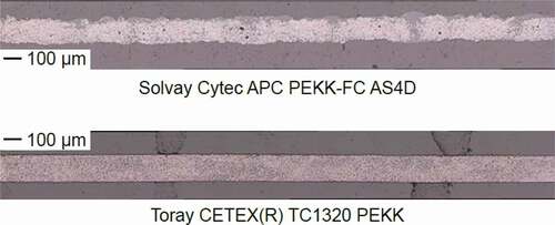
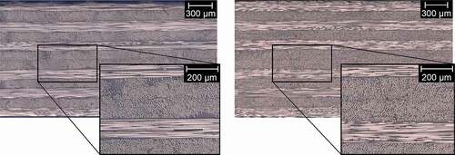
Unidirectional carbon fiber reinforced polyetherketoneketone (C/PEKK) prepreg tape materials from two suppliers were used in this work, namely Solvay (Cytec APC PEKK-FC/AS4D) and Toray (Cetex® TC1320 PEKK). Both tape materials employ a 12K AS4D carbon fiber from Hexcel, have a fiber areal weight of 145 g/m², are based on a PEKK polymer, and have a resin mass content of 34%. The morphologies of the tapes differ significantly as can be seen from the micrographs of the as-received tapes shown in Figure 1. The tape from Toray shows a homogeneous fiber distribution and smooth surfaces. The fiber distribution in the tape from Solvay is more inhomogeneous with resin rich regions between clusters of bundles, while also its surfaces are irregular compared to the tape from Toray.

Figure 1. Cross-sectional micrographs of the as-received tape materials

The induction heating experiments were performed on cross-ply laminates having a [0/90]_3s lay-up. After the induction heating experiments, specimens were cut from the cross-ply laminates for the purpose of measuring the through-thickness electrical conductivity. Additionally, three 108-ply unidirectional (UD) laminates, i.e. having a [0]₁₀₈ lay-up, were manufactured from each material system for the in-plane electrical conductivity experiments.

The laminates were consolidated in a static consolidation press. A 305 × 305 mm² picture frame mold was used for the cross-ply laminates while a 100 × 100 mm² picture frame was used for the UD laminates. The picture frame mold was heated to a temperature of 375 °C, as measured using a thermocouple in the stack, consolidated for 20 minutes and subsequently cooled down to room temperature at a rate of 4.5°C/min. Following the instructions of the material suppliers, the Toray laminates were consolidated at a pressure of 20 bar, while the Solvay laminates were consolidated at a pressure of 7 bar. The laminates were inspected non-destructively after manufacturing using ultrasound and no voids or defects were found. The average thickness of the Solvay and Toray cross-ply laminates equalled 1.65 mm and 1.73 mm, respectively, while the Solvay UD laminates had an average thickness of 14.52 mm compared to 15.39 mm for the Toray UD laminates.

2.2. Static induction heating experiments

Static induction heating experiments were performed on the two single cross-ply laminates. The laminates were cut to dimensions of 290 × 290 mm² prior to the heating experiments, in order to prevent any edge damage effects and to ensure equal laminate size. Moreover, the laminates were dried overnight in a convection oven at 160 °C.

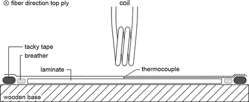
The experimental setup is illustrated in Figure 2. A 15 mm thick compressed high-pressure wooden laminate was used as a base. It was selected because it is transparent to the electromagnetic field and can withstand the high temperatures. The C/PEKK laminate was then fixed onto the base plate using a vacuum bag in order to ensure proper contact between the base plate and the laminate. A welded E-type thermocouple, having a diameter of 0.13 mm, was placed at the center on the top surface of the laminate. The coil was placed above the center of the laminate, and thus directly above the thermocouple. A spacer block of 12.4 mm was used to ensure a fixed and repeatable distance between the coil and the laminate. The fiber direction of the top ply was aligned parallel to the windings of the coil.

Figure 2. Schematic illustration of the induction heating setup

An Ambrel EASYHeat 8310 LI induction heating system with a 10 kW power output, a frequency range between 150 and 400 kHz and a maximum current of 750 A, was used to provide the current for the coil. The copper coil itself was cylindrical and had three full windings, an inner diameter of 32.5 mm, a pitch of 6.1 mm and a tube outer diameter of 4.8 mm. A constant coil RMS current of 350 A at a frequency of 275 kHz was used to heat the laminates to approximately 250°C, after which the current was switched off for the laminate to cool to room temperature. The surface temperature was recorded using the thermocouple. The experiment was replicated four times, without removing the laminate from the vacuum bag.

2.3. Conductivity experiments

Specimens for the conductivity experiments were cut from the thick UD laminates using a water-cooled diamond-coated saw. The specimens for the in-plane conductivity measured 80 × 16 mm², while the through-thickness specimens measured 16 × 16 mm². Additionally, specimens for through-thickness conductivity measurements were also cut from the cross-ply laminates after the induction heating experiments.

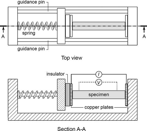
A special purpose set-up, as schematically illustrated in Figure 3, was developed to perform the conductivity measurements. The specimens were clamped between two copper plates. A spring was used to provide the needed contact force, while, in addition, silver paste was used between the specimen and the copper contact plate to ensure electrical contact. The in-plane conductivity in fiber direction was characterized using the four-probe method, which is based on the measurement of the potential drop between two points on the specimen, while a fixed current is applied. The four-probe method is suited for highly conductive materials, such as carbon fibers, as lead and contact resistance can be neglected [25]. The in-plane conductivity transverse to the fiber direction and the out-of-plane conductivity were obtained using the two-probe method. Each measurement was performed twice, and five specimens were tested for each sample. The current direction was changed in the second measurement to eliminate contact potential, as specified in ASTM B193-16.

Figure 3. Schematic illustration of the setup used to characterize the electrical conductivity

3. Experimental results

3.1. Induction heating experiments

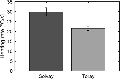
Figure 4 shows the surface temperature directly under the coil for the two cross-ply laminates as measured using the thermocouple. The graph shows that the temperature evolution is different for the two material systems. This influence is also illustrated in Figure 5, which shows the averaged heating rate at 75 °C. Clearly, the laminate from Solvay heats up faster than the laminate from Toray.

Figure 4. Average laminate temperature directly under the coil as measured by the thermocouple. The error bars represent the standard deviation of four measurements. The error bars are only plotted for every 5th data point for clarity

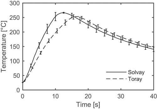
Figure 5. Averaged heating rate and standard deviation at 75°C

3.2. Conductivity measurements

Table 1 and Figure 6 show the measured electrical conductivity in fiber direction σ₀, perpendicular to the fiber direction σ₉₀ and in the through-thickness direction σ_z for the UD C/PEKK laminates, while the last column shows the through-thickness conductivity σ_z for the cross-ply laminates. As expected, the conductivity is highly anisotropic, with approximately five orders of magnitude difference between the conductivity in fiber and the through-thickness direction.

Figure 6. The electric conductivities as measured from the UD laminates and the through-thickness electric conductivity σz for the cross-ply layups

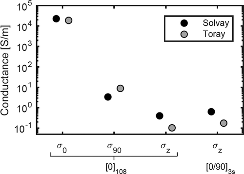
Table 1. Electrical conductivity of C/PEKK from Solvay and Toray

	UD laminates [0]108						Cross-ply [0/90]3s
	σ0 [S/m]		σ90 [S/m]		σz [S/m]		σz [S/m]
	Mean	Std	Mean	Std	Mean	Std	Mean	Std
Solvay	2.29∙10^4	0.05∙10^4	3.37∙10°	0.06∙10°	4.00∙10^−1	2.20∙10^−1	6.36∙10^−1	3.11∙10^−1
Toray	1.89∙10^4	0.18∙10^4	8.83∙10°	0.28∙10°	1.03∙10^−1	0.15∙10^−1	1.75∙10^−1	0.27∙10^−1

Although the conductivities for the two different materials are in the same order of magnitude, there are some differences. Firstly, the Solvay material has a higher conductivity in fiber direction ${\sigma }_0$ than the Toray material, that is 2.3∙10⁴ S/m versus 1.9∙10⁴ S/m, respectively. For sake of reference, the theoretical value for ${\sigma }_0$ can be determined using a rules of mixture approach. The electrical conductivity of the AS4 fiber equals 5.9∙10⁴ S/m [26], whereas the electrical conductivity of PEKK is negligible having a value in the order of magnitude of 10⁻¹⁴ S/m [27]. The theoretical electrical conductivity of a ply in fiber direction can then be estimated as approximately 3.5∙10⁴ S/m using a fiber volume fraction of 0.59. The experimentally determined values are quite a bit lower than the estimated theoretical value, i.e. approximately 35% for Solvay and 45% for Toray. Secondly, the tape from Toray shows a higher in-plane transverse conductivity compared to the Solvay tape, while the opposite holds for the through-thickness conductivity. The difference in out-of-plane conductivity between the two materials may, however, not be regarded as significant, given the high standard deviation for the out-of-plane Solvay specimens shown in Table 1. Lastly, the through-thickness data of the thick UD laminate is comparable to that of the cross-ply laminate, suggesting that the effect of the interfaces is small. Given the large standard deviation on the through-thickness data, as listed in Table 1, it is difficult to draw definitive conclusions, however.

The standard deviations indicate a large variability in the data for some of the conductivities. Most notably, the coefficient of variation (CoV) for the through-thickness conductivity is particularly high. The Solvay samples show a CoV for the through-thickness conductivity of 0.55 and 0.48 for the UD and cross-ply laminates, respectively, compared to a value of 0.02 for the in-plane conductivities. The difference in between the CoV of in-plane and through-thickness conductivity is less pronounced for the Toray samples, which shows a coefficient of variation for the through-thickness conductivity of approximately 0.15 for both the UD as the cross-ply laminate, compared to a CoV for the in-plane conductivities of 0.10 in fiber direction and 0.03 transverse to the fiber direction. The influence of the variability in the material property data will be investigated with help of induction heating simulations elaborated in the next section.

4. Simulation model

4.1. Governing equations

The present section introduces the governing equations for the electromagnetic and thermal domain in generic terms. The electromagnetic field is calculated using Maxwell’s equations, which comprise:

Gauss’s law:

(1) $\mathrm{\nabla }\cdot E=\rho ,$(1)

Gauss’s law for magnetism:

(2) $B={\mu }_0{\mu }_{\mathrm{r}}H$(2)

The Maxwell-Faraday equation:

(3) $\mathrm{\nabla }\times E=-\frac{\mathrm{\partial }B}{\mathrm{\partial }t},$(3)

and Ampère’s circuital law:

(4) $\mathrm{\nabla }\times H=J+\frac{\mathrm{\partial }D}{\mathrm{\partial }t},$(4)

in which is $\rho$ the electric charge density, $E$ is the electric field, $B$ is the magnetic induction, $D$ is the electric flux density, $J$ denotes the electric current density and $H$ represents the magnetic field, while time is denoted with $t$. The Maxwell equations are complemented with the following constitutive equations:

(5) $D={ϵ}_0{ϵ}_{r}E,$(5)

(6) $B={\mu }_0{\mu }_{\mathrm{r}}H$(6)

(7) $J=\stackrel{=}{\sigma }\cdot E,$(7)

in which ${ϵ}_0$ represents the absolute permittivity, ${ϵ}_{\mathrm{r}}$ the relative electric permittivity, ${\mu }_0$ is the magnetic constant, ${\mu }_{\mathrm{r}}$ the relative magnetic permeability and $\mathrm{\nabla }\times A=B$ is the conductivity tensor, which was determined experimentally in the previous section.

The temperature distribution in the laminate is governed by the heat equation:

(8) $\rho c_{\mathrm{p}}\frac{\mathrm{\partial }T}{\mathrm{\partial }t}-\mathrm{\nabla }\cdot \left(\stackrel{=}{\lambda }\mathrm{\nabla }T\right)=\dot{\mathrm{Q}}$(8)

with the density, $c_{\mathrm{p}}$ the specific heat, the thermal conductivity tensor and $\dot{\mathrm{Q}}$ heat generation rate as a result of Joule heating which equals:

(9) $\dot{\mathrm{Q}}={\mathbf{J}}^T\cdot \stackrel{-1}{\stackrel{=}{\sigma }}\cdot \mathbf{J}$(9)

4.2. Model

A Comsol Multiphysics® model was developed to simulate the induction heating of the cross-ply laminates. The electromagnetic problem, Equations (1)(1) $\mathrm{\nabla }\cdot E=\rho ,$(1) –(7), was solved in the frequency domain using the Magnetic Fields (MF) module. Once the current distribution was obtained, a transient thermal model was solved using the Heat Transfer (HT) in solids module. The Multiphysics couplings add the electromagnetic power dissipation, Equation (9)(9) $\dot{\mathrm{Q}}={\mathbf{J}}^T\cdot \stackrel{-1}{\stackrel{=}{\sigma }}\cdot \mathbf{J}$(9) , as a heat source.

4.2.1. Geometry and boundary conditions

The model is schematically illustrated in Figure 7. Making use of symmetry, the problem can be reduced in size. The model comprises the laminate, the wooden base and the coil, all surrounded by air. Each of the twelve individual plies is modeled separately and has in-plane dimensions of 145 × 145 mm². The ply thickness equaled 0.137 or 0.144 mm for the Solvay or Toray tape, respectively. The wooden base plate measures 175 × 175 mm² and has a thickness of 15 mm. The coil geometry was simplified to three wire circles with a radius of 18.75 mm and a pitch of 6.1 mm. The coil was centered above the laminate at 12.4 mm from the top surface. Given its small thickness of 50 μm, the vacuum film was not included in the analysis. The laminate, base and coil were surrounded by an air box measuring 275 × 275 × 275 mm³.

Figure 7. Schematic illustration of the modelled base plate, laminate and coil, indicating the magnetic boundary conditions on the symmetry planes. Please note that the laminate thickness is not to scale

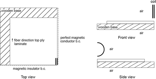
A magnetic insulator boundary condition was applied on the symmetry plane perpendicular to the coil windings. As a result, the magnetic field is zero in the normal direction, while current is only allowed to flow in normal direction. Mathematically, this is described as:

(10) $n\times A=0,$(10)

with A the magnetic potential, which is defined as:

(11) $\mathrm{\nabla }\times A=B$(11)

The other symmetry plane was implemented as a perfect magnetic conductor, which basically represent a mirror symmetry plane for the current:

(12) $n\times H=0.$(12)

All other boundaries were also considered magnetic conductors. However, as the outer 100 mm of airbox was meshed using infinite elements, which essentially apply a coordinate stretching to correctly represent the effect of the far-field boundary condition, the boundary condition here was found to not affect the solution.

The thermal model only comprised the laminate and the wooden base, while the surrounding air was represented by a convective boundary condition on all domain boundaries:

(13) $-{\lambda }_{\mathrm{n}}\frac{\mathrm{\partial }T}{\mathrm{\partial }n}=h\left(T-T_{\mathrm{\infty }}\right),$(13)

with the thermal conductivity along the unit normal on the surface, $h$ the heat transfer coefficient and the air temperature which set equal to room temperature. Perfect contact was assumed between the wooden base and laminate.

4.2.2. Material properties

The electric permittivity and magnetic permeability were obtained from the work by Lionetto et al. [20] and are listed in Table 2. Although these properties may depend on the microstructure, they are assumed similar for both material systems. Compared to the difference in electrical conductivity between the fiber and the matrix, which is at least 10 orders of magnitude, the differences in electrical permittivity and magnetic permeability between the matrix and the fiber are negligible [20]. Hence, compared to the electrical conductivity, the difference in permittivity and permeability between the two tapes is assumed to be negligible. The electric conductivities used in the model were presented in Section 3 and are listed in Table 1. The through-thickness value of the cross-ply laminates was used for the simulations as this incorporates the combined effect of the ply conductivity and the interface resistance. The thermal properties of the C/PEKK tape material were assumed independent of the manufacturer. Like the permittivity and permeability, this choice was based on the observation that the difference in thermal properties between the constituents is rather small. Figure 8 shows the thermal properties as a function of temperature, as used in this work. The left graph shows the density and specific heat, while the right graph shows the thermal conductivity both parallel and perpendicular to the fiber direction. The thermal properties of the C/PEKK tapes were assumed to be equal to those of a C/PEEK tape and were taken from Yousefpour and Hojjati [28]. The heat transfer coefficient h was chosen as 10 W/m²K.

Figure 8. Thermal material property data as used in the simulation in [28]. The left graph shows the density and specific heat as a function of temperature, while the right graph shows the thermal conductivity in fiber direction and perpendicular to the fiber direction, ${\lambda }_{\mathrm{z}}$

Table 2. Geometrical parameters, coil settings, material property data, and boundary condition values used for the simulations

Property	Symbol	Value
Solvay ply thickness	tply	0.137 mm
Toray ply thickness	tply	0.144 mm
Laminate surface area	Aply	290 × 290 mm^2
Wooden base thickness	twood	15 mm
Wooden base surface area	Awood	350 × 350 mm^2
Coil radius (center)	R	18.65 mm
Coil pitch	p	6.1 mm
Coil distance to laminate	δ	12.4 mm
Frequency	f	275 kHz
Coil current (RMS)	I	350 A
Absolute permittivity	ε0	8.85∙10^−12 F/m
Relative electric permittivity	ε r	3.7
Magnetic constant	μ0	4π∙10^−7 H/m
Relative magnetic permeability	μr	1
Heat transfer coefficient	h	10 W/m^2 K
Initial and room temperature	T∞	25°C
Wood thermal conductivity	λwood	0.21 W/m∙K
Wood specific heat	cp,wood	2180 J/kg∙K
Wood density	ρwood	817 kg/m^3

4.3. Simulations and data reduction

Two simulation models were implemented, one for each material. A Design of Experiments approach was then used to investigate the sensitivity of the model outcome to the electrical conductivities. A full factorial three-level three-factor design was chosen, resulting in 27 simulations for each material. The levels are indicated as low (−1), medium (0) and high (+1). For each factor, i.e. ${\sigma }_0$, ${\sigma }_{90}$ or ${\sigma }_{\mathrm{z}}$, the medium level was taken as the average of the measured electrical conductivity. The low and high values correspond to the average minus 5% and plus 5%, respectively. For sake of clarity, Table 3 lists the values used.

Table 3. Conductivity levels in S/m used in the sensitivity analysis

	Solvay			Toray
	Low	Medium	High	Low	Medium	High
${\sigma }_0$	2.18∙10^4	2.29∙10^4	2.40∙10^4	1.80∙10^4	1.89∙10^4	1.98∙10^4
${\sigma }_{90}$	3.20∙10°	3.37∙10°	3.54∙10°	8.39∙10°	8.83∙10°	9.27∙10°
${\sigma }_{\mathrm{z}}$	6.04∙10^−1	6.36∙10^−1	6.67∙10^−1	1.66∙10^−1	1.75∙10^−1	1.84∙10^−1

Table 4. Conductivity levels in S/m used in the material variability analysis

	Solvay			Toray
	Low	Medium	High	Low	Medium	High
${\sigma }_0$	2.24∙10^4	2.29∙10^4	2.34∙10^4	1.71∙10^4	1.89∙10^4	2.07∙10^4
${\sigma }_{90}$	3.31∙10°	3.37∙10°	3.43∙10°	8.55∙10°	8.83∙10°	9.11∙10°
${\sigma }_z$	3.25∙10^−1	6.36∙10^−1	9.47∙10^−1	1.48∙10^−1	1.75∙10^−1	2.02∙10^−1

Each simulation itself comprised of two parts. First, the electromagnetic problem was solved in the frequency domain, yielding the current distribution in the laminate. Subsequently, the transient thermal problem was solved in two steps. The first step concerned the heating phase and involved Joule heating, while the second step concerned the cooling phase and did not include the Joule heating. The heating times for each case were extracted from the experimental data and equalled 12.5 s for Solvay and 16.5 s for Toray.

After each simulation, the initial heating rate k on the top surface of the laminate directly under the coil was extracted as the slope in the time-temperature data at 75 °C. The initial heating rate is not affected too much by the thermal boundary conditions and thermal properties of the wooden base, minimizing the influence of errors in their estimation. The heating rates for the two materials were fitted on a linear regression model:

$k=\alpha +{\beta }_0{\chi }_0+{\beta }_{90}{\chi }_{90}+{\beta }_{\mathrm{z}}{\chi }_{\mathrm{z}}+{\beta }_{0,90}{\chi }_0{\chi }_{90}+{\beta }_{90,\mathrm{z}}{\chi }_{90}{\chi }_{\mathrm{z}}+{\beta }_{\mathrm{z},0}{\chi }_{\mathrm{z}}{\chi }_0+\text{isin},$

in which $\alpha$ is the average heating rate, ${\beta }_X$ represent the regression coefficients and $ϵ$ the error, which is minimized. The subscript of the variables ${\beta }_X$ and ${\chi }_X$ indicates to which conductivity it is related, while values for ${\chi }_X$ are taken as −1, 0 or +1 for low, medium or high, respectively.

5. Simulation results

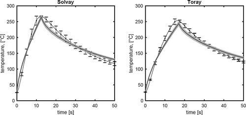
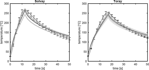
Figure 9 shows the simulation results combined with the experimentally obtained time vs. temperature curves. Although not obvious, each graph shows the data of the 27 simulations. The thick dark grey line corresponds to the center point of the DoE where the conductivities ${\sigma }_0$, ${\sigma }_{90}$ and ${\sigma }_{\mathrm{z}}$ are all equal to their average value, while the thin light grey lines show the data corresponding to the cases where at least one of the conductivities was equal to its low or high value. The lines corresponding to the simulation results are so close that they overlap, which suggests that a change of 5% for one or more factors has little effect on the simulation outcome. A decent overall agreement was found between the simulations and experiments. The heating rate is predicted well with an average measured and simulated heating rate of 29.9 °C/s and 30.4 °C/s, respectively, for the Solvay laminate, and 21.6 °C/s versus 19.4 °C/s for the Toray laminate.

Figure 9. Comparison of simulation and experimental results. The black line with the error bars represents the mean and standard deviation of the experimental data. The thick dark grey line gives simulation result using the mean values of the electrical conductivities, while the thin grey lines represent the simulation results in which one or more values of the electrical conductivity was varied with 5%

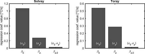
Figure 10 shows the regression coefficients for the statistically relevant factors for both laminates, while the full list of coefficients can be found in Table A1 in the appendix. The linear regression analysis showed that the heating rate at 75 °C is most sensitive to the electrical conductivity in fiber direction ${\sigma }_0$, moderately sensitive to the through-thickness conductivity ${\sigma }_{\mathrm{z}}$ and insensitive to the in-plane transverse conductivity ${\sigma }_{90}$. This observation corresponds to literature on the induction heating of UD reinforced laminates which state that, due to the low in-plane transverse conductivity, the current predominantly follows the fibers and relies on contact between the plies, thus effectively ${\sigma }_{\mathrm{z}}$, to change direction [11,14]. In addition to the main effects, a small interaction effect was observed for ${\sigma }_0$ and ${\sigma }_{\mathrm{z}}$. For sake of interpretation, a 5% increase in the electrical conductivity in fiber direction ${\sigma }_0$ results in an increase in heating rate of 3.5% and 2.8% for the Solvay and Toray laminate, respectively.

Figure 10. Relevant regression coefficients in Equation 1(1) $\mathrm{\nabla }\cdot E=\rho ,$(1) for the sensitivity analysis in which the electrical conductivity was varied by ±5%. The associated material property is indicated between brackets

6. Discussion

6.1. Electrical conductivity of C/PEKK

The electrical conductivity data presented in Table 1 showed differences between the two materials, even though both tapes are based on the same fiber and are based on a PEKK polymer. Although the fiber volume fractions for both materials are reported to be similar, the thickness data presented in Section 2.1 suggests otherwise. Based on the reported thicknesses, the fiber volume fraction is estimated as 60% for the Solvay laminates and 57% for the Toray laminates. However, since the in-plane conductivity of the Toray laminate exceeds the value for the Solvay laminate, the fiber volume fraction clearly is not the only relevant property. Therefore, surface and cross-sectional micrographs were made of the UD and cross-ply laminates in order to investigate whether the differences in conductivity can be related to the microstructure of the laminates.

The left and right image in Figure 11 show cross-sections of the Solvay and Toray cross-ply laminates, respectively. The fiber distribution in the plies of the Toray laminate is rather homogeneous compared to the distribution in the Solvay laminate, with the latter featuring clusters of fibers separated by resin rich regions. In fact, the cross-sectional micrographs of the laminates are quite like the cross-sections of the as-received tape materials shown in Figure 1. Arguably, the amount of fiber to fiber contacts is increased in the regions with clustered fibers, possibly providing a conductive path through the thickness of the cross-ply laminate and thereby explaining the higher through-thickness of conductivity of the Solvay laminate.

Figure 11. Cross-sectional micrographs of the Solvay (left) and Toray (right) cross-ply laminates

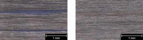
Figure 12 shows surface micrographs of the UD laminates. Like the as-received tape and the cross-ply laminate, resin rich regions can be observed between clusters of closely packed fibers from the surface micrograph of the Solvay laminate. Conversely, the surface micrograph of the Toray laminate is more homogeneous and presumably lacks resin rich regions between the fibers. The presence of the resin regions may inhibit the current in the in-plane transverse direction and thereby explain that the Solvay material has a lower in-plane transverse conductivity compared to the Toray material. The difference in the electrical conductivity in fiber direction between the two materials cannot readily be explained from the micrographs and requires further study. The relation between microstructure, which not only depends on the materials used but also on the processing history, and the electrical conductivities seems of such importance that it is worthy a dedicated study in itself.

Figure 12. Surface micrographs a Solvay (left) and Toray (right) UD laminates.6.2 Effect of material variability

6.2. Effect of material variability

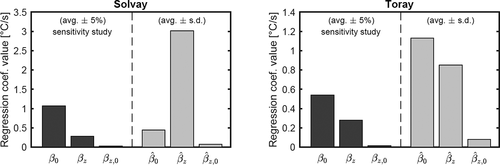
The regression coefficients plotted in Figure 10 illustrated that the simulation results are most sensitive to variations in the conductivity in fiber direction ${\sigma }_0$ and in the through-thickness direction ${\sigma }_{\mathrm{z}}$. These results reinforce the idea that the eddy currents primarily follow the fibers and rely on the through-thickness conductivity to move to neighboring plies with a different orientation. Although the sensitivity study provides useful insights in the physics governing the process, it does not provide a confidence interval for the simulation results as this is determined by, among other, the variability in the material property data or boundary conditions. Some of the experimentally determined conductivities, as presented in Table 1, showed a large variability. A similar Design of Experiments approach was followed to investigate how this variability in the measured conductivities affects the heating of the laminates. The factors are in this case not varied by 5% as was done for the sensitivity analysis, but with their standard deviation in the experimental results as listed in Table 1. Thus, as before, the medium level for each factor was taken as the average of the electrical conductivity, but now the low and high values correspond to the average minus one standard deviation and the average plus one standard deviation. Table 4 lists the used levels for sake of completeness.

Again, heating rate at 75°C was fitted on a linear regression model:

$k=\hat{\alpha }+{\hat{\beta }}_0{\chi }_0+{\hat{\beta }}_{90}{\chi }_{90}+{\hat{\beta }}_{\mathrm{z}}{\chi }_{\mathrm{z}}+{\hat{\beta }}_{0,90}{\chi }_0{\chi }_{90}+{\hat{\beta }}_{90,\mathrm{z}}{\chi }_{90}{\chi }_{\mathrm{z}}+{\hat{\beta }}_{\mathrm{z},0}{\chi }_{\mathrm{z}}{\chi }_0+\text{isin},$

in which the hat above the coefficients now indicates that these belongs to the DoE which analyzed the effect of material variability.

Figure 13 compares the simulation results to the experimental data. As in Figure 9, each graph shows the data of 27 simulations, with the thick dark grey line corresponding to the center point of the DoE. Here also, some of the simulation results are so close that they overlap which suggests that the variability of one or more factors have a negligible effect on the simulation outcome. Although overall the agreement between model and experiment seems acceptable, the graphs do illustrate that the variability in the electrical conductivity can have a significant effect on the temperature evolution. For example, a difference in maximum temperature of more than 30 °C was found for the Solvay laminate, which, in the context of welding processes, can be the difference between a successful and a failing joint. The graphs also illustrate that the experimentally observed variation in the temperature evolution is of the same order of magnitude as the simulated effect of variability in the conductivity. It is, however, difficult to directly and unequivocally correlate the variability in conductivity with the measured temperature, as the measured temperature data is subject to other sources of error, such as e.g. varying (thermal) boundary conditions, possible inaccuracies in coil positioning and operator influences.

Figure 13. Comparison of simulation and experimental results. The black line with the error bars represents the mean and standard deviation of the experimental data, the thick dark grey line gives simulation result using the mean values of the electrical conductivities, while the thin grey lines represent the simulation results in which one or more values of the electrical conductivity was varied with one standard deviation

Table A2 lists the regression coefficients ${\hat{\beta }}_X$, while the significant coefficients are plotted in Figure 14 alongside the coefficients obtained from the sensitivity analysis. The left graph shows that the variability in through-thickness conductivity ${\sigma }_{\mathrm{z}}$ has the largest effect on the heating rate for the Solvay laminate, which is not surprising given a coefficient of variation in the experimental data of 48%. For reference, a value for ${\hat{\beta }}_{\mathrm{z}}$ of 3 °C/s corresponds to a change in heating rate of 10% for the Solvay laminate. The variability in the conductivity in fiber direction ${\sigma }_0$ has a small influence on the heating rate, while the effect of the transverse in-plane conductivity ${\sigma }_{90}$ was found to be negligible. The right graph in Figure 14 shows the significant regression coefficients for the Toray laminate. Here, the heating rate is mostly affected by the variability in the conductivity in fiber direction ${\sigma }_0$ and in the through-thickness direction ${\sigma }_{\mathrm{z}}$. For reference, the coefficient of variation of ${\sigma }_0$ and ${\sigma }_{\mathrm{z}}$ for the Toray material was 10% and 15%, respectively. The simulation results presented here show that the variability in material properties can have a large influence on the heating behavior.

Figure 14. Comparison of the relevant regression coefficients for the sensitivity analysis (avg. ± 5%) and the material variability study (avg. ± s.d.)

7. Conclusions and recommendations

The anisotropic electrical conductivities of commercially available Solvay and Toray C/PEKK tape materials were determined experimentally at room temperature. Although the measured conductivities were of the same order of magnitude, small differences were observed between the two materials. Most notably, the Solvay laminates had a higher through-thickness conductivity, but a lower transverse in-plane conductivity than the Toray laminates. Surface and cross-section microscopy images showed that the two tapes differ significantly in morphology. The Solvay tape and laminates feature an inhomogeneous fiber distribution, with resin rich regions, almost over the full ply thickness, between clusters of fibers. Conversely, the Toray tape and laminates showed a homogeneous fiber distribution. Arguably, the resin rich regions reduce the in-plane transverse conductivity, while the fiber clusters facilitate fiber to fiber contact thereby increasing the through-thickness conductivity.

A simulation model was implemented for the induction heating of UD tape-based thermoplastic composites. The simulation model was validated experimentally and showed good agreement with heating experiments performed on cross-ply laminates. The influence of the variability in the experimentally determined electrical conductivities was studied using the simulation model. It was shown that the variability in the electrical conductivities can have a significant effect on the temperature evolution. Therefore, robust induction heating and welding requires optimization techniques that account for this variability, for which the model presented in this work could form the basis.

Acknowledgements

The authors gratefully acknowledge the financial and technical support from the industrial and academic members of the ThermoPlastic composites Research Center (TPRC), as well as the support funding from the Province of Overijssel for improving the regional knowledge position within the Technology Base Twente initiative.

Disclosure statement

No potential conflict of interest was reported by the authors.

Appendices

Table A1. Results from the linear regression analysis for the sensitivity study in which the factors were varied with ± 5%

	Solvay		Toray
	Regression coef. value [°C/s]	p-value	Regression coef. value [°C/s]	p-value
$\hat{\alpha }$ (avg.)	30.37	< 0.01	19.39	< 0.01
${\beta }_0$	1.07	< 0.01	5.40∙10^−1	< 0.01
${\beta }_{90}$	4.75∙10^−4	0.90	1.94∙10^−3	0.88
${\beta }_z$	2.80∙10^−1	< 0.01	2.78∙10^−1	< 0.01
${\beta }_{0,90}$	-2.30∙10^−6	1.0	2.27∙10^−5	1.0
${\beta }_{90,z}$	-7.28∙10^−6	1.0	-3.21∙10^−5	1.0
${\beta }_{z,0}$	2.90∙10^−2	< 0.01	1.43∙10^−2	0.36

Table A2. Results from the linear regression analysis for the material variability study in which the factors were varied with the ± standard deviation

	Solvay		Toray
	Regression coef. value [°C/s]	p-value	Regression coef. value [°C/s]	p-value
$\alpha$ (avg.)	29.7	< 0.01	19.34	< 0.01
${\hat{\beta }}_0$	4.44∙10^−1	< 0.01	1.13	< 0.01
${\hat{\beta }}_{90}$	1.77∙10^−4	1.0	1.23∙10^−3	0.93
${\hat{\beta }}_z$	3.02	< 0.01	8.51∙10^−1	< 0.01
${\hat{\beta }}_{0,90}$	6.83∙10^−7	1.0	2.04∙10^−5	1.0
${\hat{\beta }}_{90,z}$	-3.10∙10^−5	1.0	-6.19∙10^−5	1.0
${\hat{\beta }}_{z,0}$	6.90∙10^−2	0.65	7.94∙10^−2	< 0.01

References

- Thermoplastic fuselage demonstrator [ Online]. [cited 2019 Apr 10]. Available from: http://www.jeccomposites.com/knowledge/international-composites-news/thermoplastic-fuselage-demonstrator
- Gardiner G. Thermoplastic composite demonstrators — EU roadmap for future airframes. Compos World [ Online]. [cited 28 May 2018]. Available from: https://www.compositesworld.com/articles/thermoplastic-composite-demonstrators-eu-roadmap-for-future-airframes-
- Ishii K, Todoroki A, Mizutani Y, et al. Bending fracture rule for 3D-printed curved continuous-fiber composite. Adv Compos Mater. 2019;28(4):383–395.
- Shiratori H, Todoroki A, Ueda M, et al. Mechanism of folding a fiber bundle in the curved section of 3D printed carbon fiber reinforced plastics. Adv Compos Mater. 2020;29(3):247–257.
- Todoroki A, Oasada T, Mizutani Y, et al. Tensile property evaluations of 3D printed continuous carbon fiber reinforced thermoplastic composites. Adv Compos Mater. 2020;29(2):147–162.
- Ageorges C, Ye L, Hou M. Advances in fusion bonding techniques for joining thermoplastic thermoplastic matrix composites: a review. Compos Part A. 2001;32:839–857.
- Yousefpour A, Hojjati M, Immarigeon J-P. Fusion bonding/welding of thermoplastic composites. J Thermoplast Composite Mater. 2004;17:303–340.
- Ahmed T, Stavrov D, Bersee H, et al. Induction welding of thermoplastic composites - an overview. Compos Part A. 2006;37(10):1638–1651.
- Bayerl T, Duhovic M, Mitschang P, et al. The heating of polymer composties by electromagnetic induction - a review. Compos Part A. 2014;37(10):27–40.
- Choudhury M, Debnath D. A review of the research and advances in electromagnetic joining of fiber-reinforced thermoplastic composites. Polym Eng Sci. 2019;59(10):1965–1985. In press.
- Kim H, Yarlagadda S, Gillespie J, et al. A study on the induction heating of carbon fiber reinforced thermoplastic composites. Adv Compos Mater. 2002;11(1):71–80.
- Yarlagadda S, Kim H, Gillespie J, et al. A study on the induction heating of conductive fiber reinforced composites. J Compos Mater. 2002;36(4):401–421.
- Rudolf R, Mitschang P, Neitzel M. Induction heating of continuous carbon-fiber-reinforced thermoplastics. Compos Part A. 2000;31(11):1191–1202.
- Xu X, Ji H, Cheng J, et al. Inerlaminar contact resistivity and its influence on eddy currents in carbon fiber reinforced polymer laminates. NDT E Int. 2018;94:79–91.
- Wasselynk G, Trichet D, Ramdane B, et al. Microscopic and macroscopic electromagnetic and thermal modeling of carbon fier reinfoced polymer composites. IEEE Trans Magn. 2011;47(5):1114–1117.
- Van Ingen J, Buitenhuis A, Van Wijngaarden M, et al. Development of the Gulfstream G650 induction welded thermoplastic elevators and rudder. International SAMPE symposium and exhibition; Seattle (WA); 2010.
- Taketa I, Kalinka G, Gorbatick L, et al. Influence of cooling rate on the properties of carbon fiber unidirectional composites with polypropylene, polyamide 6, and polyphenylene sulfide matrices. Adv Compos Mater. 2020;29(1):101–113.
- Duhovic M, Moser L, Mitschang P, et al. Simulation of the joining of composite materials by electromagnetic induction. 12th international LS-DYNA user conference; 2012.
- Pappada S, Salomi A, Montanaro J, et al. Fabrication of a thermoplastic matrix composite stiffened panel by induction welding. Aerosp Sci Technol. 2015;43:314–320.
- Lionetto F, Pappada S, Buccoliero G, et al. Finite element modeling of continuous induction welding of thermoplastic matrix composites. Mater Des. 2017;120:212–221.
- Duhovic M, Hümbert M, Mitschang P, et al. Further advances in simulating the processing of composite materials by electromagnetic induction. 13th international LS-DYNA user conference; Detroit, MI, United States of America. 2014.
- Bensaid S, Trichet D, Fouladgar J. 3-D simulation of induction heating of anisotropic composite materials. IEEE Trans Magn. 2005;41(5):1568–1571.
- Bensaid S, Trichet D, Fouladgar J. Electromagnetic and thermal behaviors of multilayer anisotropic composite materials. IEEE Trans Magn. 2006;42(4):995–998.
- O’Saughnessey P, Dube M, Villegas I. Modeling and experimental investigation of induction welding of thermoplastic composites and comparison with other welding processes. J Compos Mater. 2015;50(1):2895–2910.
- Singh Y, “Electrical resistivity measurements: a review. Int J Mod Phy Conf Ser. 2013;22:745–756.
- Sheet HPD. HexTow(R) AS4 carbon fiber.Material Data Sheet.
- Quiroga Cortès L, Racagel S, Lonjon A, et al. Electrically conductive carbon fiber/PEKK/silver nanowires multifunctional composites. Compos Sci Technol. 2016;137:159–166.
- Yousefpour A, Hojjati M. Welding thermoplastics and thermoplastic composite materials. Chichester (UK): John Wiley & Sons; 2011.