The quantum theory of the Penning trap

Abstract

We present the quantum theory of the Penning trap in terms of individual x and y radial modes of the motion of a single charged particle in the trap, and demonstrate how the conventional rotating frame used to examine these individual dynamics fails in the quantum regime. In solving the radial Hamiltonian in the $\{x,y\}$ basis, we show how canonical transformation of the variables must take place after quantization, in order that these separate motions can be consistently tracked. This is in contrast to previous work. The results of the discussion lend themselves to a fully quantum treatment of mode coupling in the trap, leading to an avoided crossing between the coupled energy levels of the system. Exploiting the algebraic structure of the problem allows employment of a dressed-atom formalism within quantum Penning trap theory, and future applications resulting from this are proposed.

Keywords:

• Penning trap theory
• quantum mode coupling
• dressed-atom formalism
• trapped electrons

1. Introduction

The fundamental theory of the Penning trap has been studied extensively and successfully [1–4], laying down the framework of a device responsible for the most precise value of the g-factor [5] and mass [6] of the electron, with far reaching and ever expanding applications [7–10]. The power of this particular ion trap must surely lie in its inherent simplicity; the static electric and magnetic fields used for confinement produce a Hamiltonian which is exactly solvable by a number of methods [2].

This paper is motivated by the pursuit of quantum information processing by confinement of single electrons in Penning traps [8,11–14]. Electrons are highly suitable candidates for the implementation of quantum logic [15], and the use of Penning traps for their confinement further takes advantage of the high precision of measurement enabled in this trap [16], and the well-controlled decoherence effects it offers [1]. Furthermore, the implementation of the Penning trap as a quantum radar through quantum illumination protocols [17–22] is a possibility enabled by the unique design of the Geonium Chip trap [10,23,24], which can only follow from a consistent quantum theory. A further motivation of this work is the possibility of quantum interferometry through the manipulation of the adiabatic potential in the trap [25], for which knowledge of the x and y motions in the quantum regime is essential.

The principal method of diagonalizing the classical $\{x,y\}$ basis before quantization of canonical variables [4] and treating the quantized radial motion in terms of cyclotron $(+)$ and magnetron $(-)$ modes is the most well-established. This method lends itself well to the description of the radial dynamics as that of a two-dimensional isotropic oscillator rotating around the z-axis [2], forming an epicyclic curve in the x, y plane. In this paper, we discuss how combining the separate x and y motions in this way, before quantization, disguises the nature of these individual motions in the quantum regime, and leads to a misguided interpretation of the potential energy in the system. We hold the non-conservative force contributed by the magnetic field responsible, and propose an alternative approach to the quantum treatment when knowledge of individual spatial modes is desirable. This motivates the use of sets of Schwinger boson angular momentum algebra within the Penning trap [26]. Such methods have been employed in Penning trap theory in [27], but in the present work they are used to enable a fully quantum treatment of the Penning trap in the dressed-atom formalism [28,29].

The paper is divided into six main sections. In Section 2, we review the classical Penning trap Hamiltonian, and the transformation to a frame rotating around the z-axis. Section 3 examines the quantum Hamiltonian and transformation to this frame in the $\{x,y\}$ basis, anddiscusses how this approach fails when interpreting individual x and y dynamics for low energy states. Section 4 then presents a novel approach in solving the quantum theory of the Penning trap, and discusses the advantage of this formulation over the conventional approach [1–4]. Section 5 examines how the devised methods can be employed in a quantum mode coupling calculation, and proposes some future applications which exploit the results of the calculation. We summarize the outcomes and their future implications in Section 6.

2. The classical theory of the Penning trap

2.1. The Hamiltonian

Confinement of charged particles in a Penning trap is provided a static electric field $\overrightarrow{E}=-\overrightarrow{\mathrm{\nabla }}\mathit{\varphi }(\overrightarrow{r})$ and axial magnetic field $\overrightarrow{B}=|\overrightarrow{B}|{\widehat{e}}_z$. In an ideal circular Penning trap, the associated electric potential of the former provides the quadrupole(1) $$\begin{array}{c}\hfill \mathit{\varphi }(\overrightarrow{r})=U_0\left(z^2-\frac{x^2+y^2}{2}\right),\end{array}$$(1)

where the units of $U_0$ are $\mathrm{V}{m}^{-2}$, and the sign of this field curvature depends upon the charge of the trapped particle(s). Beginning with the Lagrangian for a (positively) charged particle of mass m and charge q in the presence of static electric and magnetic fields with associated potentials $\mathit{\varphi }(\overrightarrow{r}),$$\overrightarrow{A}(\overrightarrow{r})$:(2) $$\begin{array}{c}\hfill \mathcal{L}=\frac{1}{2}m{\overrightarrow{v}}^2-q\mathit{\varphi }(\overrightarrow{r})+q\overrightarrow{v}·\overrightarrow{A}(\overrightarrow{r}).\end{array}$$(2)

We find the form of the conjugate momenta, $p_i=\frac{\mathit{\delta }\mathcal{L}}{\mathit{\delta }{v}_i}=m{v}_i+q{A}_i,$ and the subsequent Hamiltonian:(3) $$\begin{array}{cc}\hfill \mathcal{H}& =\overrightarrow{v}·\overrightarrow{p}-\mathcal{L}\hfill \\ \hfill & =\frac{1}{2m}{(\overrightarrow{p}-q\overrightarrow{A}(\overrightarrow{r}))}^2+q\mathit{\varphi }(\overrightarrow{r}).\hfill \end{array}$$(3)

In the Coulomb gauge $\overrightarrow{\mathrm{\nabla }}·\overrightarrow{A}(\overrightarrow{r})=0$ [30] the convenient vector potential $\overrightarrow{A}(\overrightarrow{r})=\frac{1}{2}\overrightarrow{B}\times \overrightarrow{r}$ is chosen [1] to produce the components(4) $$\begin{array}{c}\hfill A_x=-\frac{1}{2}By,A_y=\frac{1}{2}Bx,A_z=0.\end{array}$$(4)

In this paper, the trapping of a single electron is considered, and inserting (4(4) $$\begin{array}{c}\hfill A_x=-\frac{1}{2}By,A_y=\frac{1}{2}Bx,A_z=0.\end{array}$$(4) ) into (3(3) $$\begin{array}{cc}\hfill \mathcal{H}& =\overrightarrow{v}·\overrightarrow{p}-\mathcal{L}\hfill \\ \hfill & =\frac{1}{2m}{(\overrightarrow{p}-q\overrightarrow{A}(\overrightarrow{r}))}^2+q\mathit{\varphi }(\overrightarrow{r}).\hfill \end{array}$$(3) ), the classical Hamiltonian of the electron of charge $q=-e$ in this ideal configuration is given by(5) $$\begin{array}{cc}\hfill \mathcal{H}& =\frac{1}{2m}\left(p_x^2+p_y^2+p_z^2\right)+\frac{{\mathit{\omega }}_c}{2}(x{p}_y-y{p}_x)\hfill \\ \hfill & +\frac{1}{2}m{\left(\frac{{\mathit{\omega }}_1}{2}\right)}^2(x^2+y^2)+\frac{1}{2}m{\mathit{\omega }}_z^2{z}^2,\hfill \end{array}$$(5) where(6) $$\begin{array}{c}\hfill {\mathit{\omega }}_c=\frac{|q||\overrightarrow{B}|}{m},{\mathit{\omega }}_z=\sqrt{\frac{2q{U}_0}{m}},{\mathit{\omega }}_1=\sqrt{{\mathit{\omega }}_c^2-2{\mathit{\omega }}_z^2}.\end{array}$$(6)

The motion in the radial plane is now conventionally decoupled by canonical transformation [2], and the Hamiltonian is written in terms of three distinct harmonic contributions: the cyclotron ($+$), axial (z), and magnetron ($-$) motions. As a consequence of the crossing of the electric and magnetic fields, the magnetron motion is unstable, and must therefore be minimized to prevent the electron striking the edge of the trap [31]. The frequencies of the radial modes are given explicitly by(7) $$\begin{array}{c}\hfill {\mathit{\omega }}_{+}=\frac{1}{2}\left({\mathit{\omega }}_c+{\mathit{\omega }}_1\right),{\mathit{\omega }}_{-}=\frac{1}{2}\left({\mathit{\omega }}_c-{\mathit{\omega }}_1\right).\end{array}$$(7)

Figure 1. The classical radial motion of a charged particle in the circular Penning trap traces out an epicyclic curve [1] in the x-y plane. The cyclotron motion of frequency ${\mathit{\omega }}_{+}$ is superposed onto a slow magnetron drift orbit with frequency ${\mathit{\omega }}_{-}$. The relative size of the orbits is not drawn to scale.

We identify $x{p}_y-y{p}_x$ in (5(5) $$\begin{array}{cc}\hfill \mathcal{H}& =\frac{1}{2m}\left(p_x^2+p_y^2+p_z^2\right)+\frac{{\mathit{\omega }}_c}{2}(x{p}_y-y{p}_x)\hfill \\ \hfill & +\frac{1}{2}m{\left(\frac{{\mathit{\omega }}_1}{2}\right)}^2(x^2+y^2)+\frac{1}{2}m{\mathit{\omega }}_z^2{z}^2,\hfill \end{array}$$(5) ) with the z component of canonical angular momentum, so that the radial part of the classical Hamiltonian is that of a cranked harmonic oscillator [32], a two-dimensional harmonic oscillator with an additional rotation of the plane around the z-axis at the frequency ${\mathit{\omega }}_c/2$. The harmonic motion of the x and y components in the Hamiltonian are at the same frequency ${\mathit{\omega }}_1/2$. The epicyclic curve traced by the classical expectation values [1] comprises a fast (typically $\sim$GHz) cyclotron orbit superposed upon a slow magnetron drift ($\sim$kHz), as shown in Figure 1. This motion is then superposed upon simple harmonic oscillation along the z-axis.

Crucially, the harmonic frequency of the $x,y$ oscillators, ${\mathit{\omega }}_1/2$, does not match the cranking frequency, ${\mathit{\omega }}_c/2$ in (5(5) $$\begin{array}{cc}\hfill \mathcal{H}& =\frac{1}{2m}\left(p_x^2+p_y^2+p_z^2\right)+\frac{{\mathit{\omega }}_c}{2}(x{p}_y-y{p}_x)\hfill \\ \hfill & +\frac{1}{2}m{\left(\frac{{\mathit{\omega }}_1}{2}\right)}^2(x^2+y^2)+\frac{1}{2}m{\mathit{\omega }}_z^2{z}^2,\hfill \end{array}$$(5) ). This arises from the necessity of providing axial confinement in the trap: the Laplace equation dictates that we cannot provide a static potential minimum along the z-axis alone [30], and a fraction of the axial trapping frequency must be added to the radial one. As a result ${\mathit{\omega }}_c\to {\mathit{\omega }}_1$, and the Landau levels [33] of the magnetic field become non-degenerate. This has significant consequences for the expectation values of the quantum system, further discussed in Section 3.3.

2.2. The classical rotating frame

An operation which greatly simplifies Hamiltonian (5(5) $$\begin{array}{cc}\hfill \mathcal{H}& =\frac{1}{2m}\left(p_x^2+p_y^2+p_z^2\right)+\frac{{\mathit{\omega }}_c}{2}(x{p}_y-y{p}_x)\hfill \\ \hfill & +\frac{1}{2}m{\left(\frac{{\mathit{\omega }}_1}{2}\right)}^2(x^2+y^2)+\frac{1}{2}m{\mathit{\omega }}_z^2{z}^2,\hfill \end{array}$$(5) ) is the time-dependent transformation to the frame rotating around the z-axis [2]. We begin by defining the change of coordinates of the system:(8) $$\begin{array}{cc}& x\to xcos\mathrm{\Omega }t-ysin\mathrm{\Omega }t,\hfill \\ \hfill & y\to xsin\mathrm{\Omega }t+ycos\mathrm{\Omega }t.\hfill \end{array}$$(8)

This describes rotation around the z-axis at frequency $\mathrm{\Omega }$, in the same anticlockwise direction as the rotation caused by the force on the electron in the magnetic field. In this frame, the Hamiltonian becomes(9) $$\begin{array}{cc}\hfill \mathcal{H}& \to \frac{1}{2m}\left(p_x^2+p_y^2+p_z^2\right)+\left(\frac{1}{2}{\mathit{\omega }}_c-\mathrm{\Omega }\right)(x{p}_y-y{p}_x)\hfill \\ \hfill & +\frac{m}{2}{\left(\frac{{\mathit{\omega }}_1}{2}\right)}^2(x^2+y^2)+\frac{1}{2}m{\mathit{\omega }}_z^2{z}^2,\hfill \end{array}$$(9)

and the canonical momenta of the radial motion:(10) $$\begin{array}{cc}& p_x\to m\dot{x}+my\left(\frac{1}{2}{\mathit{\omega }}_c-\mathrm{\Omega }\right),\hfill \\ \hfill & p_y\to m\dot{y}-mx\left(\frac{1}{2}{\mathit{\omega }}_c-\mathrm{\Omega }\right).\hfill \end{array}$$(10)

By a judicious choice of $\mathrm{\Omega }={\mathit{\omega }}_c/2$, the angular momentum term is removed from the Hamiltonian:(11) $$\begin{array}{cc}\hfill \mathcal{H}\stackrel{\mathrm{\Omega }={\mathit{\omega }}_c/2}{⟶}{\mathcal{H}}_{\mathrm{\Omega }}& =\frac{1}{2m}(p_x^2+p_y^2+p_z^2)\hfill \\ \hfill & +\frac{m}{2}{\left(\frac{{\mathit{\omega }}_1}{2}\right)}^2(x^2+y^2)+\frac{1}{2}m{\mathit{\omega }}_z^2{z}^2,\hfill \end{array}$$(11)

and from (10(10) $$\begin{array}{cc}& p_x\to m\dot{x}+my\left(\frac{1}{2}{\mathit{\omega }}_c-\mathrm{\Omega }\right),\hfill \\ \hfill & p_y\to m\dot{y}-mx\left(\frac{1}{2}{\mathit{\omega }}_c-\mathrm{\Omega }\right).\hfill \end{array}$$(10) ), the canonical momenta likewise reduce to a purely kinetic form [2]. Thus the rotating frame Hamiltonian (11(11) $$\begin{array}{cc}\hfill \mathcal{H}\stackrel{\mathrm{\Omega }={\mathit{\omega }}_c/2}{⟶}{\mathcal{H}}_{\mathrm{\Omega }}& =\frac{1}{2m}(p_x^2+p_y^2+p_z^2)\hfill \\ \hfill & +\frac{m}{2}{\left(\frac{{\mathit{\omega }}_1}{2}\right)}^2(x^2+y^2)+\frac{1}{2}m{\mathit{\omega }}_z^2{z}^2,\hfill \end{array}$$(11) ) reveals an isotropic oscillator in the radial plane, along with the original axial motion. In Section 3.3, the calculation is repeated for a quantized system in an $\{x,y\}$ radial basis, revealing surprising inconsistencies in the expectation values of the system resulting from this treatment.

Other interesting choices of the frequency $\mathrm{\Omega }$ are the slow magnetron drift ${\mathit{\omega }}_{-}$ and the reduced cyclotron frequency ${\mathit{\omega }}_{+}$ [2]. Plugging the former into (9(9) $$\begin{array}{cc}\hfill \mathcal{H}& \to \frac{1}{2m}\left(p_x^2+p_y^2+p_z^2\right)+\left(\frac{1}{2}{\mathit{\omega }}_c-\mathrm{\Omega }\right)(x{p}_y-y{p}_x)\hfill \\ \hfill & +\frac{m}{2}{\left(\frac{{\mathit{\omega }}_1}{2}\right)}^2(x^2+y^2)+\frac{1}{2}m{\mathit{\omega }}_z^2{z}^2,\hfill \end{array}$$(9) ):(12) $$\begin{array}{cc}\hfill \mathcal{H}\stackrel{\mathrm{\Omega }={\mathit{\omega }}_{-}}{\to }{\mathcal{H}}_{{\mathit{\omega }}_{-}}& =\frac{1}{2m}\left(p_x^2+p_y^2+p_z^2\right)\hfill \\ \hfill & +\frac{m}{2}{\left(\frac{{\mathit{\omega }}_1}{2}\right)}^2\left(x^2+y^2\right)\hfill \\ \hfill & +\frac{{\mathit{\omega }}_1}{2}\left(x{p}_y-y{p}_x\right)+\frac{1}{2}m{\mathit{\omega }}_z^2{z}^2.\hfill \end{array}$$(12)

The radial part of this Hamiltonian is identical to that of an electron in a magnetic field with Larmor frequency ${\mathit{\omega }}_1/2$ [33]; the rotating frame at this frequency appears to remove any effects of the electric field. The choice $\mathrm{\Omega }={\mathit{\omega }}_{+}$ similarly reduces the radial part of $\mathcal{H}$ to the Landau Hamiltonian with the opposite sign of angular momentum:(13) $$\begin{array}{cc}\hfill \mathcal{H}\stackrel{\mathrm{\Omega }={\mathit{\omega }}_{+}}{\to }{\mathcal{H}}_{{\mathit{\omega }}_{+}}& =\frac{1}{2m}\left(p_x^2+p_y^2+p_z^2\right)\hfill \\ \hfill & +\frac{m}{2}{\left(\frac{{\mathit{\omega }}_1}{2}\right)}^2\left(x^2+y^2\right)\hfill \\ \hfill & -\frac{{\mathit{\omega }}_1}{2}\left(x{p}_y-y{p}_x\right)+\frac{1}{2}m{\mathit{\omega }}_z^2{z}^2.\hfill \end{array}$$(13)

This is the effective Hamiltonian of a positron particle in a magnetic field with Larmor frequency ${\mathit{\omega }}_1/2$ [2].

Our interest in this paper is on the separate dynamics of the x and y motions, so we will focus on the choice of frequency $\mathrm{\Omega }={\mathit{\omega }}_c/2$ which effectively decouples them.

3. Rotating frame approach

3.1. The quantum Hamiltonian

Imposing the canonical commutation relations $[{\widehat{q}}_i,{\widehat{p}}_j]=iħ{\mathit{\delta }}_{\mathit{ij}}$ upon canonically conjugate classical variables $q_i$ and $p_j$ allows construction of a set of quantum creation and annihilation operators. In the present work, their form is determined by the straightforward approach of writing the quantized version of the classical Hamiltonian (5(5) $$\begin{array}{cc}\hfill \mathcal{H}& =\frac{1}{2m}\left(p_x^2+p_y^2+p_z^2\right)+\frac{{\mathit{\omega }}_c}{2}(x{p}_y-y{p}_x)\hfill \\ \hfill & +\frac{1}{2}m{\left(\frac{{\mathit{\omega }}_1}{2}\right)}^2(x^2+y^2)+\frac{1}{2}m{\mathit{\omega }}_z^2{z}^2,\hfill \end{array}$$(5) ) in terms of individual x, y and z degrees of freedom:(14) $$\begin{array}{cc}\hfill {\widehat{a}}_x& =\frac{1}{\sqrt{2ħ}}\left(\sqrt{\frac{m{\mathit{\omega }}_1}{2}}\widehat{x}+i\sqrt{\frac{2}{m{\mathit{\omega }}_1}}{\widehat{p}}_x\right),\hfill \\ \hfill {\widehat{a}}_x^{†}& =\frac{1}{\sqrt{2ħ}}\left(\sqrt{\frac{m{\mathit{\omega }}_1}{2}}\widehat{x}-i\sqrt{\frac{2}{m{\mathit{\omega }}_1}}{\widehat{p}}_x\right),\hfill \end{array}$$(14) (15) $$\begin{array}{cc}\hfill {\widehat{a}}_y& =\frac{1}{\sqrt{2ħ}}\left(\sqrt{\frac{m{\mathit{\omega }}_1}{2}}\widehat{y}+i\sqrt{\frac{2}{m{\mathit{\omega }}_1}}{\widehat{p}}_y\right),\hfill \\ \hfill {\widehat{a}}_y^{†}& =\frac{1}{\sqrt{2ħ}}\left(\sqrt{\frac{m{\mathit{\omega }}_1}{2}}\widehat{y}-i\sqrt{\frac{2}{m{\mathit{\omega }}_1}}{\widehat{p}}_y\right),\hfill \end{array}$$(15) (16) $$\begin{array}{cc}\hfill {\widehat{a}}_z& =\frac{1}{\sqrt{2ħ}}\left(\sqrt{m{\mathit{\omega }}_z}\widehat{z}+i\frac{1}{\sqrt{m{\mathit{\omega }}_z}}{\widehat{p}}_z\right),\hfill \\ \hfill {\widehat{a}}_z^{†}& =\frac{1}{\sqrt{2ħ}}\left(\sqrt{m{\mathit{\omega }}_z}\widehat{z}-i\frac{1}{\sqrt{m{\mathit{\omega }}_z}}{\widehat{p}}_z\right).\hfill \end{array}$$(16) These obey the appropriate commutation relations $[{\widehat{a}}_x,{\widehat{a}}_x^{†}]=[{\widehat{a}}_y,{\widehat{a}}_y^{†}]=[{\widehat{a}}_z,{\widehat{a}}_z^{†}]=1$, with all other commutators going to zero, and enable us to write the quantized Hamiltonian:(17) $$\begin{array}{cc}\hfill \widehat{\mathcal{H}}& =ħ\frac{{\mathit{\omega }}_1}{2}\left({\widehat{a}}_x^{†}{\widehat{a}}_x+\frac{1}{2}\right)+ħ\frac{{\mathit{\omega }}_1}{2}\left({\widehat{a}}_y^{†}{\widehat{a}}_y+\frac{1}{2}\right)\hfill \\ \hfill & -iħ\frac{{\mathit{\omega }}_c}{2}\left({\widehat{a}}_x^{†}{\widehat{a}}_y-{\widehat{a}}_y^{†}{\widehat{a}}_x\right)+ħ{\mathit{\omega }}_z\left({\widehat{a}}_z^{†}{\widehat{a}}_z+\frac{1}{2}\right).\hfill \end{array}$$(17)

Throughout this paper, we will primarily use the notation of Equations (14(14) $$\begin{array}{cc}\hfill {\widehat{a}}_x& =\frac{1}{\sqrt{2ħ}}\left(\sqrt{\frac{m{\mathit{\omega }}_1}{2}}\widehat{x}+i\sqrt{\frac{2}{m{\mathit{\omega }}_1}}{\widehat{p}}_x\right),\hfill \\ \hfill {\widehat{a}}_x^{†}& =\frac{1}{\sqrt{2ħ}}\left(\sqrt{\frac{m{\mathit{\omega }}_1}{2}}\widehat{x}-i\sqrt{\frac{2}{m{\mathit{\omega }}_1}}{\widehat{p}}_x\right),\hfill \end{array}$$(14) )–(17(17) $$\begin{array}{cc}\hfill \widehat{\mathcal{H}}& =ħ\frac{{\mathit{\omega }}_1}{2}\left({\widehat{a}}_x^{†}{\widehat{a}}_x+\frac{1}{2}\right)+ħ\frac{{\mathit{\omega }}_1}{2}\left({\widehat{a}}_y^{†}{\widehat{a}}_y+\frac{1}{2}\right)\hfill \\ \hfill & -iħ\frac{{\mathit{\omega }}_c}{2}\left({\widehat{a}}_x^{†}{\widehat{a}}_y-{\widehat{a}}_y^{†}{\widehat{a}}_x\right)+ħ{\mathit{\omega }}_z\left({\widehat{a}}_z^{†}{\widehat{a}}_z+\frac{1}{2}\right).\hfill \end{array}$$(17) ), of the $\{x,y\}$ basis. We note that the more conventional approach of canonical transformation followed by quantization [1–4] effectively combines the x and y creation and annihilation operators in the following way:(18) $$\begin{array}{cc}\hfill \left(\begin{array}{c}{\widehat{a}}_{+}\\ {\widehat{a}}_{-}\end{array}\right)& =\frac{1}{\sqrt{2}}\left(\begin{array}{cc}1& -i\\ -i& 1\end{array}\right)\left(\begin{array}{c}{\widehat{a}}_x\\ {\widehat{a}}_y\end{array}\right),\hfill \\ \hfill \left(\begin{array}{c}{\widehat{a}}_{+}^{†}\\ {\widehat{a}}_{-}^{†}\end{array}\right)& =\frac{1}{\sqrt{2}}\left(\begin{array}{cc}1& i\\ i& 1\end{array}\right)\left(\begin{array}{c}{\widehat{a}}_x^{†}\\ {\widehat{a}}_y^{†}\end{array}\right),\hfill \end{array}$$(18)

in order to write (17(17) $$\begin{array}{cc}\hfill \widehat{\mathcal{H}}& =ħ\frac{{\mathit{\omega }}_1}{2}\left({\widehat{a}}_x^{†}{\widehat{a}}_x+\frac{1}{2}\right)+ħ\frac{{\mathit{\omega }}_1}{2}\left({\widehat{a}}_y^{†}{\widehat{a}}_y+\frac{1}{2}\right)\hfill \\ \hfill & -iħ\frac{{\mathit{\omega }}_c}{2}\left({\widehat{a}}_x^{†}{\widehat{a}}_y-{\widehat{a}}_y^{†}{\widehat{a}}_x\right)+ħ{\mathit{\omega }}_z\left({\widehat{a}}_z^{†}{\widehat{a}}_z+\frac{1}{2}\right).\hfill \end{array}$$(17) ) in the more conventional form [1]:(19) $$\begin{array}{cc}\hfill \widehat{\mathcal{H}}& =ħ{\mathit{\omega }}_{+}\left({\widehat{a}}_{+}^{†}{\widehat{a}}_{+}+\frac{1}{2}\right)-ħ{\mathit{\omega }}_{-}\left({\widehat{a}}_{-}^{†}{\widehat{a}}_{-}+\frac{1}{2}\right)\hfill \\ \hfill & +ħ{\mathit{\omega }}_z\left({\widehat{a}}_z^{†}{\widehat{a}}_z+\frac{1}{2}\right).\hfill \end{array}$$(19)

Use of the combined modes (18(18) $$\begin{array}{cc}\hfill \left(\begin{array}{c}{\widehat{a}}_{+}\\ {\widehat{a}}_{-}\end{array}\right)& =\frac{1}{\sqrt{2}}\left(\begin{array}{cc}1& -i\\ -i& 1\end{array}\right)\left(\begin{array}{c}{\widehat{a}}_x\\ {\widehat{a}}_y\end{array}\right),\hfill \\ \hfill \left(\begin{array}{c}{\widehat{a}}_{+}^{†}\\ {\widehat{a}}_{-}^{†}\end{array}\right)& =\frac{1}{\sqrt{2}}\left(\begin{array}{cc}1& i\\ i& 1\end{array}\right)\left(\begin{array}{c}{\widehat{a}}_x^{†}\\ {\widehat{a}}_y^{†}\end{array}\right),\hfill \end{array}$$(18) ) is from now on referred to as use of, or treatment in, the $\{+,-\}$ basis.

3.2. The quantum rotating frame

The analogous quantum transformation to the rotating frame introduced in Section 2.2 is achieved by the unitary operator(20) $$\begin{array}{c}\hfill \widehat{U}(t)=exp\left\{\frac{i}{ħ}\mathrm{\Omega }t{\widehat{L}}_z\right\},\end{array}$$(20)

where(21) $$\begin{array}{c}\hfill {\widehat{L}}_z\equiv \widehat{x}{\widehat{p}}_y-\widehat{y}{\widehat{p}}_x=-iħ({\widehat{a}}_x^{†}{\widehat{a}}_y-{\widehat{a}}_y^{†}{\widehat{a}}_x).\end{array}$$(21)

Rearranging (14(14) $$\begin{array}{cc}\hfill {\widehat{a}}_x& =\frac{1}{\sqrt{2ħ}}\left(\sqrt{\frac{m{\mathit{\omega }}_1}{2}}\widehat{x}+i\sqrt{\frac{2}{m{\mathit{\omega }}_1}}{\widehat{p}}_x\right),\hfill \\ \hfill {\widehat{a}}_x^{†}& =\frac{1}{\sqrt{2ħ}}\left(\sqrt{\frac{m{\mathit{\omega }}_1}{2}}\widehat{x}-i\sqrt{\frac{2}{m{\mathit{\omega }}_1}}{\widehat{p}}_x\right),\hfill \end{array}$$(14) ), it is straightforward to check that $\widehat{U}(t)$ produces the same effect upon $\widehat{x}$ as the classical transformation upon the x coordinate:(22) $$\begin{array}{cc}\hfill \widehat{U}(t)\widehat{x}{\widehat{U}}^{†}(t)& =\widehat{U}(t)\left(\sqrt{\frac{ħ}{m{\mathit{\omega }}_1}}({\widehat{a}}_x^{†}+{\widehat{a}}_x)\right){\widehat{U}}^{†}(t)\hfill \\ \hfill & =\sqrt{\frac{ħ}{m{\mathit{\omega }}_1}}\left({\widehat{a}}_x^{†}cos\mathrm{\Omega }t-{\widehat{a}}_y^{†}sin\mathrm{\Omega }t\right.\hfill \\ \hfill & \left.+{\widehat{a}}_{x}cos\mathrm{\Omega }t-{\widehat{a}}_{y}sin\mathrm{\Omega }t\right)\hfill \\ \hfill & \equiv \widehat{x}cos\mathrm{\Omega }t-\widehat{y}sin\mathrm{\Omega }t.\hfill \end{array}$$(22)

This is identical, minus the hats, to Equation (8(8) $$\begin{array}{cc}& x\to xcos\mathrm{\Omega }t-ysin\mathrm{\Omega }t,\hfill \\ \hfill & y\to xsin\mathrm{\Omega }t+ycos\mathrm{\Omega }t.\hfill \end{array}$$(8) ). The time-dependent unitary transformation of a general Hamiltonian $\widehat{H}$ is given by [34](23) $$\begin{array}{c}\hfill \widehat{H}\to \widehat{U}(t)\widehat{H}{\widehat{U}}^{†}(t)+iħ\dot{\widehat{U}}(t){\widehat{U}}^{†}(t),\end{array}$$(23)

and inserting (17(17) $$\begin{array}{cc}\hfill \widehat{\mathcal{H}}& =ħ\frac{{\mathit{\omega }}_1}{2}\left({\widehat{a}}_x^{†}{\widehat{a}}_x+\frac{1}{2}\right)+ħ\frac{{\mathit{\omega }}_1}{2}\left({\widehat{a}}_y^{†}{\widehat{a}}_y+\frac{1}{2}\right)\hfill \\ \hfill & -iħ\frac{{\mathit{\omega }}_c}{2}\left({\widehat{a}}_x^{†}{\widehat{a}}_y-{\widehat{a}}_y^{†}{\widehat{a}}_x\right)+ħ{\mathit{\omega }}_z\left({\widehat{a}}_z^{†}{\widehat{a}}_z+\frac{1}{2}\right).\hfill \end{array}$$(17) ) accordingly, leads to(24) $$\begin{array}{cc}\hfill \widehat{\mathcal{H}}& \to ħ\frac{{\mathit{\omega }}_1}{2}\left({\widehat{a}}_x^{†}{\widehat{a}}_x+\frac{1}{2}\right)+ħ\frac{{\mathit{\omega }}_1}{2}\left({\widehat{a}}_y^{†}{\widehat{a}}_y+\frac{1}{2}\right)\hfill \\ \hfill & -iħ\left(\frac{{\mathit{\omega }}_c}{2}-\mathrm{\Omega }\right)\left({\widehat{a}}_x^{†}{\widehat{a}}_y-{\widehat{a}}_y^{†}{\widehat{a}}_x\right)+ħ{\mathit{\omega }}_z\left({\widehat{a}}_z^{†}{\widehat{a}}_z+\frac{1}{2}\right).\hfill \end{array}$$(24)

Again, the choice $\mathrm{\Omega }={\mathit{\omega }}_c/2$ reveals(25) $$\begin{array}{cc}\hfill \widehat{\mathcal{H}}\stackrel{\mathrm{\Omega }={\mathit{\omega }}_c/2}{⟶}{\widehat{\mathcal{H}}}_{\mathrm{\Omega }}& =ħ\frac{{\mathit{\omega }}_1}{2}\left({\widehat{a}}_x^{†}{\widehat{a}}_x+\frac{1}{2}\right)\hfill \\ \hfill & +ħ\frac{{\mathit{\omega }}_1}{2}\left({\widehat{a}}_y^{†}{\widehat{a}}_y+\frac{1}{2}\right)\hfill \\ \hfill & +ħ{\mathit{\omega }}_z\left({\widehat{a}}_z^{†}{\widehat{a}}_z+\frac{1}{2}\right),\hfill \end{array}$$(25)

which is a three-dimensional quantum harmonic oscillator in the rotating frame, whose expansion in terms of quantum canonical variables matches exactly (11(11) $$\begin{array}{cc}\hfill \mathcal{H}\stackrel{\mathrm{\Omega }={\mathit{\omega }}_c/2}{⟶}{\mathcal{H}}_{\mathrm{\Omega }}& =\frac{1}{2m}(p_x^2+p_y^2+p_z^2)\hfill \\ \hfill & +\frac{m}{2}{\left(\frac{{\mathit{\omega }}_1}{2}\right)}^2(x^2+y^2)+\frac{1}{2}m{\mathit{\omega }}_z^2{z}^2,\hfill \end{array}$$(11) ). The analysis so far appears consistent with Section 2.2, and supports the interpretation of the quantum dynamics as completely analogous to the classical one. Examination of the solutions of $\widehat{\mathcal{H}}$ in the following section reveals that this is not the case.

Following from the classical discussion, the choices $\mathrm{\Omega }={\mathit{\omega }}_{-}$ and ${\mathit{\omega }}_{+}$ reduce the quantum rotating Hamiltonian (24(24) $$\begin{array}{cc}\hfill \widehat{\mathcal{H}}& \to ħ\frac{{\mathit{\omega }}_1}{2}\left({\widehat{a}}_x^{†}{\widehat{a}}_x+\frac{1}{2}\right)+ħ\frac{{\mathit{\omega }}_1}{2}\left({\widehat{a}}_y^{†}{\widehat{a}}_y+\frac{1}{2}\right)\hfill \\ \hfill & -iħ\left(\frac{{\mathit{\omega }}_c}{2}-\mathrm{\Omega }\right)\left({\widehat{a}}_x^{†}{\widehat{a}}_y-{\widehat{a}}_y^{†}{\widehat{a}}_x\right)+ħ{\mathit{\omega }}_z\left({\widehat{a}}_z^{†}{\widehat{a}}_z+\frac{1}{2}\right).\hfill \end{array}$$(24) ) to that of a Landau system [33] of an electron and positron, respectively. In both cases, only one set of operators are needed to write the quantum Hamiltonian of this frame in diagonal form. These correspond exactly to the cyclotron and magnetron mode operators of conventional Penning trap theory [27].

3.3. States and expectation values

3.3.1. Fock states

The rotating Hamiltonian (25(25) $$\begin{array}{cc}\hfill \widehat{\mathcal{H}}\stackrel{\mathrm{\Omega }={\mathit{\omega }}_c/2}{⟶}{\widehat{\mathcal{H}}}_{\mathrm{\Omega }}& =ħ\frac{{\mathit{\omega }}_1}{2}\left({\widehat{a}}_x^{†}{\widehat{a}}_x+\frac{1}{2}\right)\hfill \\ \hfill & +ħ\frac{{\mathit{\omega }}_1}{2}\left({\widehat{a}}_y^{†}{\widehat{a}}_y+\frac{1}{2}\right)\hfill \\ \hfill & +ħ{\mathit{\omega }}_z\left({\widehat{a}}_z^{†}{\widehat{a}}_z+\frac{1}{2}\right),\hfill \end{array}$$(25) ) admits Fock state solutions of the form $|{\mathit{\psi }}_{\mathrm{\Omega }}⟩=\widehat{U}(t)|\mathit{\psi }⟩=|n_x,n_y,n_z⟩$: trivial eigenstates of the three-dimensional quantum harmonic oscillator [34]. The time-dependent unitary transformation of $\widehat{\mathcal{H}}$ leads to the following expectation value of the transformed Hamiltonian ${\widehat{\mathcal{H}}}_{\mathrm{\Omega }}$ with respect to the transformed solution $|{\mathit{\psi }}_{\mathrm{\Omega }}⟩$:(26) $$\begin{array}{cc}& ⟨{\mathit{\psi }}_{\mathrm{\Omega }}|{\widehat{\mathcal{H}}}_{\mathrm{\Omega }}|{\mathit{\psi }}_{\mathrm{\Omega }}⟩\hfill \\ \hfill & =⟨{\mathit{\psi }}_{\mathrm{\Omega }}|\left[\widehat{U}(t)\widehat{\mathcal{H}}{\widehat{U}}^{†}(t)+iħ\dot{\widehat{U}}(t){\widehat{U}}^{†}(t)\right]|{\mathit{\psi }}_{\mathrm{\Omega }}⟩\hfill \\ \hfill & =⟨{\mathit{\psi }}_{\mathrm{\Omega }}|\widehat{U}(t)\widehat{\mathcal{H}}{\widehat{U}}^{†}(t)|{\mathit{\psi }}_{\mathrm{\Omega }}⟩\hfill \\ \hfill & +iħ⟨{\mathit{\psi }}_{\mathrm{\Omega }}|\dot{\widehat{U}}(t){\widehat{U}}^{†}(t)|{\mathit{\psi }}_{\mathrm{\Omega }}⟩.\hfill \end{array}$$(26)

Inserting the time-dependent unitary transformation operator (20(20) $$\begin{array}{c}\hfill \widehat{U}(t)=exp\left\{\frac{i}{ħ}\mathrm{\Omega }t{\widehat{L}}_z\right\},\end{array}$$(20) ), we use the result(27) $$\begin{array}{c}\hfill iħ\dot{\widehat{U}}(t){\widehat{U}}^{†}(t)=-\frac{{\mathit{\omega }}_c}{2}{\widehat{L}}_z\widehat{U}(t){\widehat{U}}^{†}(t)\end{array}$$(27)

in order to write:(28) $$\begin{array}{c}\hfill ⟨{\mathit{\psi }}_{\mathrm{\Omega }}|{\widehat{\mathcal{H}}}_{\mathrm{\Omega }}|{\mathit{\psi }}_{\mathrm{\Omega }}⟩=⟨\mathit{\psi }|\widehat{\mathcal{H}}|\mathit{\psi }⟩-\frac{{\mathit{\omega }}_c}{2}⟨{\mathit{\psi }}_{\mathrm{\Omega }}|{\widehat{L}}_z|{\mathit{\psi }}_{\mathrm{\Omega }}⟩.\end{array}$$(28)

Assuming solutions $|{\mathit{\psi }}_{\mathrm{\Omega }}⟩=|n_x,n_y,n_z⟩$, and therefore $|\mathit{\psi }⟩={\widehat{U}}^{†}(t)|n_x,n_y,n_z⟩$, and further making use of the results(29) $$\begin{array}{c}\hfill \left[\widehat{\mathcal{H}},\widehat{U}(t)\right]=0\end{array}$$(29)

and(30) $$\begin{array}{c}\hfill ⟨n_x,n_y,n_z|{\widehat{a}}_x^{†}{\widehat{a}}_y-{\widehat{a}}_y^{†}{\widehat{a}}_x|n_x,n_y,n_z⟩=0,\end{array}$$(30)

leads to the expectation value of the Hamiltonian in the lab frame:(31) $$\begin{array}{c}\hfill ⟨\widehat{\mathcal{H}}⟩=ħ\frac{{\mathit{\omega }}_1}{2}\left(n_x+n_y+1\right)+ħ{\mathit{\omega }}_z\left(n_z+\frac{1}{2}\right).\end{array}$$(31)

Due to the integer nature of the quantum numbers, this does not agree with the expectation value of the Hamiltonian written in the conventional basis (19(19) $$\begin{array}{cc}\hfill \widehat{\mathcal{H}}& =ħ{\mathit{\omega }}_{+}\left({\widehat{a}}_{+}^{†}{\widehat{a}}_{+}+\frac{1}{2}\right)-ħ{\mathit{\omega }}_{-}\left({\widehat{a}}_{-}^{†}{\widehat{a}}_{-}+\frac{1}{2}\right)\hfill \\ \hfill & +ħ{\mathit{\omega }}_z\left({\widehat{a}}_z^{†}{\widehat{a}}_z+\frac{1}{2}\right).\hfill \end{array}$$(19) ) with respect to the Fock states $|n_{+},n_{-},n_z⟩$ for general quantum numbers of the two bases. The expectation value (31(31) $$\begin{array}{c}\hfill ⟨\widehat{\mathcal{H}}⟩=ħ\frac{{\mathit{\omega }}_1}{2}\left(n_x+n_y+1\right)+ħ{\mathit{\omega }}_z\left(n_z+\frac{1}{2}\right).\end{array}$$(31) ) fails to count the non-degenerate energy contribution of the Landau levels. This is formally written:(32) $$\begin{array}{cc}& ⟨n_x,n_y,n_z|\widehat{U}(t)\widehat{\mathcal{H}}{\widehat{U}}^{†}(t)|n_x,n_y,n_z⟩\hfill \\ \hfill & \ne ⟨n_{+},n_{-},n_z|\widehat{\mathcal{H}}|n_{+},n_{-},n_z⟩.\hfill \end{array}$$(32)

Since Hamiltonians (17(17) $$\begin{array}{cc}\hfill \widehat{\mathcal{H}}& =ħ\frac{{\mathit{\omega }}_1}{2}\left({\widehat{a}}_x^{†}{\widehat{a}}_x+\frac{1}{2}\right)+ħ\frac{{\mathit{\omega }}_1}{2}\left({\widehat{a}}_y^{†}{\widehat{a}}_y+\frac{1}{2}\right)\hfill \\ \hfill & -iħ\frac{{\mathit{\omega }}_c}{2}\left({\widehat{a}}_x^{†}{\widehat{a}}_y-{\widehat{a}}_y^{†}{\widehat{a}}_x\right)+ħ{\mathit{\omega }}_z\left({\widehat{a}}_z^{†}{\widehat{a}}_z+\frac{1}{2}\right).\hfill \end{array}$$(17) ) and (19(19) $$\begin{array}{cc}\hfill \widehat{\mathcal{H}}& =ħ{\mathit{\omega }}_{+}\left({\widehat{a}}_{+}^{†}{\widehat{a}}_{+}+\frac{1}{2}\right)-ħ{\mathit{\omega }}_{-}\left({\widehat{a}}_{-}^{†}{\widehat{a}}_{-}+\frac{1}{2}\right)\hfill \\ \hfill & +ħ{\mathit{\omega }}_z\left({\widehat{a}}_z^{†}{\widehat{a}}_z+\frac{1}{2}\right).\hfill \end{array}$$(19) ) are identical upon replacement of operators $\{{\widehat{a}}_x,{\widehat{a}}_y\}\to \{{\widehat{a}}_{+},{\widehat{a}}_{-}\}$, we identify the following:(33) $$\begin{array}{c}\hfill |n_{+},n_{-},n_z⟩\ne {\widehat{U}}^{†}(t)|n_x,n_y,n_z⟩.\end{array}$$(33)

The conclusion we may draw from this is as follows. The radial part of the classical Hamiltonian (5(5) $$\begin{array}{cc}\hfill \mathcal{H}& =\frac{1}{2m}\left(p_x^2+p_y^2+p_z^2\right)+\frac{{\mathit{\omega }}_c}{2}(x{p}_y-y{p}_x)\hfill \\ \hfill & +\frac{1}{2}m{\left(\frac{{\mathit{\omega }}_1}{2}\right)}^2(x^2+y^2)+\frac{1}{2}m{\mathit{\omega }}_z^2{z}^2,\hfill \end{array}$$(5) ) of the Penning trap describes an isotropic oscillator in the plane of frequency ${\mathit{\omega }}_1/2$, which itself rotates around the z-axis at ${\mathit{\omega }}_c/2$. The quantum treatment however, reveals that solutions of the Penning trap are not rotating Fock states of the x and y modes. Transformation to the rotating frame in the $\{+,-\}$ basis can be found to show that the Fock states of the rotating frame are again the states $|n_{+},n_{-}⟩$ with additional time dependence of $exp\{i{\mathit{\omega }}_{c}t/2(n_{+}-n_{-})\}$. However, this isotropic oscillation should not be split into x and y modes on a quantum level. It follows that interpretation of the individual x and y dynamics of the electron in the Penning trap for quantum states cannot be achieved by use of the rotating frame, as would appear logical from the classical calculation of Section 2.2. The semi-classical solutions are discussed below.

3.3.2. Coherent states

It is appropriate to discuss three-mode coherent state solutions of the Penning trap, which most closely represent the classical dynamics [35], for traps held at finite temperature. Such states of the cyclotron and magnetron modes, $|{\mathit{\alpha }}_{+},{\mathit{\alpha }}_{-},{\mathit{\alpha }}_z⟩$, have been discussed in detail for the Penning trap in [27], but in the present work they are instead formed in the $\{x,y\}$ basis of the radial modes. A general single-mode coherent state $|\mathit{\alpha }⟩$ is generated by the action of the Glauber displacement operator $\widehat{D}(\mathit{\alpha })=exp(\mathit{\alpha }{\widehat{a}}^{†}-{\mathit{\alpha }}^{\ast }\widehat{a})$ on the vacuum state $|0⟩$ [34]. The three-mode state in the present situation accordingly results from $\widehat{D}({\mathit{\alpha }}_{x_{\mathrm{\Omega }}})\widehat{D}({\mathit{\alpha }}_{y_{\mathrm{\Omega }}})\widehat{D}({\mathit{\alpha }}_{z_{\mathrm{\Omega }}})$ acting on the three-mode vacuum state in the rotating frame as follows(34) $$\begin{array}{cc}\hfill |{\mathit{\psi }}_{\mathrm{\Omega }}⟩& =\widehat{D}({\mathit{\alpha }}_{x_{\mathrm{\Omega }}})\widehat{D}({\mathit{\alpha }}_{y_{\mathrm{\Omega }}})\widehat{D}({\mathit{\alpha }}_{z_{\mathrm{\Omega }}})|0_x{0}_y{0}_z⟩\hfill \\ \hfill & =|{\mathit{\alpha }}_{x_{\mathrm{\Omega }}}{\mathit{\alpha }}_{y_{\mathrm{\Omega }}}{\mathit{\alpha }}_{z_{\mathrm{\Omega }}}⟩.\hfill \end{array}$$(34)

The complex amplitudes have been defined(35) $$\begin{array}{cc}\hfill {\mathit{\alpha }}_{x_{\mathrm{\Omega }}}& =|{\mathit{\alpha }}_{x_{\mathrm{\Omega }}}|expi{\mathit{\phi }}_{x_{\mathrm{\Omega }}},{\mathit{\alpha }}_{y_{\mathrm{\Omega }}}=|{\mathit{\alpha }}_{y_{\mathrm{\Omega }}}|expi{\mathit{\phi }}_{y_{\mathrm{\Omega }}},\hfill \\ \hfill {\mathit{\alpha }}_{z_{\mathrm{\Omega }}}& =|{\mathit{\alpha }}_{z_{\mathrm{\Omega }}}|expi{\mathit{\phi }}_{z_{\mathrm{\Omega }}}.\hfill \end{array}$$(35)

We employ the results of the Heisenberg equations of motion [34](36) $$\begin{array}{c}\hfill iħ\frac{\mathrm{d}}{\mathrm{d}t}\widehat{A}(t)=\left[\widehat{A},\widehat{H}\right]+iħ\frac{\mathit{\partial }}{\mathit{\partial }t}\widehat{A}(t),\end{array}$$(36)

inserting the rotating frame Hamiltonian (25(25) $$\begin{array}{cc}\hfill \widehat{\mathcal{H}}\stackrel{\mathrm{\Omega }={\mathit{\omega }}_c/2}{⟶}{\widehat{\mathcal{H}}}_{\mathrm{\Omega }}& =ħ\frac{{\mathit{\omega }}_1}{2}\left({\widehat{a}}_x^{†}{\widehat{a}}_x+\frac{1}{2}\right)\hfill \\ \hfill & +ħ\frac{{\mathit{\omega }}_1}{2}\left({\widehat{a}}_y^{†}{\widehat{a}}_y+\frac{1}{2}\right)\hfill \\ \hfill & +ħ{\mathit{\omega }}_z\left({\widehat{a}}_z^{†}{\widehat{a}}_z+\frac{1}{2}\right),\hfill \end{array}$$(25) ) to produce(37) $$\begin{array}{c}\hfill {\widehat{a}}_x^{†}(t)=exp\left(i\frac{{\mathit{\omega }}_1}{2}t\right){\widehat{a}}_x^{†}(0),{\widehat{a}}_y^{†}(t)=exp\left(i\frac{{\mathit{\omega }}_1}{2}t\right){\widehat{a}}_y^{†}(0).\end{array}$$(37)

Using this, and the general result $\mathit{\alpha }(t)=⟨\mathit{\alpha }|\widehat{a}(t)|\mathit{\alpha }⟩$, the expectation value of the Hamiltonian $\widehat{\mathcal{H}}$ in the lab frame in these states is straightforward to compute from (28(28) $$\begin{array}{c}\hfill ⟨{\mathit{\psi }}_{\mathrm{\Omega }}|{\widehat{\mathcal{H}}}_{\mathrm{\Omega }}|{\mathit{\psi }}_{\mathrm{\Omega }}⟩=⟨\mathit{\psi }|\widehat{\mathcal{H}}|\mathit{\psi }⟩-\frac{{\mathit{\omega }}_c}{2}⟨{\mathit{\psi }}_{\mathrm{\Omega }}|{\widehat{L}}_z|{\mathit{\psi }}_{\mathrm{\Omega }}⟩.\end{array}$$(28) ):(38) $$\begin{array}{cc}\hfill ⟨\widehat{\mathcal{H}}⟩& =ħ\frac{{\mathit{\omega }}_1}{2}\left(|{\mathit{\alpha }}_{x_{\mathrm{\Omega }}}{|}^2+{|{\mathit{\alpha }}_{y_{\mathrm{\Omega }}}|}^2\right)\hfill \\ \hfill & +ħ{\mathit{\omega }}_z|{\mathit{\alpha }}_{z_{\mathrm{\Omega }}}{|}^2+ħ{\mathit{\omega }}_c|{\mathit{\alpha }}_{x_{\mathrm{\Omega }}}||{\mathit{\alpha }}_{y_{\mathrm{\Omega }}}|sin({\mathit{\phi }}_{y_{\mathrm{\Omega }}}-{\mathit{\phi }}_{x_{\mathrm{\Omega }}})\hfill \\ \hfill & +\frac{ħ}{2}({\mathit{\omega }}_1+{\mathit{\omega }}_z).\hfill \end{array}$$(38)

The sinusoidal term represents the energy of the non-degenerate Landau levels, which clearly contributes to the expectation value only for non-zero phase difference, ${\mathit{\phi }}_{x_{\mathrm{\Omega }}}-{\mathit{\phi }}_{y_{\mathrm{\Omega }}}$, between the individual x and y motions in the rotating frame. Again rearranging the operator definitions in (14(14) $$\begin{array}{cc}\hfill {\widehat{a}}_x& =\frac{1}{\sqrt{2ħ}}\left(\sqrt{\frac{m{\mathit{\omega }}_1}{2}}\widehat{x}+i\sqrt{\frac{2}{m{\mathit{\omega }}_1}}{\widehat{p}}_x\right),\hfill \\ \hfill {\widehat{a}}_x^{†}& =\frac{1}{\sqrt{2ħ}}\left(\sqrt{\frac{m{\mathit{\omega }}_1}{2}}\widehat{x}-i\sqrt{\frac{2}{m{\mathit{\omega }}_1}}{\widehat{p}}_x\right),\hfill \end{array}$$(14) ) and (15(15) $$\begin{array}{cc}\hfill {\widehat{a}}_y& =\frac{1}{\sqrt{2ħ}}\left(\sqrt{\frac{m{\mathit{\omega }}_1}{2}}\widehat{y}+i\sqrt{\frac{2}{m{\mathit{\omega }}_1}}{\widehat{p}}_y\right),\hfill \\ \hfill {\widehat{a}}_y^{†}& =\frac{1}{\sqrt{2ħ}}\left(\sqrt{\frac{m{\mathit{\omega }}_1}{2}}\widehat{y}-i\sqrt{\frac{2}{m{\mathit{\omega }}_1}}{\widehat{p}}_y\right),\hfill \end{array}$$(15) ), we further compute the expectation values of the radial motions in the lab frame resulting from this rotating frame transformation:(39) $$\begin{array}{cc}\hfill ⟨\widehat{x}(t)⟩& =\sqrt{\frac{ħ}{m{\mathit{\omega }}_1}}[|{\mathit{\alpha }}_{x_{\mathrm{\Omega }}}|\left(cos({\mathit{\omega }}_{+}t-{\mathit{\phi }}_{x_{\mathrm{\Omega }}})\right.\hfill \\ \hfill & \left.+cos({\mathit{\omega }}_{-}t+{\mathit{\phi }}_{x_{\mathrm{\Omega }}})\right)-|{\mathit{\alpha }}_{y_{\mathrm{\Omega }}}|\left(sin({\mathit{\omega }}_{+}t-{\mathit{\phi }}_{y_{\mathrm{\Omega }}})\right.\hfill \\ \hfill & \left.+sin({\mathit{\omega }}_{-}t+{\mathit{\phi }}_{y_{\mathrm{\Omega }}})\right)],\hfill \\ \hfill ⟨\widehat{y}(t)⟩& =\sqrt{\frac{ħ}{m{\mathit{\omega }}_1}}[|{\mathit{\alpha }}_{x_{\mathrm{\Omega }}}|\left(sin({\mathit{\omega }}_{+}t-{\mathit{\phi }}_{x_{\mathrm{\Omega }}})\right.\hfill \\ \hfill & \left.+sin({\mathit{\omega }}_{-}t+{\mathit{\phi }}_{x_{\mathrm{\Omega }}})\right)\hfill \\ \hfill & +|{\mathit{\alpha }}_{y_{\mathrm{\Omega }}}|\left(cos({\mathit{\omega }}_{+}t-{\mathit{\phi }}_{y_{\mathrm{\Omega }}})+cos({\mathit{\omega }}_{-}t+{\mathit{\phi }}_{y_{\mathrm{\Omega }}})\right)].\hfill \end{array}$$(39)

The appearance of the frequencies ${\mathit{\omega }}_{+}$ and ${\mathit{\omega }}_{-}$ is convincing, and the form of the expectation values seems to resemble the classical [23] and semi-classical [27] expectation values from the literature. However, the results in (39(39) $$\begin{array}{cc}\hfill ⟨\widehat{x}(t)⟩& =\sqrt{\frac{ħ}{m{\mathit{\omega }}_1}}[|{\mathit{\alpha }}_{x_{\mathrm{\Omega }}}|\left(cos({\mathit{\omega }}_{+}t-{\mathit{\phi }}_{x_{\mathrm{\Omega }}})\right.\hfill \\ \hfill & \left.+cos({\mathit{\omega }}_{-}t+{\mathit{\phi }}_{x_{\mathrm{\Omega }}})\right)-|{\mathit{\alpha }}_{y_{\mathrm{\Omega }}}|\left(sin({\mathit{\omega }}_{+}t-{\mathit{\phi }}_{y_{\mathrm{\Omega }}})\right.\hfill \\ \hfill & \left.+sin({\mathit{\omega }}_{-}t+{\mathit{\phi }}_{y_{\mathrm{\Omega }}})\right)],\hfill \\ \hfill ⟨\widehat{y}(t)⟩& =\sqrt{\frac{ħ}{m{\mathit{\omega }}_1}}[|{\mathit{\alpha }}_{x_{\mathrm{\Omega }}}|\left(sin({\mathit{\omega }}_{+}t-{\mathit{\phi }}_{x_{\mathrm{\Omega }}})\right.\hfill \\ \hfill & \left.+sin({\mathit{\omega }}_{-}t+{\mathit{\phi }}_{x_{\mathrm{\Omega }}})\right)\hfill \\ \hfill & +|{\mathit{\alpha }}_{y_{\mathrm{\Omega }}}|\left(cos({\mathit{\omega }}_{+}t-{\mathit{\phi }}_{y_{\mathrm{\Omega }}})+cos({\mathit{\omega }}_{-}t+{\mathit{\phi }}_{y_{\mathrm{\Omega }}})\right)].\hfill \end{array}$$(39) ) can only reduce to classical expectation values [23] if the complex amplitude phase difference is strictly given by ${\mathit{\phi }}_{x_{\mathrm{\Omega }}}-{\mathit{\phi }}_{y_{\mathrm{\Omega }}}=\mathit{\pi }/2$. If this condition holds, then the sum and difference of the amplitudes $|{\mathit{\alpha }}_{x_{\mathrm{\Omega }}}|$ and $|{\mathit{\alpha }}_{y_{\mathrm{\Omega }}}|$ represent the amplitudes of the cyclotron and magnetron motions in the trap, respectively. The phase condition can be interpreted such that the solutions only agree when the remaining radial motion in the rotating frame is truly circular. In a similar way to the Fock states discussed above, we can identify the following for general coherent states of the lab and rotating frames:(40) $$\begin{array}{c}\hfill |{\mathit{\alpha }}_{+},{\mathit{\alpha }}_{-},{\mathit{\alpha }}_z⟩\ne {\widehat{U}}^{†}(t)|{\mathit{\alpha }}_{x_{\mathrm{\Omega }}},{\mathit{\alpha }}_{y_{\mathrm{\Omega }}},{\mathit{\alpha }}_{z_{\mathrm{\Omega }}}⟩.\end{array}$$(40)

That is, coherent states of the individual x and y motions rotating around the z-axis are not eigenstates of the Penning trap Hamiltonian.

4. Two-mode transformation approach

This section examines a different approach in solving the Penning trap Hamiltonian (17(17) $$\begin{array}{cc}\hfill \widehat{\mathcal{H}}& =ħ\frac{{\mathit{\omega }}_1}{2}\left({\widehat{a}}_x^{†}{\widehat{a}}_x+\frac{1}{2}\right)+ħ\frac{{\mathit{\omega }}_1}{2}\left({\widehat{a}}_y^{†}{\widehat{a}}_y+\frac{1}{2}\right)\hfill \\ \hfill & -iħ\frac{{\mathit{\omega }}_c}{2}\left({\widehat{a}}_x^{†}{\widehat{a}}_y-{\widehat{a}}_y^{†}{\widehat{a}}_x\right)+ħ{\mathit{\omega }}_z\left({\widehat{a}}_z^{†}{\widehat{a}}_z+\frac{1}{2}\right).\hfill \end{array}$$(17) ) written in the $\{x,y\}$ basis. This is motivated by the shortcomings of the rotating frame in keeping track of the separate dynamics of the two degrees of freedom.

4.1. The Schrödinger equation

From Hamiltonian (5(5) $$\begin{array}{cc}\hfill \mathcal{H}& =\frac{1}{2m}\left(p_x^2+p_y^2+p_z^2\right)+\frac{{\mathit{\omega }}_c}{2}(x{p}_y-y{p}_x)\hfill \\ \hfill & +\frac{1}{2}m{\left(\frac{{\mathit{\omega }}_1}{2}\right)}^2(x^2+y^2)+\frac{1}{2}m{\mathit{\omega }}_z^2{z}^2,\hfill \end{array}$$(5) ), the time independent Schrödinger equation of the Penning trap is(41) $$\begin{array}{cc}\hfill \widehat{\mathcal{H}}\mathit{\psi }=E\mathit{\psi }& =\left[-\frac{{ħ}^2}{2m}\left({\widehat{\mathit{\partial }}}_x^2+{\widehat{\mathit{\partial }}}_y^2+{\widehat{\mathit{\partial }}}_z^2\right)\right.\hfill \\ \hfill & +\frac{1}{2}m{\left(\frac{{\mathit{\omega }}_1}{2}\right)}^2({\widehat{x}}^2+{\widehat{y}}^2)+\frac{1}{2}m{\mathit{\omega }}_z^2{\widehat{z}}^2\hfill \\ \hfill & \left.-iħ\frac{{\mathit{\omega }}_c}{2}\left(\widehat{x}{\widehat{\mathit{\partial }}}_y^2-\widehat{y}{\widehat{\mathit{\partial }}}_x^2\right)\right]\mathit{\psi }.\hfill \end{array}$$(41)

The appropriate transformation to render this separable is the following change of canonical operators from the lab frame:(42) $$\begin{array}{cc}\hfill \widehat{x}& \to \frac{1}{\sqrt{2}}\left(\widehat{x}-\frac{2}{m{\mathit{\omega }}_1}{\widehat{p}}_y\right),\widehat{y}\to \frac{1}{\sqrt{2}}\left(\widehat{y}-\frac{2}{m{\mathit{\omega }}_1}{\widehat{p}}_x\right),\hfill \\ \hfill {\widehat{p}}_x& \to \frac{1}{\sqrt{2}}\left({\widehat{p}}_x+\frac{m{\mathit{\omega }}_1}{2}\widehat{y}\right),{\widehat{p}}_y\to \frac{1}{\sqrt{2}}\left({\widehat{p}}_y+\frac{m{\mathit{\omega }}_1}{2}\widehat{x}\right).\hfill \end{array}$$(42)

This produces a new Hamiltonian, $\widehat{\mathcal{H}}\to {\widehat{\mathcal{H}}}^{\prime }$ which results in the Schrödinger equation:(43) $$\begin{array}{cc}\hfill {\widehat{\mathcal{H}}}^{\prime }{\mathit{\psi }}^{\prime }=E{\mathit{\psi }}^{\prime }& =\left[\left(-\frac{{ħ}^2}{2m_x}{\widehat{\mathit{\partial }}}_x^2+\frac{1}{2}{m}_x{\mathit{\omega }}_{+}^2{\widehat{x}}^2\right)\right.\hfill \\ \hfill & -\left(-\frac{{ħ}^2}{2m_y}{\widehat{\mathit{\partial }}}_y^2+\frac{1}{2}{m}_y{\mathit{\omega }}_{-}^2{\widehat{y}}^2\right)\hfill \\ \hfill & \left.+\left(-\frac{{ħ}^2}{2m}{\widehat{\mathit{\partial }}}_z^2+\frac{1}{2}m{\mathit{\omega }}_z^2{\widehat{z}}^2\right)\right]{\mathit{\psi }}^{\prime },\hfill \end{array}$$(43)

where we have defined effective masses for the x and y motions:(44) $$\begin{array}{c}\hfill m_x=\frac{1}{2}\frac{{\mathit{\omega }}_1}{{\mathit{\omega }}_{+}}m,m_y=\frac{1}{2}\frac{{\mathit{\omega }}_1}{{\mathit{\omega }}_{-}}m.\end{array}$$(44)

This enables ${\widehat{\mathcal{H}}}^{\prime }$ to be written in the correct canonical form of three independent harmonic oscillators. It details a harmonic oscillator of frequency ${\mathit{\omega }}_{+}$ along the $\widehat{x}$ axis where the electron has effective mass $m_x$, and a negative one with frequency ${\mathit{\omega }}_{-}$ along $\widehat{y}$ with effective mass $m_y$, and the axial motion remains unchanged. We can write the total wavefunction:(45) $$\begin{array}{c}\hfill {\mathit{\psi }}^{\prime }={\mathit{\psi }}_x^{\prime }(x){\mathit{\psi }}_y^{\prime }(y){\mathit{\psi }}_z(z),\end{array}$$(45)

where(46) $$\begin{array}{cc}\hfill {\mathit{\psi }}_x^{\prime }(x)& =\sum _{n=0}^{\infty }{\mathit{\psi }}_n^{\prime }(x,m_x,{\mathit{\omega }}_{+}),\hfill \\ \hfill {\mathit{\psi }}_y^{\prime }(y)& =\sum _{n=0}^{\infty }{\mathit{\psi }}_n^{\prime }(y,m_y,{\mathit{\omega }}_{-}),\hfill \\ \hfill {\mathit{\psi }}_z(z)& =\sum _{n=0}^{\infty }{\mathit{\psi }}_n(z);\hfill \end{array}$$(46) (47) $$\begin{array}{cc}& {\mathit{\psi }}_n^{\prime }(x,m_x,{\mathit{\omega }}_{+})\hfill \\ \hfill & =\left({\left(\frac{m_x{\mathit{\omega }}_{+}}{\mathit{\pi }ħ}\right)}^{\frac{1}{4}}\frac{1}{2^{\frac{n}{2}}\sqrt{n}!}\right.\hfill \\ \hfill & \left.\times exp\left(-\frac{m_x{\mathit{\omega }}_{+}{x}^2}{2ħ}\right)H_n\left[x\sqrt{\frac{m_x{\mathit{\omega }}_{+}}{ħ}}\right]\right),\hfill \\ \hfill & {\mathit{\psi }}_n^{\prime }(y,m_y,{\mathit{\omega }}_{-})\hfill \\ \hfill & =\left({\left(\frac{m_y{\mathit{\omega }}_{-}}{\mathit{\pi }ħ}\right)}^{\frac{1}{4}}\frac{1}{2^{\frac{n}{2}}\sqrt{n}!}\right.\hfill \\ \hfill & \left.\times exp\left(-\frac{m_y{\mathit{\omega }}_{-}{y}^2}{2ħ}\right)H_n\left[y\sqrt{\frac{m_y{\mathit{\omega }}_{-}}{ħ}}\right]\right),\hfill \\ \hfill {\mathit{\psi }}_n(z)& ={\left(\frac{m{\mathit{\omega }}_z}{\mathit{\pi }ħ}\right)}^{\frac{1}{4}}\frac{1}{2^{\frac{n}{2}}\sqrt{n}!}\hfill \\ \hfill & \times exp\left(-\frac{m{\mathit{\omega }}_z{z}^2}{2ħ}\right)H_n\left[z\sqrt{\frac{m{\mathit{\omega }}_z}{ħ}}\right],\hfill \end{array}$$(47)

and $H_n$ are the standard Hermite polynomials. Following from the definitions of $m_x$ and $m_y,$ these wavefunctions further simplify by noting(48) $$\begin{array}{c}\hfill m_x{\mathit{\omega }}_{+}=m_y{\mathit{\omega }}_{-}=m\frac{{\mathit{\omega }}_1}{2},\end{array}$$(48)

so that the radial wavefunctions of the canonically transformed system are solutions to the isotropic harmonic oscillator of frequency ${\mathit{\omega }}_1/2$. It is quite remarkable that although the solution in this frame is given by the standard solution to harmonic oscillators of frequency ${\mathit{\omega }}_1/2$ and mass m along the x and y axes, the Schrödinger equation and Hamiltonian must involve the separate effective masses and frequencies for each direction. In this way, the effect of the magnetic field responsible for the initial coupling of the radial modes is manifest as an effective mass along the separate x and y axes of the trap.

The canonical transformation in (42(42) $$\begin{array}{cc}\hfill \widehat{x}& \to \frac{1}{\sqrt{2}}\left(\widehat{x}-\frac{2}{m{\mathit{\omega }}_1}{\widehat{p}}_y\right),\widehat{y}\to \frac{1}{\sqrt{2}}\left(\widehat{y}-\frac{2}{m{\mathit{\omega }}_1}{\widehat{p}}_x\right),\hfill \\ \hfill {\widehat{p}}_x& \to \frac{1}{\sqrt{2}}\left({\widehat{p}}_x+\frac{m{\mathit{\omega }}_1}{2}\widehat{y}\right),{\widehat{p}}_y\to \frac{1}{\sqrt{2}}\left({\widehat{p}}_y+\frac{m{\mathit{\omega }}_1}{2}\widehat{x}\right).\hfill \end{array}$$(42) ) is of similar form to the change of classical canonical variables detailed in [4,27]. In this latter case, this change of coordinates takes place before quantization, forming $\{q_{+},p_{+}\}$ and $\{q_{-},p_{-}\}$ classical canonical variables. These variables are then quantized to form the standard creation and annihilation operators of the cyclotron and magnetron modes [27]. It is a subtle distinction, but this change of variables before or after quantization will prove significant, as discussed in Section 4.4.

4.2. The quantum mode operator transformation

The quantum mode operator analogue of the transformation defined in Equation (42(42) $$\begin{array}{cc}\hfill \widehat{x}& \to \frac{1}{\sqrt{2}}\left(\widehat{x}-\frac{2}{m{\mathit{\omega }}_1}{\widehat{p}}_y\right),\widehat{y}\to \frac{1}{\sqrt{2}}\left(\widehat{y}-\frac{2}{m{\mathit{\omega }}_1}{\widehat{p}}_x\right),\hfill \\ \hfill {\widehat{p}}_x& \to \frac{1}{\sqrt{2}}\left({\widehat{p}}_x+\frac{m{\mathit{\omega }}_1}{2}\widehat{y}\right),{\widehat{p}}_y\to \frac{1}{\sqrt{2}}\left({\widehat{p}}_y+\frac{m{\mathit{\omega }}_1}{2}\widehat{x}\right).\hfill \end{array}$$(42) ) is unitary rotation by the operator(49) $$\begin{array}{c}\hfill {\widehat{U}}_1=exp\left\{-\frac{i\mathit{\pi }}{4}({\widehat{a}}_x^{†}{\widehat{a}}_y+{\widehat{a}}_y^{†}{\widehat{a}}_x)\right\}=exp\left\{-\frac{i}{ħ}\frac{\mathit{\pi }}{2}{\widehat{I}}_1\right\},\end{array}$$(49)

where we have defined ${\widehat{I}}_1=\frac{ħ}{2}({\widehat{a}}_x^{†}{\widehat{a}}_y+{\widehat{a}}_y^{†}{\widehat{a}}_x)$, as it refers to the first component of a set of Schwinger boson angular momentum vectors of the quantized x and y modes [26]. This set is further discussed in Section 4.4. We accordingly refer to the frame obtained through this transformation as the ${\widehat{I}}_1$ frame, and note that it is none-other than a two-mode symmetric beamsplitter transformation [36]. Using Equations (14(14) $$\begin{array}{cc}\hfill {\widehat{a}}_x& =\frac{1}{\sqrt{2ħ}}\left(\sqrt{\frac{m{\mathit{\omega }}_1}{2}}\widehat{x}+i\sqrt{\frac{2}{m{\mathit{\omega }}_1}}{\widehat{p}}_x\right),\hfill \\ \hfill {\widehat{a}}_x^{†}& =\frac{1}{\sqrt{2ħ}}\left(\sqrt{\frac{m{\mathit{\omega }}_1}{2}}\widehat{x}-i\sqrt{\frac{2}{m{\mathit{\omega }}_1}}{\widehat{p}}_x\right),\hfill \end{array}$$(14) ) and (15(15) $$\begin{array}{cc}\hfill {\widehat{a}}_y& =\frac{1}{\sqrt{2ħ}}\left(\sqrt{\frac{m{\mathit{\omega }}_1}{2}}\widehat{y}+i\sqrt{\frac{2}{m{\mathit{\omega }}_1}}{\widehat{p}}_y\right),\hfill \\ \hfill {\widehat{a}}_y^{†}& =\frac{1}{\sqrt{2ħ}}\left(\sqrt{\frac{m{\mathit{\omega }}_1}{2}}\widehat{y}-i\sqrt{\frac{2}{m{\mathit{\omega }}_1}}{\widehat{p}}_y\right),\hfill \end{array}$$(15) ), its effect upon the $\widehat{x}$ operator is explicitly calculated(50) $$\begin{array}{cc}& exp\left\{-\frac{i}{ħ}\frac{\mathit{\pi }}{2}{\widehat{I}}_1\right\}\widehat{x}exp\left\{\frac{i}{ħ}\frac{\mathit{\pi }}{2}{\widehat{I}}_1\right\}\hfill \\ \hfill & =\sqrt{\frac{ħ}{m{\mathit{\omega }}_1}}\left(\frac{1}{\sqrt{2}}({\widehat{a}}_x^{†}+{\widehat{a}}_x)+\frac{i}{\sqrt{2}}({\widehat{a}}_y^{†}-{\widehat{a}}_y)\right)\hfill \\ \hfill & =\frac{1}{\sqrt{2}}\left(\widehat{x}-\frac{2}{m{\mathit{\omega }}_1}{\widehat{p}}_y\right),\hfill \end{array}$$(50)

verifying that it yields an identical result to (42(42) $$\begin{array}{cc}\hfill \widehat{x}& \to \frac{1}{\sqrt{2}}\left(\widehat{x}-\frac{2}{m{\mathit{\omega }}_1}{\widehat{p}}_y\right),\widehat{y}\to \frac{1}{\sqrt{2}}\left(\widehat{y}-\frac{2}{m{\mathit{\omega }}_1}{\widehat{p}}_x\right),\hfill \\ \hfill {\widehat{p}}_x& \to \frac{1}{\sqrt{2}}\left({\widehat{p}}_x+\frac{m{\mathit{\omega }}_1}{2}\widehat{y}\right),{\widehat{p}}_y\to \frac{1}{\sqrt{2}}\left({\widehat{p}}_y+\frac{m{\mathit{\omega }}_1}{2}\widehat{x}\right).\hfill \end{array}$$(42) ). The other transformations follow analogously. Applying ${\widehat{U}}_1$ to Hamiltonian (17(17) $$\begin{array}{cc}\hfill \widehat{\mathcal{H}}& =ħ\frac{{\mathit{\omega }}_1}{2}\left({\widehat{a}}_x^{†}{\widehat{a}}_x+\frac{1}{2}\right)+ħ\frac{{\mathit{\omega }}_1}{2}\left({\widehat{a}}_y^{†}{\widehat{a}}_y+\frac{1}{2}\right)\hfill \\ \hfill & -iħ\frac{{\mathit{\omega }}_c}{2}\left({\widehat{a}}_x^{†}{\widehat{a}}_y-{\widehat{a}}_y^{†}{\widehat{a}}_x\right)+ħ{\mathit{\omega }}_z\left({\widehat{a}}_z^{†}{\widehat{a}}_z+\frac{1}{2}\right).\hfill \end{array}$$(17) ):(51) $$\begin{array}{cc}\hfill {\widehat{\mathcal{H}}}^{\prime }& ={\widehat{U}}_1\widehat{\mathcal{H}}{{\widehat{U}}_1}^{†}\hfill \\ \hfill & =ħ{\mathit{\omega }}_{+}\left({\widehat{a}}_x^{†}{\widehat{a}}_x+\frac{1}{2}\right)-ħ{\mathit{\omega }}_{-}\left({\widehat{a}}_y^{†}{\widehat{a}}_y+\frac{1}{2}\right)\hfill \\ \hfill & +ħ{\mathit{\omega }}_z\left({\widehat{a}}_z^{†}{\widehat{a}}_z+\frac{1}{2}\right).\hfill \end{array}$$(51)

This is of course identical to the well-known quantum Penning trap Hamiltonian in (19(19) $$\begin{array}{cc}\hfill \widehat{\mathcal{H}}& =ħ{\mathit{\omega }}_{+}\left({\widehat{a}}_{+}^{†}{\widehat{a}}_{+}+\frac{1}{2}\right)-ħ{\mathit{\omega }}_{-}\left({\widehat{a}}_{-}^{†}{\widehat{a}}_{-}+\frac{1}{2}\right)\hfill \\ \hfill & +ħ{\mathit{\omega }}_z\left({\widehat{a}}_z^{†}{\widehat{a}}_z+\frac{1}{2}\right).\hfill \end{array}$$(19) ) upon the replacement of subscripts $x\to +$ and $y\to -$. The interpretation of this more conventional form is that the x and y coordinates are replaced by the conjugate $+$ and $-$ ones in the reference frame of the laboratory, by the classical canonical transformation detailed in [4,27]. In the present work however, the interpretation is that the coordinate system, and the whole Hamiltonian, are rotated to a frame of reference remote from the lab.

4.3. States and expectation values

4.3.1. Fock states

The transformed Hamiltonian ${\widehat{\mathcal{H}}}^{\prime }$ admits Fock state solutions of the form(52) $$\begin{array}{c}\hfill {\widehat{U}}_1|\mathit{\varphi }⟩=|{\mathit{\varphi }}^{\prime }⟩=|n_x,n_y,n_z⟩.\end{array}$$(52)

It is straightforward to perform the inverse transformation of this solution to find $|\mathit{\varphi }⟩$, a corresponding solution in terms of quantized x and y modes in the lab frame. The general result is:(53) $$\begin{array}{cc}\hfill |\mathit{\varphi }⟩& ={\widehat{U}}_1^{†}|n_x,n_y,n_z⟩\hfill \\ \hfill & =\frac{1}{\sqrt{n_x!n_y!n_z!}}{\left[\frac{{\widehat{a}}_x^{†}+i{\widehat{a}}_y^{†}}{\sqrt{2}}\right]}^{n_x}\hfill \\ \hfill & \times {\left[\frac{i{\widehat{a}}_x^{†}+{\widehat{a}}_x^{†}}{\sqrt{2}}\right]}^{n_y}{\left[{\widehat{a}}_z^{†}\right]}^{n_z}|0_x{0}_y{0}_z⟩,\hfill \end{array}$$(53)

so that the first few quantum states in the $\{x,y\}$ basis in the lab frame are explicitly given by(54) $$\begin{array}{cc}& {\widehat{U}}_1^{†}|0_x{0}_y{0}_z⟩=|0_x{0}_y{0}_z⟩,\hfill \\ \hfill & {\widehat{U}}_1^{†}|1_x{0}_y{0}_z⟩=\frac{1}{\sqrt{2}}\left(|1_x{0}_y{0}_z⟩+i|0_x{1}_y{0}_z⟩\right),\hfill \\ \hfill & {\widehat{U}}_1^{†}|2_x{2}_y{0}_z⟩\hfill \\ \hfill & =\frac{1}{4}\left(\sqrt{3}(|0_x{4}_y{0}_z⟩+|4_x{0}_y{0}_z⟩)-\sqrt{2}|2_x{2}_y{0}_z⟩\right),\hfill \\ \hfill & ....\hfill \end{array}$$(54)

It is straightforward to determine the relationship between the above states of the $\{x,y\}$ basis and the solutions in terms of the more conventional Penning trap basis, $|n_{+},n_{-},n_z⟩$ [1]. The energy expectation values of the eigenstates (54(54) $$\begin{array}{cc}& {\widehat{U}}_1^{†}|0_x{0}_y{0}_z⟩=|0_x{0}_y{0}_z⟩,\hfill \\ \hfill & {\widehat{U}}_1^{†}|1_x{0}_y{0}_z⟩=\frac{1}{\sqrt{2}}\left(|1_x{0}_y{0}_z⟩+i|0_x{1}_y{0}_z⟩\right),\hfill \\ \hfill & {\widehat{U}}_1^{†}|2_x{2}_y{0}_z⟩\hfill \\ \hfill & =\frac{1}{4}\left(\sqrt{3}(|0_x{4}_y{0}_z⟩+|4_x{0}_y{0}_z⟩)-\sqrt{2}|2_x{2}_y{0}_z⟩\right),\hfill \\ \hfill & ....\hfill \end{array}$$(54) ) are found to be:(55) $$\begin{array}{cc}\hfill ⟨0_x{0}_y{0}_z|{\widehat{U}}_1\widehat{\mathcal{H}}{\widehat{U}}_1^{†}|0_x{0}_y{0}_z⟩& =ħ\frac{{\mathit{\omega }}_1}{2}\hfill \\ \hfill & =⟨0_{+}{0}_{-}{0}_z|\widehat{\mathcal{H}}|0_{+}{0}_{-}{0}_z⟩,\hfill \\ \hfill ⟨1_x{0}_y{0}_z|{\widehat{U}}_1\widehat{\mathcal{H}}{\widehat{U}}_1^{†}|1_x{0}_y{0}_z⟩& =ħ\left(\frac{{\mathit{\omega }}_1}{2}+{\mathit{\omega }}_{+}\right)\hfill \\ \hfill & =⟨1_{+}{0}_{-}{0}_z|\widehat{\mathcal{H}}|1_{+}{0}_{-}{0}_z⟩,\hfill \\ \hfill ⟨2_x{2}_y{0}_z|{\widehat{U}}_1\widehat{\mathcal{H}}{\widehat{U}}_1^{†}|2_x{2}_y{2}_z⟩& =5ħ\frac{{\mathit{\omega }}_1}{2}\hfill \\ \hfill & =⟨2_{+}{2}_{-}{0}_z|\widehat{\mathcal{H}}|2_{+}{2}_{-}{0}_z⟩,\hfill \end{array}$$(55)

where, on the right-hand side, the corresponding expectation values of the Hamiltonian in an appropriate state of the $\{+,-\}$ basis is written. It is clear that the expectation value of the state ${\widehat{U}}_1^{†}|n_x,n_y,n_z⟩$ match exactly those in the state $|n_{+},n_{-},n_z⟩$, where $n_{+}=n_x,n_{-}=n_y$:(56) $$\begin{array}{cc}& ⟨n_x,n_y,n_z|{\widehat{U}}_1\widehat{\mathcal{H}}{\widehat{U}}_1^{†}|n_x,n_y,n_z⟩\hfill \\ \hfill & =⟨n_{+},n_{-},n_z|\widehat{\mathcal{H}}|n_{+},n_y,n_z⟩.\hfill \end{array}$$(56)

In other words, we identify that the general eigenstates in (53(53) $$\begin{array}{cc}\hfill |\mathit{\varphi }⟩& ={\widehat{U}}_1^{†}|n_x,n_y,n_z⟩\hfill \\ \hfill & =\frac{1}{\sqrt{n_x!n_y!n_z!}}{\left[\frac{{\widehat{a}}_x^{†}+i{\widehat{a}}_y^{†}}{\sqrt{2}}\right]}^{n_x}\hfill \\ \hfill & \times {\left[\frac{i{\widehat{a}}_x^{†}+{\widehat{a}}_x^{†}}{\sqrt{2}}\right]}^{n_y}{\left[{\widehat{a}}_z^{†}\right]}^{n_z}|0_x{0}_y{0}_z⟩,\hfill \end{array}$$(53) ) are degenerate with $|n_{-},n_{+},n_z⟩$. Since the vacuum states of the two bases each occupy a different state space however, we cannot write that the state ${\widehat{U}}_1^{†}|n_x,n_y⟩$ is equal to $|n_{+},n_{+}⟩$.

4.3.2. Coherent states

The rotated Hamiltonian ${\widehat{\mathcal{H}}}^{\prime }$ also admits coherent state solutions in the ${\widehat{I}}_1$ frame:(57) $$\begin{array}{cc}\hfill |{\mathit{\alpha }}_x{}^{\prime }{\mathit{\alpha }}_y{}^{\prime },{\mathit{\alpha }}_z⟩& =\widehat{D}({\mathit{\alpha }}_x{}^{\prime })\widehat{D}({\mathit{\alpha }}_y{}^{\prime })\widehat{D}({\mathit{\alpha }}_z)|0_x{0}_y{0}_z⟩,\hfill \end{array}$$(57) (58) $$\begin{array}{cc}\hfill {\mathit{\alpha }}_x{}^{\prime }& =|{\mathit{\alpha }}_x{}^{\prime }|expi{\mathit{\phi }}_{x^{\prime }},{\mathit{\alpha }}_y{}^{\prime }=|{\mathit{\alpha }}_y{}^{\prime }|expi{\mathit{\phi }}_{y^{\prime }},\hfill \\ \hfill {\mathit{\alpha }}_z& =|{\mathit{\alpha }}_z|expi{\mathit{\phi }}_z,\hfill \end{array}$$(58)

and transforming these back to the lab frame reveals:(59) $$\begin{array}{c}\hfill {\widehat{U}}_1^{†}|{\mathit{\alpha }}_x{}^{\prime },{\mathit{\alpha }}_y{}^{\prime },{\mathit{\alpha }}_z⟩=|{\mathit{\alpha }}_x,{\mathit{\alpha }}_y,{\mathit{\alpha }}_z⟩,\end{array}$$(59)

where(60) $$\begin{array}{c}\hfill {\mathit{\alpha }}_x=\frac{{\mathit{\alpha }}_x{}^{\prime }+i{\mathit{\alpha }}_y{}^{\prime }}{\sqrt{2}},{\mathit{\alpha }}_y=\frac{{\mathit{\alpha }}_y{}^{\prime }+i{\mathit{\alpha }}_x{}^{\prime }}{\sqrt{2}}.\end{array}$$(60)

Thus, the Hamiltonian in the lab frame (17(17) $$\begin{array}{cc}\hfill \widehat{\mathcal{H}}& =ħ\frac{{\mathit{\omega }}_1}{2}\left({\widehat{a}}_x^{†}{\widehat{a}}_x+\frac{1}{2}\right)+ħ\frac{{\mathit{\omega }}_1}{2}\left({\widehat{a}}_y^{†}{\widehat{a}}_y+\frac{1}{2}\right)\hfill \\ \hfill & -iħ\frac{{\mathit{\omega }}_c}{2}\left({\widehat{a}}_x^{†}{\widehat{a}}_y-{\widehat{a}}_y^{†}{\widehat{a}}_x\right)+ħ{\mathit{\omega }}_z\left({\widehat{a}}_z^{†}{\widehat{a}}_z+\frac{1}{2}\right).\hfill \end{array}$$(17) ) admits coherent state solutions with complex amplitudes modified from those in the ${\widehat{I}}_1$ frame. Using (51(51) $$\begin{array}{cc}\hfill {\widehat{\mathcal{H}}}^{\prime }& ={\widehat{U}}_1\widehat{\mathcal{H}}{{\widehat{U}}_1}^{†}\hfill \\ \hfill & =ħ{\mathit{\omega }}_{+}\left({\widehat{a}}_x^{†}{\widehat{a}}_x+\frac{1}{2}\right)-ħ{\mathit{\omega }}_{-}\left({\widehat{a}}_y^{†}{\widehat{a}}_y+\frac{1}{2}\right)\hfill \\ \hfill & +ħ{\mathit{\omega }}_z\left({\widehat{a}}_z^{†}{\widehat{a}}_z+\frac{1}{2}\right).\hfill \end{array}$$(51) ) and (36(36) $$\begin{array}{c}\hfill iħ\frac{\mathrm{d}}{\mathrm{d}t}\widehat{A}(t)=\left[\widehat{A},\widehat{H}\right]+iħ\frac{\mathit{\partial }}{\mathit{\partial }t}\widehat{A}(t),\end{array}$$(36) ) to determine the time dependence of the operators, we again calculate the expectation values of the radial coordinates for these coherent states:(61) $$\begin{array}{cc}\hfill ⟨\widehat{x}(t)⟩& =\sqrt{\frac{2ħ}{m{\mathit{\omega }}_1}}\left(|{\mathit{\alpha }}_x{}^{\prime }|cos({\mathit{\omega }}_{+}t-{\mathit{\phi }}_{x^{\prime }})\right.\hfill \\ \hfill & \left.-|{\mathit{\alpha }}_y{}^{\prime }|sin({\mathit{\omega }}_{-}t+{\mathit{\phi }}_{y^{\prime }})\right),\hfill \\ \hfill ⟨\widehat{y}(t)⟩& =\sqrt{\frac{2ħ}{m{\mathit{\omega }}_1}}\left(|{\mathit{\alpha }}_y{}^{\prime }|cos({\mathit{\omega }}_{-}t+{\mathit{\phi }}_{y^{\prime }})\right.\hfill \\ \hfill & \left.+|{\mathit{\alpha }}_x{}^{\prime }|sin({\mathit{\omega }}_{+}t-{\mathit{\phi }}_{x^{\prime }})\right).\hfill \end{array}$$(61)

These reduce identically to the classical expectation values in the lab frame of the Penning trap [23] if we associate $|{\mathit{\alpha }}_x{}^{\prime }|$ and $|{\mathit{\alpha }}_y{}^{\prime }|$ with the amplitudes of the cyclotron and magnetron motions, respectively. We had found that the x and y coherent state solutions resulting from the rotating frame treatment of Section 3.3 must satisfy a specific phase difference of $\pm \mathit{\pi }/2$ in order to match the classical solutions, whereas the above result following the two-mode ${\widehat{I}}_1$ operator transformation is more general.

4.4. Comparison of the rotating frame and two-mode transformation

4.4.1. The Schwinger boson operators

Motivated by [27], the following angular momentum-like operators of the Penning trap are identified:(62) $$\begin{array}{cc}\hfill {\widehat{I}}_0& =\frac{ħ}{2}\left({\widehat{a}}_x^{†}{\widehat{a}}_x+{\widehat{a}}_y^{†}{\widehat{a}}_y\right),\hfill \\ \hfill {\widehat{I}}_1& =\frac{ħ}{2}\left({\widehat{a}}_x^{†}{\widehat{a}}_y+{\widehat{a}}_y^{†}{\widehat{a}}_x\right),\hfill \\ \hfill {\widehat{I}}_2& =-\frac{iħ}{2}\left({\widehat{a}}_x^{†}{\widehat{a}}_y-{\widehat{a}}_y^{†}{\widehat{a}}_x\right),\hfill \\ \hfill {\widehat{I}}_3& =\frac{ħ}{2}\left({\widehat{a}}_x^{†}{\widehat{a}}_x-{\widehat{a}}_y^{†}{\widehat{a}}_y\right),\hfill \end{array}$$(62) where [26](63) $$\begin{array}{c}\hfill \left[{\widehat{I}}_i,{\widehat{I}}_j\right]=iħ{\mathit{\epsilon }}_{\mathit{ijk}}{\widehat{I}}_k,\left[{\widehat{I}}_0,{\widehat{I}}_i\right]=0;\{i,j,k\}=1,2,3.\end{array}$$(63)

The SU(2) Lie algebra of these Schwinger boson operators can be obtained from any two-dimensional harmonic oscillator system [26], but the current set $\underline{I}$ are now examined in the context of the Penning trap Hamiltonian in the $\{x,y\}$ basis.

4.4.2. The canonical transformation

It is clear that the second component operator, ${\widehat{I}}_2$, in (62(62) $$\begin{array}{cc}\hfill {\widehat{I}}_0& =\frac{ħ}{2}\left({\widehat{a}}_x^{†}{\widehat{a}}_x+{\widehat{a}}_y^{†}{\widehat{a}}_y\right),\hfill \\ \hfill {\widehat{I}}_1& =\frac{ħ}{2}\left({\widehat{a}}_x^{†}{\widehat{a}}_y+{\widehat{a}}_y^{†}{\widehat{a}}_x\right),\hfill \\ \hfill {\widehat{I}}_2& =-\frac{iħ}{2}\left({\widehat{a}}_x^{†}{\widehat{a}}_y-{\widehat{a}}_y^{†}{\widehat{a}}_x\right),\hfill \\ \hfill {\widehat{I}}_3& =\frac{ħ}{2}\left({\widehat{a}}_x^{†}{\widehat{a}}_x-{\widehat{a}}_y^{†}{\widehat{a}}_y\right),\hfill \end{array}$$(62) ) is identically half of the z component of angular momentum in (21(21) $$\begin{array}{c}\hfill {\widehat{L}}_z\equiv \widehat{x}{\widehat{p}}_y-\widehat{y}{\widehat{p}}_x=-iħ({\widehat{a}}_x^{†}{\widehat{a}}_y-{\widehat{a}}_y^{†}{\widehat{a}}_x).\end{array}$$(21) ):(64) $$\begin{array}{c}\hfill {\widehat{I}}_2\equiv \frac{1}{2}{\widehat{L}}_z.\end{array}$$(64)

Moreover, Section 4.2 revealed that the quantum operator responsible for the unitary transformation of the canonical operators $\widehat{x},\widehat{y},{\widehat{p}}_y,{\widehat{p}}_z$ in (42(42) $$\begin{array}{cc}\hfill \widehat{x}& \to \frac{1}{\sqrt{2}}\left(\widehat{x}-\frac{2}{m{\mathit{\omega }}_1}{\widehat{p}}_y\right),\widehat{y}\to \frac{1}{\sqrt{2}}\left(\widehat{y}-\frac{2}{m{\mathit{\omega }}_1}{\widehat{p}}_x\right),\hfill \\ \hfill {\widehat{p}}_x& \to \frac{1}{\sqrt{2}}\left({\widehat{p}}_x+\frac{m{\mathit{\omega }}_1}{2}\widehat{y}\right),{\widehat{p}}_y\to \frac{1}{\sqrt{2}}\left({\widehat{p}}_y+\frac{m{\mathit{\omega }}_1}{2}\widehat{x}\right).\hfill \end{array}$$(42) ) is the two-mode operator ${\widehat{I}}_1$ (49(49) $$\begin{array}{c}\hfill {\widehat{U}}_1=exp\left\{-\frac{i\mathit{\pi }}{4}({\widehat{a}}_x^{†}{\widehat{a}}_y+{\widehat{a}}_y^{†}{\widehat{a}}_x)\right\}=exp\left\{-\frac{i}{ħ}\frac{\mathit{\pi }}{2}{\widehat{I}}_1\right\},\end{array}$$(49) ). Rewriting Hamiltonian (17(17) $$\begin{array}{cc}\hfill \widehat{\mathcal{H}}& =ħ\frac{{\mathit{\omega }}_1}{2}\left({\widehat{a}}_x^{†}{\widehat{a}}_x+\frac{1}{2}\right)+ħ\frac{{\mathit{\omega }}_1}{2}\left({\widehat{a}}_y^{†}{\widehat{a}}_y+\frac{1}{2}\right)\hfill \\ \hfill & -iħ\frac{{\mathit{\omega }}_c}{2}\left({\widehat{a}}_x^{†}{\widehat{a}}_y-{\widehat{a}}_y^{†}{\widehat{a}}_x\right)+ħ{\mathit{\omega }}_z\left({\widehat{a}}_z^{†}{\widehat{a}}_z+\frac{1}{2}\right).\hfill \end{array}$$(17) ) in terms of the operator set (62(62) $$\begin{array}{cc}\hfill {\widehat{I}}_0& =\frac{ħ}{2}\left({\widehat{a}}_x^{†}{\widehat{a}}_x+{\widehat{a}}_y^{†}{\widehat{a}}_y\right),\hfill \\ \hfill {\widehat{I}}_1& =\frac{ħ}{2}\left({\widehat{a}}_x^{†}{\widehat{a}}_y+{\widehat{a}}_y^{†}{\widehat{a}}_x\right),\hfill \\ \hfill {\widehat{I}}_2& =-\frac{iħ}{2}\left({\widehat{a}}_x^{†}{\widehat{a}}_y-{\widehat{a}}_y^{†}{\widehat{a}}_x\right),\hfill \\ \hfill {\widehat{I}}_3& =\frac{ħ}{2}\left({\widehat{a}}_x^{†}{\widehat{a}}_x-{\widehat{a}}_y^{†}{\widehat{a}}_y\right),\hfill \end{array}$$(62) ):(65) $$\begin{array}{c}\hfill \widehat{\mathcal{H}}={\mathit{\omega }}_1\left({\widehat{I}}_0+\frac{ħ}{2}\right)+{\mathit{\omega }}_c{\widehat{I}}_2+ħ{\mathit{\omega }}_z\left({\widehat{a}}_z^{†}{\widehat{a}}_z+\frac{1}{2}\right),\end{array}$$(65)

it is clear that the diagonal form, ${\widehat{\mathcal{H}}}^{\prime }$ (51(51) $$\begin{array}{cc}\hfill {\widehat{\mathcal{H}}}^{\prime }& ={\widehat{U}}_1\widehat{\mathcal{H}}{{\widehat{U}}_1}^{†}\hfill \\ \hfill & =ħ{\mathit{\omega }}_{+}\left({\widehat{a}}_x^{†}{\widehat{a}}_x+\frac{1}{2}\right)-ħ{\mathit{\omega }}_{-}\left({\widehat{a}}_y^{†}{\widehat{a}}_y+\frac{1}{2}\right)\hfill \\ \hfill & +ħ{\mathit{\omega }}_z\left({\widehat{a}}_z^{†}{\widehat{a}}_z+\frac{1}{2}\right).\hfill \end{array}$$(51) ), is effectively achieved by the transformation(66) $$\begin{array}{c}\hfill exp\left\{-\frac{i}{ħ}\frac{\mathit{\pi }}{2}{\widehat{I}}_1\right\}{\widehat{I}}_{2}exp\left\{\frac{i}{ħ}\frac{\mathit{\pi }}{2}{\widehat{I}}_1\right\}={\widehat{I}}_3.\end{array}$$(66)

That is, the cyclotron and magnetron modes of the Penning trap are the outputs of the two-mode transformation operator. This is also apparent from (18(18) $$\begin{array}{cc}\hfill \left(\begin{array}{c}{\widehat{a}}_{+}\\ {\widehat{a}}_{-}\end{array}\right)& =\frac{1}{\sqrt{2}}\left(\begin{array}{cc}1& -i\\ -i& 1\end{array}\right)\left(\begin{array}{c}{\widehat{a}}_x\\ {\widehat{a}}_y\end{array}\right),\hfill \\ \hfill \left(\begin{array}{c}{\widehat{a}}_{+}^{†}\\ {\widehat{a}}_{-}^{†}\end{array}\right)& =\frac{1}{\sqrt{2}}\left(\begin{array}{cc}1& i\\ i& 1\end{array}\right)\left(\begin{array}{c}{\widehat{a}}_x^{†}\\ {\widehat{a}}_y^{†}\end{array}\right),\hfill \end{array}$$(18) ), since the rotation matrix (of the annihilation operators) is identically $exp((-i\mathit{\pi }/4){\widehat{\mathit{\sigma }}}_1))$, where ${\widehat{\mathit{\sigma }}}_1$ is the first component Pauli matrix.

In the classical regime, the cyclotron and magnetron modes are formed by canonical transformation to reveal an epicyclic orbit, as discussed in Section 2.1. In the rotating frame of this orbit, the centripetal force from the rotation balances exactly the Lorentz force from the magnetic field [37] and the dynamics become that of two simple harmonic oscillators.

In the quantum treatment, the formation of the Penning trap modes from the x and y degrees of freedom necessarily involves a rotation by ${\widehat{I}}_1$. This is not immediately apparent if this canonical transformation occurs before quantization. Thus, when the rotating frame is employed in trying to again separate these motions, the rotation operator ${\widehat{I}}_2$ does not commute with ${\widehat{I}}_1$, resulting in the inconsistencies encountered in Section 3. The nature of the motion induced by the magnetic field is responsible for this. It is inherently different from circular motion resulting from appropriately chosen phase conditions in a two-dimensional harmonic oscillator: the separate x and y motions in the harmonic contribution, ${\widehat{I}}_0$ in (65(65) $$\begin{array}{c}\hfill \widehat{\mathcal{H}}={\mathit{\omega }}_1\left({\widehat{I}}_0+\frac{ħ}{2}\right)+{\mathit{\omega }}_c{\widehat{I}}_2+ħ{\mathit{\omega }}_z\left({\widehat{a}}_z^{†}{\widehat{a}}_z+\frac{1}{2}\right),\end{array}$$(65) ), cannot be added to those in ${\widehat{I}}_2$ in a straightforward way. Thus, the energy contribution of Landau levels resulting from the magnetic field can never be interpreted as a potential energy along real spatial axes, but instead as coming from the dynamics of an effective mass in a rotated frame of the trap (Section 4.1).

5. Mode coupling in the Penning trap

Coupling of the motional modes of an electron in a Penning trap is a well-established technique for the resonant conversion of these modes to enable easier detection of the oscillator frequencies [27]. This method was first employed as a means of cooling the magnetron degree of freedom [16]. ‘Motional Sideband Cooling’ [31] has since become an invaluable technique in Penning trap experiments, enabling further control and detection of the particle’s motion. In [29], the cyclotron and axial modes of a single ${\mathrm{N}}_2^{+}$ ion in a Penning trap are coupled by a radio-frequency field. A classical calculation demonstrates how the resulting energy of the coupled system can be treated in the dressed-atom formalism [28], with an avoided crossing structure emerging between the ‘dressed modes’ of the system. This section discusses the quantum analogue of the coupling in the circular Penning trap, where again ideas are borrowed from the dressed-atom approach. The beginning of the calculation is motivated by a similar method used to study the application of an octupolar potential in [27].

It should be noted that the calculation below can be modified to the conventional $\{+,-\}$ basis in a straightforward way. In fact, all results for this basis can be found by the replacement of x to $+$ in the operator subscripts, with the distinction being that they ‘occur’ in a different reference frame than the one described below.

5.1. Transformation of the coupling field

Cyclotron-axial coupling requires an electric field of the same frequency as the frequency difference between the two sets of ladder states [1]. Following [29], this frequency will be denoted ${\mathit{\omega }}_p$ and a classical quadrupole field with strength ${\mathit{ϵ}}_p$ of the form(67) $$\begin{array}{c}\hfill E_p(t)=\text{Re}\left({\mathit{ϵ}}_p{e}^{i{\mathit{\omega }}_{p}t}\right)(x{\widehat{e}}_z+z{\widehat{e}}_x)\end{array}$$(67)

is applied in the lab. Such a field (with ${\mathit{ϵ}}_p\in \mathfrak{R}$) has an associated potential(68) $$\begin{array}{c}\hfill V_p(t)=-{\mathit{ϵ}}_{p}cos({\mathit{\omega }}_{p}t)(xz).\end{array}$$(68)

This potential is quantized by the replacement of x and z by their quantum operator counterparts. The expression is then expanded, using (14(14) $$\begin{array}{cc}\hfill {\widehat{a}}_x& =\frac{1}{\sqrt{2ħ}}\left(\sqrt{\frac{m{\mathit{\omega }}_1}{2}}\widehat{x}+i\sqrt{\frac{2}{m{\mathit{\omega }}_1}}{\widehat{p}}_x\right),\hfill \\ \hfill {\widehat{a}}_x^{†}& =\frac{1}{\sqrt{2ħ}}\left(\sqrt{\frac{m{\mathit{\omega }}_1}{2}}\widehat{x}-i\sqrt{\frac{2}{m{\mathit{\omega }}_1}}{\widehat{p}}_x\right),\hfill \end{array}$$(14) ) and (16(16) $$\begin{array}{cc}\hfill {\widehat{a}}_z& =\frac{1}{\sqrt{2ħ}}\left(\sqrt{m{\mathit{\omega }}_z}\widehat{z}+i\frac{1}{\sqrt{m{\mathit{\omega }}_z}}{\widehat{p}}_z\right),\hfill \\ \hfill {\widehat{a}}_z^{†}& =\frac{1}{\sqrt{2ħ}}\left(\sqrt{m{\mathit{\omega }}_z}\widehat{z}-i\frac{1}{\sqrt{m{\mathit{\omega }}_z}}{\widehat{p}}_z\right).\hfill \end{array}$$(16) ), in terms of creation and annihilation operators of the two modes, to produce:(69) $$\begin{array}{cc}\hfill {\widehat{V}}_p(t)& =-{\mathit{ϵ}}_{p}cos({\mathit{\omega }}_{p}t)\frac{ħ}{m}\frac{1}{\sqrt{2{\mathit{\omega }}_1{\mathit{\omega }}_z}}\hfill \\ \hfill & \times \left[{\widehat{a}}_x^{†}(t){\widehat{a}}_z^{†}(t)+{\widehat{a}}_x^{†}(t){\widehat{a}}_z(t)+{\widehat{a}}_z^{†}(t){\widehat{a}}_x(t)\right.\hfill \\ \hfill & \left.+{\widehat{a}}_x(t){\widehat{a}}_z(t)\right].\hfill \end{array}$$(69)

Since the ${\widehat{a}}_x$ and ${\widehat{a}}_x^{†}$ operators do not have an explicit time dependence in the frame of reference of the laboratory, ${\widehat{V}}_p(t)$ must be rotated to by the two-mode transformation operator ${\widehat{U}}_1$ (49(49) $$\begin{array}{c}\hfill {\widehat{U}}_1=exp\left\{-\frac{i\mathit{\pi }}{4}({\widehat{a}}_x^{†}{\widehat{a}}_y+{\widehat{a}}_y^{†}{\widehat{a}}_x)\right\}=exp\left\{-\frac{i}{ħ}\frac{\mathit{\pi }}{2}{\widehat{I}}_1\right\},\end{array}$$(49) ) where it can be added to the rotated Hamiltonian (51(51) $$\begin{array}{cc}\hfill {\widehat{\mathcal{H}}}^{\prime }& ={\widehat{U}}_1\widehat{\mathcal{H}}{{\widehat{U}}_1}^{†}\hfill \\ \hfill & =ħ{\mathit{\omega }}_{+}\left({\widehat{a}}_x^{†}{\widehat{a}}_x+\frac{1}{2}\right)-ħ{\mathit{\omega }}_{-}\left({\widehat{a}}_y^{†}{\widehat{a}}_y+\frac{1}{2}\right)\hfill \\ \hfill & +ħ{\mathit{\omega }}_z\left({\widehat{a}}_z^{†}{\widehat{a}}_z+\frac{1}{2}\right).\hfill \end{array}$$(51) ). This produces:(70) $$\begin{array}{cc}\hfill {\widehat{V}}_p^{\prime }(t)& \equiv {\widehat{U}}_1{\widehat{V}}_p(t){\widehat{U}}_1^{†}\hfill \\ \hfill & =-{\mathit{ϵ}}_{p}cos({\mathit{\omega }}_{p}t)\frac{ħ}{m}\frac{1}{\sqrt{2{\mathit{\omega }}_1{\mathit{\omega }}_z}}\hfill \\ \hfill & \times \left[\left(\frac{{\widehat{a}}_x^{†}(t)-i{\widehat{a}}_y^{†}(t)}{\sqrt{2}}\right){\widehat{a}}_z^{†}(t)\right.\hfill \\ \hfill & +\left(\frac{{\widehat{a}}_x^{†}(t)-i{\widehat{a}}_y^{†}(t)}{\sqrt{2}}\right){\widehat{a}}_z(t)\hfill \\ \hfill & +{\widehat{a}}_z^{†}(t)\left(\frac{{\widehat{a}}_x(t)+i{\widehat{a}}_y(t)}{\sqrt{2}}\right)\hfill \\ \hfill & \left.+\left(\frac{{\widehat{a}}_x(t)+i{\widehat{a}}_y(t)}{\sqrt{2}}\right){\widehat{a}}_z(t)\right].\hfill \end{array}$$(70)

The time dependence of the operators follows immediately from (36(36) $$\begin{array}{c}\hfill iħ\frac{\mathrm{d}}{\mathrm{d}t}\widehat{A}(t)=\left[\widehat{A},\widehat{H}\right]+iħ\frac{\mathit{\partial }}{\mathit{\partial }t}\widehat{A}(t),\end{array}$$(36) ) and (51(51) $$\begin{array}{cc}\hfill {\widehat{\mathcal{H}}}^{\prime }& ={\widehat{U}}_1\widehat{\mathcal{H}}{{\widehat{U}}_1}^{†}\hfill \\ \hfill & =ħ{\mathit{\omega }}_{+}\left({\widehat{a}}_x^{†}{\widehat{a}}_x+\frac{1}{2}\right)-ħ{\mathit{\omega }}_{-}\left({\widehat{a}}_y^{†}{\widehat{a}}_y+\frac{1}{2}\right)\hfill \\ \hfill & +ħ{\mathit{\omega }}_z\left({\widehat{a}}_z^{†}{\widehat{a}}_z+\frac{1}{2}\right).\hfill \end{array}$$(51) ) when we transform to an interaction picture. They are inserted into the transformed potential, and additionally the cosine function is expanded into exponential form:(71) $$\begin{array}{cc}\hfill ⟹{\widehat{V_p}}^{″}(t)& =-\frac{ħ}{4m}\frac{1}{\sqrt{{\mathit{\omega }}_1{\mathit{\omega }}_z}}{\mathit{ϵ}}_p\left(e^{i{\mathit{\omega }}_{p}t}+e^{-i{\mathit{\omega }}_{p}t}\right)\hfill \\ \hfill & \times \left\{{\widehat{a}}_x^{†}{\widehat{a}}_z^{†}{e}^{i({\mathit{\omega }}_{+}+{\mathit{\omega }}_z)t}+{\widehat{a}}_x^{†}{\widehat{a}}_z{e}^{i({\mathit{\omega }}_{+}-{\mathit{\omega }}_z)t}\right.\hfill \\ \hfill & +{\widehat{a}}_z^{†}{\widehat{a}}_x{e}^{i({\mathit{\omega }}_z-{\mathit{\omega }}_{+})t}+{\widehat{a}}_x{\widehat{a}}_z{e}^{-i({\mathit{\omega }}_{+}+{\mathit{\omega }}_z)t}\hfill \\ \hfill & -i{\widehat{a}}_y^{†}{\widehat{a}}_z^{†}{e}^{i({\mathit{\omega }}_z-{\mathit{\omega }}_{-})t}-i{\widehat{a}}_y^{†}{\widehat{a}}_z{e}^{-i({\mathit{\omega }}_{-}+{\mathit{\omega }}_z)t}\hfill \\ \hfill & \left.+i{\widehat{a}}_z^{†}{\widehat{a}}_y{e}^{i({\mathit{\omega }}_z+{\mathit{\omega }}_{-})t}+i{\widehat{a}}_y{\widehat{a}}_z{e}^{i({\mathit{\omega }}_{-}-{\mathit{\omega }}_z)t}\right\}.\hfill \end{array}$$(71)

Now the coupling frequency is defined(72) $$\begin{array}{c}\hfill {\mathit{\omega }}_p={\mathit{\omega }}_{+}-{\mathit{\omega }}_z+\mathit{\delta },\end{array}$$(72)

and multiplied through the pairs of operators in (71(71) $$\begin{array}{cc}\hfill ⟹{\widehat{V_p}}^{″}(t)& =-\frac{ħ}{4m}\frac{1}{\sqrt{{\mathit{\omega }}_1{\mathit{\omega }}_z}}{\mathit{ϵ}}_p\left(e^{i{\mathit{\omega }}_{p}t}+e^{-i{\mathit{\omega }}_{p}t}\right)\hfill \\ \hfill & \times \left\{{\widehat{a}}_x^{†}{\widehat{a}}_z^{†}{e}^{i({\mathit{\omega }}_{+}+{\mathit{\omega }}_z)t}+{\widehat{a}}_x^{†}{\widehat{a}}_z{e}^{i({\mathit{\omega }}_{+}-{\mathit{\omega }}_z)t}\right.\hfill \\ \hfill & +{\widehat{a}}_z^{†}{\widehat{a}}_x{e}^{i({\mathit{\omega }}_z-{\mathit{\omega }}_{+})t}+{\widehat{a}}_x{\widehat{a}}_z{e}^{-i({\mathit{\omega }}_{+}+{\mathit{\omega }}_z)t}\hfill \\ \hfill & -i{\widehat{a}}_y^{†}{\widehat{a}}_z^{†}{e}^{i({\mathit{\omega }}_z-{\mathit{\omega }}_{-})t}-i{\widehat{a}}_y^{†}{\widehat{a}}_z{e}^{-i({\mathit{\omega }}_{-}+{\mathit{\omega }}_z)t}\hfill \\ \hfill & \left.+i{\widehat{a}}_z^{†}{\widehat{a}}_y{e}^{i({\mathit{\omega }}_z+{\mathit{\omega }}_{-})t}+i{\widehat{a}}_y{\widehat{a}}_z{e}^{i({\mathit{\omega }}_{-}-{\mathit{\omega }}_z)t}\right\}.\hfill \end{array}$$(71) ) to produce:(73) $$\begin{array}{cc}\hfill {\widehat{V_p}}^{″}(t)& =-\frac{ħ}{4m}\frac{1}{\sqrt{{\mathit{\omega }}_1{\mathit{\omega }}_z}}{\mathit{ϵ}}_p\left\{{\widehat{a}}_x^{†}{\widehat{a}}_z^{†}\left[e^{i(2{\mathit{\omega }}_{+}+\mathit{\delta })t}+e^{i(2{\mathit{\omega }}_z-\mathit{\delta })t}\right]\right.\hfill \\ \hfill & +{\widehat{a}}_x^{†}{\widehat{a}}_z\left[e^{i(2{\mathit{\omega }}_{+}-2{\mathit{\omega }}_z+\mathit{\delta })t}+\underset{\mathit{RWA}}{\underbrace{e^{-i(\mathit{\delta })t}}}\right]\hfill \\ \hfill & +{\widehat{a}}_z^{†}{\widehat{a}}_x\left[\underset{\mathit{RWA}}{\underbrace{e^{i(\mathit{\delta })t}}}+e^{i(2{\mathit{\omega }}_z-2{\mathit{\omega }}_{+}-\mathit{\delta })t}\right]\hfill \\ \hfill & +{\widehat{a}}_x{\widehat{a}}_z[e^{-i(2{\mathit{\omega }}_z-\mathit{\delta })t}+e^{-i(2{\mathit{\omega }}_{+}+\mathit{\delta })t}]\hfill \\ \hfill & -i{\widehat{a}}_y^{†}{\widehat{a}}_z^{†}\left[e^{i({\mathit{\omega }}_1+\mathit{\delta })t}+e^{i(2{\mathit{\omega }}_z-{\mathit{\omega }}_c-\mathit{\delta })t}\right]\hfill \\ \hfill & -i{\widehat{a}}_y^{†}{\widehat{a}}_z[e^{i({\mathit{\omega }}_1-2{\mathit{\omega }}_z+\mathit{\delta })t}+e^{-i({\mathit{\omega }}_c+\mathit{\delta })t}]\hfill \\ \hfill & +i{\widehat{a}}_z^{†}{\widehat{a}}_y\left[e^{i({\mathit{\omega }}_c+\mathit{\delta })t}+e^{i(2{\mathit{\omega }}_z-{\mathit{\omega }}_1-\mathit{\delta })t}\right]\hfill \\ \hfill & \left.+i{\widehat{a}}_y{\widehat{a}}_z[e^{i({\mathit{\omega }}_c-2{\mathit{\omega }}_z+\mathit{\delta })t}+e^{-i({\mathit{\omega }}_1+\mathit{\delta })t}]\right\}.\hfill \end{array}$$(73)

The detuning of the coupling field, $\mathit{\delta }$, is small ($\mathit{\delta }\sim 0$). In this way, the choice of the coupling frequency ${\mathit{\omega }}_p$ leads to only two terms which are not oscillating at GHz or MHz frequencies, and by a second-level rotating wave approximation (RWA), or secular approximation [38], only the terms marked ‘RWA’ in (73(73) $$\begin{array}{cc}\hfill {\widehat{V_p}}^{″}(t)& =-\frac{ħ}{4m}\frac{1}{\sqrt{{\mathit{\omega }}_1{\mathit{\omega }}_z}}{\mathit{ϵ}}_p\left\{{\widehat{a}}_x^{†}{\widehat{a}}_z^{†}\left[e^{i(2{\mathit{\omega }}_{+}+\mathit{\delta })t}+e^{i(2{\mathit{\omega }}_z-\mathit{\delta })t}\right]\right.\hfill \\ \hfill & +{\widehat{a}}_x^{†}{\widehat{a}}_z\left[e^{i(2{\mathit{\omega }}_{+}-2{\mathit{\omega }}_z+\mathit{\delta })t}+\underset{\mathit{RWA}}{\underbrace{e^{-i(\mathit{\delta })t}}}\right]\hfill \\ \hfill & +{\widehat{a}}_z^{†}{\widehat{a}}_x\left[\underset{\mathit{RWA}}{\underbrace{e^{i(\mathit{\delta })t}}}+e^{i(2{\mathit{\omega }}_z-2{\mathit{\omega }}_{+}-\mathit{\delta })t}\right]\hfill \\ \hfill & +{\widehat{a}}_x{\widehat{a}}_z[e^{-i(2{\mathit{\omega }}_z-\mathit{\delta })t}+e^{-i(2{\mathit{\omega }}_{+}+\mathit{\delta })t}]\hfill \\ \hfill & -i{\widehat{a}}_y^{†}{\widehat{a}}_z^{†}\left[e^{i({\mathit{\omega }}_1+\mathit{\delta })t}+e^{i(2{\mathit{\omega }}_z-{\mathit{\omega }}_c-\mathit{\delta })t}\right]\hfill \\ \hfill & -i{\widehat{a}}_y^{†}{\widehat{a}}_z[e^{i({\mathit{\omega }}_1-2{\mathit{\omega }}_z+\mathit{\delta })t}+e^{-i({\mathit{\omega }}_c+\mathit{\delta })t}]\hfill \\ \hfill & +i{\widehat{a}}_z^{†}{\widehat{a}}_y\left[e^{i({\mathit{\omega }}_c+\mathit{\delta })t}+e^{i(2{\mathit{\omega }}_z-{\mathit{\omega }}_1-\mathit{\delta })t}\right]\hfill \\ \hfill & \left.+i{\widehat{a}}_y{\widehat{a}}_z[e^{i({\mathit{\omega }}_c-2{\mathit{\omega }}_z+\mathit{\delta })t}+e^{-i({\mathit{\omega }}_1+\mathit{\delta })t}]\right\}.\hfill \end{array}$$(73) ) remain. This produces:(74) $$\begin{array}{c}\hfill {{\widehat{V}}_p}^{″}(t)=-\frac{ħ}{4m}\frac{1}{\sqrt{{\mathit{\omega }}_1{\mathit{\omega }}_z}}{\mathit{ϵ}}_p\{{\widehat{a}}_z^{†}{\widehat{a}}_x{e}^{i\mathit{\delta }t}+{\widehat{a}}_x^{†}{\widehat{a}}_z{e}^{-i\mathit{\delta }t}\}.\end{array}$$(74)

The total coupled Hamiltonian in the frame of (51(51) $$\begin{array}{cc}\hfill {\widehat{\mathcal{H}}}^{\prime }& ={\widehat{U}}_1\widehat{\mathcal{H}}{{\widehat{U}}_1}^{†}\hfill \\ \hfill & =ħ{\mathit{\omega }}_{+}\left({\widehat{a}}_x^{†}{\widehat{a}}_x+\frac{1}{2}\right)-ħ{\mathit{\omega }}_{-}\left({\widehat{a}}_y^{†}{\widehat{a}}_y+\frac{1}{2}\right)\hfill \\ \hfill & +ħ{\mathit{\omega }}_z\left({\widehat{a}}_z^{†}{\widehat{a}}_z+\frac{1}{2}\right).\hfill \end{array}$$(51) ) is given by adding the energy of the electron in this potential, as it appears in this frame to the rotated Hamiltonian (51(51) $$\begin{array}{cc}\hfill {\widehat{\mathcal{H}}}^{\prime }& ={\widehat{U}}_1\widehat{\mathcal{H}}{{\widehat{U}}_1}^{†}\hfill \\ \hfill & =ħ{\mathit{\omega }}_{+}\left({\widehat{a}}_x^{†}{\widehat{a}}_x+\frac{1}{2}\right)-ħ{\mathit{\omega }}_{-}\left({\widehat{a}}_y^{†}{\widehat{a}}_y+\frac{1}{2}\right)\hfill \\ \hfill & +ħ{\mathit{\omega }}_z\left({\widehat{a}}_z^{†}{\widehat{a}}_z+\frac{1}{2}\right).\hfill \end{array}$$(51) ):(75) $$\begin{array}{cc}\hfill {\widehat{\mathcal{H}}}_p{}^{\prime }& =\widehat{\mathcal{H}}{}^{\prime }-e{\widehat{V}}_p^{\prime }(t)\hfill \\ \hfill & =ħ{\mathit{\omega }}_{+}\left({\widehat{a}}_x^{†}{\widehat{a}}_x+\frac{1}{2}\right)-ħ{\mathit{\omega }}_{-}\left({\widehat{a}}_y^{†}{\widehat{a}}_y+\frac{1}{2}\right)\hfill \\ \hfill & +ħ{\mathit{\omega }}_z\left({\widehat{a}}_z^{†}{\widehat{a}}_z+\frac{1}{2}\right)+ħ\mathit{\xi }\{{\widehat{a}}_z^{†}{\widehat{a}}_x{e}^{i{\mathit{\omega }}_{p}t}+{\widehat{a}}_x^{†}{\widehat{a}}_z{e}^{-i{\mathit{\omega }}_{p}t}\},\hfill \end{array}$$(75)

where the effective coupling strength $\mathit{\xi }$ is defined(76) $$\begin{array}{c}\hfill \mathit{\xi }=\frac{e}{4m}\frac{1}{\sqrt{{\mathit{\omega }}_1{\mathit{\omega }}_z}}{\mathit{ϵ}}_p.\end{array}$$(76)

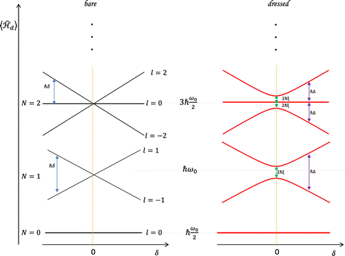
Figure 2. Left: The expectation values of the coupled Hamiltonian in the Fock states $|n_x,n_z⟩$, as given in (89(89) $$\begin{array}{c}\hfill ⟨{\widehat{\mathcal{H}}}_d⟩=\frac{ħ{\mathit{\omega }}_0}{2}(N+1)+\frac{ħ}{2}\mathit{\delta }l.\end{array}$$(89) ). These are the so-called ‘bare’ states of the system. Right: Expectation values of the coupled Hamiltonian in the ‘dressed’ states $|n_{\mathit{\alpha }}{n}_{\mathit{\beta }}⟩$. The effects of the dressing are the formation of an avoided crossing between the $l=n_z-n_x$ sub-levels of the system at the point $\mathit{\delta }=0$. The size of the splitting is dependent on the electric coupling field strength in (67(67) $$\begin{array}{c}\hfill E_p(t)=\text{Re}\left({\mathit{ϵ}}_p{e}^{i{\mathit{\omega }}_{p}t}\right)(x{\widehat{e}}_z+z{\widehat{e}}_x)\end{array}$$(67) ), where the renormalized strength $\mathit{\xi }$ is defined in Equation (76(76) $$\begin{array}{c}\hfill \mathit{\xi }=\frac{e}{4m}\frac{1}{\sqrt{{\mathit{\omega }}_1{\mathit{\omega }}_z}}{\mathit{ϵ}}_p.\end{array}$$(76) ) (not shown to scale).

5.2. Removing the time dependence and dressing

The explicit time dependence is removed from Hamiltonian (75(75) $$\begin{array}{cc}\hfill {\widehat{\mathcal{H}}}_p{}^{\prime }& =\widehat{\mathcal{H}}{}^{\prime }-e{\widehat{V}}_p^{\prime }(t)\hfill \\ \hfill & =ħ{\mathit{\omega }}_{+}\left({\widehat{a}}_x^{†}{\widehat{a}}_x+\frac{1}{2}\right)-ħ{\mathit{\omega }}_{-}\left({\widehat{a}}_y^{†}{\widehat{a}}_y+\frac{1}{2}\right)\hfill \\ \hfill & +ħ{\mathit{\omega }}_z\left({\widehat{a}}_z^{†}{\widehat{a}}_z+\frac{1}{2}\right)+ħ\mathit{\xi }\{{\widehat{a}}_z^{†}{\widehat{a}}_x{e}^{i{\mathit{\omega }}_{p}t}+{\widehat{a}}_x^{†}{\widehat{a}}_z{e}^{-i{\mathit{\omega }}_{p}t}\},\hfill \end{array}$$(75) ) by transformation to the Interaction picture [34], achieved by application of the unitary operator(77) $$\begin{array}{c}\hfill {\widehat{U}}_{\mathit{\delta }}^{\prime }(t)=exp\left\{-i\frac{{\mathit{\omega }}_p}{2}({\widehat{n}}_z-{\widehat{n}}_x)t\right\}.\end{array}$$(77)

This leads to(78) $$\begin{array}{cc}\hfill {\widehat{\mathcal{H}}}_{\mathit{pt}}{}^{\prime }& ={\widehat{U}}_{\mathit{\delta }}^{\prime }(t){\widehat{\mathcal{H}}}_p{}^{\prime }{\widehat{U}}_{\mathit{\delta }}^{\prime †}(t)+iħ{\widehat{\dot{U}}}_{\mathit{\delta }}^{\prime }(t){\widehat{U}}_{\mathit{\delta }}^{\prime †}(t)\hfill \\ \hfill & =ħ{\mathit{\omega }}_{+}\left({\widehat{a}}_x^{†}{\widehat{a}}_x+\frac{1}{2}\right)+ħ{\mathit{\omega }}_z\left({\widehat{a}}_z^{†}{\widehat{a}}_z+\frac{1}{2}\right)\hfill \\ \hfill & -ħ{\mathit{\omega }}_{-}\left({\widehat{a}}_y^{†}{\widehat{a}}_y+\frac{1}{2}\right)\hfill \\ \hfill & +ħ\mathit{\xi }({\widehat{a}}_x^{†}{\widehat{a}}_z+{\widehat{a}}_z^{†}{\widehat{a}}_x)+ħ\frac{{\mathit{\omega }}_p}{2}({\widehat{n}}_z-{\widehat{n}}_x).\hfill \end{array}$$(78)

The Hamiltonian ${\widehat{\mathcal{H}}}_{\mathit{pt}}{}^{\prime }$ is now rewritten in terms of operators of the dressed modes(79) $$\begin{array}{cc}& {\widehat{a}}_{\mathit{\alpha }}^{†}=cos\frac{\mathit{\theta }}{2}{\widehat{a}}_z^{†}-sin\frac{\mathit{\theta }}{2}{\widehat{a}}_x^{†},{\widehat{a}}_{\mathit{\alpha }}=cos\frac{\mathit{\theta }}{2}{\widehat{a}}_z-sin\frac{\mathit{\theta }}{2}{\widehat{a}}_x,\hfill \\ \hfill & {\widehat{a}}_{\mathit{\beta }}^{†}=cos\frac{\mathit{\theta }}{2}{\widehat{a}}_x^{†}+sin\frac{\mathit{\theta }}{2}{\widehat{a}}_z^{†},{\widehat{a}}_{\mathit{\beta }}=cos\frac{\mathit{\theta }}{2}{\widehat{a}}_x+sin\frac{\mathit{\theta }}{2}{\widehat{a}}_z,\hfill \end{array}$$(79)

where(80) $$\begin{array}{c}\hfill \mathit{\theta }=arctan\left[\frac{2\mathit{\xi }}{\mathit{\delta }}\right].\end{array}$$(80)

This produces(81) $$\begin{array}{cc}\hfill {\widehat{\mathcal{H}}}_{\mathit{pt}}^{\prime }& =ħ{\mathit{\epsilon }}_{\mathit{\alpha }}\left({\widehat{n}}_{\mathit{\alpha }}+\frac{1}{2}\right)+ħ{\mathit{\epsilon }}_{\mathit{\beta }}\left({\widehat{n}}_{\mathit{\beta }}+\frac{1}{2}\right)\hfill \\ \hfill & -ħ{\mathit{\omega }}_{-}\left({\widehat{a}}_y^{†}{\widehat{a}}_y+\frac{1}{2}\right),\hfill \end{array}$$(81)

with the frequencies of the dressed modes given by(82) $$\begin{array}{c}\hfill {\mathit{\epsilon }}_{\mathit{\alpha }}=\frac{({\mathit{\omega }}_{+}+{\mathit{\omega }}_z)+\mathrm{\Delta }}{2},{\mathit{\epsilon }}_{\mathit{\beta }}=\frac{({\mathit{\omega }}_{+}+{\mathit{\omega }}_z)-\mathrm{\Delta }}{2},\end{array}$$(82) (83) $$\begin{array}{c}\hfill \mathrm{\Delta }=\sqrt{4{\mathit{\xi }}^2+{\mathit{\delta }}^2}.\end{array}$$(83)

The ‘dressing’ by the oscillatory field (67(67) $$\begin{array}{c}\hfill E_p(t)=\text{Re}\left({\mathit{ϵ}}_p{e}^{i{\mathit{\omega }}_{p}t}\right)(x{\widehat{e}}_z+z{\widehat{e}}_x)\end{array}$$(67) ) is equivalent to a rotation through an angle $\mathit{\theta }$ around the local y-axis of the trap. This axis takes the form of the second component of a set of Schwinger boson operators formed from the operators of the x and z modes. This idea is further discussed in the following section.

5.3. The avoided crossing

In complete analogy to the angular momentum-like operators defined in (62(62) $$\begin{array}{cc}\hfill {\widehat{I}}_0& =\frac{ħ}{2}\left({\widehat{a}}_x^{†}{\widehat{a}}_x+{\widehat{a}}_y^{†}{\widehat{a}}_y\right),\hfill \\ \hfill {\widehat{I}}_1& =\frac{ħ}{2}\left({\widehat{a}}_x^{†}{\widehat{a}}_y+{\widehat{a}}_y^{†}{\widehat{a}}_x\right),\hfill \\ \hfill {\widehat{I}}_2& =-\frac{iħ}{2}\left({\widehat{a}}_x^{†}{\widehat{a}}_y-{\widehat{a}}_y^{†}{\widehat{a}}_x\right),\hfill \\ \hfill {\widehat{I}}_3& =\frac{ħ}{2}\left({\widehat{a}}_x^{†}{\widehat{a}}_x-{\widehat{a}}_y^{†}{\widehat{a}}_y\right),\hfill \end{array}$$(62) ), the following set $\underline{J}$ are defined:(84) $$\begin{array}{cc}\hfill {\widehat{J}}_0& =\frac{ħ}{2}\left({\widehat{a}}_z^{†}{\widehat{a}}_z+{\widehat{a}}_x^{†}{\widehat{a}}_x\right),\hfill \\ \hfill {\widehat{J}}_1& =\frac{ħ}{2}\left({\widehat{a}}_z^{†}{\widehat{a}}_x+{\widehat{a}}_x^{†}{\widehat{a}}_z\right),\hfill \\ \hfill {\widehat{J}}_2& =-\frac{iħ}{2}\left({\widehat{a}}_z^{†}{\widehat{a}}_x-{\widehat{a}}_x^{†}{\widehat{a}}_z\right),\hfill \\ \hfill {\widehat{J}}_3& =\frac{ħ}{2}\left({\widehat{a}}_z^{†}{\widehat{a}}_z-{\widehat{a}}_x^{†}{\widehat{a}}_x\right),\hfill \end{array}$$(84)

which obey the appropriate modification of the commutation relations (63(63) $$\begin{array}{c}\hfill \left[{\widehat{I}}_i,{\widehat{I}}_j\right]=iħ{\mathit{\epsilon }}_{\mathit{ijk}}{\widehat{I}}_k,\left[{\widehat{I}}_0,{\widehat{I}}_i\right]=0;\{i,j,k\}=1,2,3.\end{array}$$(63) ). The sign of the second and third components has been chosen such that(85) $$\begin{array}{c}\hfill {\widehat{J}}_2=\frac{1}{2}{\widehat{L}}_y\equiv \frac{1}{2}\left(\widehat{z}{\widehat{p}}_x-\widehat{x}{\widehat{p}}_z\right),\end{array}$$(85)

and in this way the set $\underline{J}$ is defined in the same sense of rotation as $\underline{I}$. The coupled Hamiltonian (78(78) $$\begin{array}{cc}\hfill {\widehat{\mathcal{H}}}_{\mathit{pt}}{}^{\prime }& ={\widehat{U}}_{\mathit{\delta }}^{\prime }(t){\widehat{\mathcal{H}}}_p{}^{\prime }{\widehat{U}}_{\mathit{\delta }}^{\prime †}(t)+iħ{\widehat{\dot{U}}}_{\mathit{\delta }}^{\prime }(t){\widehat{U}}_{\mathit{\delta }}^{\prime †}(t)\hfill \\ \hfill & =ħ{\mathit{\omega }}_{+}\left({\widehat{a}}_x^{†}{\widehat{a}}_x+\frac{1}{2}\right)+ħ{\mathit{\omega }}_z\left({\widehat{a}}_z^{†}{\widehat{a}}_z+\frac{1}{2}\right)\hfill \\ \hfill & -ħ{\mathit{\omega }}_{-}\left({\widehat{a}}_y^{†}{\widehat{a}}_y+\frac{1}{2}\right)\hfill \\ \hfill & +ħ\mathit{\xi }({\widehat{a}}_x^{†}{\widehat{a}}_z+{\widehat{a}}_z^{†}{\widehat{a}}_x)+ħ\frac{{\mathit{\omega }}_p}{2}({\widehat{n}}_z-{\widehat{n}}_x).\hfill \end{array}$$(78) ) before dressing is rewritten:(86) $$\begin{array}{cc}\hfill {\widehat{\mathcal{H}}}_{\mathit{pt}}^{\prime }& ={\mathit{\omega }}_0{\widehat{J}}_0+\mathit{\delta }{\widehat{J}}_3+2\mathit{\xi }{\widehat{J}}_1+\frac{ħ{\mathit{\omega }}_0}{2}\hfill \\ \hfill & -ħ{\mathit{\omega }}_{-}\left({\widehat{a}}_y^{†}{\widehat{a}}_y+\frac{1}{2}\right),\hfill \end{array}$$(86)

where ${\mathit{\omega }}_0={\mathit{\omega }}_{+}+{\mathit{\omega }}_z$. In order to examine only the coupled spectrum, the magnetron motion is dropped to form:(87) $$\begin{array}{cc}\hfill {\widehat{\mathcal{H}}}_d& ={\widehat{\mathcal{H}}}_{\mathit{pt}}^{\prime }+ħ{\mathit{\omega }}_{-}\left({\widehat{a}}_y^{†}{\widehat{a}}_y+\frac{1}{2}\right)\hfill \\ \hfill & ={\mathit{\omega }}_0{\widehat{J}}_0+\mathit{\delta }{\widehat{J}}_3+2\mathit{\xi }{\widehat{J}}_1+\frac{ħ{\mathit{\omega }}_0}{2}.\hfill \end{array}$$(87)

The quantum numbers $N=n_z+n_x$ and $l=n_z-n_x$ are defined so that [26]:(88) $$\begin{array}{cc}\hfill {\widehat{J}}_0|n_x,n_z⟩& =\frac{ħ}{2}N|n_x,n_z⟩,\hfill \\ \hfill {\widehat{J}}_3|n_x,n_z⟩& =\frac{ħ}{2}l|n_x,n_z⟩,\hfill \end{array}$$(88)

where $N=0,1,2,3,...,$ and $l=-N,-N+2,...,N-2,N.$ The expectation value of ${\widehat{\mathcal{H}}}_d$ in the Fock state $|n_x,n_z⟩$ is given by:(89) $$\begin{array}{c}\hfill ⟨{\widehat{\mathcal{H}}}_d⟩=\frac{ħ{\mathit{\omega }}_0}{2}(N+1)+\frac{ħ}{2}\mathit{\delta }l.\end{array}$$(89)

We similarly rewrite the dressed Hamiltonian (81(81) $$\begin{array}{cc}\hfill {\widehat{\mathcal{H}}}_{\mathit{pt}}^{\prime }& =ħ{\mathit{\epsilon }}_{\mathit{\alpha }}\left({\widehat{n}}_{\mathit{\alpha }}+\frac{1}{2}\right)+ħ{\mathit{\epsilon }}_{\mathit{\beta }}\left({\widehat{n}}_{\mathit{\beta }}+\frac{1}{2}\right)\hfill \\ \hfill & -ħ{\mathit{\omega }}_{-}\left({\widehat{a}}_y^{†}{\widehat{a}}_y+\frac{1}{2}\right),\hfill \end{array}$$(81) ):(90) $$\begin{array}{cc}\hfill {\widehat{\mathcal{H}}}_{\mathit{pt}}^{\prime }& =\frac{({\mathit{\epsilon }}_{\mathit{\beta }}+{\mathit{\epsilon }}_{\mathit{\alpha }})}{2}\left({\widehat{n}}_{\mathit{\beta }}+{\widehat{n}}_{\mathit{\alpha }}\right)+\frac{({\mathit{\epsilon }}_{\mathit{\beta }}-{\mathit{\epsilon }}_{\mathit{\alpha }})}{2}\left({\widehat{n}}_{\mathit{\beta }}-{\widehat{n}}_{\mathit{\alpha }}\right)\hfill \\ \hfill & +\frac{ħ{\mathit{\omega }}_0}{2}-ħ{\mathit{\omega }}_{-}({\widehat{a}}_y^{†}{\widehat{a}}_y+\frac{1}{2})\hfill \\ \hfill & ={\mathit{\omega }}_0{\widehat{J}}_0^{\mathit{\alpha }\mathit{\beta }}+\mathrm{\Delta }{\widehat{J}}_3^{\mathit{\alpha }\mathit{\beta }}+\frac{ħ{\mathit{\omega }}_0}{2}-ħ{\mathit{\omega }}_{-}\left({\widehat{a}}_y^{†}{\widehat{a}}_y+\frac{1}{2}\right),\hfill \end{array}$$(90)

where ${\widehat{J}}_0^{\mathit{\alpha }\mathit{\beta }}$ and ${\widehat{J}}_3^{\mathit{\alpha }\mathit{\beta }}$ are the zeroth and third components of the set of Schwinger boson operators of the dressed modes of the coupled x and z motions. Dropping the magnetron contribution to define ${\widehat{\mathcal{H}}}_d$ in terms of the set ${\underline{J}}^{\mathit{\alpha }\mathit{\beta }}$:(91) $$\begin{array}{c}\hfill {\widehat{\mathcal{H}}}_d={\mathit{\omega }}_0{\widehat{J}}_0^{\mathit{\alpha }\mathit{\beta }}+\mathrm{\Delta }{\widehat{J}}_3^{\mathit{\alpha }\mathit{\beta }}+\frac{ħ{\mathit{\omega }}_0}{2}.\end{array}$$(91)

Comparing (87(87) $$\begin{array}{cc}\hfill {\widehat{\mathcal{H}}}_d& ={\widehat{\mathcal{H}}}_{\mathit{pt}}^{\prime }+ħ{\mathit{\omega }}_{-}\left({\widehat{a}}_y^{†}{\widehat{a}}_y+\frac{1}{2}\right)\hfill \\ \hfill & ={\mathit{\omega }}_0{\widehat{J}}_0+\mathit{\delta }{\widehat{J}}_3+2\mathit{\xi }{\widehat{J}}_1+\frac{ħ{\mathit{\omega }}_0}{2}.\hfill \end{array}$$(87) ) and (91(91) $$\begin{array}{c}\hfill {\widehat{\mathcal{H}}}_d={\mathit{\omega }}_0{\widehat{J}}_0^{\mathit{\alpha }\mathit{\beta }}+\mathrm{\Delta }{\widehat{J}}_3^{\mathit{\alpha }\mathit{\beta }}+\frac{ħ{\mathit{\omega }}_0}{2}.\end{array}$$(91) ), it is straightforward to see the effects of this ‘dressing’: the degeneracy of the l levels at the point $\mathit{\delta }=0$ is lifted by the non-zero value of $\mathrm{\Delta }=\sqrt{4{\mathit{\xi }}^2+{\mathit{\delta }}^2}$. This is shown pictorially in Figure 2, where the expectation values of the bare and dressed Hamiltonians have been plotted as a function of $\mathit{\delta }$ for the first few total quantum numbers N. The plot shows how an avoided crossing occurs at the point $\mathit{\delta }=0$ due to the dressing of the modes [28]. The size of the splitting is given by $2ħ\mathit{\xi }$, and accordingly varies with the strength of the applied field in (67(67) $$\begin{array}{c}\hfill E_p(t)=\text{Re}\left({\mathit{ϵ}}_p{e}^{i{\mathit{\omega }}_{p}t}\right)(x{\widehat{e}}_z+z{\widehat{e}}_x)\end{array}$$(67) ). In comparing the results of the above quantum calculation to the classical one in [29], it is clear that the dressed-atom formalism is directly applicable to the quantum system.

It is convenient to describe the coupling as taking place between the axial and cyclotron energy levels, which is logical language based on the ladder diagrams that can be drawn for the independent harmonic oscillator modes of the Penning trap [1]. The above analysis however, reveals that it is more appropriate to describe the coupling as taking place between the combined sub-levels, l, of the system. This can be seen explicitly in the figure, as the avoided crossings take place between adjacent values of l. In the present case, there are N avoided crossings formed at the point $\mathit{\delta }=0$ for each N when the system is dressed.

5.4. The dressed-atom formalism in the Penning trap

The realization of the dressed levels and the formation of the avoided crossing in the above calculation results from treating the cyclotron and axial modes as a combined system. The simple structure of the Penning trap Hamiltonian (19(19) $$\begin{array}{cc}\hfill \widehat{\mathcal{H}}& =ħ{\mathit{\omega }}_{+}\left({\widehat{a}}_{+}^{†}{\widehat{a}}_{+}+\frac{1}{2}\right)-ħ{\mathit{\omega }}_{-}\left({\widehat{a}}_{-}^{†}{\widehat{a}}_{-}+\frac{1}{2}\right)\hfill \\ \hfill & +ħ{\mathit{\omega }}_z\left({\widehat{a}}_z^{†}{\widehat{a}}_z+\frac{1}{2}\right).\hfill \end{array}$$(19) ) can be exploited, and the system treated as three, two-dimensional sub-systems, each with its own Schwinger boson algebra, in a consistent way. This allows exploration of dressed-atom techniques [25] within the Penning trap in general, and offers new possibilities in terms of theoretical investigation. For example, a simple modification of the coupling frequency in (67(67) $$\begin{array}{c}\hfill E_p(t)=\text{Re}\left({\mathit{ϵ}}_p{e}^{i{\mathit{\omega }}_{p}t}\right)(x{\widehat{e}}_z+z{\widehat{e}}_x)\end{array}$$(67) ) can produce a Penning trap Hamiltonian of a Landau-Zener-Stückelberg system [39,40]. Fourier transforms of the interference patterns resulting from the induced driving of this Hamiltonian can extract information on the energy level spectrum, and can provide a tool with which to study the interaction of the system with the trapping fields and with the environment [41]. Such capabilities in the Penning trap have obvious appeal.

Furthermore, the treatment of the calculation in the $\{x,y\}$ basis following from Section 4 enables direct access to the spatial degrees of freedom in the trap through this well-known experimental technique. Through this, manipulation of the trapping potential, without modification of the basic trap design, is an ongoing topic of investigation.

6. Summary

In this paper, we closely examined the processes used to solve the Penning trap Hamiltonian. In order to keep track of the individual dynamics of the x and y motions in a consistent way, it was shown how the transformation of the canonical coordinates should take place after quantization. The frame rotating around the z-axis, conventionally used to achieve this, was shown to lead to inconsistent results in the quantum regime in Section 3. This promoted the use of a set of Schwinger boson angular momentum operators in the Penning trap, and inspired the results of the quantum avoided crossing in the mode coupling calculation in Section 5. The treatment demonstrates how such techniques can be employed in further calculation, offering new possibilities of theoretical and experimental research in the Penning trap.

Acknowledgements

We dedicate this contribution to the memory of Professor Danny Segal: a colleague and expert in Penning trap research.

Additional information

Funding

This work was supported by the UK Engineering and Physical Sciences Research Council [grant number EP/K503198/1].

Notes

No potential conflict of interest was reported by the authors.

References

- Brown, L.S.; Gabrielse, G. Geonium Theory: Physics of a Single Electron or Ion in a Penning Trap. Rev. Modern Phys. 1986, 58, 233–311.
- Kretzschmar, M. Particle Motion in a Penning Trap. Eur. J. Phys. 1991, 12, 240–246.
- Kretzschmar, M. Single Particle Motion in a Penning Trap: Description in the Classical Canonical Formalism. Phys. Scr. 1992, 46, 544–554.
- Kretzschmar, M. Theory of the Elliptical Penning Trap. Int. J. Mass Spectrom. 2008, 275, 21–33.
- Hanneke, D.; Fogwell, S.; Gabrielse, G. New Measurement of the Electron Magnetic Moment and the Fine Structure Constant. Phys. Rev. Lett. 2008, 100, 120801. arXiv: 0801.1134.
- Sturm, S.; Köhler, F.; Zatorski, J.; Wagner, A.; Harman, Z.; Werth, G.; Quint, W.; Keitel, C.H.; Blaum, K. High-precision Measurement of the Atomic Mass of the Electron. Nature 2014, 506, 467–470.
- Ciaramicoli, G.; Marzoli, I.; Tombesi, P. Trapped Electrons in Vacuum for a Scalable Quantum Processor. Phys. Rev. A 2004, 70, 032301.
- Lamata, L.; Porras, D.; Cirac, J.I.; Goldman, J.; Gabrielse, G. Towards Electron-electron Entanglement in Penning Traps. Phys. Rev. A 2010, 81, 022301. arXiv: 0905.0644.
- Mavadia, S.; Goodwin, J.F.; Stutter, G.; Bharadia, S.; Crick, D.R.; Segal, D.M.; Thompson, R.C. Control of the Conformations of Ion Coulomb Crystals in a Penning Trap. Nat. Commun. 2013, 4, 2571–2577.
- Cridland, A.; Lacy, J.; Pinder, J.; Verdú, J. Single Microwave Photon Detection with a Trapped Electron. Photonics 2016, 3, 59–73.
- Marzoli, I.; Tombesi, P.; Ciaramicoli, G.; Werth, G.; Bushev, P.; Stahl, S.; Schmidt-Kaler, F.; Hellwig, M.; Henkel, C.; Marx, G.; Jex, I.; Stachowska, E.; Szawiola, G.; Walaszyk, A. Experimental and Theoretical Challenges for the Trapped Electron Quantum Computer. J. Phys. B 2009, 42, 154010–154020.
- Ciaramicoli, G.; Marzoli, I.; Tombesi, P. Scalable Quantum Processor with Trapped Electrons. Phys. Rev. Lett. 2003, 91, 017901.
- Pedersen, L.H.; Rangan, C. Controllability and Universal Three-qubit Quantum Computation with Trapped Electron States. Quant. Inform. Process. 2008, 7, 33–42.
- Ciaramicoli, G.; Marzoli, I.; Tombesi, P. Realization of a Quantum Algorithm Using a Trapped Electron. Phys. Rev. A 2001, 63, 052307.
- Mancini, S.; Martins, A.M.; Tombesi, P. Quantum Logic with a Single Trapped Electron. 2008. arXiv: 9912008v1.
- Van Dyck, R.S.; Schwinberg, P.B.; Dehmelt, H.G. New High-precision Comparison of Electron and Positron g Factors. Phys. Rev. Lett. 1987, 59, 26–29.
- Lloyd, S. Quantum Illumination. Science 2008, 321, 1463. arXiv: 0803.2022.
- Tan, S.H.; Erkmen, B.I.; Giovannetti, V.; Guha, S.; Lloyd, S.; Maccone, L.; Pirandola, S.; Shapiro, J.H. Quantum Illumination with Gaussian States. Phys. Rev. Lett. 2008, 101, 253601–253604.
- Weedbrook, C.; Pirandola, S.; Cerf, N.J.; Ralph, T.C. Gaussian Quantum Information, 2011, arXiv:1110.3234v1.
- Shapiro, J.H.; Lloyd, S. Quantum Illumination versus Coherent-state Target Detection. New J. Phys. 2009, 11, 063045–063049.
- Guha, S.; Erkmen, B.I. Gaussian-state Quantum-illumination Receivers for Target Detection. Phys. Rev. A 2009, 80, 052310, arXiv: 0911.0950.
- Barzanjeh, S.; Guha, S.; Weedbrook, C.; Vitali, D.; Shapiro, J.H.; Pirandola, S. Microwave Quantum Illumination. Phys. Rev. Lett. 2015, 114, 080503.
- Verdú, J. Theory of the Coplanar-waveguide Penning Trap. New J. Phys. 2011, 13, 113029–113046.
- Pinder, J.; Verdú, J. A Planar Penning Trap with Tunable Dimensionality of the Trapping Potential. Int. J. Mass Spectrom. 2013, 356, 49–59.
- Garraway, B.M.; Perrin, H. Recent Developments in Trapping and Manipulation of Atoms with Adiabatic Potentials. J. Phys. B 2016, 49, 172001–1720021.
- Schwinger, J. On Angular Momentum; Dover Publications: New York, 1965.
- Kretzschmar, M. Octupolar Excitation of Ion Motion in a Penning Trap: A Theoretical Study. Int. J. Mass Spectrom. 2014, 357, 1–21.
- Dalibard, J.; Cohen-Tannoudji, C. Dressed-atom Approach to Atomic Motion in Laser Light: The Dipole Force Revisited. J. Opt. Soc. Amer. B 1985, 2, 1707–1720.
- Cornell, E.A.; Weisskoff, R.M.; Boyce, K.R.; Pritchard, D.E. Mode Coupling in a Penning Trap: π Pulses and a Classical Avoided Crossing. 1990, 41, 312–315.
- Jackson, J.D. Classical Electrodynamics, Wiley: New York, 1962.
- Wineland, D.; Dehmelt, H. Line Shifts and Widths of Axial, Cyclotron and G-2 Resonances in Tailored, Stored Electron (Ion) Cloud. Int. J. Mass Spectrom. Ion Phys. 1975, 16, 338–342.
- Bhaduri, R.K.; Li, S.; Tanaka, K.; Waddington, J.C. Quantum Gaps and Classical Orbits in a Rotating Two-dimensional Harmonic Oscillator. J. Phys. A: Gen. Phys. 1994, 27, 553–558.
- Landau, L.D.; Lifshitz, E.M. Quantum Mechanics: Non-relativistic Theory. Vol. 3; Course of Theoretical Physics; Butterworth-Heinemann: Oxford, 1977.
- Barnett, S.; Radmore, P. Methods in Theoretical Quantum Optics; Oxford University Press: New York, 2002.
- Schrödinger, E. E. Der stetige Übergang von der Mikro- zur Makromechanik. Die Naturwiss. 1926, 14, 664–666.
- Weihs, G.; Zeilinger, A. Photon Statistics at Beam Splitters: An Essential Tool in Quantum Information and Teleportation; Wiley, 2001, arXiv:1201.6120v1.
- Knoop, M.; Madsen, N.; Thompson, R.C. Physics with Trapped Charged Particles, Imperial College Press: London, 2014.
- Cohen-Tannoudji, C.; Reynaud, S. Dressed-atom Description of Resonance Fluorescence and Absorption Spectra of a Multi-level Atom in an Intense Laser Beam. J. Phys. B. 1977, 10, 345–363.
- Landau, L. The Theory of Energy Exchange in Collisions. Phys. Z. Sowjetunion. 1932, 1, 88–98.
- Stückelberg, E. Theory of Inelastic Collisions between Atoms. Helv. Phys. Acta 1932, 5, 369–423.
- Shevchenko, S.N.; Ashhab, S.; Nori, F. Landau-Zener-St{\"u}ckelberg Interferometry. Phys. Rep. 2010, 492, 1–30, arXiv:0911.1917v3.