Linearity performance analysis of the differential wavefront sensing for the Taiji programme

ABSTRACT

The Taiji programme is a Chinese space-based laser interferometer gravitational wave detection mission and the differential wavefront sensing (DWS) technique is introduced to reduce the effect of the laser pointing noise. As the distance between two adjacent satellites is about $3\times {10}^6\text{km}$, the wavefront of the receiving beam is a flat top beam. In this paper, we construct an analytical model of the DWS signal under the circumstances of Gaussian beam-flat top beam interference and study the linearity performance. The position offset of the beams is found to greatly affect the linearity range. A numerical method is used to simulate the linearity range of the DWS signal under various operating conditions. The linearity range decrease with the increase of the offset angle of the Gaussian beam and the offset length of the flat top beam. The offset range of the beams based on the requirement of the Taiji is given at last.

KEYWORDS:

• Gravitational wave
• laser interferometer
• differential wavefront sensing
• flat top beam

1. Introduction

In 2016, the American ground-based laser interferometer gravitational wave observatory (LIGO) announced the first direct detection of gravitational waves. The exciting news promoted China to propose its space-based gravitational wave detection programme, the Taiji programme, for reaching a wider range of gravitational radiation sources [1–4]. Compared with the ground-based programmes, the Taiji programme has to construct the inter-satellite laser link constellation with the help of a laser acquisition system. The system uses star trackers and CCD detectors to suppress the laser pointing error from $100\text{μ}\text{rad}$ to $1\text{μ}\text{rad}$ [5–8]. However, the satellite jitter caused by the solar wind, solar radiation, cosmic rays and other space environment hinders the acquirement of the scientific data. The drag free system suppresses such noise extensively, but the residual jitter is still coupled to the propagating laser and dominates the ranging noise. In order to reduce the detection error caused by the pointing jitter while taking into account redundancy, the Taiji programme plans to adopt the precision pointing system to achieve the pointing stability of $1\text{nrad}/\sqrt{\text{Hz}}$ in the frequency band within $1\text{mHz}-1\text{Hz}$. The precision pointing system is based on the Differential Wavefront Sensing (DWS) technique [9].

The core concept of the DWS technique is to obtain the included angle of two beams by reading the phase difference between different quadrants of a quadrant photodetector (QPD) [10–12]. With the advantages of high sensitivity and low noise, the DWS technique is now widely used for precision angle measurement while many theoretical explorations and experimental studies on this technique have been done. In 2010, Hechenblaikner [13] constructed an analytical model of the DWS for Gaussian beam-Gaussian beam interference. In 2012, Sheard [14] gave an approximate phase-angle conversion formula of plane beam-Gaussian beam interference for the GRACE Follow-on programme. In 2014, Yuhui Dong [15] conducted principle demonstration experiment of precision angle measurement system with two Gaussian beams and verified the feasibility of the DWS technique. In 2016, Huizong Duan [16] improved the analytical model of Hechenblaikner by involving beam clipping and beam walking into the model. In addition, he also built a numerical model under an ideal condition and got the conclusion that the larger the beam clipping is, the smaller the non-linearity is.

Most of the studies of the DWS technique concentrate on the interference between Gaussian beams for simplification. However, the preliminary design of the distance between the two adjacent Taiji satellites is $3\times {10}^6\text{km}$. After spreading such a long distance, the wavefront of the propagating light at the receiving aperture will have the properties of a flat top beam. Therefore, the study of the DWS technique under the condition of flat top beam-Gaussian beam interference is essential for the Taiji programme. However, the DWS between a Gaussian and a flat top beam is not as well studied with only a few investigations done within the LISA community. Ideally, the Gaussian beam perpendicularly enters the QPD centre for obtaining high interference efficiency in all the four quadrants. It can be fulfilled by correcting the position of the laser spot on the QPD surface with the help of a ground-based assembly rectify system. However, in practice, the assembly errors will make the beam offset from the centre. On the other hand, the flat top beam may deviate from the QPD centre because of satellites jitter. A dedicated imaging system is used to suppress the offset, but the residual offset still exists. The position offset of the beams greatly affects the linearity range of the DWS technique. Therefore, the permissible offset range is also significant to the design of the Taiji programme.

This paper is structured as follows: Based on the physical model of the wavefront distribution [17,18], an analytical model of the DWS signal under the condition of flat top beam-Gaussian beam interference is presented. The analytical expression is different from the result derived from two Gaussian beams [13,16] and is used to qualitatively analyse the influence of beam offset to the linearly performance. Then, a numerical method is involved for quantitative analysis the effect of beam offset under four basic practical situations. Based on the numerical results we present the offset range of the beams which can fulfil the requirement of the Taiji programme.

2. Analytical expression of the DWS signal

In order to obtain the analytical expression of the DWS signal, we need to establish the physical model of the wavefront of the Gaussian beam and the flat top beam. In the coordinate system where the laser emission point is the origin and the propagation direction is the z-axis, the complex amplitude of the local Gaussian beam can be expressed as, (1) $A_{\text{Gaussian}}=\sqrt{\frac{2P}{\pi \cdot {\omega }_g^2(z)}}\cdot e^{-\frac{x^2+y^2}{{\omega }_g^2(z)}}\cdot e^{-ik\frac{x^2+y^2}{2R(z)}-i\eta (z)-ikz}$(1) where, $P$ is the laser power, $z$ is the propagation distance of the beam, $\eta$ is the Gouy phase, ${\omega }_g(z)$ and $R(\text{z})$ represent the spot radius and the curvature radius, respectively.

The receiving beam from the remote satellite can be seen as a flat top beam at the receiving aperture. After being clipped by the telescope, the complex amplitude of the beam is given by, (2) $A_{\text{flat - top}}=\{\begin{array}{l}\begin{array}{cc}{E}_0\times e^{-ikz}& \text{for }\mathrm{\forall }x,y\text{fullfils}{x}^2+y^2\le {\omega }^2\end{array}\\ \begin{array}{cc}0& \text{elses}\end{array}\end{array}$(2) where, $E_0$ stands for the beam amplitude and $\omega$ is the spot radius on the QPD.

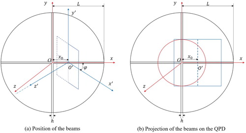
We suppose that the Gaussian beam perpendicularly enters the QPD centre and the flat top beam only has an offset in the yaw direction with the offset length of $x_0$, the offset angle of $\phi$ (it is also the included angle of the two beams). Because of the symmetric distribution of the wavefront in the top and bottom quadrants, the offset of the beam will only influence the DWS signal of left and right quadrants. For simplifying the calculation, it is assumed that the flat top beam is clipped by a square aperture. Compared with a circular aperture in the actual situation, we only ignore few additional integral areas in the edge, where the interference intensity is relatively weaker. The following analysis results will prove the validity of the assumption.

Figure 1(a) is the schematic diagram of the above situation. The Gaussian beam and the flat top beam propagate in the negative direction of z-axis and z′-axis, respectively. The transformation formula between the coordinate $(x,y,z)$ and the coordinate $(x^{\mathrm{\prime }},y^{\mathrm{\prime }},z^{\mathrm{\prime }})$ can be written as, (3) $\begin{array}{rl}\left(\begin{array}{c}{x}^{\mathrm{\prime }}\\ y^{\mathrm{\prime }}\\ z^{\mathrm{\prime }}\end{array}\right)& =\left(\begin{array}{ccc}\cos \phi & 0& \sin \phi \\ 0& 1& 0\\ -\sin \phi & 0& \cos \phi \end{array}\right)\left(\begin{array}{c}x\\ y\\ z\end{array}\right)\\ & +\left(\begin{array}{c}-x_0\cos \phi \\ 0\\ x_0\sin \phi \end{array}\right)\end{array}$(3) Therefore, the complex amplitude of the flat top beam can be expressed in the coordinate $(x,y,z)$ as $A_{\text{flat - top}}^{\mathrm{\prime }}$. Figure 1(b) shows the projection of the beams on the QPD surface.

Figure 1. Diagram of the coordinate system. (a) shows the position of the beams, in which $(x,y,z)$ and $(x^{\mathrm{\prime }},y^{\mathrm{\prime }},z^{\mathrm{\prime }})$ are the coordinate of the Gaussian beam and the flat top beam respectively. Where, $h$ stands for the gap of the QPD, $L$ represents the radius of the detector, $x_0$ is the offset length of the flat top beam and $\phi$ is the offset angle. (b) presents the projection of the beams on the QPD surface.

Let $z_g$ and $z_f$ represent the propagation distance of the Gaussian beam and the flat top beam from the emission point to the detector respectively. We make ${\omega }_f$ stand for the half length of the flat top optical spot on the detector (${\omega }_f$ is set equal to ${\omega }_g$ for obtaining high interference contrast). Therefore, the complex amplitude of the interference pattern on the left half of the QPD is given by, (4) $\begin{array}{rl}{F}_{\text{left}}& ={\int }_{S_{\text{left}}}dS\cdot A_{\text{Gaussian}}{A}_{\text{flat - top}}^{\mathrm{\prime }\ast }\\ & ={\int }_{-{\omega }_f}^{{\omega }_f}dy{\int }_{x_0-\frac{{\omega }_f}{\cos \phi }}^{-h}dx\cdot A_{\text{Gaussian}}{A}_{\text{flat - top}}^{\mathrm{\prime }\ast }\end{array}$(4) where, $S_{\text{left}}$ stands for the integral area of the left quadrant. Then we introduce $C_1$ and $C_2$ as, (5) $\begin{array}{cc}{C}_1=\frac{1}{{\omega }_g^2(z_g)}+\frac{ik}{2R(z_g)}& C_2=ik\sin \phi \end{array}$(5) After substituting equation (1) and (2), the complex amplitude can be rewritten as, (6) $\begin{array}{rl}{F}_{\text{left}}& =\frac{P(y)\cdot \exp (\frac{{C_2}^2}{4C_1})}{\sqrt{C_1}}\\ & \times \{\text{erf}\left[\sqrt{C_1}\left(\frac{{\omega }_f}{\cos \phi }-x_0+\frac{C_2}{2C_1}\right)\right]\\ & -\text{erf}\left[\sqrt{C_1}\left(h+\frac{C_2}{2C_1}\right)\right]\}\end{array}$(6) where, (7) $\begin{array}{rl}P(y)& ={\int }_{-{\omega }_f}^{{\omega }_f}\sqrt{\frac{2P}{\pi {\omega }_g^2(z_g)}}\\ & E_0{e}^{-i\eta (z)}\cdot e^{ik(z_f-z_g-x_0\sin \phi )}\cdot e^{-\left[\frac{1}{{\omega }_g^2(z_g)}+\frac{ik}{2R(z_g)}\right]y^2}dy\end{array}$(7) Similarly, the complex amplitude of the interference pattern on the right half of the QPD is given by, (8) $\begin{array}{rl}{F}_{\text{right}}& =\frac{P(y)\cdot \exp \left(\frac{{C_2}^2}{4C_1}\right)}{\sqrt{C_1}}\\ & \times \{\text{erf}\left[\sqrt{C_1}\left(\frac{{\omega }_f}{\cos \phi }+x_0-\frac{C_2}{2C_1}\right)\right]\\ & -\text{erf}\left[\sqrt{C_1}\left(h-\frac{C_2}{2C_1}\right)\right]\}\end{array}$(8) Therefore, the analytical expression of the DWS signal is written as, (9) $\begin{array}{r}\text{DWS}=\arg \left\{\frac{\begin{array}{c}\text{erf}\left[\sqrt{C_1}\left(\frac{{\omega }_f}{\cos \phi }+x_0-\frac{C_2}{2C_1}\right)\right]\\ -\text{erf}\left[\sqrt{C_1}\left(h-\frac{C_2}{2C_1}\right)\right]\end{array}}{\begin{array}{c}\text{erf}\left[\sqrt{C_1}\left(\frac{{\omega }_f}{\cos \phi }-x_0+\frac{C_2}{2C_1}\right)\right]\\ -\text{erf}\left[\sqrt{C_1}\left(h+\frac{C_2}{2C_1}\right)\right]\end{array}}\right\}\end{array}$(9) From equation (9), we know that the DWS signal is the function of the included angle, the gap of the QPD, the size of optical spots and the offset length of the flat top beam. The analytical expression is quite different from the result derived from two Gaussian beams [13]. The results in [16] show that the radius of the QPD has a strong influence on the DWS signal of two Gaussian beams. However, the size of the flat top beam rather than the QPD size has effect to the DWS signal with the flat top beam and the Gaussian beam interference. Thus, the derived result (9) is more effective for analysing the performance of the DWS in the Taiji programme.

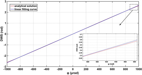
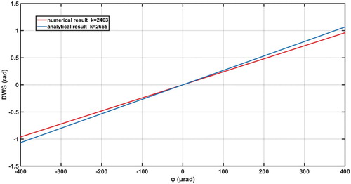
In the Taiji programme, the preliminary design of the QPD and the spot size are ${\omega }_f=0.5\text{mm},h=25\text{μ}\text{m},L=1\text{mm}$. These parameters will be used in the subsequent parts of this paper. Calculated from equation (9), the blue curve in Figure 2 presents the relationship between $\phi$ and the DWS signal when we suppose $x_0=0\text{μ}\text{m}$. For studying the linearity performance of the DWS signal, the linear fitting curve is also drawn in the same figure. We can get the conclusion that the linearity of the DWS signal deteriorates with the increase of the included angle.

Figure 2. The comparison of the analytical result and the linear fitting result. Red curve: the relationship between $\phi$ and the DWS signal with $x_0=0\text{μ}\text{m}$. Blue curve: the linear fitting curve.

The non-linearity of the DWS signal will lead to angle measurement error. Although the error will be gradually eliminated by the control loop, it will still affect the scientific data during the control process. As already mentioned in the first chapter, the requirement of the precision pointing system of the Taiji programme is to achieve pointing accuracy of $1\text{nrad}/\sqrt{\text{Hz}}$ within the pointing deviation range of $\pm 1\text{μ}\text{rad}$. With the sampling frequency of $3.3\text{Hz}$, the root mean square value of the pointing error should be lower than approximately $3\text{nrad}$. When we consider a certain degree of redundancy for the whole programme, the measurement error caused by the DWS technique need to be lower than $1\text{nrad}$ in the time domain. Based on the preliminary design, the telescope aperture is approximately $30\text{cm}$ and the optical spot diameter on the QPD surface is $1\text{mm}$, that is, the optical imaging system reduces the optical spot size of the flat top beam by $300$ times. Therefore, the offset angle increases $300$ times at the same time. As a result, within the deviation angle range of $\pm 300\text{μ}\text{rad}$, only if the absolute measurement error of the included angle ($\mathrm{\Delta }\phi$) induced by the non-linear part of the DWS technique is less than $300\text{nrad}$, can the requirement of the Taiji programme be fulfilled. 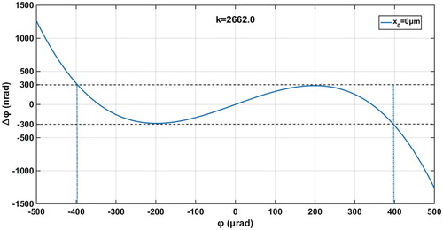That is, (10) $\begin{array}{rl}|\mathrm{\Delta }\phi (\phi )|& =\left|\frac{\text{DWS}(\phi )}{k}-\phi \right|\le 300\text{nrad}\\ & \text{for}\mathrm{\forall }\phi \in [-300\text{μ}\text{rad},300\text{μ}\text{rad}]\end{array}$(10) where, $k$ is the slope of the linear fitting curve. Figure 3 shows the relationship between the absolute measurement error of the included angle and the offset angle with $x_0=0\text{μ}\text{m}$. As the curve is central symmetric about the origin, the linearity range satisfying formula (9) can be introduced as $\pm {\phi }_l$. It can be seen that ${\phi }_l$ is approximately $400\text{μ}\text{rad}$. Thus, the linear range can fulfil the requirement when both beams project onto the QPD centre.

Figure 3. The relationship between $\mathrm{\Delta }\phi (\phi )$ and $\phi$ with $x_0=0\text{μ}\text{m}$.

For studying the influence of the position offset to the linearity of the DWS signal, we calculate the linearity range $\pm {\phi }_l$ as well as the fitting factor $k$ with different value of $x_0$. The results are shown in Figure 4.

Figure 4. Red curve: the relationship between $x_0$ and ${\phi }_l$. Blue curve: the relationship between $x_0$ and $k$.

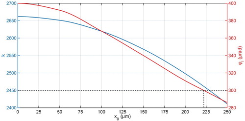
It can be concluded that increasing the offset length of the flat top beam will reduce the linearity range as well as the fitting factor. This is basically due to the fact that the difference between the left and right half-domains increases with the increase of the offset length. When the offset length increases to $225\text{μ}\text{m}$, the linearity range will be less than $\pm 300\text{μ}\text{rad}$. The analytical model reveals the essence of the DWS signal with Gaussian beam-flat top interference and shows the influence of the beam position offset to the linearity range. However, the square clipped assumption will bring calculation error when we confirm the offset range of the beams in the practical situation of the Taiji programme. On the other hand, we only obtain the analytical result with the flat top beam offsetting in only one direction. In other conditions, the analytical expression can hardly be obtained because it is difficult to decouple the two orthogonal directions. In the next section, the numerical method will be used to overcome these problems.

3. Linearity performance of the DWS technique under practical situations

We have already deduced the analytical expression in the last section. The conclusions are useful for qualitative analysis. In this section, the numerical method is firstly used to explore the linearity performance of the DWS technique under four basic practical situations with a circular clipped flat top beam. Then, the offset range of the beams is given through synthetically considering of all the cases. Following is the cases: (1) The Gaussian beam perpendicularly enters the centre of the detector while the flat top beam only has an offset in the yaw direction. (2) The Gaussian beam perpendicularly enters the centre of the detector while the flat top beam has an offset in both the yaw and the pitch direction. (3) Both the Gaussian beam and the flat top beam have an offset in the yaw direction. (4) The Gaussian beam has an offset in the pitch direction while the flat top beam has an offset in the yaw direction. More complex situations may also exist but can be seen as the combination of the above four cases.

3.1. Case 1: the Gaussian beam perpendicularly enters the QPD centre while the flat top beam only has an offset in the yaw direction

If the assembly errors of the QPD and the laser are small enough, the offset of the Gaussian beam from the centre of the detector can be ignored. Case 1 is similar with the situation in the last chapter with the only difference that the flat top beam is circular clipped here. It is still supposed that the offset length is $x_0$ and the offset angle is $\phi$ in the yaw direction.

The red curve in Figure 5 is the result of the numerical method with $x_0=0\text{μ}\text{m}$ while the blue curve is the analytical result with the same parameters. The linearity performance and the slope of the two curves are similar. Therefore, the square clipped approximation used in the analytical expression calculation will not lead to a wrong qualitative conclusion.

Figure 5. Blue curve: the relationship between $\phi$ and the DWS signal with circular clipped flat top beam. Red curve: the relationship between $\phi$ and the DWS signal with square clipped flat top beam.

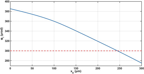
Based on the numerical method, Figure 6 shows the relationship between the linearity range $\pm {\phi }_l$ and the offset length $x_0$ in this case. The conclusion obtained here is same with the results given by the analytical model, that is, $\phi$ decreases with the increase of $x_0$. For satisfying the linearity range of $\pm 300\text{μ}\text{rad}$, the offset length should be guaranteed within $240\text{μ}\text{m}$.

Figure 6. The relationship between ${\phi }_l$ and $x_0$ in case 1.

3.2. Case 2: the Gaussian beam perpendicularly enters the QPD centre while the flat top beam has an offset in both the pitch and the yaw direction

In this case, the flat top beam has two offset directions. In the yaw direction, the offset length is $x_0$ and the offset angle is ${\phi }_x$. And in the pitch direction, the offset length is $y_0$ and the offset angle is ${\phi }_y$. Obviously, if we only change the offset in the yaw direction, the same conclusion with case 1 will be obtained. And if only the offset in the pitch direction is changed, the DWS signal of left and right quadrants will be unchanged. But the joint action of both directions may generate a different result. Firstly, we keep the value of $x_0$ and ${\phi }_y$ unchanged and give $y_0$ different values. Then, we just change the value of ${\phi }_y$ with invariant $x_0$ and $y_0$. The results of the linearity range are shown in Figure 7, respectively. As the linearity range is no longer origin-symmetric, ${\phi }_l$ represents the smaller boundary here.

Figure 7. Blue curve: the relationship between ${\phi }_l$ and $y_0$ with $x_0=10\text{μ}\text{m},{\phi }_y=10\text{μ}\text{rad}$. Red curve: the relationship between ${\phi }_l$ and ${\phi }_y$ with $x_0=10\text{μ}\text{m},y_0=10\text{μ}\text{m}$.

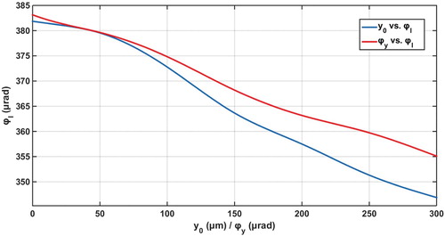
We can draw the conclusion that increasing the offset length or offset angle in the pitch direction will decrease the linearity range of the left and right quadrants DWS signal. This is due to the fact that when the centre of the flat top optical spot is not on the y-axis, the wavefront distribution of left and right quadrants is no longer the same.

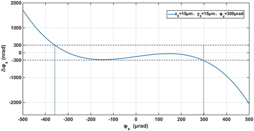
As required by the Taiji programme, the maximum potential offset angle in the pitch direction is also $300\text{μ}\text{rad}$. Therefore, to explore the maximum allowable offset length, we suppose ${\phi }_y=300\text{μ}\text{rad}$ and increase $x_0$ and $y_0$ at the same time. We make $\mathrm{\Delta }{\phi }_x$ stands for the measurement error of the induced angle in the yaw direction. Figure 8 presents the relationship between ${\phi }_x$ and $\mathrm{\Delta }{\phi }_x$ with $x_0=15\text{μ}\text{m},y_0=15\text{μ}\text{m}$. Here, the upper bound of the linearity range reaches $300\text{μ}\text{rad}$. Continue increasing $x_0$ and $y_0$ will make the linearity range less than the requirement. Therefore, the offset length of the flat top beam in the pitch and the yaw direction should not exceed $15\text{μ}\text{m}$.

Figure 8. The relationship between ${\phi }_x$ and $\mathrm{\Delta }{\phi }_x$. Where, $x_0=15\text{μ}\text{m},y_0=15\text{μ}\text{m},{\phi }_y=300\text{μ}\text{rad}$.

3.3. Case 3: both the Gaussian beam and the flat top beam have an offset in the yaw direction

The Gaussian optical spot may shift from the centre of the QPD because of assembly errors. In this case, we assume that the Gaussian beam as well as the flat top beam only have an offset in the yaw direction. The offset length of the Gaussian beam is $x_1$, the offset angle of the Gaussian beam is ${\phi }_1$. The offset length and the offset angle of the flat top beam are $x_0$ and ${\phi }_0$, respectively. The included angle of the two beams is introduced by $\mathrm{\Psi }={\phi }_0-{\phi }_1$ and the absolute measurement error of the included angle is $\mathrm{\Delta }\mathrm{\Psi }$. As a result, the approximate symmetric centre of the linearity range is $\mathrm{\Psi }=0$ rather than ${\phi }_0=0$ in this case. Therefore, it is more intuitive to draw conclusions from the relationship between ${\phi }_0$ and $\mathrm{\Delta }\mathrm{\Psi }$.

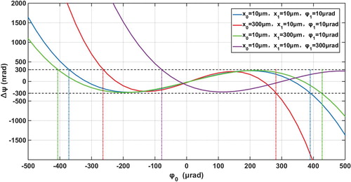
Figure 9 shows the relationship curves with different offset parameters. The blue curve in the picture shows the relationship with all the offset parameters being small. We make it as a reference. Compared with the blue curve, the other curves only change the value of $x_0,{\phi }_1$ and $x_1$ respectively. The following conclusions can be obtained:

1. Increasing the offset length of the flat top beam will reduce the linearity range. This conclusion is same with that in the last two cases.

2. By comparing the purple curve with the blue curve, we can find that with the increasing of the Gaussian beam offset angle, the linearity range within $\pm 300\text{μ}\text{rad}$ decreases. This is mainly due to the change of symmetric centre.

3. Then from the red curve, we can draw the conclusion that increasing the distance between the two optical spots will not reduce the linearity range. Because the intensity gradient of the Gaussian beam decreases from the centre to the edge. However, to guarantee maximum interference efficiency in all the four quadrants, we still need to keep the distance between the Gaussian optical spot and the QPD centre as small as possible.

Figure 9. The relationship between ${\phi }_0$ and $\mathrm{\Delta }\mathrm{\Psi }$ with different parameters. Blue curve: $x_0=10\text{μ}\text{m},x_1=10\text{μ}\text{m},{\phi }_1=10\text{μ}\text{rad}$. Red curve: $x_0=300\text{μ}\text{m},x_1=10\text{μ}\text{m},{\phi }_1=10\text{μ}\text{rad}$. Green curve: $x_0=10\text{μ}\text{m},x_1=300\text{μ}\text{m},{\phi }_1=10\text{μ}\text{rad}$. Purple curve: $x_0=10\text{μ}\text{m},x_1=10\text{μ}\text{m},{\phi }_1=300\text{μ}\text{rad}$.

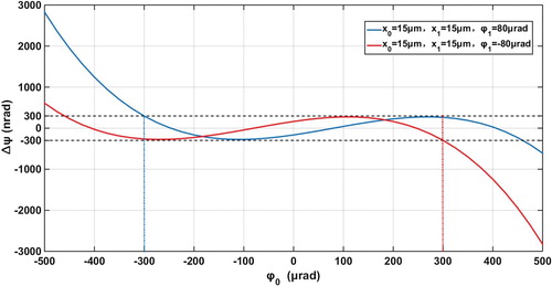
From the conclusions in case 2, we know that $x_0$ should not exceed $15\text{μ}\text{m}$. As mentioned above, the linearity range reduces with the decrease of the distance between the two optical spots. Therefore, we try to find the maximum allowable value of ${\phi }_1$ by taking $x_0=x_1=15\text{μ}\text{m}$. Figure 10 shows the results with ${\phi }_1=\pm 80\text{μ}\text{rad}$. It can be concluded that the absolute value of the Gaussian beam offset angle must be ensured to be smaller than $80\text{μ}\text{rad}$, i.e. $|{\phi }_1|<80\text{μ}\text{rad}$.

Figure 10. The relationship between ${\phi }_0$ and $\mathrm{\Delta }\mathrm{\Psi }$ with $x_0=x_1=15\text{μ}\text{m}$. Blue curve: ${\phi }_1=80\text{μ}\text{rad}$. Red curve: ${\phi }_1=-80\text{μ}\text{rad}$.

3.4. Case 4: the Gaussian beam has an offset in the pitch direction while the flat top beam has an offset in the yaw direction

In this case, the Gaussian beam and the flat top beam deviate in different directions. We suppose that the Gaussian beam has an offset in the pitch direction and the flat top beam deviates in the yaw direction. The offset length of the flat top beam is $x_0$ and the offset angle is ${\phi }_x$, which is also the interested included angle. The offset length of the Gaussian beam is $y_0$ and the offset angle of is ${\phi }_y$. Here, $\mathrm{\Delta }{\phi }_x$ also stands for the absolute measurement error of the included angle. Similarly, the influence of $x_0,y_0$ and ${\phi }_y$ to the linearity range are separately presented in Figure 11.

Figure 11. Blue curve: the relationship between ${\phi }_l$ and $x_0$ with $y_0=10\text{μ}\text{m},{\phi }_y=10\text{μ}\text{rad}$. Red curve: the relationship between ${\phi }_l$ and $y_0$ with $x_0=10\text{μ}\text{m},{\phi }_y=10\text{μ}\text{rad}$. Green curve: the relationship between ${\phi }_l$ and ${\phi }_y$ with $x_0=10\text{μ}\text{m},y_0=10\text{μ}\text{m}$.

We can conclude that:

1. The linearity range reduces with the increase of $x_0$, which is also same with that in the last cases.

2. From the red curve and the green curve, we find that increasing $y_0$ and ${\phi }_y$ will both reduce the linearity range. Because when the flat top beam has an offset in the yaw direction, the difference of wavefront distribution between the left and right quadrants increases with the increase of the Gaussian beam offset in the pitch direction.

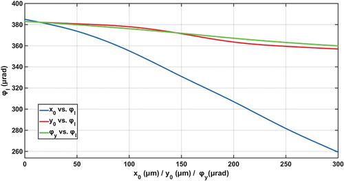
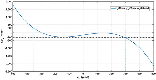
By synthetically considering the offset limits from other cases, we have known that the offset length of the flat top beam should be smaller than $15\text{μ}\text{m}$ while the offset angle of the Gaussian beam should be smaller than $80\text{μ}\text{rad}$. Therefore, we try to find the maximum allowable value of $y_0$ with $x_0=10\text{μ}\text{m},{\phi }_y=80\text{μ}\text{rad}$. Figure 12 shows the numerical result with $y_0=65\text{μ}\text{m}$. It can be seen that the linearity range just meets the demand. As we have concluded that continuing to increase the $y_0$ will reduce the linearity range. Thus, only if $y_0<65\text{μ}\text{m}$, can the requirement of the Taiji be fulfilled.

Figure 12. The relationship between ${\phi }_x$ and $\mathrm{\Delta }{\phi }_x$. Where, $x_0=15\text{μ}\text{m},y_0=15\text{μ}\text{m},{\phi }_y=80\text{μ}\text{rad}$.

If we synthetically consider all the four cases above, the offset parameters have to fulfil the following requirements:

1. The offset length of the Gaussian optical spot from the QPD centre should not exceed $65\text{μ}\text{m}$ while the offset angle of the Gaussian beam should not exceed $80\text{μ}\text{rad}$. These put forward requirement for the ground assembly system.

2. The offset length of the flat top beam should not exceed $15\text{μ}\text{m}$. The precision of the imaging system should guarantee the demand.

It is worth noting that practical situations may be the combination of the four cases. A more complex situation may put forward slightly higher requirements, but it will not differ greatly from the results. Therefore, the requirements above put forward basic demand for the ground assembly system and the imaging system design, which is essential for the Taiji programme.

4. Conclusion

In this paper, we firstly review the development of the DWS technique. As the DWS signal of the Taiji programme is generated by a Gaussian beam and a flat top beam, the linearity performance of such DWS signal is of interest. Then the analytical model of the DWS signal is constructed under a relatively ideal situation and used to qualitatively analyse the linearity performance. For determining the offset range of the beams, a numerical method is subsequently used to analyse four basic practical situations. From the simulations, we draw the conclusion that the linearity range decreases with the increase of the offset angle of Gaussian beam, the as well as the offset length of the flat top beam. The position offset of the Gaussian beam in the orthogonal direction of the flat top beam offset will also decrease the linearity range. Based on the requirement of the Taiji programme, the absolute measurement error of the included angle induced by the non-linear part of the DWS technique should be less than $300\text{nrad}$ within the deviation angle range of $\pm 300\text{μ}\text{rad}$. Combining the requirement and the conclusions above, we obtain the offset range of the two beams. That is, the offset length of the Gaussian optical spot from the QPD centre should not exceed $65\text{μ}\text{m}$, the offset angle of the Gaussian beam should not exceed $80\text{μ}\text{rad}$ and the offset length of the flat top beam should not exceed $15\text{μ}\text{m}$. The method and the results will guide the design of the practical application of the DWS technique in the Taiji programme.

Disclosure statement

No potential conflict of interest was reported by the author(s).

Additional information

Funding

The work is supported by the Strategic Priority Research Program of the Chinese Academy of Science [grant numbers XDA1502070304, XDA1502070902, XDB23030000].

References

- Hu WR, Wu YL. The Taiji Program in Space for gravitational wave physics and the nature of gravity. Nat Sci Rev. 2017;4:685. doi: 10.1093/nsr/nwx116
- Jin G. 2017. Ongoing development of detection of gravitational waves in space in China. Journal of Physics: Conference Series, Volume 840, 11th International LISA Symposium, 5–9 September 2016, Zurich, Switzerland.
- Luo ZR, Bai S, Bian X, et al. Gravitational wave detection by space laser interferometry (in Chinese). Advances in Mechanics. 2013;434:415–447.
- Huang S, Gong XF., Xu P, et al. Gravitational wave detection in space—a new window in astronomy (in Chinese). SCIENTIA SINICA Physica, Mechanica & Astronomica. 2017;47(1):010404. doi: 10.1360/SSPMA2016-00438
- Cirillo F, Gath P. 2008. Control System Design for the Constellation Acquisition Phase of the LISA Mission. Journal of Physics: Conference Series Volume 154, 7th International LISA Symposium 2008, Barcelona, Spain 16-20 June 2008.
- Hyde Y, Maghami PG, Merkowitz SM. Pointing acquisition and performance for the laser interferometry space antenna mission. Classical Quantum Gravity. 2004;21(5). doi: 10.1088/0264-9381/21/5/036
- Jono T., Toyota M, Nakagawa K, et al. 1999. Acquisition, tracking, and pointing systems of OICETS for free space laser communications. Proceedings of the society of photo-optical instrumentation engineers. 3692:41-50 (1999).
- Luo ZR, Wang Q, Mahrdt C., et al. Possible alternative acquisition scheme for the gravity recovery and climate experiment follow-on-type mission. Appl Opt. 2017;56:1495. doi: 10.1364/AO.56.001495
- Hyde TT, Maghami PG. Precision pointing for the laser interferometry space antenna mission. Journal of the Astronautical Sciences. 2003;113:497–508.
- Anderson D. Alignment of resonant optical cavities. Appl Opt. 1984;23(17):2944. doi: 10.1364/AO.23.002944
- Morrison E, Meers BJ, Robertson DI, et al. Experimental demonstration of an automatic alignment system for optical interferometers. Appl Opt. 1994;33(22):5037. doi: 10.1364/AO.33.005037
- Morrison E, Meers BJ, Robertson DI, et al. Automatic alignment of optical interferometers. Appl Opt. 1994;33:5041–5049. doi: 10.1364/AO.33.005041
- Hechenblaikner G. Measurement of the absolute wavefront curvature radius in a heterodyne interferometer. J Opt Soc Am A. 2010;27:2078–2083. doi: 10.1364/JOSAA.27.002078
- Sheard B, Heinzel G, Danzmann K, Shaddock DA, et al. Intersatellite laser ranging instrument for the GRACE follow-on mission. J Geod. 2012;86:1083–1095. doi: 10.1007/s00190-012-0566-3
- Dong YH. 2015. Inter-satellite interferometry: fine pointing and weak-light phase locking techniques for space gravitational wave observatory (in Chinese). [Ph.D. dissertation]. University of Chinese Academy of Sciences.
- Duan HZ, Liang Y-R, Yeh H-C. Analysis of non-linearity in differential wavefront sensing technique. Opt Lett. 2016;41:914. doi: 10.1364/OL.41.000914
- Wanner G, Heinzel G, Kochkina E, et al. Methods for simulating the readout of lengths and angles in laser interferometers with Gaussian beams. Opt Commun. 2012;285:4831–4839. doi: 10.1016/j.optcom.2012.07.123
- Kochkina E, Wanner G, Schmelzer D, et al. Modeling of the general astigmatic Gaussian beam and its propagation through 3D optical systems. Appl Opt. 2013;52:6030. doi: 10.1364/AO.52.006030