A unified dynamic neural field model of goal directed eye movements

ABSTRACT

Primates heavily rely on their visual system, which exploits signals of graded precision based on the eccentricity of the target in the visual field. The interactions with the environment involve actively selecting and focusing on visual targets or regions of interest, instead of contemplating an omnidirectional visual flow. Eye-movements specifically allow foveating targets and track their motion. Once a target is brought within the central visual field, eye-movements are usually classified into catch-up saccades (jumping from one orientation or fixation to another) and smooth pursuit (continuously tracking a target with low velocity). Building on existing dynamic neural field equations, we introduce a novel model that incorporates internal projections to better estimate the current target location (associated to a peak of activity). Such estimate is then used to trigger an eye movement, leading to qualitatively different behaviours depending on the dynamics of the whole oculomotor system: (1) fixational eye-movements due to small variations in the weights of projections when the target is stationary, (2) interceptive and catch-up saccades when peaks build and relax on the neural field, (3) smooth pursuit when the peak stabilises near the centre of the field, the system reaching a fixed point attractor. Learning is nevertheless required for tracking a rapidly moving target, and the proposed model thus replicates recent results in the monkey, in which repeated exercise permits the maintenance of the target within in the central visual field at its current (here-and-now) location, despite the delays involved in transmitting retinal signals to the oculomotor neurons.

KEYWORDS:

• Saccade
• smooth pursuit
• active perception
• dynamic neural field
• sensorimotor contingency

1. Introduction

Dating back to the ideomotor principle from James (1890) in Psychology, the idea that perception and action are tightly intertwined is now widespread and integrated under several different forms in many theories of behavioural and brain sciences. Not only perception guides action, but action also orients perception, both developing and working synergistically for the survival and the autonomy of living beings (Barandiaran, 2016). To act adequately in a dynamic environment, as subjectively perceived based on one's own sensorimotor capabilities, either due to motion in the environment or self-generated movement, synchrony must be maintained despite delays in the sensory, motor and neural pathways of information (Buisson & Quinton, 2010). Anticipation may thus be conceived as a key component to correctly interact with the environment and a fundamental principle underlying the brain activity (Bubic, Von Cramon, & Schubotz, 2010).

Yet, it may actually take on a variety of forms, on a continuum stretching from purely implicit anticipations (relying on past experience to adjust the behaviour to the current and present situation) to explicit ones (with representations of predicted future states), as proposed by Pezzulo (2008). While (more or less abstract) goals and intentions exert an influence down to motor primitives (Rosenbaum, Chapman, Weigelt, Weiss & van der Wel, 2012), it is not trivial to determine how explicit and under which form the anticipatory components are represented. Especially, an internal model predicting the future state of the environment or system may not be required, as interactions with the environment provide the information needed to refine and adjust the course of action, or using Brooks' words (1995): the world is its own best model. The online and implicit differentiation of the various interaction potentialities based on their internal outcomes may be sufficient (Bickhard, 1999). Sensorimotor capabilities, as well as the regularities we learn through interactions, may thus well shape the way the world is perceived. This again goes back to the notion of Umwelt from von Uexküll (1909) and entails a relative conception of space, where space is constructed by individuals and culture, as already proposed by Poincaré (1914) or developed in Piagetian constructivism (1967).

1.1. Visual perception

Focusing on visual perception alone and considering primates (including humans), eye movements can thus be generated to actively sample the external environment, and take part in sensorimotor contingencies (O'Regan & Noë, 2001). Part of the complexity of the relationship between an animal and its environment is thus shared between the sensory and motor aspects of visual perception. Indeed, a non-homogeneous visual stimulation where details are only accessible in the central region of the visual field is sufficient to correctly interact with a natural environment, as long as it is complemented by eye movements and coarse peripheral signals to inform about the outcomes of potential gaze shifts. Furthermore, attention, roughly defined as the active selection and filtering of information based on current skills, knowledge, and context, can be deployed at the overt (e.g. eye movements) and covert (e.g. neural modulation) levels.

Adopting a division classically made when modelling attentional systems (Hopfinger, Buonocore, & Mangun, 2000), this covert deployment of attention results from bottom-up or exogenous factors (e.g. stimulus saliency) as well as top-down or endogenous factors (e.g. stimulus relevance for the task at hand). For instance in Bar (2007), the magnocellular pathway allows making top-down predictions about possible object categories based on coarse information, which is then complemented by the detailed information provided by the slower parvocellular pathway. Yet, in such a dynamical model of visual perception, even when neglecting eye movements, the frontier between the top-down and bottom-up streams is blurred, as the predictions of course depend on expected and known objects, but also directly depend on the sensory stimulation. Additionally, the projections from the prefrontal cortex (object guesses) are often considered as future-oriented in the literature, but actually simply need to get integrated and thus synchronised with the fine grained details when they reach the relevant areas. Directly adding eye movements to the equation, Kietzmann, Geuter, and König (2011) have experimentally demonstrated that simply manipulating the initial locus of visual attention on ambiguous stimuli was sufficient to causally influence the patterns of overt attentional selection, and the recognition of the object's identity. Once again, the differentiation between alternative percepts seems dynamical, rely on expectations about the stimuli, and the sensorimotor interactions are in fact constitutive of visual perception. These three ingredients of visual perception (dynamics, sensorimotricity, and anticipation) are the focus of the current paper, modelling both the covert and overt deployment of visual attention.

Since the exact dynamics of eye movements can itself be quite complex, they have been categorised in different types (see for instance Rolfs, 2009). When looking at static scenes, and at the larger spatial and temporal scales, the eye trajectory is mainly composed of saccades (rapid eye movements) separated by fixations. Nevertheless, these are not independent, and are integrated over time for the coherent perception of extended objects to occur, with possibly predictive aspects (Rolfs, 2015). When looking at the spatio-temporal details, the eyes also continuously perform what is called fixational eye movements, which are a combination of drifts, tremors, and micro-saccades. While the role of saccades to explore the visual environment and foveate stimuli of interest has been previously discussed, micro-saccades may similarly contribute to active vision at a different scale (Hicheur, Zozor, Campagne, & Chauvin, 2013). The neural and functional segregation of the different types of eye movements is debated, and it has been argued that common neural mechanisms may underly saccades and micro-saccades generation (Krauzlis, Goffart, & Hafed, 2017; Otero-Millan, Troncoso, Macknik, Serrano-Pedraza, & Martinez-Conde, 2008).

Now returning to dynamic visual environments, eye-movements toward moving targets are also differentiated, with the interceptive saccades (made first toward the target), the catch-up saccades (made when the lag between the gaze and target directions increases), and the slow pursuit eye movements. To unify the different types of eye-movements with a dynamical perspective, the maintenance of a target within the central visual field can be viewed as a dynamic equilibrium within parallel visuo-oculomotor streams (Goffart, Hafed, & Krauzlis, 2012; Hafed, Goffart, & Krauzlis, 2009). When tracking a moving target, the gaze attempts to synchronise its movement with the motion of the target. The idea that an internal model of the target trajectory would guide the gaze direction (e.g. Daye, Blohm, & Lefèvre, 2014) has recently been questioned (Quinet & Goffart, 2015) because of the failure to define the notion of “trajectory” and the lack of explanation how this notion might be represented in the brain activity.

1.2. Dynamic neural fields

Dynamic neural fields (DNF) are mathematical models based on differential equations, which describe the spatiotemporal evolution of activity (e.g. mean firing rate or membrane potential) in populations of neurons topographically organised within maps. The context of their original development imposed the analytical resolution of the dynamical system, itself requiring strong assumptions on the initial conditions and stimuli characteristics (Amari, 1977; Wilson & Cowan, 1973). Yet, the increasing processing capabilities of computers later allowed simulating the dynamics of such models (Taylor, 1999), at the same time relaxing the constraints and allowing the study of their response to dynamic stimuli.

The core properties of most DNF models is their ability to detect and filter information in the input signal. Targets are detected based on their assumed temporal stability in the signal, as well as their spatial coherence with the lateral connectivity kernel (i.e. the weights of connections between the constituting neurons) (Gepperth, 2014), even in presence of a large amount of noise in the signal. This selection occurs when the system converges to an attractor which encodes the stimulus of interest, under the form of a localised peak of activity (topographical coding). The parameters and nonlinearities in the equation allow implementing qualitatively different mechanisms, from memory formation to sensorimotor coupling. Also, DNF models do not need to be directly plugged on sensory inputs. Therefore, they are not in principle limited to the detection of stimuli defined by a single lateral connectivity profile (for an instance of complex preprocessing to abstract from raw input images, see Maggiani, Bourrasset, Quinton, Berry, & Sérot, 2016). Also, complex transformations and projections can be considered, for instance using a log-polar representation of the visual field (Taouali, Goffart, Alexandre, & Rougier, 2015) or relying on self-organising maps (Lefort, Boniface, & Girau, 2011). While Taouali et al. (2015) provide details on how the DNF approach can account for the encoding of target location in the deep superior colliculus, Gandhi and Katnani (2011) review the different plausible decoding mechanisms from a topologically organised population of neurons, focusing on saccade generation. They compare the “vector summation” and “vector averaging” approaches, the latter being preferred in most of the DNF literature, as well as in the current paper. Regardless of their shared characteristics, computational architectures of visual perception and visual attention based on DNFs come in different flavours, based on the way attractors and transitions between attractors are exploited.

On the one hand, the equation can be tuned to switch between different stable attractors when specific conditions are met. For instance, Sandamirskaya (2014) distinguishes detection and selection instabilities (leading to the selection of one or several targets), working memory instabilities (maintenance of a peak even when the target disappears from the input signal), or reverse detection instability (relaxation of the peak of activity). The rationale and biological inspiration is synthetised in Schöner (2008), and this approach has been successfully applied to model behaviour and to build a wide range of vision and robotic systems (Schöner & Spencer, 2015). This approach is particularly well suited to model discrete behavioural sequences, where specific conditions must be met before turning to the next step (Sandamirskaya & Schöner, 2010). The same applies for sequences of fixations in static environments, with DNF models of the “what” and “where” components of visual perception (Schneegans, Spencer, Schöner, Hwang & Hollingworth, 2014), and of the overt and covert deployment of visual attention (Fix, Rougier, & Alexandre, 2010). However, the delays required to build and relax the peaks makes the modelling of tracking eye movements more complicated.

On the other hand, the robustness of the DNF equations in presence of dynamic input can be directly exploited. For slow target motions (projected within the spatial limits of the neural field), the peak drifts and lags behind the target (Rougier & Vitay, 2006). Nevertheless, the system is able to adapt and converge on a limit cycle attractor, tracking the target. The equation can be modified to further improve the tracking accuracy by biasing the peak dynamics in a given direction, either by making the lateral connectivity kernel asymmetric (Cerda & Girau, 2010), or by adding internal projections of activity to the stimulation (Quinton & Girau, 2011). The latter is chosen and extended in this paper, as we model the tracking of rapidly moving stimuli, as well as the dynamic transitions between the different types of eye-movements.

In the next section, we start by presenting the original DNF model and its extension for tracking a target moving along a continuous trajectory (predictive neural field (PNF)). Then, we extend the system and its dynamics, and introduce the novel ANF model, which incorporates eye-movements to account for the fixation and tracking of targets crossing the visual field. We finally add learning capabilities to the system, to extend its adaptability to trajectories of unknown characteristics. In Section 3, we again incrementally test the different components of the full ANF model, studying the attractors of the associated complex dynamical systems, and evaluating the systems capability to generate different types of eye movements. We then introduce and replicate empirical observations made in monkeys learning to track a target moving along rectilinear trajectories, with dynamic transitions and combinations of saccades and slow pursuit eye movements. We finally close the paper with a short discussion and perspectives.

2. Computational model

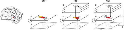
In order to progressively introduce the components of the ANF model, this section starts from the DNF initially proposed by Wilson & Cowan (1973), developed by Amari (1977), and later applied to visual attention directed to moving targets (Rougier & Vitay, 2006). We then introduce the PNF model with a single projection that can bias the dynamics of the neural fields (Quinton & Girau, 2011), then with many projections (Quinton & Girau, 2012), before including eye movements. The increase in model complexity goes hand in hand with extended attentional capabilities, from the detection of fixed targets in the visual field to the generation of tracking eye movements toward a moving target. This progression is illustrated in Figure 1.

Figure 1. Different neural field models used to detect and track a moving target. The original DNF equation may converge on a limit cycle attractor in presence of the target, yet lagging behind it. On the contrary, the projections of the PNF version allows to converge and synchronise with the target motion. If the target crosses the visual field, only the ANF version is able to smoothly track the target, thus mimicking the dynamics of the brain–body-environment system through visuomotor interactions.

2.1. Dynamic neural field

Inspired by neurophysiological studies, including early studies in the visual cortex (Hubel & Wiesel, 1962), DNF are mean-field models of the neural activity when it is observed at the mesoscopic scale. The membrane potential reflects the averaged activity of a large number of topologically organised neurons in response to an input stimulus and its local excitability. Formally, the neural field is represented as a 2D manifold ($\mathit{X}$) in bijection with $[-0.5,0.5{]}^2$, and described by a distribution of potential $\mathit{u}$. The potential at location $\mathit{x}$ and time t is written as $u(\mathit{x},t)$, and the stimulation as $s(\mathit{x},t)$. Adopting the single-layer field equation of lateral inhibition type (Amari, 1977), the dynamics of the potential is described by: (1) $\tau \frac{\mathrm{\partial }u(\mathit{x},t)}{\mathrm{\partial }t}=-u(\mathit{x},t)+c(\mathit{x},t)+s(\mathit{x},t)+h,$(1) where τ is the time constant, h the resting potential and $c(\mathit{x},t)$ the component resulting from lateral interactions over the neural field, defined by: (2) $c(\mathit{x},t)={\int }_{{\mathit{x}}^{\prime }\in \mathit{X}}w({\mathit{x}}^{\prime }-\mathit{x})f\left(u\right({\mathit{x}}^{\prime },t\left)\right)\mathbf{d}{\mathit{x}}^{\prime },$(2) where f is the activation function (in this paper we opted for a rectified linear unit function), while $w(\mathit{x},{\mathit{x}}^{\prime })$ is the lateral connection weight function satisfying Equation (3(3) $w\left(\mathbf{\Delta }\mathit{x}\right)=A_{+}{\mathrm{e}}^{-\parallel \mathbf{\Delta }\mathit{x}{\parallel }^2/{{\sigma }_{+}}^2}-A_{-}{\mathrm{e}}^{-\parallel \mathbf{\Delta }\mathit{x}{\parallel }^2/{{\sigma }_{-}}^2}.$(3) ). (3) $w\left(\mathbf{\Delta }\mathit{x}\right)=A_{+}{\mathrm{e}}^{-\parallel \mathbf{\Delta }\mathit{x}{\parallel }^2/{{\sigma }_{+}}^2}-A_{-}{\mathrm{e}}^{-\parallel \mathbf{\Delta }\mathit{x}{\parallel }^2/{{\sigma }_{-}}^2}.$(3) In a few words, the equation is composed by a relaxation term (driving the local potential to return to its resting level in the absence of stimulation), a lateral interaction term (leading to the selection of one target), and the external stimulation (input driving the neural field dynamics). With adequate stimuli, the resulting selection of a target is proven to occur when the difference of Gaussians in Equation (3(3) $w\left(\mathbf{\Delta }\mathit{x}\right)=A_{+}{\mathrm{e}}^{-\parallel \mathbf{\Delta }\mathit{x}{\parallel }^2/{{\sigma }_{+}}^2}-A_{-}{\mathrm{e}}^{-\parallel \mathbf{\Delta }\mathit{x}{\parallel }^2/{{\sigma }_{-}}^2}.$(3) ) is further constrained to a Mexican hat profile, so that the amplitudes and standard deviations satisfy $A_{+}>A_{-}$ and ${\sigma }_{+}<{\sigma }_{-}$ (Taylor, 1999). In such a case, localised peaks of activity grow on the neural field where stimuli best match the kernel constraints (most often roughly, as for instance with circular visual targets when Gaussian-based kernels are used). Additional constraints can be imposed on the parameters such that one single peak can grow and maintain at a given time, especially through the use of global inhibition with a large ${\sigma }_{-}$ value (see Table 1 for the values adopted throughout this paper). The peak location on the neural field (itself supposedly an estimate of a target location) can be estimated as the centre of mass ${\mathit{x}}_{\mathit{u}}$ of the field activity $\mathit{u}$ (see Equation (4(4) ${\mathit{x}}_{\mathit{u}}=\frac{{\int }_{\mathit{x}\in \mathit{X}}u\left(\mathit{x}\right)\mathit{x}\mathbf{d}\mathit{x}}{{\int }_{\mathit{x}\in \mathit{X}}u\left(\mathit{x}\right)\mathbf{d}\mathit{x}}.$(4) )). (4) ${\mathit{x}}_{\mathit{u}}=\frac{{\int }_{\mathit{x}\in \mathit{X}}u\left(\mathit{x}\right)\mathit{x}\mathbf{d}\mathit{x}}{{\int }_{\mathit{x}\in \mathit{X}}u\left(\mathit{x}\right)\mathbf{d}\mathit{x}}.$(4) Equation (1(1) $\tau \frac{\mathrm{\partial }u(\mathit{x},t)}{\mathrm{\partial }t}=-u(\mathit{x},t)+c(\mathit{x},t)+s(\mathit{x},t)+h,$(1) ) can be simplified by relying on a map-based notation for the different components, thus assimilating $u(\mathit{x},t)$ to a $\mathit{X}\to [0,1]$ map written as $\mathit{u}$, thus leading to the following equation: (5) $\tau \frac{\mathrm{\partial }\mathit{u}\left(t\right)}{\mathrm{\partial }t}=-\mathit{u}\left(t\right)+\mathit{c}\left(t\right)+\mathit{s}\left(t\right)+h.$(5) Turning to the computational implementation, we rely on an explicit Euler schema to simulate the dynamics. Time is thus discretised with an interval $\mathrm{d}t$ between two estimations, and a square regular lattice discretisation is used for space (allowing a matrix-based implementation). The continuous version in Equation (5(5) $\tau \frac{\mathrm{\partial }\mathit{u}\left(t\right)}{\mathrm{\partial }t}=-\mathit{u}\left(t\right)+\mathit{c}\left(t\right)+\mathit{s}\left(t\right)+h.$(5) ) becomes: (6) $\mathbf{u}\left(t\right)=\left(1-\frac{\mathrm{d}t}{\tau }\right)\mathbf{u}(t-\mathrm{d}t)+\frac{\mathrm{d}t}{\tau }(\mathbf{w}\ast f(\mathbf{u}(t-\mathrm{d}t))+\mathbf{s}(t\left)\right)$(6) with $\mathbf{u}$, $\mathbf{s}$ and $\mathbf{w}$ being the matrix equivalents for variables and functions $\mathit{u}$, $\mathit{s}$ and w. To the exception of a few lines of work (e.g. Cerda & Girau, 2010), the kernel function w is usually isotropic (as in Equation (3(3) $w\left(\mathbf{\Delta }\mathit{x}\right)=A_{+}{\mathrm{e}}^{-\parallel \mathbf{\Delta }\mathit{x}{\parallel }^2/{{\sigma }_{+}}^2}-A_{-}{\mathrm{e}}^{-\parallel \mathbf{\Delta }\mathit{x}{\parallel }^2/{{\sigma }_{-}}^2}.$(3) )). The absence of $\mathbf{x}$ in this formulation reflects the fact that a peak of maximal amplitude only grows in presence of a stationary localised stimulus, and aligns with it. In response to a stimulus which is not aligned with the peak of activity, the properties of the DNF equation and lateral connectivity kernel lead to an averaging of the stimulus projection, and thus its location, at time t (with weight $\mathrm{d}t/\tau$) with the reentrant feedback of the neural field, with a peak that emerged up to $t-\mathrm{d}t$ (with weight $1-\mathrm{d}t/\tau$). When combining different sources of activity to drive the field dynamics, this averaging property has been widely exploited in the literature, for instance to model saccadic motor planning (Kopecz & Schöner, 1995) in the context of active vision, or multimodal integration models able to replicate the McGurk effect (Lefort et al., 2011). Yet in the context of tracking a moving target, this property implies that the peak necessarily lags behind the input stimulus with the standard equation. The amount of lag depends on the $\mathrm{d}t$ and τ parameters, as well as on the stimulus dynamics (e.g. the stimulus instantaneous velocity, that is noted ${\mathit{v}}_{\mathit{s}}$ in the rest of the paper). Nevertheless, this lag cannot be fully cancelled with an isotropic kernel (as illustrated in the DNF part of Figure 1). Additionally, increasing the $\mathrm{d}t/\tau$ ratio enhances the reactivity of the neural field, yet simultaneously reduces its relaxation time and filtering efficiency, two key components of computational models of attention.

Table 1. Parameters and variables of the neural field model.

Group of parameters	Description	Symbol	Value/space
Visual field
	Visual field space	$\mathit{X}$	$[-0.5,0.5{]}^2$
	Coordinates within the field	$\mathit{x}$	$\in \mathit{X}$
	Field coordinates (world reference frame)	${\mathit{x}}_{\mathit{f}}$	$\in {\mathbb{R}}^2$
Neural field equation/potential		$\mathit{u}$	$\mathit{X}\to [0,1]$
	Time constant	τ	0.2
	Resting potential	h	0
	Firing/activation function (ReLU)	f	$\mathbb{R}\to {\mathbb{R}}^{+}$
	Stimulation/projection coefficient	α	0.5
	Focus coordinates (peak centre)	${\mathit{x}}_{\mathit{u}}$	$\in \mathit{X}$
Lateral connectivity kernel		$\mathit{w}$	$\mathit{X}\to [-1,1]$
	Excitatory amplitude	$A_{+}$	0.06
	Excitatory range (sd)	${\sigma }_{+}$	0.1
	Inhibitory amplitude	$A_{-}$	0.03
	Excitatory range (sd)	${\sigma }_{-}$	1.0
Gaussian stimulus		$\mathit{s}$	$\mathit{X}\to [0,1]$
	Stimulation amplitude	$A_s$	$\in \{0,1\}$
	Stimulation range (sd)	${\sigma }_s$	0.1
	Stimulus noise (white)	$\mathit{ϵ}$	$\mathit{X}\to \mathbb{R}$
	Noise amplitude (sd)	${\sigma }_{ϵ}$	0.2
	Stimulus velocity	${\mathit{v}}_{\mathit{s}}$	$\in [-3,3{]}^2$
	Stimulus location (field reference frame)	${\mathit{x}}_{\mathit{s}}$	$\in \mathit{X}$
	Stimulus location (world reference frame)	${\hat{\mathit{x}}}_{\mathit{s}}$	$\in {\mathbb{R}}^2$
Projection(s)		${\mathit{p}}_{\mathit{k}}$	$\mathit{X}\to [-1,1]$
	Projection weight (validity)	$w_k$	$\in [0,1]$
	Projection “velocity”	${\mathit{v}}_{\mathit{k}}$	$\in [-5,5{]}^2$
Eye movement
	Motor space	$\mathit{A}$	$[-1,1{]}^2$
	Motor command	$\mathit{a}$	$\mathit{A}$
	Induced spatial displacement	${\mathit{x}}_{\mathit{a}}$	$[-1,1{]}^2$
	Associated projection	${\mathit{p}}_{\mathit{a}}$	$\mathit{X}\to [-1,1]$
	Activation threshold	$u_a$	0.4
Discretisation/dynamics
	Time	t	$\in \mathbb{R}$
	Time step	$\mathrm{d}t$	0.05
	Spatial resolution	n	51

2.2. Predictive neural field

To synchronise the peak of activity with the input stimulus, as in presence of a rapidly moving target, the reactivity of the field can be enhanced at the cost of robustness to sensory noise (by adjusting the equation parameters). Yet, to reduce the tracking lag without relying on the trade-off between reactivity and stability, the original equation can be modified in two ways: by using asymmetric kernels, or by turning the stimulation term into a combination of both the sensory signal and an internal model (corresponding roughly to a memory trace) of the stimulus dynamics. Asymmetric kernels have been used in Cerda and Girau (2010) with different motions requiring different kernels (${\mathbf{w}}_k$). To discriminate between complex motions, the kernels become location dependent, and iterations over many time steps are required. A set of independent neural fields have been previously used to cover the range of expected motions, but kernels could also be dynamically weighted and combined to reflect the probability of the expected motions (model) to fit the actual dynamics (observation). Here, in order to facilitate transitions between trajectories, and to permit their combination into novel trajectories with which the system can synchronise, we rather proceeded on the decomposition of the stimulation term (Quinton and Girau, 2011, 2012). From a neural perspective, these approaches may all break down to adjusting synaptic weights on the long term (to adapt to new forms of motion), and synaptic gating on the short term (to exploit the repertoire of expected motion). Yet, the modularity and the precise dynamics of these approaches differ because of the way the information is distributed and injected in the equations. In this paper, the term $\mathit{s}\left(t\right)$ in Equation (5(5) $\tau \frac{\mathrm{\partial }\mathit{u}\left(t\right)}{\mathrm{\partial }t}=-\mathit{u}\left(t\right)+\mathit{c}\left(t\right)+\mathit{s}\left(t\right)+h.$(5) ) is thus replaced by $\hat{\mathit{s}}\left(t\right)$, defined as: (7) $\hat{\mathit{s}}\left(t\right)=\alpha \mathit{p}\left(t\right)+(1-\alpha )\mathit{s}\left(t\right),$(7) where α weights the external stimulation $\mathit{s}\left(t\right)$ and an internal projection $\mathit{p}\left(t\right)$. This projection corresponds to the activity required to cancel the lag of the neural field for a specific hypothetically observed trajectory, by exciting the field in the direction of the motion, ahead of the current peak location, and inhibiting the field behind the peak. While it may seem counter-intuitive to make such a substitution, incoming signals for both components may arrive from distal neural areas, only with some of them more directly connected to the actual physical stimulus (in terms of temporality or similarity). Their origin cannot be accessed in the current model, and due to their symmetrical roles in the equation, they cannot be differentiated at the level of the neural field. Alternatively, adopting a division classically made when modelling attentional systems (Hopfinger et al., 2000), these components may respectively be described as bottom-up and top-down, while the voluntary nature of such influences is beyond the scope of the current paper. The component $\mathit{p}\left(t\right)$ is further decomposed in Equation (8(8) $\mathit{p}\left(t\right)=\frac{\sum _k{w}_k\left(t\right){\mathit{p}}_{\mathit{k}}\left(t\right)}{\sum _k{w}_k\left(t\right)}.$(8) ), but in this paper, it is exclusively computed from the field potential $u\left(t\right)$. A null α restores the original dynamics, while an α of 1 leads to a closed-loop dynamics disconnected from the external stimulation. An α in $]0,.5]$ guarantees that the dynamics is not driven by the internal projections, but by the actual external dynamics. (8) $\mathit{p}\left(t\right)=\frac{\sum _k{w}_k\left(t\right){\mathit{p}}_{\mathit{k}}\left(t\right)}{\sum _k{w}_k\left(t\right)}.$(8) The term $\mathit{p}$ is expressed as a combination of individual projections $\left\{{\mathit{p}}_{\mathit{k}}\right\}$, which correspond to distinct dynamics observed in different contexts (e.g. different trajectories adopted by different targets). The set $\left\{{\mathit{p}}_{\mathit{k}}\right\}$ might as well define a basis of projections, learned from the statistics of observed trajectories, and which can be combined, endowing the system with the ability to adapt to more complex dynamics. Any complex and extended trajectory can for instance be approximated by a smooth interpolation over a sequence of projections, each projection corresponding to a simpler local target motion (temporal weighting). Each unique local projection can also result from a combination of a limited set of projections (spatial weighting), corresponding to target motions with specific directions and speeds. These population coding properties within the neural field have been described elsewhere (for independent projections see Quinton and Girau (2011); for combinations within a set of projections see the supplemental material from Quinton and Girau (2012)). The weight $w_k$ of each projection changes with time; it is not to be confused with the fixed connection weights w in the original DNF equation. While the former reflects the adequacy of projection ${\mathit{p}}_{\mathit{k}}$ with the currently observed dynamics and thus translates the competition between projections in mathematical terms, the latter guarantees the competition between possible locations for the peak growth (as introduced in Section 2.1). Although the details on the updating of the weight $w_k$ are not required at this point, it can simply be considered as a similarity measure between the actual neural field activity $\mathit{u}$ and the expected activity (approximated by $\mathit{p}$). Basically, the associated dissimilarity may be a norm based on point to point differences at the map level, continuously updated during the simulation.

Again, the normalisation in Equation (8(8) $\mathit{p}\left(t\right)=\frac{\sum _k{w}_k\left(t\right){\mathit{p}}_{\mathit{k}}\left(t\right)}{\sum _k{w}_k\left(t\right)}.$(8) ) guarantees the influence of the overall internal projection of activity on the neural field will not have primacy over the input, since the number of projections on which it is based may vary (e.g. due to learning effects of repeated exercise and the variability of observed trajectories, therefore not reducible to a single projection). Simultaneously high weights for two projections should reflect their similarity, with the neural field averaging their activity. On the contrary, two equally active yet clearly distinct projections will not both lead to a large similarity with the neural field activity (where at most a single peak is present), and a bifurcation will necessarily occur in their weights. Although other aggregation functions could be considered in replacement of the simple linear combination of the projections (Equation (8(8) $\mathit{p}\left(t\right)=\frac{\sum _k{w}_k\left(t\right){\mathit{p}}_{\mathit{k}}\left(t\right)}{\sum _k{w}_k\left(t\right)}.$(8) )), the neural field dynamics attenuates or nullifies the influence of projections with relatively small weights through lateral interactions. In these three instances, we indirectly exploit the usual selection (for distant stimuli), averaging (for nearby target stimuli and their overlapping field activations) and robustness (for distributed noisy stimulations) properties of the DNF.

As previously introduced, projections may be defined for any type of target trajectory, but in this paper, we will limit their scope to rectilinear motions with a constant speed. Stimuli adopting such trajectories will be used in the evaluation section to test the robustness of the model and replicate experimental data. Also, and as any trajectory can be approximated with an arbitrary precision by a set of local linear motions, the aforementioned restriction should be of no consequence for the expressive power of the model. Each projection can be defined as a geometric transformation of the field potential $\mathit{u}\left(t\right)$, a transformation that may itself depend upon time, but will be limited here to a fixed translation (which may be combined to approximate more complex trajectories). We thus define: (9) ${\mathit{p}}_{\mathit{k}}(\mathit{x},t)=u(\mathit{x}-\mathbf{\Delta }\mathit{x},t-\mathrm{\Delta }t),$(9) which corresponds to a shift of $\mathbf{\Delta }\mathit{x}$ performed in $\mathrm{\Delta }t$. From a neural perspective, we do not want to consider delay differential equations, in which the continuous propagation of activity over the neural field would lead to infinitesimal shifts when considering decreasing periods of time. If we consider the internal projections to be the result of back-and-forth projections between neural fields or neural areas, there will be a minimal delay $\mathrm{\Delta }t\gg 0$ before any signal generated from the neural field activity returns to it. Then, for any fixed “projection velocity” ${\mathit{v}}_{\mathit{k}}$, the equivalent shift must be set, or adjusted, so that $\mathbf{\Delta }\mathit{x}={\mathit{v}}_{\mathit{k}}\mathrm{\Delta }t$. The delay $\mathrm{\Delta }t$ may of course depend on the connectivity, thus also on the location within the neural field, but will be considered constant in the current paper with any loss in expressiveness. Also, and to return the mathematics of the system, a large enough delay is required to discriminate between projections and allow bifurcations in the system (through weights $w_k$), since differences will become negligible when the delay approaches zero (in terms of signal-to-noise ratio). Reversely, a too large delay leads to projections no more interacting with a pre-existing peak of activity (through the connectivity kernel of limited excitatory width), and thus has a reduced impact on the neural field dynamics. Practically, there is no need for such projection to be defined for any $\mathit{x}\in \mathit{X}$, as they simply need to sufficiently cover the neural field, which embeds continuity and smooth out irregularities (with increased weights $w_k$ possibly compensating for the reduction of effect due to sparsity). Instead of considering projections as transformations of the entire neural field activity, we can indeed decompose projections as local stimulations, responding to distant and past activity on the field. For each location targeted by a projection, we can define an input receptive field on the neural field, reacting to the presence of a peak of activity. Such local projections then define a set of tuning curves (Zhang & Sejnowski, 1999) and the system dynamics will remain roughly the same, as long as the receptive fields overlap sufficiently.

When turning to the computational implementation of Equation (9(9) ${\mathit{p}}_{\mathit{k}}(\mathit{x},t)=u(\mathit{x}-\mathbf{\Delta }\mathit{x},t-\mathrm{\Delta }t),$(9) ) , we want to respect both the spatial and temporal discretisation of the neural field. We therefore synchronise the updates with $\mathrm{\Delta }t=n\times dt$ ($n\in {\mathbb{N}}^{\ast }$). Additionally, as long as both $\mathrm{d}t$ and n are neither too small (with birfurcation issues) nor too large (with lateral interaction issues), n remains a free parameter of the system. It is here arbitrarily set to 1, which gives the following equation when also introducing a second term to facilitate the relaxation of activity at the previous (peak) location: (10) ${\mathit{p}}_{\mathit{k}}(\mathit{x},t)=u(\mathit{x}-{\mathit{v}}_{\mathit{k}}\mathrm{d}t,t-\mathrm{d}t)-u(\mathit{x},t-\mathrm{d}t).$(10) With this equation, a peak centred on $\mathit{x}$ at time $t-\mathrm{d}t$ should move to the location $\mathit{x}+{\mathit{v}}_{\mathit{s}}\mathrm{d}t$ at time t. At this stage, the reader might wonder about the relationship between the velocity of the peak ${\mathit{v}}_{\mathit{u}}$ (derivative of ${\mathit{x}}_{\mathit{u}}$), the projection velocity ${\mathit{v}}_{\mathit{k}}$ and the instantaneous velocity of the tracked stimulus ${\mathit{v}}_{\mathit{s}}$ (of course unknown and not explicitly computed within the neural field model). If all velocities are expressed in the same coordinate system, we should expect the peak to move at speed ${\mathit{v}}_{\mathit{u}}={\mathit{v}}_{\mathit{s}}$, ideally in perfect synchrony with the stimulus (i.e. with no lag). The naive approach is to consider that a single projection ${\mathit{p}}_{{\mathit{k}}_{\mathbf{0}}}$ from Equation (8(8) $\mathit{p}\left(t\right)=\frac{\sum _k{w}_k\left(t\right){\mathit{p}}_{\mathit{k}}\left(t\right)}{\sum _k{w}_k\left(t\right)}.$(8) ) should be active (i.e. $w_k\ne 0⟺k=k_0$), or that projections should combine into a single equivalent projection ${\mathit{p}}_{\mathit{k}}$ associated with ${\mathit{v}}_{\mathit{k}}={\mathit{v}}_{\mathit{s}}$. However, the dynamics of the peak (including its location and shape) makes the picture a bit more complicated. For instance, the projection only contributes to the updated activity with coefficient $\alpha \mathrm{d}t/\tau$ , so that we need to choose ${\mathit{v}}_{\mathit{k}}=\gamma {\mathit{v}}_{\mathit{s}}$ with $\gamma >1$ in order to compensate for the peak inertia (which is a direct consequence of the original equation). A reformulation and approximation of the problem would thus lead to the following definition to optimally synchronise with the target motion : (11) ${\mathit{p}}_{\mathit{k}}(\mathit{x},t)=u(\mathit{x}-\gamma {\mathit{v}}_{\mathit{s}}\mathrm{d}t,t-\mathrm{d}t)-u(\mathit{x},t-\mathrm{d}t).$(11) Further details and demonstration on this speed overestimation are provided in Quinton and Girau (2011), and are illustrated in the PNF (fast) part of Figure 2. In practice, a simple model as expressed in Equation (11(11) ${\mathit{p}}_{\mathit{k}}(\mathit{x},t)=u(\mathit{x}-\gamma {\mathit{v}}_{\mathit{s}}\mathrm{d}t,t-\mathrm{d}t)-u(\mathit{x},t-\mathrm{d}t).$(11) ) cannot account for the complex dynamics of the neural field, and learning is required to correctly estimate the map between $\mathit{u}$ and $\mathit{p}$ for any fixed target velocity ${\mathit{v}}_{\mathit{s}}$. It is unrealistic to assume targets should follow a trajectory with stable characteristics on a sufficiently large time window $[0,T]$, so that a projection ${\mathit{p}}_{\mathit{k}}$ could be independently learned to synchronise the peak and target dynamics. In practice, the set of weights $w_k$ should be also learned as functions of the neural field state, testing if the projection facilitates the synchronisation with the target, for which the actual location, velocity, or even presence are unknown. While a form of predictive coding could be considered, the crucial problem remains that the projection velocity ${\mathit{v}}_{\mathit{k}}$ and the peak velocity used to test the prediction are different, and related by a complicated function that also depends on most of the neural field parameters. When combining all these factors, the problem is far from being trivial to solve through unsupervised learning. These difficulties will not be directly addressed in this paper, and are simply highlighted as they will partly be dissolved when turning to the ANF model in the next section. We will therefore rely on Equation (10(10) ${\mathit{p}}_{\mathit{k}}(\mathit{x},t)=u(\mathit{x}-{\mathit{v}}_{\mathit{k}}\mathrm{d}t,t-\mathrm{d}t)-u(\mathit{x},t-\mathrm{d}t).$(10) ) in the rest of the paper.

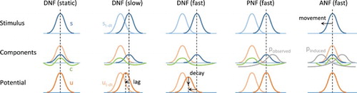
Figure 2. Illustration of the neural field model dynamics and equation components. For each model, stimulation at time $t-\mathrm{d}t$ (light colour on first row) and t (dark colour on first row), field activity from $t-\mathrm{d}t$ (light colour on third row) and resulting at t (dark colour on third row), as well as the competition component (negative activity on second row), are represented. Internal input projections corresponding to expected trajectories are also shown for the PNF and ANF models. With a moving stimulus, the DNF model is not able to converge to a stable peak of maximal activity, the peak lagging behind the target and/or decaying. The projection of activity in the PNF model simply compensates for the inertia of the equation and synchronises with the target trajectory (if the implicit expectation and observation match). The ANF model additionally includes a projection due to the eye movement, thus cancelling the drifting effect of the projection when the target image is kept within the central visual field.

With target motions remaining within the limits of the visual field, the aim of the PNF model is to extend the covert attentional capabilities of classical DNFs. As described in Quinton and Girau (2011), the field potential $\mathit{u}$ may converge to a limit cycle in presence of a periodic target trajectory, even when the stimulus speed is increased, and without the alternation of decaying and building peaks observed with the original equation. That is, the peak velocity ${\mathit{v}}_{\mathit{u}}$ on the neural field will be equal to the stimulus velocity ${\mathit{v}}_{\mathit{s}}$. Also, robustness to noise and distractors is increased, since the target is now characterised by its spatiotemporal dynamics and not only by its shape compatibility with the kernel profile. Thus, and contrary to Rougier and Vitay (2006) for instance, distractors can have the exact same spatial characteristics and be visible during the entire simulation, but simply adopt a non-expected trajectory. It is therefore possible to discriminate and interpolate between trajectories in a nonlinear fashion, thanks to the feedback loop of projections validity ($w_k$) in the PNF equation (Quinton & Girau, 2012). Finally and as a consequence, the system becomes also robust to the temporary disappearance of the target (e.g. due to occlusion). In such a case, the peak decays in absence of stimulation, but initially keeps tracking the stimulus at its current (here and now) location. Indeed, the inertia induced by the original equation remains effective, with the peak and projection positively exciting each other (a high $w_k$ leading to a larger peak amplitude and vice versa). Nevertheless, this behaviour is short-lived (a few hundred milliseconds with current parameters) since the input and thus the weight of other projections rapidly regain a significant impact (because of $\alpha <.5$ in Equation (7(7) $\hat{\mathit{s}}\left(t\right)=\alpha \mathit{p}\left(t\right)+(1-\alpha )\mathit{s}\left(t\right),$(7) )).

In the context of this paper, the most striking feature of the PNF model is that the projection of activity ${\mathit{p}}_{\mathit{k}}$ on the neural field is actually not a prediction of the present state $\mathit{u}\left(t\right)$. Prediction usually supposes a projection into the future, and while the projection ${\mathit{p}}_{\mathit{k}}$ is indeed built based on the state of the field activity at time $t-\mathrm{\Delta }t$ (and thus oriented toward the future), it only influences the dynamics and effectively gets projected onto the field at time t (thus in the present, if we consider the external world to be setting the time reference). More importantly, while the field potential $\mathit{u}(t-\mathrm{\Delta }t)$ can be conceived as the input to generate an internal expected or experienced trajectory, the projection ${\mathit{p}}_{\mathit{k}}$ generated in return is a form of internal action on the neural field, which alters its dynamics. The projection term thus is not required to be in direct relation with the external stimulation $\mathit{s}$, but simply allows maximising the synchrony between the system and stimulus dynamics, that is, minimising the distance between ${\mathit{x}}_{\mathit{s}}$ (actual stimulus location) and ${\mathit{x}}_{\mathit{u}}$ (estimated location). In other words, we should not expect the weight $w_k$ (somehow the confidence in the projection ability to facilitate synchrony) to be correctly estimated based on the difference between the projection ${\mathit{p}}_{\mathit{k}}$ and the present field state $\mathit{u}\left(t\right)$ or stimulation $\mathit{s}\left(t\right)$. Even though they end up being combined in the neural field space $\mathit{X}$, they correspond to qualitatively different concepts; if $\mathit{u}(t-\mathrm{\Delta }t)$ provides part of the context, ${\mathit{p}}_{\mathit{k}}$ is the action, and $\mathit{u}\left(t\right)$ the outcome. At this point, two limitations lead to the development of the ANF model: 1) Such projections require to learn or approximate the relation between ${\mathit{v}}_{\mathit{s}}$, ${\mathit{v}}_{\mathit{u}}$ and ${\mathit{v}}_{\mathit{k}}$ for any location on the field. 2) The model is limited to covert attention (with the absence of eye movements), as a target leaving the visual field will be lost.

While a heterogeneous field of view (e.g. characterising the retina with a central macula and fovea) could be viewed as a complicating factor for the above issues, it is actually a solution to the problem when one considers the generation of eye movements. Foveating a target indeed facilitates its pursuit by increasing the neural resources for processing the motion signals, and at the same time hinder and make unnecessary the learning of stimuli dynamics for all locations of the visual field. Learning to foveate the target and keep it in the central visual field will reduce the problem to processing the motion signals and characterise the dynamics of the input stimulus. Also pointing in such direction, a model of target position encoding in the superior colliculus has been recently proposed in Taouali et al. (2015), demonstrating that apparently complex foveation performance can be accounted for by dynamical properties of neural field and retinotopic stimulation (using a log-polar representation of the visual field).

2.3. Active neural field

The new active neural field (ANF) model proposed in this paper extends the previous models by introducing eye movements, complementing the covert attentional deployment (Quinton & Girau, 2011), with overt shifts of attention. The system thus aims at reaching a fixed point attractor when a target is stabilised in the visual field , while performing eye movements synchronised with the motion of the target. Action is now not only performed through projections to the neural field, but also through a physical movement of the simulated eyes. To simplify the model, we will here rely on a Cartesian coordinate system and a homogeneous resolution over the visual field, although some advantages of turning to a more realistic retinal model will be developed in the final discussion. While such increments to the model may seem limited in terms of equations, they drastically extend the capabilities of the system, change the characterisation of the attractors of the associated dynamical system, as well as the dimensionality and structure of the learning space. The following sections therefore focus on these aspects.

Physical actions are initiated once an activity threshold $u_a$ is reached on the neural field, reflecting the detection of a target. With a sufficiently high value for $u_a$, the maximal activity of the neural field ($\parallel u{\parallel }_{max}$) should indeed correspond to the centre of an existing or forming peak, and the field activity can be directly exploited to orient the simulated eye toward the estimated target location. An alternative way to achieve the same result, often adopted in the DNF literature, is to adjust the resting level h from the original DNF equation, while setting $u_a=0$. A peak maintained above the threshold will continuously feed the movement generators, but such a peak can hardly be maintained away from the neural field centre (details will be provided with the analysis of the system dynamics in the result section). This threshold reflects a kind of “cost” for moving the eyes (energy, time, blur), since its absence would lead to continuous movements of possibly large amplitude. Indeed, in absence of an already high peak, the estimated (peak) location (following Equation (4(4) ${\mathit{x}}_{\mathit{u}}=\frac{{\int }_{\mathit{x}\in \mathit{X}}u\left(\mathit{x}\right)\mathit{x}\mathbf{d}\mathit{x}}{{\int }_{\mathit{x}\in \mathit{X}}u\left(\mathit{x}\right)\mathbf{d}\mathit{x}}.$(4) )) can be subject to quick variations, simply because of small variations of the potential $\mathit{u}$ induced by noise in the input signal. The activity threshold $u_a$ is set to $.4$ in this paper, but it is dependent on the neural field parameters.

All actions in this system are aimed at bringing the target within the central visual field (generating an associated peak at the centre of the neural field), consequently limiting the parameter space to explore for learning. Actions can thus be represented as a map $\mathit{a}$ from the field activity to the motor system. In turn, the action $\mathit{a}$ leads to an apparent movement on the field of view $-{\mathit{x}}_{\mathit{a}}$, which is approximately equal to $-{\mathit{x}}_{\mathit{u}}$ (thus the movement simply zeroes out the eccentricity of the target at its current estimated location). In experimental data, both smooth pursuit and saccadic eye movements correspond to continuous movements, but with qualitatively different speed profiles. Although testing the fit between the generated saccade profiles and those observed in experimental settings is meaningless here, due to the simplistic implementation of oculomotor control, the apparent discontinuity of the movement in the model is merely due to the temporal discretisation of the differential equations. As a proof of concept model and for simplicity and explanatory purpose, saccades will always be performed over one time step in the current model, regardless of their amplitude. As a consequence, and for such movements to remain biologically plausible, a lower limit to $\mathrm{d}t$ is imposed for the simulation (this is already guaranteed when considering the projection delay $\mathrm{\Delta }t$, as described in previous section).

To refine the previous notations for a controllable field of view, let ${\mathit{x}}_{\mathit{f}}$ be the centre of the field of view in the world reference frame. Assuming Cartesian coordinates, and applying the adequate action $\mathit{a}\left(\mathit{u}\right(t\left)\right)$ to centre the currently focused target should lead to the following changes at t+dt: (12a) $\begin{array}{rl}{\mathit{x}}_{\mathit{f}}(t+dt)& ={\mathit{x}}_{\mathit{f}}\left(t\right)+{\mathit{x}}_{\mathit{a}}\left(\mathit{a}\right(\mathit{u}\left(t\right))={\mathit{x}}_{\mathit{f}}(t)+{\mathit{x}}_{\mathit{u}}(t)+\eta ,\end{array}$(12a) (12b) $\begin{array}{rl}{\mathit{x}}_{\mathit{s}}(t+dt)& ={\mathit{x}}_{\mathit{s}}\left(t\right)-{\mathit{x}}_{\mathit{a}}\left(\mathit{a}\right(\mathit{u}\left(t\right))={\mathit{x}}_{\mathit{s}}(t)-{\mathit{x}}_{\mathit{u}}(t)-\eta ,\end{array}$(12b) where η is an error term that is minimised through learning to allow perfectly centred fixations of targets. While the action map $\mathit{a}$ and the sensory consequence ${\mathit{x}}_{\mathit{a}}$ of performing the action can both be easily given here (starting from Equation (4(4) ${\mathit{x}}_{\mathit{u}}=\frac{{\int }_{\mathit{x}\in \mathit{X}}u\left(\mathit{x}\right)\mathit{x}\mathbf{d}\mathit{x}}{{\int }_{\mathit{x}\in \mathit{X}}u\left(\mathit{x}\right)\mathbf{d}\mathit{x}}.$(4) ) for the extraction of the peak location), such transformations can be learned in DNF models. For instance, Bell, Storck, and Sandamirskaya (2014) focus on saccade generation and learning of the coupling between target location encoding and motor commands. Even with the simple Cartesian coordinate systems used here, the world and visual field reference frames must be clearly distinguished, or equivalently the apparent location ${\mathit{x}}_{\mathit{s}}$ of the stimulus from its physical location in the world reference frame, defined by ${\hat{\mathit{x}}}_{\mathit{s}}={\mathit{x}}_{\mathit{f}}+{\mathit{x}}_{\mathit{s}}$. With the emergence of a peak in response to a static target, we get ${\mathit{x}}_{\mathit{u}}\left(t\right)\approx {\mathit{x}}_{\mathit{s}}\left(t\right)$ before the saccade is initiated, and thus ${\mathit{x}}_{\mathit{s}}(t+\mathrm{d}t)\approx 0$. The learning of eye movements can be made independent to that of the projections dealing with observed movements, as the structure of the visual space can be acquired when looking at or away from static targets (or those adopting slow movements for which the original DNF dynamics is sufficient). Because of the inertia in the original equation, projections can also be associated to eye movements, facilitating the relaxation of the eccentric peak and the emergence of a new (theoretically central) peak of activity. The associated projection of activity can thus be defined by: (13) $p_a(\mathit{x},t)=u(\mathit{x}-{\mathit{x}}_{\mathit{a}}(\mathit{a}\left(\mathit{u}\right(t-\mathrm{d}t\left)\right)),t-\mathrm{d}t)-u(\mathit{x},t-\mathrm{d}t).$(13)

The entire neural field architecture for the ANF model is represented in Figure 3. When a peak of activity grows on the neural field in response to a target, saccades, once performed, systematically induce stimulations near the centre of the visual field. For the previously introduced PNFs, the prediction ${\hat{\mathit{p}}}_{\mathit{k}}$ and projection ${\mathit{p}}_{\mathit{k}}$ in Equations (10(10) ${\mathit{p}}_{\mathit{k}}(\mathit{x},t)=u(\mathit{x}-{\mathit{v}}_{\mathit{k}}\mathrm{d}t,t-\mathrm{d}t)-u(\mathit{x},t-\mathrm{d}t).$(10) ) and (11(11) ${\mathit{p}}_{\mathit{k}}(\mathit{x},t)=u(\mathit{x}-\gamma {\mathit{v}}_{\mathit{s}}\mathrm{d}t,t-\mathrm{d}t)-u(\mathit{x},t-\mathrm{d}t).$(11) ) will not be correct or at least optimal anymore, as they are designed for target motions with constant velocities. Yet, if a moving target leads to a peak away from the centre, the projection associated with the expected motion (${\mathit{p}}_{\mathit{k}}$) will not be compatible with the post-saccadic central stimulation, while both the inhibitory component from the ${\mathit{p}}_{\mathit{k}}$ and ${\mathit{p}}_{\mathit{a}}$ components will facilitate the relaxation of the earlier peak and thus a refocus on new apparent location of the target. If the peak appears near the centre of the visual field, with the target moving away from the centre (i.e. with the eye movement lagging behind the target) , projections ${\mathit{p}}_{\mathit{a}}$ and ${\mathit{p}}_{\mathit{k}}$ will have opposite effects on the dynamics. For a projection in adequation with the stimulus velocity, ${\mathit{p}}_{\mathit{a}}$ and ${\mathit{p}}_{\mathit{k}}$ will cancel out and stabilise the peak when the continuous eye movements (induced motion ${\mathit{x}}_{\mathit{a}}$ at each iteration) match the target motion (as illustrated on the ANF part of Figure 2).

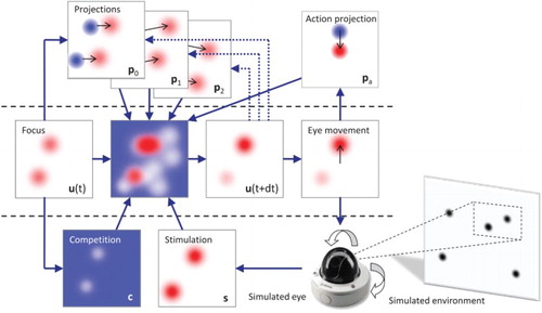
Figure 3. Architecture of the ANF model. The model first includes the lateral interaction ($\mathit{c}$) and integration of input stimulation ($\mathit{s}$) from the DNF model. It also integrates the projections (${\mathit{p}}_{\mathit{k}}$ with weight $w_k$) from the PNF model, themselves evaluated based on their ability to predict the current (here-and-now) location of the target (${\hat{\mathit{p}}}_{\mathit{k}}$). In addition, the model also controls eye movements (a), and thus can predict the associated transformations on the visual field to be facilitated by a projection of activity (${\mathit{p}}_{\mathit{a}}$) on the neural field. At each simulation time step, all components are combined with the neural field potential $\mathit{u}\left(t\right)$ to produce $\mathit{u}(t+\mathrm{d}t)$.

This attractor results from the combined effect of both ${\mathit{p}}_{\mathit{a}}$ and ${\mathit{p}}_{\mathit{k}}$ projections, as well as the stimulation, when they are symmetrical near the position ${\mathit{v}}_{\mathit{s}}\mathrm{d}t$ in the neural field reference frame. The peak may thus only be stabilised in the direction of the target motion and slightly away from the neural field centre. Despite the resulting small lag, this allows at the same time to continuously test the validity of different projections, while limiting the need to learn regularities in the entire visual field. An accurate alignment between the gaze and target directions would be possible by directly associating the eye movements with projections, and by simultaneously estimating the similarity between the performed and proposed movement, as well as drifts in the peak location (reflecting a mismatch between the expected and actual target motion). Such an approach based on sensorimotor contingencies in the context of active vision has been used in Quinton, Catenacci, Barca, and Pezzulo (2014) and Catenacci, Quinton, and Pezzulo (2014), but the subsequent increase of dimensionality of the learning space is better suited to well-structured stimuli. Here on the contrary, a small lag behind the target (at least momentarily) makes the decoupling of the target foveation and the oculomotor behaviour possible, since the validity of the associated projections can be estimated when the peak grows or shifts slightly away from the centre of the neural field. As a consequence, ${\mathit{p}}_{\mathit{k}}$ and ${\mathit{p}}_{\mathit{a}}$ can be acquired separately, and as the peak is expected to converge to a fixed location in the visual field, the problem of estimating the effect of ${\mathit{p}}_{\mathit{k}}$ on the peak movement in the PNF model dissolves.

To conclude this section, adopting an active vision approach by coupling eye movements with the neural field dynamics yields two main positive consequences: (1) learning the regularities becomes simpler, as only the central part of the visual field becomes critical for the accurate tracking of a target (a process which would in fact be facilitated by a non-homogeneous visual stimulation), (2) inertia in the equation still allows to filter out noise and distractors, but the constraint on target speed is reduced, as physical motor actions now replace peak movements (the system converges to a sensorimotor fixed point attractor, instead of a limit cycle in the visual space alone).

2.4. Simulation parameters and performance metrics

Before turning to the results, and to facilitate their reproducibility, we here specify the model parameters and exact simulation scenarios. As the ANF model is equivalent to the PNF model in the absence of eye movements and associated projections, and the PNF model to a DNF model by only considering projections with ${\mathit{v}}_{\mathit{k}}=\mathbf{0}$ (instead of setting $\alpha =0$ as previously described), we used the exact same parameter values for all simulations. The description, symbol and value (or range of values) for all parameters from the DNF, PNF and ANF equations are reported in Table 1. Although the number of parameters may seem elevated, they are not independent for a given objective behaviour (such as tracking a target). For instance, increasing the time constant τ facilitates noise filtering, but for the system to remain sufficiently reactive to track a rapidly moving target, the kernel usually needs to be simultaneously adjusted. For any given parameters, increasing the speed of the moving target, the number of distractors or the level of noise in the signals sooner or later breaks the expected performance of the system. Parameters have here initially been optimised using genetic algorithms for maximising the tracking performance of the DNF model (Quinton, 2010). This way, and by not retuning the parameters for the PNF and ANF models, we opt for the worst case conditions, where performance improvement due to the model extensions are minimised and can be hardly be explained by confounding factors.

As the objectives of this paper deal with detecting and tracking a moving target through different types of eye movements, we do not include distractors in the stimulation, and thus simply present a single noisy stimulus defined by: (14) $\mathit{s}(\mathit{x},t)=\hat{f}\left(A_s{\mathrm{e}}^{-\parallel {\mathit{x}}_{\mathit{s}}-\mathit{x}{\parallel }^2/{{\sigma }_s}^2}+ϵ\right)$(14) with ε being a white noise component sampled in $\mathcal{N}(0,{\sigma }_{ϵ})$, while $\hat{f}$ is a saturation function of unity slope (rectified linear unit), simply guaranteeing the stimulation values remain within $[0,1]$. ${\mathit{x}}_{\mathit{s}}$ is the centre of the Gaussian target profile, as used for instance in Equation (12b(12b) $\begin{array}{rl}{\mathit{x}}_{\mathit{s}}(t+dt)& ={\mathit{x}}_{\mathit{s}}\left(t\right)-{\mathit{x}}_{\mathit{a}}\left(\mathit{a}\right(\mathit{u}\left(t\right))={\mathit{x}}_{\mathit{s}}(t)-{\mathit{x}}_{\mathit{u}}(t)-\eta ,\end{array}$(12b) ), whose trajectory varies between results subsections. The dispersion of the stimulus distribution ${\sigma }_s$ could in theory be a free parameter, but should nevertheless be constrained by initial visual preprocessing steps for the tracking system to perform efficiently. As stated in Gepperth (2014), DNFs “contain a data model which is encoded in their lateral connections, and which describes typical properties of afferent inputs. This allows to infer the most likely interpretation of inputs, robustly expressed through the position of the attractor state”. Therefore, ${\sigma }_s$ is here taken equal to ${\sigma }_{+}$ to converge on near Bayesian optimal decisions.

To characterise the performance of the computational system, we rely on two complementary measures. First, an error signal estimates the distance $d_e$ between the centre of the field of view ${\mathit{x}}_{\mathit{f}}$ and the actual target location ${\mathit{x}}_{\mathit{s}}$. Since one cannot expect the system to focus on the target before it has been presented, the time variable is adjusted to guarantee that the target should be visible for any $t\in [0,T]$, with T corresponding either to the disappearance of the target, or the end of the simulation. Thus, we can estimate the mean error distance $\overline{d_e}$ as: (15) $\overline{d_e}=\frac{1}{T}{\int }_0^{\mathrm{T}}\parallel {\mathit{x}}_{\mathit{f}}-{\mathit{x}}_{\mathit{s}}\parallel \mathrm{d}t.$(15) Assuming that the target location varies during the entire simulation (either continuously when tracking a single moving target, or with discontinuities when switching between static targets), this error increases drastically when the target his lost (since ${\mathit{x}}_{\mathit{f}}$ will be no more matching ${\mathit{x}}_{\mathit{s}}$). Also, it is inflated when the peak lags behind the target (positive $\parallel {\mathit{x}}_{\mathit{f}}-{\mathit{x}}_{\mathit{s}}\parallel$ distance) or if the peak relaxes before focusing at a new position (with a maximal distance just before a new saccade is performed).

The characterisation of saccadic movements usually relies on a shift in signal frequency. In the case of experimental data on eye movements, they usually correspond to stereotyped profiles with speeds reaching up to ${800}^{\circ }$/s (in the monkeys) and lasting only a few milliseconds (<200 ms). Most eye-tracking hardware or analysis software rely on delay or speed thresholds to classify movements into saccades and fixations. Because of the temporal discretisation of the system used in the simulations, the movement speed is at best estimated over a single time step ($\mathrm{d}t$). The saccade, catch-up saccade and smooth pursuit movement distinction thus qualitatively depends on the instantaneous speed of the movement. Although small movements can be generated at each time step as long as the activity over the field remains high enough (over the action threshold), large amplitude movements (of high speed, and thus saccadic) cannot be sustained over several time steps. The same dynamical system thus generates: (1) continuous movements with an adaptive instantaneous speed defined as the derivative between successive locations, (2) saccadic movements, which induce a large change in field stimulation, and thus require the field to relax over several time steps (through lateral inhibition) before another movement can be generated (once the activity reaches again the action threshold).

To more accurately describe the performance of the system, we want to differentiate intervals during which smooth pursuit movements are made with a small lag, from series of small amplitude saccades. Following the previous paragraph, and from the dynamical system perspective adopted in this paper, the fundamental difference comes from the nonlinearity introduced by the action threshold, with smooth tracking simply corresponding to a maximal field potential maintained above $u_a$ over several time steps. Relying on the temporal discretisation of the equations, we thus define a saccade-like movement to occur whenever $a_{\mathrm{saccade}}=1$, following Equation (16(16) $a_{\mathrm{saccade}}\left(t\right)=\left\{\begin{array}{ll}1,& \mathrm{if}\parallel \mathit{u}\left(t\right){\parallel }_{max}\ge u_a\mathrm{and}\parallel \mathit{u}(t-dt){\parallel }_{max}<u_a,\\ 0,& \mathrm{otherwise}.\end{array}\right.$(16) ). (16) $a_{\mathrm{saccade}}\left(t\right)=\left\{\begin{array}{ll}1,& \mathrm{if}\parallel \mathit{u}\left(t\right){\parallel }_{max}\ge u_a\mathrm{and}\parallel \mathit{u}(t-dt){\parallel }_{max}<u_a,\\ 0,& \mathrm{otherwise}.\end{array}\right.$(16) For the purpose of differentiating smooth pursuit and saccadic eye movements when they hold the same error statistics $\overline{d_e}$, we introduce a second measure as the number of saccades performed during the entire simulation. Numerically, this is computed as the sum of $a_{\mathrm{saccade}}\left(t\right)$ for $t\in [0,T]$. The time period is set to be consistent with Equation (15(15) $\overline{d_e}=\frac{1}{T}{\int }_0^{\mathrm{T}}\parallel {\mathit{x}}_{\mathit{f}}-{\mathit{x}}_{\mathit{s}}\parallel \mathrm{d}t.$(15) ), but no saccade should be performed outside this time window when no target is presented. Combining the two measures is therefore necessary, as losing a target only increases $\overline{d_e}$, since no saccade is performed afterwards, thus lowering the relative number of saccades performed as time passes when compared to an accurate tracking behaviour. The prototypical combinations of the tracking statistics and their interpretation are synthesised in Table 2.

Table 2. Tracking statistics and their interpretation based on the type of target dynamics.

	Tracking error	Nb of saccades	Behaviour
Target dynamics	$\overline{d_e}$	$\sum _t{a}_{\mathrm{saccade}}\left(t\right)$	interpretation
(all)	High	High	Random saccades (depending on noise/parameters)
Saltatory movement	Low	Low	Stable fixation on target
–	Low	High	Micro-saccades around target
–	High	Low	Continuous drift away from target
Smooth movement	Low	Low	A few catch-up saccades followed by smooth pursuit
–	Low	High	Catch-up saccades during the entire simulation
–	Medium	Medium	Alternation of fixations and saccades
–	High	Low	Target lost during the simulation

3. Results

The ANF model will be tested on different scenarios, to demonstrate its performance, analyse its fine-grained dynamics, and facilitate an incremental understanding of its behaviour. The following section thus covers targets with fixed positions over an extended period of time (thus reflecting how the visual system focuses on different features by alternating saccades and fixations), and targets moving along a continuous trajectory (thus testing the generation of catch-up saccades and smooth pursuit).

3.1. Fixational eye-movements

To evaluate the performance of the ANF model, we start by exploring the fine-grained characteristics of the simulated oculomotor dynamics on series of fixations. Using Equation (14(14) $\mathit{s}(\mathit{x},t)=\hat{f}\left(A_s{\mathrm{e}}^{-\parallel {\mathit{x}}_{\mathit{s}}-\mathit{x}{\parallel }^2/{{\sigma }_s}^2}+ϵ\right)$(14) ) to generate the sensory stimulation, ${\mathit{x}}_{\mathit{s}}$ is now sampled in the uniform distribution $\mathcal{U}(-.5+{\sigma }_s,.5-{\sigma }_s)$, thus guaranteeing that a well-defined peak of activity grows within the limits of the neural field, in response to a target present in the visual field. This avoids the need for a log-polar representation of the visual field (favouring the emergence of central peaks) or the use of a toric manifold (which is often adopted in computational studies to escape the boundary problems from the differential equation, for example, discussed in Rougier & Vitay, 2006). The location of the input stimulus remains the same for periods of 1 second, before jumping to a new random position (sampled from the same distribution). Although an adaptation mechanism responsible for perceptual fading, an inhibition of return mechanism, or top-down modulations of activity should be implemented to reflect realistic dynamics of saccades and fixations, as well as to replicate the usual frequency of saccades (e.g. during free viewing or cognitive tasks), this is not the focus in the current paper and has been explored elsewhere (Quinton et al., 2014). The current system dynamics nevertheless parallels computational models of visual attention based on saliency maps (Itti & Koch, 2001), where the target selection is based on lateral inhibition in recurrent neural networks in the original models (Itti, Koch, & Niebur, 1998).

The resulting sequence of fixations generated by the ANF model can be observed in Figure 4(a), which is a projection of the visual field centre along the horizontal axis (i.e. first component of the ${\mathit{x}}_{\mathit{f}}$ vector) as a function of time. The complete trajectory of the target may cover a large part of the environment, captured by a succession of saccades whose amplitude yet never exceeds half the size of the visual field (due to the constraints introduced in the previous paragraph). The uniform distribution used to sample the target location leads to a random-walk behaviour, with 10 fixations visible in Figure 4(a).

Figure 4. Representative trajectory of the Cartesian visual field coordinates in the environment, when focusing on targets adopting a new random position every second. The left figure reflects the relative complexity of the trajectory, with a sequence of saccades and fixations matching the stimulus dynamics, but also random fluctuations and micro-saccades. The right figure displays the power spectrum of the movements along the x-axis, with a decreasing. (a) Simulated eye position along the x-axis and (b) Power spectrum of the movements along the x-axis.

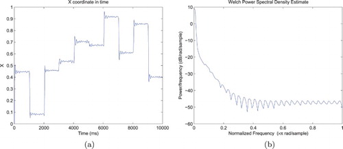
The oscillations visible in Figure 4(b) are in part due to the temporal discretisation of the differential equation combined with the choice of bandwidth resolution for the Welch power spectral density estimate, but also reflect the closed-loop interactions between the projections and neural field for a fixed target location. Nevertheless, and despite the stochasticity of the simulation, a decreasing power as frequency increases is systematically found. As stated by Astefanoaei, Creanga, Pretegiani, Optican, and Rufa (2014), “using a log-linear scale the visualisation of the power spectrum of either random or chaotic data may be a broad spectrum but only chaotic signals are expected to emphasise a coherent decrease of the square amplitude with the frequency increase”. Following the methodology they used when studying how human execute saccadic and fixational eye movements in response to red spots visual stimuli, we qualitatively replicate human behaviour (Figures 2 and 4 of their paper, respectively, corresponding to the trajectory and power spectrum on the horizontal axis, that is, Figure 4(a, b) here). Studying the movements separately for each fixation, the power spectral density demonstrates the same decreasing trend. Also, adopting the same statistics to characterise the temporal dependency in the eye trajectory, we found high values for the Hurst exponent (M=.70, $\mathrm{SD}=.03$). Combined, these results demonstrate that the micro-movements performed by the system during fixations are neither purely oscillatory (where peaks should be observed on the power spectrum) nor purely fully driven by the stimulation noise (since we should find $H\approx .5$ for Brownian motion).

Although such descriptive statistics based on frequency distributions do not account for all characteristics of fixational eye movements, they are compatible with the frequency shift approach generally used to characterise the different types of eye movements (as introduced in previous section). Without a more refined model of eye movements, we cannot expect the current system to correctly approximate more than the frequency distribution of fixational eye movements (e.g. their spatial distribution). Indeed, motion is only induced by eye movements in this evaluation scenario, and projections are thus defined by Equation (13(13) $p_a(\mathit{x},t)=u(\mathit{x}-{\mathit{x}}_{\mathit{a}}(\mathit{a}\left(\mathit{u}\right(t-\mathrm{d}t\left)\right)),t-\mathrm{d}t)-u(\mathit{x},t-\mathrm{d}t).$(13) ). In absence of other projections that may distort space locally, and in presence of white noise in the external stimulation, the projected activity is also statistically anisotropic (the robustness of neural fields to such perturbations being one of their strength). Variability in the stimulation thus influences the estimation of target location, but do not introduce the asymmetries that are found in real visual environments and that would be amplified by the activation of context dependent projections (see next sections). As a consequence, and for static targets, the same pattern is observed for each fixation, and would be for any arbitrary projection direction (x-axis in Figure  4). With this model in mind, we can argue that fixations are the result of a balanced activity between opposing commands and associated projections. The equilibrium might not be perfect at all time, thus leading to fluctuations around the target location, but the dynamics of the system implies that the target will define a fixed point attractor. Thus, visual fixation can be conceived as a dynamic equilibrium in the visuo-oculomotor system, as proposed by neurophysiological studies (Goffart et al., 2012; Krauzlis et al., 2017).

In addition to the frequency distribution, we can also look at the movements generated by the system once the initial oscillations driven by the nonlinear dynamics have settled, that is, when the fixation conceived as an ideally fixed attractor has been reached. Such movements mainly appear a few hundred milliseconds after a peak has grown in the new central position, since the strong lateral inhibition of the current model prevents several peaks to be maintained near the action threshold ($u_a$). This naturally replicates the delay observed in humans from fixation offset to micro-saccades production, rather independently of the task performed (Otero-Millan et al., 2008). Even though micro-movements performed by the system during fixations (i.e. when the theoretical target location is stable) are partly driven by the sensory noise, the system responds through a coherent behaviour, with fluctuations in projection weights influencing the neural dynamics and generated eye movements. Although these movements are only the by-product of a target centring oculomotor behaviour yielded by fluctuating signals, they also contribute to locate the target within the visual field, increasing potentially the robustness of the gaze-related signals which guide the movements of, for example, the hand. More careful testing would be required to conclude on this part, but they may also contribute to increase the acuity of the system (see Ko, Poletti, and Rucci (2010) for related human experiments; Franceschini, Chagneux, Kirschfeldand, and Mücke (1991) for early experiments in the fly; Viollet (2014) for a review of visual sensors hyperacuity based on micro-eye movements). They may also contribute to cognitive demands at end (Hicheur et al., 2013) through the activation of task-dependent projections. Generalising to other movements and equilibria, a connection can be made with the slight and chaotic movements performed by the human body for keeping balance (Milton, Insperger, & Stepan, 2015).

3.2. Attractor dynamics on a moving target

In this section, we turn to stimuli crossing the visual field with a constant velocity. For the system to detect and track the moving target, we generated targets which followed rectilinear trajectories defined by: (17) ${\hat{\mathit{x}}}_{\mathit{s}}={\mathit{x}}_{\mathit{f}}+{\mathit{x}}_{\mathit{s}}={\mathit{v}}_{\mathit{s}}t,$(17) where ${\hat{\mathit{x}}}_{\mathit{s}}$ is the target location in the world coordinate system, which differs from the target position within the visual field coordinate system as it depends on ${\mathit{x}}_{\mathit{f}}$. Starting the simulation at a negative time $t\ll -0.5/{\mathit{v}}_{\mathit{s}}$ (but for ${\mathit{v}}_{\mathit{s}}=\mathbf{0})$ and setting the initial visual field position at ${\mathit{x}}_{\mathit{f}}=0$, the position of the target at t=0 should be ${\mathit{x}}_{\mathit{s}}=0$ (i.e. the centre of the visual field). This equation thus guarantees the trajectory crosses over the visual field and passes through its centre, as long as no eye movements away from the initial position are produced by the system before the target enters the visual field. Although more complex trajectories could be used, they would be of no consequence for the explanatory power of the model. Also, this section additionally serves the purpose of introducing the results from the following section, in which we replicate empirical observations made in monkeys tracking a target adopting similar trajectories.

In this section, the system includes an additional projection corresponding to a constant velocity (${\mathit{v}}_{\mathit{k}}$ in previous sections), thus related to Equation (10(10) ${\mathit{p}}_{\mathit{k}}(\mathit{x},t)=u(\mathit{x}-{\mathit{v}}_{\mathit{k}}\mathrm{d}t,t-\mathrm{d}t)-u(\mathit{x},t-\mathrm{d}t).$(10) ). As previously, we also consider a correct map has been learned for the eye movements (associated with ${\mathit{p}}_{\mathit{a}}$ from Equation (13(13) $p_a(\mathit{x},t)=u(\mathit{x}-{\mathit{x}}_{\mathit{a}}(\mathit{a}\left(\mathit{u}\right(t-\mathrm{d}t\left)\right)),t-\mathrm{d}t)-u(\mathit{x},t-\mathrm{d}t).$(13) )) to centre any target located anywhere in the visual field. Figure 5 illustrates a few representative dynamics by plotting the distance between the visual field centre and the actual target location (metrics $d_e$) as a function of simulation time, running 5  s simulations. They represent particular instances in the target speed continuum ($\parallel {\mathit{v}}_{\mathit{s}}\parallel \in [0,+\mathrm{\infty })$) with a projection corresponding to a static target (${\mathit{v}}_{\mathit{k}}=\mathbf{0}$). This configuration allows evaluating the behaviour of the original DNF model endowed with the generation of eye movements. With the specific delay parameter chosen, we indeed obtain ${\mathit{p}}_{\mathit{k}}=\mathit{u}(t-\mathrm{d}t)$, so that the dynamics of the original equation is maintained, yet slightly altered depending on the value of α in Equation (7(7) $\hat{\mathit{s}}\left(t\right)=\alpha \mathit{p}\left(t\right)+(1-\alpha )\mathit{s}\left(t\right),$(7) ). The dynamics on the figure can be classified as follows:

• For a static stimulus (${\mathit{v}}_{\mathit{s}}=\mathbf{0}$), a peak grows at the centre of the field after 200ms (since ${\mathit{x}}_{\mathit{s}}\left(t\right)=\mathbf{0}$, $\mathrm{\forall }t$), followed by small and slow movements in part driven by stimulation noise (leading to a very small yet non-zero distance).

• For stimulus speed values in $[.5,1]$, the target is detected before it reaches the field centre, generating an interceptive saccade to it (drop in error distance around t=−750ms for $\parallel {\mathit{v}}_{\mathit{s}}\parallel =.5$, and −400 ms for $\parallel {\mathit{v}}_{\mathit{s}}\parallel =1$).

• For stimulus speed values in $[1.5,2]$, the target passes through the field and is captured before exiting at $t\approx 200$ ms, the initial saccade being followed by an alternation of drifts and catch-up saccades, before the target is lost at $t\approx 3300$ ms for $\parallel {\mathit{v}}_{\mathit{s}}\parallel =1.5$ and $t\approx 1900$ ms for $\parallel {\mathit{v}}_{\mathit{s}}\parallel =2$.

• For extreme speed values ($\parallel {\mathit{v}}_{\mathit{s}}\parallel \ge 2.5$), the target just crosses the field in less than 500 ms, so that no peak emerges and the target has not been detected in any of the simulations.

Figure 5. Distance between the visual field centre and actual target coordinates ($d_e$) as a function of time, for a system with a null projected velocity (${\mathit{v}}_{\mathit{k}}=\mathbf{0}$) and targets moving along a rectilinear trajectory at various speeds ($\parallel {\mathit{v}}_{\mathit{s}}\parallel \in \{0,.5,1,1.5,2,2.5\}$). This allows testing the behaviour of the original DNF model endowed with the ability to generate of eye movements. All stimuli are designed to reach the centre of the visual field at t=0 in absence of eye movements. Dotted lines correspond to the extrapolated target trajectories in the field reference frame, where no eye movement would be performed. For small increasing speeds, the target is detected and tracked with an increasing lag. For larger amplitudes, the target is captured and tracked through sequences of catch-up saccades. For extreme increasing speeds, the target gets lost sooner, or not even detected (for $\parallel {\mathit{v}}_{\mathit{k}}\parallel =2.5$). Values increasing beyond .5 betray a loss of target (i.e. target exiting the visual field that cannot be captured again).

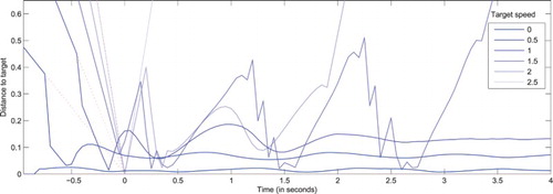
Figure 6 illustrates complementary dynamics, when stimulus speed is fixed at $\parallel {\mathit{v}}_{\mathit{s}}\parallel =2$ and the projection speed increases, again for a system with a single projection for expected (observed) movements. For a projection corresponding to a target expected to be static (${\mathit{v}}_{\mathit{k}}=\mathbf{0}$), the behaviour observed in Figure 5 for $\parallel {\mathit{v}}_{\mathit{s}}\parallel =2$ is roughly reproduced. Yet, the fact that the target is now tracked during the entire simulation (instead of being lost at $t\approx 3300$ ms) reflects the chaotic nature of the system. The precise time of interception and the number of catch-up saccades also vary. Thus, the boundaries between the categories drawn previously must be considered as fuzzy and dependent upon the exact stimulation dynamics.

Figure 6. Distance between the visual field centre and actual target coordinates ($d_e$) as a function of time, for a system presented with targets moving along a rectilinear trajectory with a constant speed ($\parallel {\mathit{v}}_{\mathit{s}}\parallel =2$), but with different projected velocities, all matching the motion direction of the target, but with different amplitudes ($\parallel {\mathit{v}}_{\mathit{k}}\parallel \in \{0,.5,1.5,2.5\}$). All stimuli are designed to reach the centre of the visual field at t=0 in absence of eye movements. As the projected speed gets closer to its optimal value, fewer catch-up saccades are performed, and the target is tracked with a diminishing lag. As discussed in the main text and in order to correctly estimate the validity of projections, the lag is never fully cancelled.

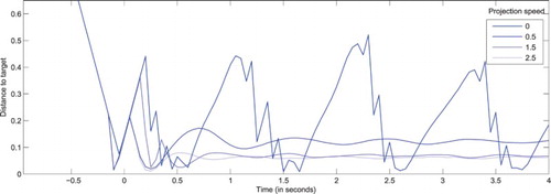
For projection speed values in $[.5,2.5]$, the target is intercepted earlier, centred through a smaller number of catch-up saccades, and then tracked with a decreasing lag when the projection speed gets closer to the actual target speed. The direct comparison of the projection and target speed is made possible by the simple coordinate transformations involved here, yet optimal tracking never occurs for perfectly matching speeds. Small oscillations still appear, reflecting that the relaxation of a slightly lagging peak facilitates its movement, then leading to its maximal activity building up again (see Quinton & Girau, 2011, for additional details in the context of the PNF model). The system thus performs the expected behaviour of classical DNFs when presented with static targets, by converging to a stable attractor in the visual space, yet performing eye movements to correctly compensate the target elevated speed.

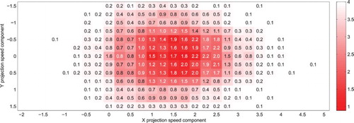
To get a broader view of the dynamics, and to be able to obtain statistically meaningful results, repeated simulations have been performed to average out the stochastic components of the equations. We can then characterise the conditions under which the system is able to detect and track the target, using both the error distance ($d_e$) and number of saccades ($\sum a_{\mathrm{saccade}}$), varying both ${\mathit{v}}_{\mathit{s}}$ and ${\mathit{v}}_{\mathit{k}}$. 200 runs of 5  s have been executed for each combination of ${\mathit{v}}_{\mathit{s}}$ and ${\mathit{v}}_{\mathit{k}}$ (fixed throughout each simulation). Figure 7 represents the performance of the system when the stimulus adopts a horizontal velocity set at ${\mathit{v}}_{\mathit{s}}=(2,0)$, and the projection speed ${\mathit{v}}_{\mathit{k}}$ varies in $[-2,2]\times [-1.5,1.5]$. The gradient (both in colour for error distance and figures for the number of saccades) reflects the optimality of performance for projection speed close to the target actual speed and the very progressive loss of performance when parameters deviate. Yet, in accordance with earlier PNF results and due to the neural dynamics, the optimal configuration does not correspond to ${\mathit{v}}_{\mathit{k}}=(2,0)$ but to ${\mathit{v}}_{\mathit{k}}\approx (1.5,0)$, with less than two (interceptive and catch-up) saccades to definitely capture (foveate) the target. Indeed, the dispersion in both metrics is very low for near optimal configurations. The number of saccades here never reaches high values due to the excessive speed of the target, rapidly lost without the proper projection (please refer to Table 2 as a guide for the combined colour and figure interpretation). The variability and decimals in the average number of saccades performed reflect the stochastic nature of the process. Values of 0.1 may for instance correspond to targets which have been intercepted in 5% of the simulations (10/200), but where immediately lost.

Figure 7. Mean distance between the simulated eye and real target coordinates after t=0 (colour gradient) and average number of saccades per trial (figures), for a target moving at $\parallel {\mathit{v}}_{\mathit{s}}\parallel =2$ units/second along the horizontal axis ($1\mathrm{unit}=\mathrm{visual}\mathrm{field}\mathrm{width}$). Each cell corresponds to 200 simulations of the system running with a single projection, with the corresponding projection velocity components indicated along the axes. A bell-shaped profile appears around the target speed coordinates (with low error, and less than 2 catch-up saccades to capture the target), reflecting the discrimination capabilities of the projections.

To test the performance of the system on slow targets (i.e. checking that the performance does not degrade under weaker constraints), and to test the limits of the system with targets adopting extreme speed values, the synthesis of complementary simulations is shown in Figure 8. While both target and projection velocity this time adopt the same direction, their amplitude both vary, with $\parallel {\mathit{v}}_{\mathit{s}}\parallel \in [0,3]$ and $\parallel {\mathit{v}}_{\mathit{k}}\parallel \in [-2,5]$. The behaviour can again be classified as follows:

• $\parallel {\mathit{v}}_{\mathit{s}}\parallel =0$ (first row with static stimulus): Even with extreme projection speeds, convergence on target occurs within one or two saccades, and the tracking error remains low. This demonstrates that the internal projection does not overcome the input stimulus.

• $\parallel {\mathit{v}}_{\mathit{s}}\parallel \in (0,1.25]$ (low target speed): The projection hinders the correct tracking of the target if the projection velocity is opposed to the target motion. Even though the system is still able to track the target with a relatively low error, the number of catch-up saccades increases drastically when the target speed increases (up to 2.5 saccades/second), highlighting the need for correct projections when they become necessary for capturing the target.

• $\parallel {\mathit{v}}_{\mathit{s}}\parallel \in (1.25,2]$ (high target speed): The target is most often lost with incorrect projections, while performance improves with smaller lag and fewer catch-up saccades for target and projection speeds which are compatible. Symmetrically, the target is lost for excessive projection speeds. The results for $\parallel {\mathit{v}}_{\mathit{s}}\parallel =2$ statistically match those from Figure 7 for horizontal projection velocities (row with vertical component equal to 0). The nonlinearity of the system can be observed on the figure, as there the relation between the target speed and equivalent optimal projection on the neural field is clearly nonlinear: $\parallel {\mathit{v}}_{\mathit{k}}\parallel \approx 3$ for $\parallel {\mathit{v}}_{\mathit{s}}\parallel =1.5$, thus facilitating the relaxation of a too stable peak, while $\parallel {\mathit{v}}_{\mathit{k}}\parallel \approx 1.5$ for $\parallel {\mathit{v}}_{\mathit{s}}\parallel =1.75$, thus reinforcing a peak that already tends to disappear.

• $\parallel {\mathit{v}}_{\mathit{s}}\parallel \in (2,+\mathrm{\infty })$ (extreme stimulus speed): The target is not efficiently tracked in any of the simulations. At best, a few interceptive or catch-up saccades are performed before the target is lost (leading to average numbers of saccades below 1, and very high tracking error).

Figure 8. Mean distance between the simulated eye and real target coordinates after t=0 (colour gradient) and average number of saccades per trial (figures), for a target moving at different speeds and for various projection speeds (both velocity vectors remaining collinear). Each cell corresponds to 200 simulations of the system running with a single projection, with the target and projection speed values indicated along the axes.

In all of these simulations, and for the selected tracking statistics, we find that the ANF model outperforms the original DNF model endowed with the generation of eye movements (see configuration ${\mathit{v}}_{\mathit{k}}=(0,0)$ in Figure 7 and $\parallel {\mathit{v}}_{\mathit{k}}\parallel =0$ in Figure  8). Integrating all previous results, the dynamics of the system as a function of the stimulation and projections can be simplified as a graph represented in Figure 9, where nodes correspond to specific dynamics or attractors of the system, and transitions to changes (or maintenance) in projection or target speed. The transitions can be described as follows:

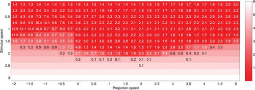
1. No spatiotemporally coherent stimulation is provided to the system, and the field potential $\mathit{u}$ remains close to its resting level (fluctuations being due to sensory noise).

2. A target crosses the visual field, but is yet to be detected and intercepted by the system.

3. The target is detected (relatively) early due to its low to medium speed, or thanks to the facilitatory effect of a compatible projection. Nevertheless, the peak always builds with a small lag relatively to the actual target position.

4. As soon as a peak builds above the threshold for eye movement generation ($u_a$) and away from the centre of the visual field, the movement brings the target to a closer location from the centre. As the target continues in the same direction, the peak is either continuously reinforced or rapidly reaches the threshold again if it is slightly relaxed, hence generating another catch-up saccade.

5. If the peak progressively approaches the position where the projection matches the target here-and-now location, the peak is maintained at a maximal level of activity, and a stable fixed point attractor is reached.

6. As the peak activity is maintained above the eye movement threshold, continuous smooth pursuit movements are generated.

7. If the target crosses the field at a higher speed (vs. (C) above), the peak will only build later, just before the target leaves the visual field.

8. An interceptive saccade of greater amplitude is generated. The peak will then immediately decay below the threshold, since the target now stimulates the centre of the field while the decaying peak of course remains in its previous location.

9. The relaxation of the peak (or at least its diminishing amplitude) allows a new peak to emerge, when the target is again about to leave the visual field. This alternation generates a sequence of saccades and fixations, which can simply be viewed as an amplified dynamics compared to transition (D).

10. If the target crosses the field at an extreme speed (at least relatively to the equation time constant and to (C) and (G) above), no peak is fully formed, and the field activity does not reach the eye movement threshold before the target leaves the visual field. Similar transitions occur from several other states if the stimulus speed increases or if random fluctuations are sufficient to destabilise the peak or delay its formation. With a more general projection model, this should happen when the target adopts an unexpected movement at a sufficiently high speed.

11. Once the target is lost and any activity relaxes on the neural field, the system returns to its initial idle state, since no active exploration of the environment is implemented here.

Figure 9. Illustration of the ANF model dynamics in presence of a moving target following a rectilinear trajectory with constant speed. Adopted states and transitions depend on the target dynamics and internal projection of activity, and are thus implicitly represented here using arrows: low or compatible speeds with single-headed arrows, high speeds and/or medium discrepancy with double-headed arrows, extreme speeds or high discrepancy with triple-headed arrow. Apparent target position in the visual field is represented as a dashed circle while the neural field peak is represented by a Gaussian profile activity whose intensity reflects the peak amplitude. Please refer to the main text for the detailed description of the labelled transitions.

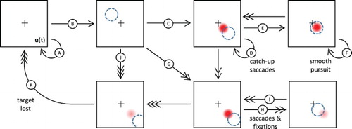
3.3. Learning with catch-up saccades and smooth pursuit

In all previously described results, we have assumed the projection was fixed so that trials were totally independent. Here, we aim at replicating observations made by Bourrelly, Quinet, and Goffart (2013) and Bourrelly, Quinet, Cavanagh, and Goffart (2016), demonstrating in macaque monkeys that the ability to accurately pursue a moving target is not spontaneous but must be learned. Over the course of several trials and training sessions, the monkeys improve their ability to foveate the moving target with slow eye movements of progressively increasing velocity while at the same time, the number of catch-up saccades is reduced, as if the foveation system attempted to synchronise the movement of the eyes with the current here-and-now location of the target. We also want to test whether the model fits other empirical results obtained by Quinet and Goffart (2015), showing how the monkey brain differently extrapolates transient target motions depending upon the rate of change in speed.

As a consequence, we try here to qualitatively reproduce in silico the paradigm used in these experiments. A fixed target is initially presented at ${\mathit{x}}_{\mathit{s}}=(0,-0.3)$ from t=−1 s. This artificial fixation point is removed before t=0 (leaving 200 ms for the peak to relax), and replaced by a target moving horizontally with a constant velocity ${\mathit{v}}_{\mathit{s}}=(1.4,0)$, starting from ${\mathit{x}}_{\mathit{s}}=(0,0)$. The speed amplitude of 1.4 is chosen in order to make it possible for the system to track the target in the absence of correct projection, even though this may often require several catch-up saccades, as the system demonstrates a large variability in performance for this configuration (see Figure 8). At t=0.8 s, the target disappears, allowing to test the continued dynamics of the system without stimulation. For every trial, the exact same stimulation dynamics is reproduced, except for the sensory noise. During each trial, the eccentricity of the peak is estimated, reflecting the lag of the system and providing a 2D gradient towards the optimal projection (and thus predicted velocity). We thus again assume all mappings between the neural field activity and eye movements and projections have been learned, reducing the dimensionality of the problem without much changing its complexity and characteristics. Nevertheless, convergence relies on the convexity of the 2D problem, which is illustrated in Figure 7 with the tracking error following a bell-shaped profile based on the 2D projection velocity. The projection (associated to the projection velocity) is arbitrarily updated at the end of each trial, in order to make the connection with previous sections simpler, and to guarantee a correct estimation of the gradient over a sufficient period of time. Since we have previously noted that the peak should grow at an eccentric location reflecting the projection speed, we can directly update the estimate iteratively as follows: (18) ${\mathit{v}}_{\mathit{k}}=(1-\beta )\times {\mathit{v}}_{\mathit{k}}+\beta \times \frac{{\overline{\mathit{x}}}_{\mathit{u}}}{\mathrm{d}t},$(18) which is a time discretised version of a differential equation with relaxation and input from the current trial estimate. β is set to $.05$ in the following simulation, which corresponds to a 40 s integration time constant for trials of 2 s. The estimate of the average peak eccentricity ${\overline{\mathit{x}}}_{\mathit{u}}$ is computed for $t\in [0.8,T]$, in order to let enough time for the peak to emerge, and eliminate the influence of the static target presented at the beginning of each trial. Of course, a more complete version of the model should learn to predict the dynamics of the entire trial (e.g. exact timing at which the moving target appears), but this would no more correspond to the simple case of linear movements studied here.

Figure 10(a) displays the evolution of ${\mathit{v}}_{\mathit{k}}$ components over the course of 1000 trials. Although convergence occurs rapidly, the continuing variations are due to the signal/noise ratio in the model and the chaotic nature of the performance, limiting the precision of the estimate with the current integration scheme from Equation (18(18) ${\mathit{v}}_{\mathit{k}}=(1-\beta )\times {\mathit{v}}_{\mathit{k}}+\beta \times \frac{{\overline{\mathit{x}}}_{\mathit{u}}}{\mathrm{d}t},$(18) ). Figure 10(b) illustrates the dynamics of the ANF system on two representative trials, at the beginning of the simulated experiment (trial #10) and at the end (trial #1000). Table 3 also reproduces the two statistics used throughout this paper for the previously mentioned trials, as well as the peak eccentricity (translating the lag of the system in spatial terms). At the end of the learning period, the mean tracking error is highly reduced much below the peak dispersion ${\sigma }_{+}$, which equals to $.1$ in this paper. The eccentricity of the peak for trial #1000 is reaching the exact value for which $\parallel {\mathit{v}}_{\mathit{s}}\parallel =\parallel {\overline{\mathit{x}}}_{\mathit{u}}\parallel /dt$ ($1.4=0.07/0.05$), but does not match the system projection speed for the same trial (${\mathit{v}}_{\mathit{k}}=(1.23,0.09)$). Also, the number of saccades drops to 2, with an interceptive saccade followed by a single catch-up saccade. The eye movement is almost perfectly synchronised with the target motion. This remains true for a few milliseconds after the target disappears and until the relaxation of the peak at $t\approx 950$ ms, demonstrating the robustness and inertia of the PNF equation, here transferred into the sensorimotor system of the ANF model. A decrease in eye movement speed is observed in the empirical data once the target has disappeared, but is not present in the current simulations. This is simply because a single projection is considered in this part of the simulations; without competition between projections corresponding to different hypotheses, and in absence of a spatiotemporally coherent stimulus, the peak dynamics is only driven by the single active projection, at least until the peak relaxes below the action threshold. We thus qualitatively replicate the dynamics and evolution of visual tracking reported by Bourrelly et al. (2013, 2016) and Bourrelly, Quinet, and Goffart (2014), while the system also statistically lags behind the target, thus also demonstrating that no prediction of the future location of the target is needed for the system to track the target at its current (here and now) location. For individual trials (like #10), there might be a few exceptions, but these are due to noise, incorrect target location estimates, or excessive overestimation of the target speed at the early stages of the learning process.

Figure 10. Illustration of the learning dynamics of the ANF system when updating the projection of activity on the neural field after each trials, reproducing experimental data from Bourrelly et al. (2016). (a) The projection speed components (X and Y) rapidly converge to relatively stable values (dashed lines for the asymptotic means), yet different from the target speed components (plain lines at 1.4 for X, and 0 for Y), due to the complex neural field dynamics. (b) Representative trajectories for trials #10 and #1000. The behaviour drastically changes, with an earlier capture of the target, a reduction in the number of catch-up saccades, the dominance of smooth pursuit, and the continuing tracking at the here-and-now position of the target even after its disappearance (dashed line corresponding to the target trajectory, and stopping at t=.8 s). (a) Convergence of the “projection speed” and (b) Trajectory samples before/after learning.

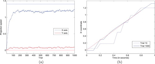
Table 3. Performance statistics for representative trials during learning.

Run	#10	#1000
Mean peak eccentricity ($\overline{\parallel x_u\parallel }$)	0.193	0.070
Mean tracking error ($\overline{d_e}$)	0.085	0.027
Number of saccades ($\sum a_{\mathrm{saccade}}$)	5	2

4. Conclusion and discussion

Using the formalism of DNF theory, this paper brings a proof-of-concept model which is able to replicate different types of eye movements (rapid saccade or slow pursuit) that primates make in response to a visual target, static or moving. More importantly, the qualitatively distinct eye movements emerge as attractors in a sensorimotor dynamical system, without altering the neural field parameters. Once the usual parameters are set, transitions between the two types of eye movements occur depending on the target eccentricity and speed, the amount of noise, as well as the a priori knowledge about the possible target trajectories. Slightly altering the neural dynamics through delayed projections of activity is indeed often sufficient to switch from one eye movement type to the other, and to outperform the original DNF model endowed with the same mechanism for eye movement generation. For instance, anticipating the target motion may transform a limit cycle attractor (corresponding to series of saccades with an oscillating peak on the neural field) into a fixed-point attractor in the sensorimotor system (corresponding to a smooth pursuit tracking behaviour), by reducing the peak lag and eccentricity of the target in the visual field. Put differently, our results underline the role of both embodiment and timing, since the very same sensorimotor dynamical system leads to apparently distinct visuomotor behaviours, depending on the precise interactions between the dynamics of the neural field, eye movements and target motion.

Although variations of the neural field parameters have not been tested in this paper, most configurations allowing attentional properties to emerge in classically DNF models can be exploited in the PNF and ANF contexts. Also, even though variations in the parameters would alter the results, we also indirectly tested the additional flexibility provided by the addition of projections and eye movements. By learning the optimal projection the system should use to perfectly synchronise with rapidly moving targets, we demonstrated how the system may compensate for an initial lack of performance and for possible inter-individual differences in neural dynamics.

Relatively to the task at hand, parameters are usually adjusted by considering the trade-off between the adaptability and stability of the system (e.g. by preventing or facilitating the relaxation of the peak of activity). This imposes limitations on the level of dynamics the system can cope with (e.g. target maximal speed), thus favouring the modelling of behaviours which can be characterised by a convergence on fixed attractors followed by instabilities, for instance with saccadic eye movements, by relying on temporary inhibition of the neural field activity to switch from one attended location to another. Of course, the intrinsic limitations of neurally plausible field dynamics remain, for example, by not artificially reducing the time constant in the original equation while increasing the temporal resolution of the simulation. Yet, these limitations are here transcended by the continuous coupling and mutual influence with the motor components. Instead of relying on phase transitions between stables states driven by predictions, observed or induced changes in the sensory flow, we turn to a unique sensorimotor dynamical system in which stable states are not exclusive of movement.

In the near future, the generalisation of the results to more complex motions should be tested, relying on the transition and interpolation between expected local trajectories. Target trajectories with a wide range of shapes and dynamics can be computationally studied, for instance aiming at replicating the empirical results on accelerating or decelerating targets (Bourrelly, Quinet, & Goffart, 2015). Further developments are yet required to better model and explain some key principles of the oculomotor dynamics. As briefly discussed in previous sections, the integration of an adaptation mechanism responsible for perceptual fading would allow reflecting realistic dynamics of saccades and fixations. Also, the hypotheses about the functional role of fixational eye-movements (here induced by noise or projections) could be explored by activating or deactivating various components of the model. On a related note, this line or work could extend and bridge the gap with systems which also rely on dynamical systems and dynamical neural fields to model perceptual decision-making and fixation patterns on structured visual stimuli (Quinton et al., 2014), as well as to detect and track objects of interest in presence of combined target-motion and ego-motion (Maggiani et al., 2016).

Finally, a preference for orienting gaze shifts that bring the target near the centre of the visual field was here assumed. Explanatory reasons for favouring such saccades can be computationally evaluated, for instance by adopting a retinotopic yet non-homogeneous representation of the visual field (with a greater accuity in the fovea, at the centre of the retina), as developed in Taouali et al. (2015). In addition to limiting the extent of the sensorimotor regularities to be learned, a saccade then also leads to the magnification of the target image. This over-representation of the target in terms of neurons can also be reversely seen as a local distortion of space-time, slowing down the apparent motion of the target relatively to the neural dynamics. Such mechanism and those developed in this paper are complementary, both facilitating the tracking of the target for given neural field parameters. These mechanisms should be integrated and their relative contributions evaluated in the future.

Disclosure statement

No potential conflict of interest was reported by the authors.

ORCID

J. C. Quinton http://orcid.org/0000-0001-8118-1752

L. Goffart http://orcid.org/0000-0001-8767-1867

Additional information

Funding

The research leading to these results has received funding from the French program “investissement d'avenir” managed by the Agence Nationale de la Recherche (ANR), from the European Union (Auvergne European Regional Development Funds) and from the “Région Auvergne” in the framework of the IMobS3 LabEx (ANR-10-LABX-16-01), as well as from the LabEx PERSYVAL-Lab (ANR-11-LABX-0025-01).

References

- Amari, S.-I. (1977). Dynamics of pattern formation in lateral-inhibition type neural fields. Biological Cybernetics, 27(2), 77–87. doi: 10.1007/BF00337259
- Astefanoaei, C., Creanga, D., Pretegiani, E., Optican, L., & Rufa, A. (2014). Dynamical complexity analysis of saccadic eye movements in two different psychological conditions. Romanian Reports in Physics, 66(4), 1038.
- Bar, M. (2007). The proactive brain: Using analogies and associations to generate predictions. Trends in Cognitive Sciences, 11(7), 280–289. doi: 10.1016/j.tics.2007.05.005
- Barandiaran, X. E. (2016). Autonomy and enactivism: Towards a theory of sensorimotor autonomous agency. Topoi, 1–22.
- Bell, C., Storck, T., & Sandamirskaya, Y. (2014). Learning to look: A dynamic neural fields architecture for gaze shift generation. In S. Wermter, C. Weber, W. Duch, T. Honkela, P. Koprinkova-Hristova, S. Magg, … A. E. P. Villa (Eds.), Artificial neural networks and machine earning – ICANN 2014, Lecture Notes in Computer Science (Vol. 8681, pp. 699–706). Cham: Springer.
- Bickhard, M. H. (1999). Interaction and representation. Theory & Psychology, 9(4), 435–458. doi: 10.1177/0959354399094001
- Bourrelly, C., Quinet, J., Cavanagh, P., & Goffart, L. (2016). Learning the trajectory of a moving visual target and evolution of its tracking in the monkey. Journal of Neurophysiology, 116(6), 2739–2751. doi: 10.1152/jn.00519.2016
- Bourrelly, C., Quinet, J., & Goffart, L. (2013). Equilibria and transitions during visual tracking: Learning to track a moving visual target in the monkey. In Society for neuroscience abstracts (p. 363.01). Society for Neuroscience.
- Bourrelly, C., Quinet, J., & Goffart, L. (2014). Unsupervised dynamic morphing of a spatiotemporal visual event during its oculomotor tracking. Journal of Vision, 14(10), 492. doi: 10.1167/14.10.492
- Bourrelly, C., Quinet, J., & Goffart, L. (2015). Evolution of the oculomotor tracking with an accelerating or decelerating target. Journal of Vision, 15(12), 1016. doi: 10.1167/15.12.1016
- Brooks, R. A. (1995). Intelligence without reason. In L. Steels & R. Brooks (Eds.), The artificial life route to artificial intelligence: Building embodied, situated agents (pp. 25–84). Hillsdale, NJ: Lawrence Erlbaum Associates.
- Bubic, A., Von Cramon, D. Y., & Schubotz, R. I. (2010). Prediction, cognition and the brain. Frontiers in Human Neuroscience, 4, 25.
- Buisson, J.-C., & Quinton, J.-C. (2010). Internalized activities. New Ideas in Psychology, 28(3), 312–323. doi: 10.1016/j.newideapsych.2009.09.006
- Catenacci, N., Quinton, J.-C., & Pezzulo, G. (2014). How active perception and attractor dynamics shape perceptual categorization: A computational model. Neural Networks, 60, 1–16. doi: 10.1016/j.neunet.2014.06.008
- Cerda, M., & Girau, B. (2010). Bio-inspired visual sequences classification. In Brain inspired cognitive systems (BICS) (p. 20). Madrid, Spain.
- Daye, P. M., Blohm, G., & Lefèvre, P. (2014). Catch-up saccades in head-unrestrained conditions reveal that saccade amplitude is corrected using an internal model of target movement. Journal of Vision, 14(1), 12–12. doi: 10.1167/14.1.12
- Fix, J., Rougier, N., & Alexandre, F. (2011). A dynamic neural field approach to the covert and overt deployment of spatial attention. Cognitive Computation, 3(1), 279–293. doi: 10.1007/s12559-010-9083-y
- Franceschini, N., Chagneux, R., Kirschfeldand, K., & Mücke, A. (1991). Vergence eye movements in flies ( Gottingen neurobiology report, Vol. 1, p. 275). Göttingen: Thieme.
- Gandhi, N. J., & Katnani, H. A. (2011). Motor functions of the superior colliculus. Annual Review of Neuroscience, 34, 205–231. doi: 10.1146/annurev-neuro-061010-113728
- Gepperth, A. (2014). Processing and transmission of confidence in recurrent neural hierarchies. Neural Processing Letters, 40(1), 75–91. doi: 10.1007/s11063-013-9311-z
- Goffart, L., Hafed, Z. M., & Krauzlis, R. J. (2012). Visual fixation as equilibrium: Evidence from superior colliculus inactivation. The Journal of Neuroscience, 32(31), 10627–10636. doi: 10.1523/JNEUROSCI.0696-12.2012
- Hafed, Z. M., Goffart, L., & Krauzlis, R. J. (2009). A neural mechanism for microsaccade generation in the primate superior colliculus. Science, 323(5916), 940–943. doi: 10.1126/science.1166112
- Hicheur, H., Zozor, S., Campagne, A., & Chauvin, A. (2013). Microsaccades are modulated by both attentional demands of a visual discrimination task and background noise. Journal of Vision, 13(13), 18–18. doi: 10.1167/13.13.18
- Hopfinger, J. B., Buonocore, M. H., & Mangun, G. R. (2000). The neural mechanisms of top-down attentional control. Nature Neuroscience, 3(3), 284–291. doi: 10.1038/72999
- Hubel, D. H., & Wiesel, T. N. (1962). Receptive fields, binocular interaction and functional architecture in the cat's visual cortex. The Journal of Physiology, 160(1), 106–154. doi: 10.1113/jphysiol.1962.sp006837
- Itti, L., & Koch, C. (2001). Computational modelling of visual attention. Nature Reviews Neuroscience, 2(3), 194–203. doi: 10.1038/35058500
- Itti, L., Koch, C., Niebur, E. (1998). A model of saliency-based visual attention for rapid scene analysis. IEEE Transactions on Pattern Analysis and Machine Intelligence, 20(11), 1254–1259. doi: 10.1109/34.730558
- James, W. (1890). The principles of psychology. New York, NY: Dover (1957).
- Kietzmann, T. C., Geuter, S., & König, P. (2011). Overt visual attention as a causal factor of perceptual awareness. PloS One, 6(7), e22614. doi: 10.1371/journal.pone.0022614
- Ko, H.-K., Poletti, M., & Rucci, M. (2010). Microsaccades precisely relocate gaze in a high visual acuity task. Nature Neuroscience, 13(12), 1549–1553. doi: 10.1038/nn.2663
- Kopecz, K., & Schöner, G. (1995). Saccadic motor planning by integrating visual information and pre-information on neural dynamic fields. Biological Cybernetics, 73(1), 49–60. doi: 10.1007/BF00199055
- Krauzlis, R. J., Goffart, L., & Hafed, Z. M. (2017). Neuronal control of fixation and fixational eye movements. Philosophical Transactions of the Royal Society, 372(1718), 20160205. doi: 10.1098/rstb.2016.0205
- Lefort, M., Boniface, Y., & Girau, B. (2011). Coupling BCM and neural fields for the emergence of self-organization consensus. In C. Hernandez, R. Sanz, J. Gomez-Ramirez, L. S. Smith, A. Hussain, A. Chella, I. Aleksander (Eds.), From brains to systems. Advances in experimental medicine and biology (vol. 718, pp. 41–56). New York, NY: Springer.
- Maggiani, L., Bourrasset, C., Quinton, J.-C., Berry, F., & Sérot, J. (2016). Bio-inspired heterogeneous architecture for real-time pedestrian detection applications. Journal of Real-Time Image Processing, 1–14. Retrieved from https://link.springer.com/article/10.1007/s11554-016-0581-3
- Milton, J., Insperger, T., & Stepan, G. (2015). Human balance control: Dead zones, intermittency, and micro-chaos. In Ohira T., Uzawa T. (Eds.), Mathematical approaches to biological Systems (pp. 1–28). Tokyo: Springer.
- O'Regan, J. K., & Noë, A. (2001). A sensorimotor account of vision and visual consciousness. Behavioral and Brain Sciences, 24(05), 939–973. doi: 10.1017/S0140525X01000115
- Otero-Millan, J., Troncoso, X. G., Macknik, S. L., Serrano-Pedraza, I., & Martinez-Conde, S. (2008). Saccades and microsaccades during visual fixation, exploration, and search: Foundations for a common saccadic generator. Journal of Vision, 8(14), 21–21. doi: 10.1167/8.14.21
- Pezzulo, G. (2008). Coordinating with the future: The anticipatory nature of representation. Minds and Machines, 18(2), 179–225. doi: 10.1007/s11023-008-9095-5
- Piaget, J. (1967). The child's conception of space. Norton.
- Poincaré, H. (1914). Science and method. London: Thomas Nelson and Sons.
- Quinet, J., & Goffart, L. (2015). Does the brain extrapolate the position of a transient moving target? The Journal of Neuroscience, 35(34), 11780–11790. doi: 10.1523/JNEUROSCI.1212-15.2015
- Quinton, J.-C. (2010). Exploring and optimizing dynamic neural fields parameters using genetic algorithms. International joint conference on neural networks (IJCNN), IEEE, Barcelona (Spain).
- Quinton, J.-C., Catenacci, N. C., Barca, L., & Pezzulo, G. (2014). The cat is on the mat. Or is it a dog? Dynamic competition in perceptual decision making. IEEE Transactions on Systems, Man and Cybernetics: Systems, 44, 539–551. doi: 10.1109/TSMC.2013.2279664
- Quinton, J.-C., & Girau, B. (2011). Predictive neural fields for improved tracking and attentional properties. In International joint conference on neural networks (IJCNN) (pp. 1629–1636). San José, CA: IEEE.
- Quinton, J.-C., & Girau, B. (2012). Spatiotemporal pattern discrimination using predictive dynamic neural fields. In Twenty first annual computational neuroscience meeting (CNS) (Vol. 13, p. 1). Atlanta, GA: BioMed Central.
- Rolfs, M. (2009). Microsaccades: Small steps on a long way. Vision Research, 49(20), 2415–2441. doi: 10.1016/j.visres.2009.08.010
- Rolfs, M. (2015). Attention in active vision: A perspective on perceptual continuity across saccades. Perception, 44(8–9), 900–919. doi: 10.1177/0301006615594965
- Rosenbaum, D. A., Chapman, K. M., Weigelt, M., Weiss, D. J., & van der Wel, R. (2012). Cognition, action, and object manipulation. Psychological Bulletin, 138(5), 924– 946. doi: 10.1037/a0027839
- Rougier, N. P., & Vitay, J. (2006). Emergence of attention within a neural population. Neural Network, 19(5), 573–581. doi: 10.1016/j.neunet.2005.04.004
- Sandamirskaya, Y. (2014). Dynamic neural fields as a step toward cognitive neuromorphic architectures. Frontiers in Neuroscience, 7, 276. doi: 10.3389/fnins.2013.00276
- Sandamirskaya, Y., & Schöner, G. (2010). An embodied account of serial order: How instabilities drive sequence generation. Neural Networks, 23(10), 1164–1179. doi: 10.1016/j.neunet.2010.07.012
- Schneegans, S., Spencer, J. P., Schöner, G., Hwang, S., & Hollingworth, A. (2014). Dynamic interactions between visual working memory and saccade target selection. Journal of Vision, 14(11), 9–9. doi: 10.1167/14.11.9
- Schöner, G. (2008). Dynamical systems approaches to cognition. In R. Sun (Ed.), Cambridge handbook of computational cognitive modeling (pp. 101–126). Cambridge University Press.
- Schöner, G., & Spencer, J. (2015). Dynamic thinking: A primer on dynamic field theory. New York, NY: Oxford University Press.
- Taouali, W., Goffart, L., Alexandre, F., & Rougier, N. P. (2015). A parsimonious computational model of visual target position encoding in the superior colliculus. Biological Cybernetics, 109(4–5), 549–559. doi: 10.1007/s00422-015-0660-8
- Taylor, J. G. (1999). Neural bubble dynamics in two dimensions: Foundations. Biological Cybernetics, 80, 393–409. doi: 10.1007/s004220050534
- von Uexküll, Jakob (1909). Umwelt und Innenwelt der Tiere [Environment and inner world of the animal]. Berlin: Julius Springer.
- Viollet, S. (2014). Vibrating makes for better seeing: From the fly's micro-eye movements to hyperacute visual sensors. Frontiers in Bioengineering and Biotechnology, 2, 9. doi: 10.3389/fbioe.2014.00009
- Wilson, H. R., & Cowan, J. D. (1973). A mathematical theory of the functional dynamics of cortical and thalamic nervous tissue. Kybernetik, 13(2), 55–80. doi: 10.1007/BF00288786
- Zhang, K., & Sejnowski, T. J. (1999). Neuronal tuning: To sharpen or broaden? Neural Computation, 11(1), 75–84. doi: 10.1162/089976699300016809