Feature recommendation strategy for graph convolutional network

Abstract

Graph Convolutional Network (GCN) is a new method for extracting, learning, and inferencing graph data that builds an embedded representation of the target node by aggregating information from neighbouring nodes. GCN is decisive for node classification and link prediction tasks in recent research. Although the existing GCN performs well, we argue that the current design ignores the potential features of the node. In addition, the presence of features with low correlation to nodes can likewise limit the learning ability of the model. Due to the above two problems, we propose Feature Recommendation Strategy (FRS) for Graph Convolutional Network in this paper. The core of FRS is to employ a principled approach to capture both node-to-node and node-to-feature relationships for encoding, then recommending the maximum possible features of nodes and replacing low-correlation features, and finally using GCN for learning of features. We perform a node clustering task on three citation network datasets and experimentally demonstrate that FRS can improve learning on challenging tasks relative to state-of-the-art (SOTA) baselines.

Keywords:

• Feature recommendation strategy
• graph convolutional network
• GCN

1. Introduction

GCN is a powerful graph tool that can be applied to arbitrary structured graph data. It has various application scenarios, such as computer vision (X. Zhao et al., 2021), knowledge graphs (Gao et al., 2021), traffic prediction (N. Hu et al., 2021; C. Zhao et al., 2022) and gait recognition (Wang et al., 2022). Wu et al. (2020) proposed to combine GCN with Markov Random Fields (MRF) to design a spammer detection model that considers the impact of multiple email senders on social network graphs. Shang et al. (2019) fully benefited the node structure, node attributes, and edge relationship types in the knowledge graph by uniting GCN and ConvE to accomplish accurate node embedding. Zheng et al. (2020) designed a Graph Multi-Attention Network (GMAN) to forecast traffic conditions at various points in the road network graph for the next few time steps. In addition, GCN can also be adopted in computer vision. For example, Huang et al. (2020) explored applying GCN to learn high-level relationships between body parts for skeleton-based action recognition. J. Chen et al. (2020) introduced multi-relational GCN to recognise images of a given dish with zero training samples to accomplish the automatic diet evaluation task. The most usual approach in current research is to take full advantage of label information, node characteristics, and network topology. For example, Qin et al. (2021) used the given label and the estimated label to learn the task. Feng et al. (2021) focussed on cross-features and designed an operator called Cross-feature Graph Convolution, which can model cross-features of arbitrary order. L. Yang et al. (2019) investigated the correlation between node features and network topology and proposed a topology Optimised Graph Convolutional Network (TO-GCN).

In general, GCN is mapping the original features of nodes into the low-dimensional space by multiple graph convolution layers. As illustrated in Figure 1, a classical GCN model usually has two parts: node aggregation and feature transformation. The former enhances the representation of the target node by fusing the information of the surrounding neighbouring nodes. The latter converts the input features into a better description of the node's feature representation.

Figure 1. Illustration of a classical GCN model.

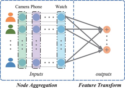
Current research focuses on developing various aggregation methods for different connection characteristics. For example, Kipf and Welling (2016) proposed local node similarity, and Donnat et al. (2018) considered structural similarity. The transformation of node features is vital for the research, such as feature cross-fusion (Feng et al., 2021) and random cover features (Zhu et al., 2020). In addition, there are many feature-related works. For example, Liu et al. (2020) proposed Deep Adaptive Graph Neural Network (DAGNN) by decoupling feature transformation and information propagation entanglement. M. Chen et al. (2020) developed an extended model of vanilla GCN that keeps input information with constant mapping. Liu et al. (2021) captured remote dependencies from node features with a non-local aggregation. X. Yang et al. (2021) proposed a self-supervised semantic aligned convolutional network (SelfSAGCN) to investigate the semantic information in features. We argue that the existing GCN approaches ignore the potential features of nodes. Although the existing GCN has an extraordinary ability to capture features, we believe that encoding potential features by a feature recommendation strategy can significantly improve the learning capability of the model. For example, we focus on the features of users' electronic purchase records: $\mathit{U}\mathit{s}\mathit{e}\mathit{r}\mathit{A}\mathit{=}\{\mathit{C}\mathit{a}\mathit{m}\mathit{e}\mathit{r}\mathit{a}\mathit{,}\mathit{P}\mathit{h}\mathit{o}\mathit{n}\mathit{e}\mathit{,}\mathit{C}\mathit{o}\mathit{m}\mathit{p}\mathit{u}\mathit{t}\mathit{e}\mathit{r}\mathit{,}\mathit{W}\mathit{a}\mathit{t}\mathit{c}\mathit{h}\}$, $\mathit{U}\mathit{s}\mathit{e}\mathit{r}\mathit{B}\mathit{=}\{\mathit{P}\mathit{h}\mathit{o}\mathit{n}\mathit{e}\mathit{,}\mathit{C}\mathit{o}\mathit{m}\mathit{p}\mathit{u}\mathit{t}\mathit{e}\mathit{r}\mathit{,}\mathit{G}\mathit{a}\mathit{m}\mathit{e}\mathit{m}\mathit{a}\mathit{c}\mathit{h}\mathit{i}\mathit{n}\mathit{e}\mathit{,}\mathit{W}\mathit{a}\mathit{t}\mathit{c}\mathit{h}\mathit{,}\mathit{D}\mathit{V}\mathit{D}\}$. After the feature recommendation, user A's most likely additional feature is the Game machine, while user B is not likely to have other features besides his own. The feature of the last two users describes as $\mathit{U}\mathit{s}\mathit{e}\mathit{r}\mathit{A}\mathit{=}\{\mathit{C}\mathit{a}\mathit{m}\mathit{e}\mathit{r}\mathit{a}\mathit{,}\mathit{P}\mathit{h}\mathit{o}\mathit{n}\mathit{e}\mathit{,}\mathit{C}\mathit{o}\mathit{m}\mathit{p}\mathit{u}\mathit{t}\mathit{e}\mathit{r}\mathit{,}\mathit{W}\mathit{a}\mathit{t}\mathit{c}\mathit{h}\mathit{,}\mathit{G}\mathit{a}\mathit{m}\mathit{e}\mathit{m}\mathit{a}\mathit{c}\mathit{h}\mathit{i}\mathit{n}\mathit{e}\}$, $\mathit{U}\mathit{s}\mathit{e}\mathit{r}\mathit{B}\mathit{=}\{\mathit{P}\mathit{h}\mathit{o}\mathit{n}\mathit{e}\mathit{,}\mathit{C}\mathit{o}\mathit{m}\mathit{p}\mathit{u}\mathit{t}\mathit{e}\mathit{r}\mathit{,}\mathit{G}\mathit{a}\mathit{m}\mathit{e}\mathit{m}\mathit{a}\mathit{c}\mathit{h}\mathit{i}\mathit{n}\mathit{e}\mathit{,}\mathit{W}\mathit{a}\mathit{t}\mathit{c}\mathit{h}\mathit{,}\mathit{D}\mathit{V}\mathit{D}\}$. As shown in Figure 2, a feature recommendation module can capture user-item interactions and opinions to obtain potential features of users and make more accurate product recommendations (Fan et al., 2019).

Figure 2. Illustration of GCN+FRS. Our proposed FRS enriches feature information by maximum possible feature recommendation and enhances the representation capability after conversion. The circles containing $\mathbf{\ast }$ indicate the recommended new features.

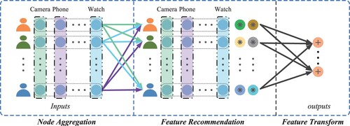
In this paper, we propose the FRS, which is inspired by the social recommender system (GraphRec) (Fan et al., 2019) and was initially proposed to solve the problem of encoding heterogeneous graphs (user social graph, user-item graph) in the social recommendation. We regard nodes and features as users and items and use a feature recommendation strategy to enhance the learning ability of the GCN model. Two methods are explicitly mentioned in the feature recommendation strategy. The first method is Maximum Possible Feature Recommendation (MPFR) means obtaining the maximum possible features of nodes with the feature recommendation module. The second is Low-Weight¹ Feature Replacement (LWFR), where the low-weight features are replaced with the maximum possible features by sorting the personalised weights of the features.

We implemented GCN+FRS performance on three citation network datasets for the node clustering task, and the experimental results demonstrate that both MPFR and LWFR methods utilised by FRS can improve the learning ability of GCN.

In summary, our contribution is twofold:

• We propose a feature recommendation strategy, including maximum possible feature recommendation and low-weight feature replacement methods, that can improve the performance of the GCN model.

• Experimentation with node classification as a learning task on three publicly available datasets demonstrates that GCN+FRS significantly outperforms SOTA methods.

Organisation of our paper The rest of our paper is organised according to the following structure. Section 2 outlines the background of graph convolutional networks and feature recommendation, respectively. Section 3 provides the necessary a priori knowledge. Section 4 summarises the overall model framework and describes each module's specifics. Section 5 reports the experimental results and experimental analysis. Section 6 concludes the paper.

2. Related work

2.1. Graph convolutional network

Graph convolutional network has become an essential tool in graph data analysis tasks, and their mainstream methods can be divided into two kinds of spatial convolution and spectral convolution. The spatial convolution-based approach defines the convolution operation on the spatial relationship of each node, learning and updating the representation from the neighbouring nodes. For example, Gilmer et al. (2017) proposed Message Passing Neural Network (MPNN) views graph convolution as a message-passing process where information can be passed directly from one node to another along an edge. Hamilton et al. (2017) suggested an inductive GraphSAGE method for transductive network representation learning. The method utilises both feature information and structure information of nodes to map graph embedding and save it, which is more scalable. Atwood and Towsley (2016) designed a propagation-convolutional neural network that adopts a matrix representation of H-hop for each node (edge or graph). Each hop represents the neighbouring information of that neighbouring range. The network can obtain local information better. Monti et al. (2017) developed a hybrid model (MoNet) that generalises the traditional CNN to non-Euclidean spaces (graphs and pops) and can learn local, smooth, combinatorial task-specific features. In addition, Veličković et al. (2017) employed an attention mechanism for the weighted summation of features of neighbouring nodes, which is used to address two critical drawbacks. The first is that the features of neighbouring nodes are closely linked to the graph's structure, limiting the model's generalisation ability. The second is that the model assigns the same weights to various neighbouring nodes in the same order.

Unlike the spatial convolution-based GCN, the spectrum-based GCN method implements the convolution operation on topological graphs through graph theory. In the first place, Bruna et al. (2013) developed a spectral convolutional neural network (Spectral CNN), but the model suffers from computational complexity, nonlocal connectivity, and too many convolutional kernel parameters to scale to large graphs. To address the above challenges, Defferrard et al. (2016) designed CheNet to reduce the computational complexity by constructing the filter as a diagonalised eigenvector approximated with Chebyshev polynomials, but the computational effort of the eigenvalue decomposition of the Laplace operator is still enormous. Then based on the previous work, Hammond et al. (2011) showed that the operator could be fitted by a Kth truncated expansion of the Chebyshev polynomial. Finally, Kipf and Welling (2016) proposed the first-order approximation of ChebNet, a simple and effective layer propagation method obtained by simplifying the computation through the first-order approximation method. The method has the advantages of weight sharing, local connectivity, and perceptual field proportional to the number of convolutional layers. In addition, some approximations to Chebyshev polynomial methods are now proposed for performing local polynomial filtering. For example, Levie et al. (2018) suggested employing Cayley polynomial approximation filters, and Liao et al. (2019) proposed multi-scale feature encoding to break the computational bottleneck of existing models.

2.2. Feature recommendation

The user-item interaction is a specific graph data in recommendation system tasks, and the utilisation of graph convolutional networks to solve recommendation problems is already a relatively common approach. We simplify the user-item interaction to two relationships, i.e. whether or not the item is owned. For recommender systems, we can regard the recommendation task as which new features the nodes are most likely to have, i.e. the recommendation system is transformed into a feature recommendation system. Berg et al. (2017) proposed a graph auto-coding framework that generates potential representations of users and items by passing distinguishable messages on the graph structure to accomplish the link prediction task. Bian et al. (2020) exploited the rumour propagation directed graph with top-down rumour propagation to learn how rumours spread and designed a diffusion propagation graph GCN with opposite directions to capture the rumour diffusion structure and learn to feature representation for rumour detection. Wu et al. (2020) suggested a novel social spammer detection model that explicitly considers three types of neighbour structures to determine the most likely features of spam. Furthermore, the feature interactions proposed by Feng et al. (2021) can also be regarded as employing existing features to combine into new features.

Notably, the heterogeneity of relationships is also the focus of the research (Chang et al., 2021). X. Wang et al. (2021) proposed a cross-view comparison mechanism for heterogeneous graph neural networks (HGNN). Zhang et al. (2019) integrated the heterogeneous structure information and the heterogeneous content information of each node to jointly learn the node representation in the heterogeneous graph. X. Wang et al. (2019) suggested an HGNN on a hierarchical attention mechanism and generates node embeddings by a hierarchical approach. There is also some other work on heterogeneous relationships (J. Hu et al., 2021; Lian & Tang, 2022). Despite the convincing success of these works, little attention has been paid to the application of feature recommendations to GCNs. In this paper, we attempt to utilise a feature recommendation strategy for generating new features of nodes, which will enhance the representation capability of GCN models.

3. Preliminary knowledge

We start by introducing some of the symbols utilised in the following sections. We denote vectors and matrices with bold lowercase letters (e.g. $\mathit{x}$) and bold uppercase letters (e.g. $\mathit{X}$). Note that all vectors are in column form without particular specification, and ${\mathit{X}}_{\mathrm{ij}}$ represents the elements of the ith row and jth column of matrix $\mathit{X}$. Finally, we use ⊙ to denote element-by-element multiplication. Some of the terms and symbols commonly used in this paper are given in Table 1.

Table 1. Symbols used in this paper.

Symbols	Descriptions
$\mathcal{G}$	a graph.
$\mathit{X}\in {\mathbb{R}}^{n\times d_0}$, $\mathit{R}\in {\mathbb{R}}^{n\times d_0}$	features matrix of a graph with N nodes.
$\mathit{A}\in {\mathbb{R}}^{n\times n}$	adjacency matrix of a graph with N nodes.
$neighbour(\mathit{x})$	neighbouring nodes of a node $\mathit{x}$.
$\mathit{N}(i)$	the set of $1\mathrm{th}$-order neighbouring nodes of a node.
$\mathcal{A}\mathcal{G}\mathcal{G}$	node aggregation function.
$\mathcal{F}\mathcal{T}$	feature transformation function.
$\mathit{W}$	weight matrix.
$\mathit{b}$	bias matrix.
$d_0,d_1,d_2,d_3$	dimension of the node representation.
$\mathit{U},\mathit{V}$	set of nodes and features.
$\mathit{O}$	set of known association relations.
$\mathcal{T}$	set of unknown association relations.
$\mathit{C}(i)$	set of features of a node.
$\mathit{B}(j)$	set of nodes containing a particular feature.
${\mathit{p}}_i\in {\mathbb{R}}^{d_0}$	embedding vector of node $u_i$.
${\mathit{q}}_j\in {\mathbb{R}}^{d_0}$	embedding vector of feature $v_j$.
$\sigma (\cdot )$	nonlinear activation function.

3.1. Graph convolutional network

A graph $\mathcal{G}$ usually consists of an adjacency matrix ($\mathit{A}\in {\mathbb{R}}^{n\times n}$) and a feature matrix ($\mathit{X}=[{\mathit{x}}_1,{\mathit{x}}_2,\dots ,{\mathit{x}}_N{]}^T\in {\mathbb{R}}^{n\times d_0}$), where n is the number of nodes and $\mathit{A}$ indicates a connection between two nodes. If ${\mathit{A}}_{ij}=1$ means an edge exists between node i and node j, otherwise, ${\mathit{A}}_{ij}=0$. $d_0$ denotes the dimensional size of the input features. The basic process of GCN is to map the input graph into the low-latitude space through the hidden layer, then learn the embedding representation of the nodes, and finally connect the output layer that performs the learning task (e.g. node classification). To simplify the notation and representation, we describe the content in terms of a single-layer GCN. As illustrated in Figure 1, the GCN performs node aggregation operation on the input and then achieves the node representation with feature transformation. The entire procedure can be described as: (1) $\begin{array}{rl}& {\mathit{x}}_{agg}=\mathcal{A}\mathcal{G}\mathcal{G}\left(\{x_n\mid n\in \mathrm{neighbour}(\mathit{x})\}\right)\\ & {\mathit{h}}_{\mathrm{out}}=\mathcal{F}\mathcal{T}\left({\mathit{x}}_{agg}\right)\end{array}$(1) where $\mathcal{A}\mathcal{G}\mathcal{G}$ denotes the aggregation function on neighbouring nodes, ${\mathit{x}}_{agg}\in {\mathbb{R}}^{d_1}$ indicates the potential features of the node as a result of the $\mathcal{A}\mathcal{G}\mathcal{G}$ operation, $\mathcal{F}\mathcal{T}$ represents the feature transformation function, and ${\mathit{h}}_{\mathrm{out}}\in {\mathbb{R}}^{d_2}$ is the final obtained rich representation of the target node.

3.1.1. Node aggregation

Node aggregation is to update the information of the target node by aggregating that of the neighbouring nodes. The basic principle is that neighbouring node feature information reflects that of the target node. For example, in a citation network, a target paper with cross-citation relationships with multiple papers in a field may be in the same field. Notice that $\mathrm{neighbour}(\mathit{x})$ can contain self-connections (form $\mathit{x}$ to $\mathit{x}$), and sampling can fetch all neighbouring nodes (Kipf & Welling, 2016) or a fixed number of random neighbouring nodes (Hamilton et al., 2017). Furthermore, different $\mathcal{A}\mathcal{G}\mathcal{G}$ methods capture different information about neighbouring nodes (Duan et al., 2021; Hamilton et al., 2017; Kipf & Welling, 2016; Xu et al., 2018), such as obtaining common attributes of nodes filtered by a fixed number of neighbouring average pools, and maximum pools obtain the most salient features among nodes.

3.1.2. Feature transformation

Feature transformation is an operation to obtain a potentially rich representation by projecting the target node features into the high-latitude space. Existing GCNs usually adopt nonlinear activation mappings: (2) ${\mathit{h}}_{\mathrm{out}}=\mathcal{F}\mathcal{T}(\mathit{x})=\sigma (\mathit{W}\mathit{x}+\mathit{b})$(2) where $\mathit{W}\in {\mathbb{R}}^{d_2\times d_0}$ represents the weight matrix, $\mathit{b}\in {\mathbb{R}}^{d_2}$ denotes the bias vector, and σ indicates the activation function.

3.2. Feature recommendation

We employ the adjacency matrix and the feature matrix as inputs to the feature recommendation module to predict the maximum possible features of the nodes. Let $\mathit{U}=\{u_1,u_2,\dots ,u_n{\}}^T$ and $\mathit{V}=\{v_1,v_2,\dots ,v_m{\}}^T$ represent the set of nodes and features, respectively, where m and n denote the number of features and nodes. Assume that $\mathit{R}\in {\mathbb{R}}^{n\times m}$ denotes the association matrix of nodes and features (i.e. the feature matrix $\mathit{X}$). Here we define the association relationship with $r_{ij}$. Specifically, if $v_j$ is a feature of $u_i$, then $r_{ij}=1$, otherwise, $r_{ij}=0$. Suppose $O=\{⟨u_i,v_j⟩\mid r_{ij}=0\mathrm{or}{r}_{ij}=1\}$ is the set of known association relations and $\mathcal{T}=\{⟨u_i,v_j⟩\mid r_{ij}\notin O\}$ denotes the set of unknown association relations. Let $\mathit{N}(i)$ be the set of first-order neighbouring nodes of $u_i$, $\mathit{C}(i)$ is the set of features of $u_i$, and $\mathit{B}(j)$ represents the set of nodes containing feature $v_j$. Furthermore, the adjacency matrix is expressed with $\mathit{A}\in {\mathbb{R}}^{n\times n}$. ${\mathit{A}}_{ij}=1$ if there is a relationship between two nodes $u_i$ and $u_j$, otherwise ${\mathit{A}}_{ij}=0$. Knowing the feature matrix $\mathit{R}$ and the adjacency matrix $\mathit{A}$, we aim to predict the potential features of each node and obtain the maximum possible features of the nodes. Also, we represent node $u_i$ with embedding vector ${\mathit{p}}_i\in {\mathbb{R}}^{d_0}$ and feature $v_j$ with embedding vector ${\mathit{q}}_j\in {\mathbb{R}}^{d_0}$.

4. Feature recommendation strategy for graph convolutional network

This section begins with a general introduction to the FRS framework, followed by detailed descriptions of the feature recommendation module and the low-weight feature replacement module, respectively, and finally explains how the GCN module performs feature learning.

4.1. Overview of our proposed framework

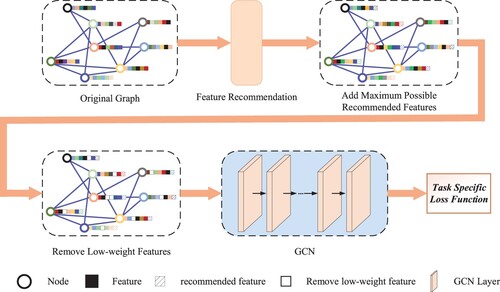
The framework of our proposed model is illustrated in Figure 3, which consists of three modules: feature recommendation module, low-weight feature replacement module, and GCN module. The first module is feature recommendation, i.e. recommending the potential features of each node. Since the recommendation module has two different inputs (adjacency matrix and feature matrix), we will learn the representation of nodes from different perspectives. The second module primarily completes the low-weight feature replacement. After the association weights between nodes and features are obtained from the recommendation module, we use the maximum possible recommended features to replace the features of low-weight connections. Finally, there is the GCN module, where we input the original adjacency and the processed feature matrices, learn the representation of the nodes, and complete the final classification task.

Figure 3. The overall framework of our proposed model.

4.2. Feature recommendation module

The overall structure of the feature recommendation module is illustrated in Figure 4, which consists of three components: node modelling, feature modelling, and relationship prediction. The first part is node modelling, i.e. learning the latent factors of the nodes. Since the input contains two different matrices (adjacency matrix and feature matrix), we will learn the representation of the nodes from two perspectives. Therefore, two aggregation operations are introduced to handle the corresponding matrix inputs. One is feature aggregation, which understands nodes by feature matrix. That is, whether there is an association relationship between nodes and features. The other is neighbour aggregation, the relationship between nodes and nodes. It can help us model a node from the perspective of its neighbour relationship. The second component is feature modelling, which is learning about the potential factors of features. Having already understood the nodes from the feature perspective, we modelled the features from the node perspective (which nodes are a feature owned by) to thoroughly understand the connection between nodes and features. The final component integrates the previous two components to learn the model parameters through feature prediction. We will describe each component in detail below.

Figure 4. The overall structure of the feature recommendation module. Node modelling, feature modelling, and feature prediction are the three main components.

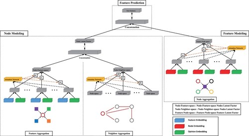
4.2.1. Node modelling

The purpose of node modelling is to learn the potential factors of nodes, and the challenge is to figure out how to combine the adjacency matrix and the feature matrix to represent node $u_i$ as ${\mathit{h}}_i\in {\mathbb{R}}^{d_3}$. To better learn the node representation, we designed two types of aggregation operations: feature aggregation and neighbour aggregation. As shown in the left part of Figure 4, feature aggregation learns the potential representation of nodes ${\mathit{h}}_i^F\in {\mathbb{R}}^{d_4}$ through the feature matrix, while neighbour aggregation is learning the potential representation of nodes ${\mathit{h}}_i^A\in {\mathbb{R}}^{d_4}$ through the adjacency matrix. Then the potential representation ${\mathit{h}}_i$ is obtained by combining the two representations. The following section will detail feature aggregation, neighbour aggregation, and how to learn the representation of nodes from the adjacency matrix and feature matrix.

4.2.1.1 A. Feature aggregation

We provide a principled approach for learning latent user factors ${\mathit{h}}_i^F$ in the node-feature-space by capturing the interaction of nodes and features in the feature matrix. The purpose of feature aggregation is to learn the latent user factors ${\mathit{h}}_i^F$ in the node-feature-space by the features of the user $u_i$. The following function represents this aggregation: (3) ${\mathit{h}}_i^F=\sigma (\mathit{W}\cdot {\mathcal{A}\mathcal{G}\mathcal{G}}_{\mathrm{feature}}\left(\{{\mathit{x}}_{ia},\mathrm{\forall }a\in C(i)\}\right)+\mathit{b})$(3) where $C(i)$ indicates the feature set of node $u_i$, ${\mathit{x}}_{ia}$ denotes the representation vector of the association relationship between node $u_i$ and feature $v_a$, and ${\mathcal{A}\mathcal{G}\mathcal{G}}_{\mathrm{feature}}$ is the aggregation operation. $\sigma (\cdot )$ represents the nonlinear activation function. $\mathit{W}$ denotes the trainable weight matrix, and $\mathit{b}$ indicates the trainable bias matrix. In the following, we will describe how to define the association relation ${\mathit{x}}_{ia}$ and the aggregation function ${\mathcal{A}\mathcal{G}\mathcal{G}}_{\mathrm{feature}}$.

The association relationship between nodes and features is indicated as r. The preference of nodes for features can be captured through the association relationship, which helps model the potential factors in the node-feature-space. To model the association relationship, we introduce an embedding vector ${\mathit{e}}_r\in {\mathbb{R}}^{d_0}$ for the two association relationships (associated and unassociated). We first combine the feature representation ${\mathit{q}}_a$ and association relation representation ${\mathit{e}}_r$ for the interactions between nodes $u_i$, feature $v_a$, and association relation r, followed by a multilayer perceptron (MLP) to obtain the feature interaction representation ${\mathit{x}}_{ia}$. The mathematical representation can be described as follows: (4) ${\mathit{x}}_{ia}=g_v\left([{\mathit{q}}_a\oplus {\mathit{e}}_r]\right)$(4) where ⊕ represents the union of two vectors and $g_v$ indicates the fusion function.

${\mathcal{A}\mathcal{G}\mathcal{G}}_{\mathrm{feature}}$ was initially considered with mean aggregation, i.e. taking the mean of all $\{{\mathit{x}}_{ia},\mathrm{\forall }a\in C(i)\}$ vector elements. This aggregator is similar to the first-order linear approximation of a local convolution (Kipf & Welling, 2016) and can be expressed as: (5) ${\mathit{h}}_i^F=\sigma (\mathit{W}\cdot \left\{\sum _{a\in C(i)}{\alpha }_i{\mathit{x}}_{ia}\right\}+\mathit{b})$(5) where the size of ${\alpha }_i$ is equal to $\frac{1}{|C(i)|}$. In this aggregator, all feature interactions contribute equally to the node $u_i$. However, this approach is not optimal for node understanding, so we need to assign different weights to each interaction to represent the different contributions to the potential factors of the node.

Different weights need to be assigned for different interactions. We generate the feature attention ${\alpha }_{ia}$ with a multilayered neural network, called attention network, i.e. assigning a personalised weight to each $(v_a,u_i)$. Equation (5(5) ${\mathit{h}}_i^F=\sigma (\mathit{W}\cdot \left\{\sum _{a\in C(i)}{\alpha }_i{\mathit{x}}_{ia}\right\}+\mathit{b})$(5) ) can be rewritten as follows: (6) ${\mathit{h}}_i^F=\sigma (\mathit{W}\cdot \left\{\sum _{a\in C(i)}{\alpha }_{ia}{\mathit{x}}_{ia}\right\}+\mathit{b})$(6) For attention networks, the inputs are the interacting association relations ${\mathit{x}}_{ia}$ and the embedding representations of the nodes ${\mathit{p}}_i$. Attention network can be defined formally as: (7) ${\alpha }_{ia}^{\ast }={\mathit{w}}_2^T\cdot \sigma ({\mathit{W}}_1\cdot [{\mathit{x}}_{ia}\oplus {\mathit{p}}_i]+{\mathit{b}}_1)+{\mathit{b}}_2$(7) Finally, the attention weights are normalised by the softmax function and the potential factor contribution of the association relationship to node $u_i$ in the node-feature-space is obtained as: (8) ${\alpha }_{ia}=\frac{\exp \left({\alpha }_{ia}^{\ast }\right)}{\sum _{a\in C(i)}\exp \left({\alpha }_{ia}^{\ast }\right)}$(8)

4.2.1.2 B. Neighbour aggregation

The feature preferences are similar to that of its neighbouring nodes, so we will combine the information of neighbouring nodes to obtain rich potential factors for the user. Therefore, we introduce an attention mechanism to aggregate the information of neighbouring nodes. To understand the nodes from their interactions, we will employ the adjacency matrix to aggregate the potential factors of neighbouring nodes. In the node-adjacency-space, the potential factor ${\mathit{h}}_i^A$ of node $u_i$ is formed by aggregating the neighbouring nodes $N(i)$. The specific function is described as follows: (9) ${\mathit{h}}_i^A=\sigma (\mathit{W}\cdot {\mathcal{A}\mathcal{G}\mathcal{G}}_{\mathrm{neighbours}}\left(\{{\mathit{h}}_o^F,\mathrm{\forall }o\in N(i)\}\right)+\mathit{b})$(9) where ${\mathcal{A}\mathcal{G}\mathcal{G}}_{\mathrm{neighbours}}$ represents the aggregation operation of neighbouring nodes.

The ${\mathcal{A}\mathcal{G}\mathcal{G}}_{\mathrm{neighbours}}$ function is the first to adopt the mean aggregation, which performs the mean operation on the elements of the vector in $\{{\mathit{h}}_o^F,\mathrm{\forall }o\in N(i)\}$. The function can be expressed as: (10) ${\mathit{h}}_i^A=\sigma (\mathit{W}\cdot \left\{\sum _{o\in N(i)}{\beta }_i{\mathit{h}}_o^F\right\}+\mathit{b})$(10) where ${\beta }_i$ is fixed as $\frac{1}{|N(i)|}$. The mean aggregator assumes all neighbouring nodes contribute to the target node. However, this method is likewise not optimal, so we also apply the exact attention mechanism to generate personalised weights indicating the importance of different neighbouring nodes to $u_i$. The related function can be expressed as follows: (11) $\begin{array}{rl}{\mathit{h}}_i^A& =\sigma (\mathit{W}\cdot \left\{\sum _{o\in N(i)}{\beta }_{io}{\mathit{h}}_o^F\right\}+\mathit{b})\\ {\beta }_{io}^{\ast }& ={\mathit{w}}_2^T\cdot \sigma ({\mathit{W}}_1\cdot [{\mathit{h}}_o^F\oplus {\mathit{p}}_i]+{\mathit{b}}_1)+b_2\\ {\beta }_{io}& =\frac{\exp \left({\beta }_{io}^{\ast }\right)}{\sum _{o\in N(i)}\exp \left({\beta }_{io}^{\ast }\right)}\end{array}$(11) where ${\beta }_{io}^{\ast }$ represents the personalisation weight of neighbouring nodes.

4.2.1.3 C. Learning node latent factor

To learn the potential representations of nodes more effectively, we need to consider both the potential representations of users in the node-feature-space and the potential representations of users in the node-neighbour-space. We utilise MLP to combine the two potential representations as to the potential representation of the final node, where the potential representation of the node feature space is ${\mathit{h}}_i^F$ and the potential representation of the node neighbour space is ${\mathit{h}}_i^A$. Therefore, the potential representation ${\mathit{h}}_i$ of the node can be defined as: (12) $\begin{array}{rl}{\mathit{c}}_1& =[{\mathit{h}}_i^F\oplus {\mathit{h}}_i^A]\\ {\mathit{c}}_2& =\sigma ({\mathit{W}}_2\cdot {\mathit{c}}_1+{\mathit{b}}_2)\\ & \cdots \\ {\mathit{h}}_i& =\sigma ({\mathit{W}}_l\cdot {\mathit{c}}_{l-1}+{\mathit{b}}_l)\end{array}$(12) where l indicates the serial number of the hidden layer.

4.2.2. Feature modelling

As illustrated on the right side of Figure 4, feature modelling is utilised to achieve a potential representation ${\mathit{Z}}_j$ of feature $v_j$ in the feature-node-space by aggregating the nodes. We learn the potential representations of features by capturing the interactions of nodes with features in the feature matrix. For each feature $v_j$, we need to capture information from the set of nodes interacting with $v_j$, denoted as $B_j$.

There are different association relations with different nodes, even for the same feature. We use MLP to fuse the combination of the node representation ${\mathit{p}}_t$ and the association relation representation ${\mathit{e}}_r$. The fusion function is denoted as $g_u$. The function can be expressed as: (13) ${\mathit{f}}_{jt}=g_u\left([{\mathit{p}}_t\oplus {\mathit{e}}_r]\right)$(13) where ${\mathit{f}}_{jt}$ denotes the interaction relationship. Then, we attempt to aggregate the interaction information of nodes in $B_j$ for the feature $v_j$. The aggregation function of nodes is denoted as ${\mathcal{A}\mathcal{G}\mathcal{G}}_{nodes}$ for aggregating the interactions of nodes $\{{\mathit{f}}_{jt},\mathrm{\forall }t\in B(j)\}$, and finally, the potential representation of features ${\mathit{z}}_j$ can be defined as: (14) ${\mathit{z}}_j=\sigma (\mathit{W}\cdot {\mathcal{A}\mathcal{G}\mathcal{G}}_{\mathrm{nodes}}\left(\{{\mathit{f}}_{jt},\mathrm{\forall }t\in B(j)\}\right)+\mathit{b})$(14) Similarly, we apply the attention method and utilise a multilayer neural network to acquire the personalised weights of each node for the features. With ${\mathit{f}}_{jt}$ and ${\mathit{q}}_j$ as inputs, the process can be expressed as: (15) $\begin{array}{rl}{\mathit{z}}_j& =\sigma (\mathit{W}\cdot \left\{\sum _{t\in B(j)}{\mu }_{jt}{\mathit{f}}_{jt}\right\}+\mathit{b})\\ {\mu }_{jt}^{\ast }& ={\mathit{w}}_2^T\cdot \sigma ({\mathit{W}}_1\cdot [{\mathit{f}}_{jt}\oplus {\mathit{q}}_j]+{\mathit{b}}_1)+b_2\\ {\mu }_{jt}& =\frac{\exp \left({\mu }_{jt}^{\ast }\right)}{\sum _{t\in B_{(j)}}\exp \left({\mu }_{jt}^{\ast }\right)}\end{array}$(15) where ${\mu }_{jt}$ denotes the personalised impact of different nodes on the potential representation of the learned features.

4.2.3. Feature recommendation module training

After acquiring potential representations of nodes and features, we will use feature prediction to learn the model's parameters. We first connect the two potential representations ($[h_i\oplus z_j]$) and then input them to the MLP for the feature prediction task. The specific process can be expressed as follows: (16) $\begin{array}{rl}{\mathit{g}}_1& =[{\mathit{h}}_i\oplus {\mathit{z}}_j]\\ {\mathit{g}}_2& =\sigma ({\mathit{W}}_2\cdot {\mathit{g}}_1+{\mathit{b}}_2)\\ & \cdots \\ {\mathit{r}}_{ij}^{\mathrm{\prime }}& ={\mathit{w}}^T\cdot {\mathit{g}}_{l-1}\end{array}$(16) where l denotes the serial number of the hidden layer, ${\mathit{r}}_{ij}^{\mathrm{\prime }}$ represents the association between node $u_i$ and feature $v_j$. Finally, the new association relations form a new feature matrix, each row representing a new feature of the node.

4.2.4. Feature prediction

To determine the parameters of the feature recommendation module, we use Euclidean distance as the loss function for training. The loss function can be described as follows: (17) $Loss=\frac{1}{2|O|}\sum _{i,j\in O}{(r_{ij}^{\mathrm{\prime }}-r_{ij})}^2$(17) where $|O|$ represents the number of association relations between nodes and features, and $r_{ij}$ is the true association relation between node $u_i$ and feature $v_j$.

To optimise the objective function of the feature recommendation module, we employ Adam (Kingma & Ba, 2014) as an optimiser in practice. In the model training phase, we randomly initialise three embedding representations, including the embedding representation ${\mathit{q}}_j$ of nodes, the embedding representation ${\mathit{p}}_i$ of features, and the embedding representation ${\mathit{e}}_r$ of association relations. It is worth noting that the size of ${\mathit{e}}_r$ depends on the complexity of the relationship between features and nodes. For example, whether nodes and features are associated with each other, ${\mathit{e}}_r$ uses two different embedding vectors to represent $\{0,1\}$. In addition, to prevent the problem of overfitting, we adopt the dropout strategy (Srivastava et al., 2014).

4.3. Low-weight feature replacement module

To obtain a richer feature representation, we model the nodes and features separately with two aggregation operations in the feature recommendation module and finally achieve the maximum possible recommended features that exceed the threshold value by relationship prediction. Meanwhile, personalised weights for the influence of each node on the features can also be available during the training process.

With these considerations, we try to use the maximum possible recommended features to replace the low-weight features of the nodes. We divide the process into two steps: the first is to add the maximum possible recommendation features for each node; the second is to remove the same number of low-weight features.

4.4. GCN module and classification learning tasks

We adopt the model proposed by Kipf and Welling (2016) in the GCN module, assuming that $\mathit{A}\in {\mathbb{R}}^{n\times n}$ denotes the adjacency matrix and $\mathit{X}\in {\mathbb{R}}^{n\times d_0}$ represents the feature matrix, then its propagation rule can be described as: (18) $\begin{array}{rl}{\mathit{H}}^{(l+1)}& =\sigma \left({\tilde{\mathit{D}}}^{-\frac{1}{2}}\tilde{\mathit{A}}{\tilde{\mathit{D}}}^{-\frac{1}{2}}{\mathit{H}}^{(l)}{\mathit{W}}^{(l)}\right),l=0,1\dots \\ {\mathit{H}}^{(0)}& =\mathit{X}\end{array}$(18) where $\sigma (\cdot )$ denotes a nonlinear activation function. ${\mathit{H}}^{(l)}\in {\mathbb{R}}^{n\times d_l}$ represents the $(l-1)\mathrm{th}$ hidden layer's output and the $l\mathrm{th}$ hidden layer's input. ${\mathit{W}}^{(l)}\in {\mathbb{R}}^{d_l\times d_{l+1}}$ denotes the trainable parameter matrix. The matrix ${\tilde{\mathit{D}}}^{-\frac{1}{2}}\tilde{\mathit{A}}{\tilde{\mathit{D}}}^{-\frac{1}{2}}$ denotes the normalisation of the convolution matrix ${\mathit{I}}_n+{\mathit{D}}^{-\frac{1}{2}}{\mathit{A}\mathit{D}}^{-\frac{1}{2}}$, where ${\mathit{I}}_n$ denotes the unit matrix, and $\mathit{D}$ denotes the degree matrix.

According to Kipf and Welling (2016) the best implementation is obtained by stacking two layers of GCN. As shown in Equation (19(19) $\begin{array}{rl}{\mathit{H}}^{(1)}& =\mathrm{ReLU}\left({\tilde{\mathit{D}}}^{-\frac{1}{2}}\tilde{\mathit{A}}{\tilde{\mathit{D}}}^{-\frac{1}{2}}\mathit{X}{\mathit{W}}^{(0)}\right)\\ {\mathit{H}}^{(2)}& =\mathrm{softmax}\left({\tilde{\mathit{D}}}^{-\frac{1}{2}}\tilde{\mathit{A}}{\tilde{\mathit{D}}}^{-\frac{1}{2}}{\mathit{H}}^{(1)}{\mathit{W}}^{(1)}\right)\end{array}$(19) ). (19) $\begin{array}{rl}{\mathit{H}}^{(1)}& =\mathrm{ReLU}\left({\tilde{\mathit{D}}}^{-\frac{1}{2}}\tilde{\mathit{A}}{\tilde{\mathit{D}}}^{-\frac{1}{2}}\mathit{X}{\mathit{W}}^{(0)}\right)\\ {\mathit{H}}^{(2)}& =\mathrm{softmax}\left({\tilde{\mathit{D}}}^{-\frac{1}{2}}\tilde{\mathit{A}}{\tilde{\mathit{D}}}^{-\frac{1}{2}}{\mathit{H}}^{(1)}{\mathit{W}}^{(1)}\right)\end{array}$(19) where ${\mathit{W}}^{(0)}\in {\mathbb{R}}^{d_0\times d_1}$ and ${\mathit{W}}^{(1)}\in {\mathbb{R}}^{d_1\times d_2}$ are trainable weight matrices of the corresponding hidden layers. $\mathrm{ReLU}(\cdot )$ and $\mathrm{softmax}(\cdot )$ denote the two activation functions. Furthermore, let the actual label set be $\mathit{Y}\in {\mathbb{R}}^{n\times f}$, defined as ${\mathit{Y}}_{ij}=1$ if the label of node i is j, otherwise ${\mathit{Y}}_{ij}=0$. The cross-entropy loss defines the classification error of the training: (20) ${\mathcal{L}}_{\mathrm{class}}=-\frac{1}{n}\sum _{i=1}^n\sum _{j=1}^f{Y}_{ij}\log H_{ij}^{(2)}$(20)

5. Experiments

In this section, we first evaluate the effectiveness of the FRS on three publicly available datasets, then analyse the model's performance from different perspectives, and finally demonstrate the portability and generalisation ability of the strategy.

5.1. Datasets

Citation networks are documents and the relationships between them, nodes represent documents, tags indicate the topics of documents, features are the bags of words contained in the content of documents, and edges denote the cross-references between documents. We tested the proposed strategy on three citation network datasets, including Cora (McCallum et al., 2000), Citeseer (Giles et al., 1998) and Pubmed (Sen et al., 2008). The details of the three citation network datasets are as follows:

• Cora contains 2708 nodes and 5249 edges. All nodes are divided into seven classes, and each node has a 1433-dimensional feature vector.

• Citeseer contains 3327 nodes and 4732 edges. All nodes are divided into six classes, and each node has 3707-dimensional feature vectors.

• Pubmed is a relatively large citation network, containing 19,717 nodes and 44,338 edges. All nodes are divided into three classes, and each node has a 500-dimensional feature vector.

5.2. Baseline

Since we focus only on the feature aspect of modelling, we will ignore baselines based on node aggregation modelling, such as GAT (Veličković et al., 2017), DCNN (Atwood & Towsley, 2016) and DAGNN (Liu et al., 2020). The more advanced baselines are listed below:

• SemiEmb (Weston et al., 2012) utilises a graph learning method based on Laplace regularisation.

• DeepWalk (Perozzi et al., 2014) is a method for learning graph representations with skip-gram techniques, where node representations are learned by performing random walks through the generated node contexts.

• GCN (Kipf & Welling, 2016) performs feature transformation through matrix mapping and aggregation of nodes through the pooling function.

• GIN (Xu et al., 2018) is a generalisation of vanilla GCN with feature transformation with MLP in each convolutional layer.

• Cross-GCN (Feng et al., 2021) learns the hidden representation of nodes by modelling the intersection features.

• GCN+RCF (Zhu et al., 2020) improves the feature learning capability of GCN by adopting the strategy of randomly covering features.

• SelfSAGCN (X. Yang et al., 2021) learns nodes with the same label from both semantic and graph structure perspectives, respectively, and aligns node features with a class-centred acquaintance.

5.3. Setup

Our implementation of GCN+FRS and SelfSAGNC+FRS uses Pytorch² and adopts the public code of GCN³ and SelfSAGCN.⁴ To illustrate the effectiveness of both MPFR and LWFR methods in the recommended strategy, we employed the best parameters of GCN (Kipf & Welling, 2016) from the original paper.

In the GCN module, We set the value of the deactivation rate to 0.5 and weights decay to $5\mathrm{e}-4$. In the feature recommendation module, we dedicate $90\mathrm{\%}$ of the node features to training, and then $10\mathrm{\%}$ of the features are applied to test the effect of the model. In addition, we set the batch size to 128, and the relationship between nodes and features is represented with 16 bits. Notably, the threshold value is 0.9. i.e. a predicted relationship value between nodes and features above 0.9 indicates that the node has this feature. Due to the sparsity of the features, we group positive samples with an equal number of randomly sampled negative samples into a sample_set, which is employed to keep the balance of negative and positive samples during the training procedure by sample set. The model works best when the sample_set value is 12. Adam (Kingma & Ba, 2014) optimises both the feature recommendation and GCN modules, and the initial learning rates are set to 0.01.

5.4. Experimental analysis

We first test the effect of both MPFR and LWFR methods on the model, then compare the model performance with the SOTA method, and finally analyse the effect of different parameters on the model performance. In addition, to illustrate the model's effectiveness, we run our method through 20 random trials and report the average performance and margin of error.

5.4.1. Impact of the two methods

To test the model performance improvement by the MPFR method and the LWFR method, we evaluated different scenarios on the Cora data: using MPFR alone and a mixture of the two methods.

Table 2 summarises the results of GCN performing the node classification task after using different recommendation strategies on the Cora dataset. We can observe from the results that the use of MPFR alone and a mixture of both methods (MPFR & LWFR) can improve the performance of GCN. After comparing the maximum and average values of the classification results, it can be concluded that the recommendation strategy with a mixture of the two methods allows the model to obtain better performance compared to using MPFR alone.

Table 2. The performance of GCN in two scenarios.

Sample_set	GCN	ACC(%)
	without	81.5
$1\sim 5$	MPFR	83.1 (82.6)
	MPFR & LWFR	83.1 (82.8)
$6\sim 10$	MPFR	83.0 (82.9)
	MPFR & LWFR	83.3 (83.1)
$11\sim 15$	MPFR	83.1 (83.0)
	MPFR & LWFR	83.4 (83.2)
$16\sim 20$	MPFR	82.9 (82.6)
	MPFR & LWFR	82.9 (82.6)
$21\sim 25$	MPFR	82.7 (82.6)
	MPFR & LWFR	82.9 (82.5)
$26\sim 30$	MPFR	82.4 (82.3)
	MPFR & LWFR	82.9 (82.7)

Note: Outside the parentheses are the maximum values, while inside the parentheses are the average values.

5.4.2. Performance comparison

After applying FRS from the recommendation strategy to the GCN and SelfSAGCN, Table 3 reports the model's performance on the three citation network datasets. It is clear from Table 3 that our proposed recommended strategy improves the performance of GCN by about $1.6\mathrm{\%}$, $0.4\mathrm{\%}$, and $0.4\mathrm{\%}$, respectively. In addition, we use FRS for the latest GCN method, SelfSAGCN, and SelfSAGCN+FRS achieves the most advanced performance compared to other improved feature methods.

Table 3. Summary of results for classification accuracy on three databases.

Model	Cora(%)	Pubmed(%)	Citeseer(%)
SemiEmb (Weston et al., 2012)	59.0	71.1	59.6
DeepWalk (Perozzi et al., 2014)	67.2	65.3	43.2
GCN+RCF (Zhu et al., 2020)	82.7	–	–
GIN (Xu et al., 2018)	$78.5\pm 1.9$	$78.7\pm 1.6$	$68.9\pm 2.0$
GCN (Kipf & Welling, 2016)	$79.1\pm 1.8$	$77.6\pm 2.0$	$69.7\pm 2.0$
Cross-GCN (Feng et al., 2021)	$78.9\pm 1.6$	$79.3\pm 1.8$	$71.3\pm 1.7$
SelfSAGCN (X. Yang et al., 2021)	$83.8\pm 0.5$	$80.7\pm 1.5$	$73.5\pm 1.2$
GCN+FRS	$81.4\pm 2.0$	$79.9\pm 1.6$	$71.6\pm 2.0$
SelfSAGCN+FRS	$\mathbf{84.1}\pm 0.9$	$\mathbf{81.3}\pm 1.3$	$\mathbf{73.8}\pm 1.6$

5.4.3. Effect of embedding size

We test the impact of different model complexity on the recommendation effect by representing embeddings of different sizes, and Figure 5 shows the results of the performance tests on the Cora dataset. The embedding representation size of the recommended module in the test is set to $\mathrm{E}=[8,16,32,64,128]$ and keeps the maximum possible features to be updated at around 500. According to the experimental results, we can get the below conclusions:

Figure 5. Effect of embedding size. GCN+FRS1 denotes a single MPFR method operating on GCN, whereas GCN+FRS2 represents a combination of MPFR and LWFR methods working on GCN.

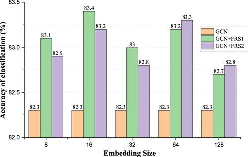
• In all cases, the model's performance with the recommended strategy is significantly better than that of the GCN alone. It further illustrates the effectiveness of our proposed recommendation strategy.

• In addition, GCN+FRS (GCN+FRS2) with $\mathrm{E}=16$ exhibits exciting performance, consistently outperforming embedded representations with other sizes.

5.4.4. Different number of sample_set

This subsection tests the effect of different numbers of sample sets on model performance. Figure 6 shows the classification task on the Cora dataset with a different number of sample sets. From the results observed, we obtain the following conclusions:

Figure 6. Different number of simple_set. GCN+FRS1 denotes a single MPFR method operating on GCN, whereas GCN+FRS2 represents a combination of MPFR and LWFR methods working on GCN.

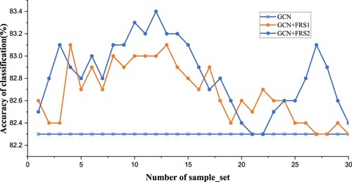
• Overall, better performance is obtained with the recommended policy than without it. The effectiveness of the recommended policy is illustrated from this perspective.

• The model performed best on the Cora dataset when the value of the simple_set equals 12.

• From the results of the classification task, the performance generally shows an increasing trend as the simple_set increases from 1 to 12, but after exceeding 12 (Less than 19), the performance starts to decrease.

We tested the prediction of the feature matrix using the recommendation module alone with a correct rate of $74.1\mathrm{\%}$. From the results, we can see noise in the predicted features. When the correct number of recommended features is obtained, the positive impact of the recommendation strategy on the classification results outweighs the negative impact, and conversely, when the number of recommended features exceeds a specific value, the result is the opposite.

5.4.5. Hyperparametric analysis

We also investigated the effect of hyperparameters on the recommendation effectiveness of the recommendation module. We have chosen the dropout parameter as an example to illustrate that this parameter affects the results of the classification task by influencing the recommended features. Figure 7 shows the effect of the parameters on the model's performance when increasing the dropout from 0.1 to 0.7 on the Cora dataset. From the results, we have the following analysis:

Figure 7. Hyperparametric analysis. GCN+FRS1 denotes a single MPFR method operating on GCN, whereas GCN+FRS2 represents a combination of MPFR and LWFR methods working on GCN.

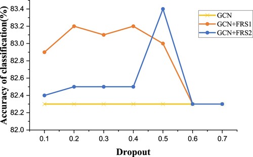
• After the dropout value is more significant than 0.5, the recommendation module does not obtain the maximum possible characteristics of the node.

• The best performance of the GCN+FRS model is obtained when dropout value is equal to 0.5 (GCN+FRS2). This result is reasonable since the most randomly generated network structures are available in this condition.

• GCN+FRS1 performs more consistently than GCN+FRS2. This is that GCN+FRS1 solely employs the MPFR method, which keeps each node's original features, but GCN+FRS2 combines MPRF and LWFR methods to replace original features with predicted features. The noise affects the classification task results when too many features are replaced.

5.5. Portability and generalisability

We experiment on another representative model, GAT, to test our proposed recommendation strategy's portability and generalisation ability. The experiment results are shown in Table 4.

Table 4. Summary of results for classification accuracy on three databases.

Model	Cora(%)	Citeseer(%)	Pubmed(%)
GAT (Veličković et al., 2017)	$83.0\pm 0.7$	$72.5\pm 0.7$	$79.0\pm 0.3$
GAT+FRS1	$83.5\pm 0.6$	$72.7\pm 0.9$	$\mathbf{79.3}\pm 0.6$
GAT+FRS2	$\mathbf{83.6}\pm 0.7$	$\mathbf{72.9}\pm 1.1$	$79.2\pm 0.9$

As we can see in Table 4, the feature recommendation strategy also improves the performance of the GAT model, demonstrating the portability and generalisation ability of the recommendation strategy.

5.6. Limitations

In this section, we describe several limitations of the proposed model.

Rich information on node and feature interactions The current model understands the interaction between a node and a feature as $\{0,1\}$, i.e. whether the node possesses the feature or not. However, the interaction relationships in real datasets are rich in correlations. For example, in the citation network dataset, each paper is represented by the bag of words it contains while ignoring other information such as the frequency of the bag of words.

Feature-to-feature interaction The current model only focuses on three interactions: node-to-node, node-to-feature, and feature-to-node, but feature-to-feature should also have similar interactions to those between nodes. Feature-to-feature interaction can achieve feature recommendation with better performance.

6. Conclusion

In this paper, we proposed a feature recommendation strategy (FRS) for graph convolutional networks. It provides two feature recommendation strategies, maximum possible feature recommendation and low-weight feature replacement, for updating node features and improving the performance of the GCN model. Experiments are conducted on three datasets, and the results demonstrate the effectiveness, portability, and generalisability of the recommendation strategy. In the future, we will discuss how to integrate feature recommendation methods into different heterogeneous graph neural frameworks to achieve better messaging and generate more effective patient representations.

Disclosure statement

No potential conflict of interest was reported by the author(s).

Additional information

Funding

This work was supported by the Postgraduate Research & Practice Innovation Program of Jiangsu Province (KYCX21_0408).

Notes

1 In this paper, low-correlation and low-weight mean the same thing, and we use them mixed.

2 https://pytorch.org

3 https://github.com/tkipf/pygcn

4 https://github.com/xdxuyang/SelfSAGCN

References

- Atwood, J., & Towsley, D. (2016). Diffusion-convolutional neural networks. In Advances in neural information processing systems (Vol. 29). Curran Associates, Inc.
- Berg, R. V. D., Kipf, T. N., & Welling, M. (2017). Graph convolutional matrix completion. arXiv preprint arXiv:1706.02263. https://doi.org/10.48550/arXiv.1706.02263
- Bian, T., Xiao, X., Xu, T., Zhao, P., Huang, W., Rong, Y., & Huang, J. (2020). Rumor detection on social media with bi-directional graph convolutional networks. Proceedings of the AAAI Conference on Artificial Intelligence, 34(1), 549–556. https://doi.org/10.1609/aaai.v34i01.5393
- Bruna, J., Zaremba, W., Szlam, A., & LeCun, Y. (2013). Spectral networks and locally connected networks on graphs. arXiv preprint arXiv:1312.6203. https://doi.org/10.48550/arXiv.1312.6203
- Chang, F., Ge, L., Li, S., Wu, K., & Wang, Y. (2021). Self-adaptive spatial-temporal network based on heterogeneous data for air quality prediction. Connection Science, 33(3), 427–446. https://doi.org/10.1080/09540091.2020.1841095
- Chen, J., Pan, L., Wei, Z., Wang, X., Ngo, C. W., & Chua, T. S. (2020). Zero-shot ingredient recognition by multi-relational graph convolutional network. Proceedings of the AAAI Conference on Artificial Intelligence, 34(7), 10542–10550. https://doi.org/10.1609/aaai.v34i07.6626
- Chen, M., Wei, Z., Huang, Z., Ding, B., & Li, Y. (2020). Simple and deep graph convolutional networks. In International conference on machine learning (pp. 1725–1735). PMLR.
- Defferrard, M., Bresson, X., & Vandergheynst, P. (2016). Convolutional neural networks on graphs with fast localized spectral filtering. In Advances in neural information processing systems. (Vol. 29).Curran Associates, Inc.
- Donnat, C., Zitnik, M., Hallac, D., & Leskovec, J. (2018). Learning structural node embeddings via diffusion wavelets. In Proceedings of the 24th ACM SIGKDD international conference on knowledge discovery & data mining. Association for Computing Machinery, New York, NY, United States. https://doi.org/10.1145/3219819.3220025.
- Duan, Y., Wang, J., Ma, H., & Sun, Y. (2021). Residual convolutional graph neural network with subgraph attention pooling. Tsinghua Science and Technology, 27(4), 653–663. https://doi.org/10.26599/TST.2021.9010058
- Fan, W., Ma, Y., Li, Q., He, Y., Zhao, E., Tang, J., & Yin, D. (2019). Graph neural networks for social recommendation. In The world wide web conference (pp. 417–426)., Association for Computing Machinery, New York, NY, United States. https://doi.org/10.1145/3308558.3313488.
- Feng, F., He, X., Zhang, H., & Chua, T. S. (2021). Cross-GCN: Enhancing graph convolutional network with k-Order feature interactions. IEEE Transactions on Knowledge and Data Engineering, pp. 1–1. https://doi.org/10.1109/TKDE.2021.3077524.
- Gao, J., Liu, X., Chen, Y., & Xiong, F. (2021). MHGCN: Multiview highway graph convolutional network for cross-lingual entity alignment. Tsinghua Science and Technology, 27(4), 719–728. https://doi.org/10.26599/TST.2021.9010056
- Giles, C. L., Bollacker, K. D., & Lawrence, S. (1998). CiteSeer: An automatic citation indexing system. In Proceedings of the third ACM conference on digital libraries (pp. 89–98), ACM. https://doi.org/10.1145/276675.276685.
- Gilmer, J., Schoenholz, S. S., Riley, P. F., Vinyals, O., & Dahl, G. E. (2017). Neural message passing for quantum chemistry. In International conference on machine learning (pp. 1263–1272). PMLR.
- Hamilton, W., Ying, Z., & Leskovec, J. (2017). Inductive representation learning on large graphs. In Advances in neural information processing systems (Vol. 30). Curran Associates, Inc.
- Hammond, D. K., Vandergheynst, P., & Gribonval, R. (2011). Wavelets on graphs via spectral graph theory. Applied and Computational Harmonic Analysis, 30(2), 129–150. https://doi.org/10.1016/j.acha.2010.04.005
- Hu, J., Wang, Z., Chen, J., & Dai, Y. (2021). A community partitioning algorithm based on network enhancement. Connection Science, 33(1), 42–61. https://doi.org/10.1080/09540091.2020.1753172
- Hu, N., Zhang, D., Xie, K., Liang, W., & Hsieh, M. Y. (2021). Graph learning-based spatial-temporal graph convolutional neural networks for traffic forecasting. Connection Science, 34(1), 429–448. https://doi.org/10.1080/09540091.2021.2006607.
- Huang, L., Huang, Y., Ouyang, W., & Wang, L. (2020). Part-level graph convolutional network for skeleton-based action recognition. Proceedings of the AAAI Conference on Artificial Intelligence, 34(7), 11045–11052. https://doi.org/10.1609/aaai.v34i07.6759
- Kingma, D. P., & Ba, J. (2014). Adam: A method for stochastic optimization. arXiv preprint arXiv:1412.6980. https://doi.org/10.48550/arXiv.1412.6980
- Kipf, T. N., & Welling, M. (2016). Semi-supervised classification with graph convolutional networks. arXiv preprint arXiv:1609.02907. https://doi.org/10.48550/arXiv.1609.02907
- Levie, R., Monti, F., Bresson, X., & Bronstein, M. M. (2018). Cayleynets: Graph convolutional neural networks with complex rational spectral filters. IEEE Transactions on Signal Processing, 67(1), 97–109. https://doi.org/10.1109/TSP.2018.2879624
- Lian, S., & Tang, M. (2022). API recommendation for Mashup creation based on neural graph collaborative filtering. Connection Science, 34(1), 124–138. https://doi.org/10.1080/09540091.2021.1974819
- Liao, R., Zhao, Z., Urtasun, R., & Zemel, R. S. (2019). Lanczosnet: Multi-scale deep graph convolutional networks. arXiv preprint arXiv:1901.01484. https://doi.org/10.48550/arXiv.1901.01484
- Liu, M., Gao, H., & Ji, S. (2020). Towards deeper graph neural networks. In Proceedings of the 26th ACM SIGKDD international conference on knowledge discovery & data mining (pp. 338–348), Association for Computing Machinery, New York, NY, United States. https://doi.org/10.1145/3394486.3403076.
- Liu, M., Wang, Z., & Ji, S. (2021). Non-local graph neural networks. IEEE Transactions on Pattern Analysis and Machine Intelligence, pp. 1–1. https://doi.org/10.1109/TPAMI.2021.3134200.
- McCallum, A. K., Nigam, K., Rennie, J., & Seymore, K. (2000). Automating the construction of internet portals with machine learning. Information Retrieval, 3(2), 127–163. https://doi.org/10.1023/A:1009953814988
- Monti, F., Boscaini, D., Masci, J., Rodola, E., Svoboda, J., & Bronstein, M. M. (2017). Geometric deep learning on graphs and manifolds using mixture model CNNs. In Proceedings of the IEEE conference on computer vision and pattern recognition (pp. 5115–5124). IEEE.
- Perozzi, B., Al-Rfou, R., & Skiena, S. (2014). Deepwalk: Online learning of social representations. In Proceedings of the 20th ACM SIGKDD international conference on knowledge discovery and data mining (pp. 701–710), Association for Computing Machinery, New York, NY, United States. https://doi.org/10.1145/2623330.2623732.
- Qin, J., Zeng, X., Wu, S., & Tang, E. (2021). E-GCN: Graph convolution with estimated labels. Applied Intelligence, 51(7), 5007–5015. https://doi.org/10.1007/s10489-020-02093-5
- Sen, P., Namata, G., Bilgic, M., Getoor, L., Galligher, B., & Eliassi-Rad, T. (2008). Collective classification in network data. AI Magazine, 29(3), 93–93. https://doi.org/10.1609/aimag.v29i3.2157
- Shang, C., Tang, Y., Huang, J., Bi, J., He, X., & Zhou, B. (2019). End-to-end structure-aware convolutional networks for knowledge base completion. Proceedings of the AAAI Conference on Artificial Intelligence, 33(1), 3060–3067. https://doi.org/10.1609/aaai.v33i01.33013060
- Srivastava, N., Hinton, G., Krizhevsky, A., Sutskever, I., & Salakhutdinov, R. (2014). Dropout: A simple way to prevent neural networks from overfitting. The Journal of Machine Learning Research, 15(1), 1929–1958.
- Veličković, P., Cucurull, G., Casanova, A., Romero, A., Lio, P., & Bengio, Y. (2017). Graph attention networks. arXiv preprint arXiv:1710.10903. https://doi.org/10.48550/arXiv.1710.10903
- Wang, L., Chen, J., Chen, Z., Liu, Y., & Yang, H. (2022). Multi-stream part-fused graph convolutional networks for skeleton-based gait recognition. Connection Science, 34(1), 1252–1272. https://doi.org/10.1080/09540091.2022.2026294.
- Wang, X., Ji, H., Shi, C., Wang, B., Ye, Y., Cui, P., & Yu, P. S. (2019). Heterogeneous graph attention network. In The world wide web conference (pp. 2022–2032), Association for Computing Machinery, New York, NY, United States. https://doi.org/10.1145/3308558.3313562.
- Wang, X., Liu, N., Han, H., & Shi, C. (2021). Self-supervised heterogeneous graph neural network with co-contrastive learning. In Proceedings of the 27th ACM SIGKDD conference on knowledge discovery & data mining (pp. 1726–1736), Association for Computing Machinery, New York, NY, United States. https://doi.org/10.1145/3447548.3467415.
- Weston, J., Ratle, F., Mobahi, H., & Collobert, R. (2012). Deep learning via semi-supervised embedding. In Neural networks: Tricks of the trade (pp. 639–655). Springer. https://doi.org/10.1007/978-3-642-35289-8_34
- Wu, Y., Lian, D., Xu, Y., Wu, L., & Chen, E. (2020). Graph convolutional networks with markov random field reasoning for social spammer detection. Proceedings of the AAAI Conference on Artificial Intelligence, 34(1), 1054–1061. https://doi.org/10.1609/aaai.v34i01.5455
- Xu, K., Hu, W., Leskovec, J., & Jegelka, S. (2018). How powerful are graph neural networks? arXiv preprint arXiv:1810.00826. https://doi.org/10.48550/arXiv.1810.00826
- Yang, L., Kang, Z., Cao, X., Jin, D., Yang, B., & Guo, Y. (2019). Topology optimization based graph convolutional network. In IJCAI. (pp. 4054–4061). AAAI, Press.
- Yang, X., Deng, C., Dang, Z., Wei, K., & Yan, J. (2021). SelfSAGCN: Self-supervised semantic alignment for graph convolution network. In Proceedings of the IEEE/CVF conference on computer vision and pattern recognition (pp. 16775–16784). IEEE.
- Zhang, C., Song, D., Huang, C., Swami, A., & Chawla, N. V. (2019). Heterogeneous graph neural network. In Proceedings of the 25th ACM SIGKDD international conference on knowledge discovery & data mining (pp. 793–803), Association for Computing Machinery, New York, NY, United States. https://doi.org/10.1145/3292500.3330961.
- Zhao, C., Li, X., Shao, Z., Yang, H., & Wang, F. (2022). Multi-featured spatial-temporal and dynamic multi-graph convolutional network for metro passenger flow prediction. Connection Science, 34(1), 1252–1272. https://doi.org/10.1080/09540091.2022.2061915
- Zhao, X., Wang, Z., Gao, L., Li, Y., & Wang, S. (2021). Incremental face clustering with optimal summary learning via graph convolutional network. Tsinghua Science and Technology, 26(4), 536–547. https://doi.org/10.1109/TST.5971803
- Zheng, C., Fan, X., Wang, C., & Qi, J. (2020). Gman: A graph multi-attention network for traffic prediction. Proceedings of the AAAI Conference on Artificial Intelligence, 34(1), 1234–1241. https://doi.org/10.1609/aaai.v34i01.5477
- Zhu, Q., Du, B., & Yan, P. (2020). Self-supervised training of graph convolutional networks. arXiv preprint arXiv:2006.02380. https://doi.org/10.48550/arXiv.2006.02380