The morphing for continuous generalization of linear features based on Dynamic Time Warping distance

Abstract

Shape morphing has been used to generate arbitrary scale maps in the field of continuous generalization in recent years. The morphing approach consists of two main steps: shape characteristic matching and trajectory interpolation. Most of the shape characteristic matching methods are difficult to consider the local and global characteristics of spatial data at the same time, which will result in distortion of interpolation results. This paper proposes a Dynamic Time Warping (DTW) distance-based morphing method for continuous generalization of linear features. In this method, the DTW distance is employed as shape similarity distance to find the optimal correspondence by minimizing the total cost between each pair of vertices, which considers both the local and global structure of two linear features. Firstly, we build a matrix to record the distance between vertices in two linear features at two different scales. Then we use the DTW algorithm to find the optimal warping path to establish the corresponding relationship between the vertices of two linear features. Finally, the linear interpolation method is used to dynamically generate the geometric shape at any intermediate scale. Experiment results demonstrate that the proposed method can generate continuous and smooth geometric shapes with a gradual transformation effect, and can be used for the continuous generalization of linear features. The generalization results are consistent with map representation rules and human cognition.

Keywords:

• Map generalization
• morphing
• Dynamic Time Warping
• scale transformation
• continuous generalization

1. Introduction

Map generalization is a kind of information abstraction and scale transformation of spatial data (Stoter et al. 2009; Shen et al. 2020; Du et al. 2022), which is the theoretical and technical basis of cartography, multi-scale spatial database and spatial analysis (Lonergan and Jones 2001; Wilson et al. 2003; Zhu et al. 2019). Nowadays, with the development of information technology, people are not satisfied with the limited multi-scale map services, and continuous map generalization has become an important research topic in the field of cartography and geographical information science (Li and Zhou 2012; Fan 2014; Liu et al. 2020). Continuous map generalization uses various generalization algorithms to generate geographic information of arbitrary scale with smooth and continuous changes (Šuba et al. 2016).

There are two main solutions for continuous generalization: the first one is based on traditional map generalization algorithms and the second one is based on shape morphing technology. The first solution improves the traditional map generalization algorithms by increasing the scale sensitivity and making the change granularity more detailed to achieve continuous map generalization (Van Kreveld 2001). For example, (Van Kreveld 2001) applies several generalization operators (such as elimination, simplification, typification, and classification) for continuous zooming, and analyzes the possibility and complexity of steep changes in the process of generalization. (Cecconi and Galanda 2002) combine the offline and on-the-fly generalization process to achieve adaptive zooming, where the offline operations are for objects that require high computational cost algorithms and the on-the-fly operations are for objects that can be generalized by simple algorithms. (Wilson et al. 2003) use a genetic algorithm approach to resolve the spatial conflict between objects after scaling, and achieve near optimal solutions within practical time constraints. (Yang et al. 2007) propose a method for the progressive transmission of vector lines and polygons on the internet, which can maintain the topology relation of spatial data. (Liu et al. 2016) convert the linear features into Fourier series, and establish the relationship between map scales and Fourier frequencies to achieve continuous cartographic generalization. All these methods cannot truly generate map data at arbitrary scales as they can only provide limited levels of detail. Therefore, morphing-based continuous generalization has been proposed.

Morphing is an important technique in the fields of computer graphics and computer vision (Steyvers 1999), which can be defined as a gradual and smooth transformation between a source and a target shape (Yamazaki 2007). Recently, the shape morphing technique has been widely applied in the fields of cartography and geographical information science for continuous map generalization (Danciger et al. 2009; Pantazis et al. 2009a, 2009b, Li et al. 2017a, 2017b), which can dynamically obtain a map representation of any intermediate scales through the interpolation between two sets of scales (one large and one small scale) (Cecconi and Galanda 2002; Whited and Rossignac 2009; Deng and Peng 2015). For the two representations of the same geographical entity on the large- and small-scale maps, the representation on the large scale often has more vertices than that on the small scale (Cecconi 2003). Thus the morphing methods for continuous map generalization usually consist of two steps: the first step is to match the vertices between two features to get the optimal characteristic point correspondence, and the second step is to interpolate to generate the geometric shapes at the intermediate scales. Generally, the process of characteristic point matching plays an important role in morphing, unreasonable matching may result in poor morphing results.

This paper proposes a morphing method for the continuous generalization of linear features based on the Dynamic Time Warping (DTW) algorithm (Berndt and Clifford 1994), which is often used in the field of pattern matching, such as speech processing (Han et al. 2019; Permanasari et al. 2019), time series clustering (Izakian et al. 2015; Jiang et al. 2020) and crops classification (Guan et al. 2018; Csillik et al. 2019; Belgiu et al. 2020). During the process of shape matching, the optimal correspondence between vertices can be obtained by measuring the shape similarity distance between the same geographical entity at different scales. During the process of shape interpolation, simple linear interpolation is used to obtain intermediate shapes. The main advantages of our method lie in (1) considering the global structure of two linear features by measuring the shape similarity distance, and (2) obtaining the optimal correspondence between all vertices based on the DTW algorithm, which can omit the process of point characteristic extraction.

The remainder of this paper is organized as follows: Section 2 reviews the related work on morphing methods for continuous generalization; Section 3 proposes a new morphing approach based on the DTW algorithm; Experiments involving the simulated data and real linear geographical features are given in Section 4, and Section 5 draws some conclusions of this study.

2. Related works

According to data formats, the morphing method can be divided into raster morphing and vector morphing. Raster morphing can be defined as the smooth transformation of one image to another through small gradual transformations (Matsuoka et al. 2019). Vector morphing takes map features as basic elements and generates intermediate-scale shapes of the same feature at different map scales (Yang and Feng 2009). This paper focuses on vector morphing, especially the morphing of linear features.

The morphing methods for continuous map generalization consist of two main steps: shape characteristic matching and trajectory interpolation. The matching of shape characteristics can be treated as an optimization problem based on similarity measurements, and several optimization techniques have been used to seek optimal correspondence (Gao et al. 2020). (Sederberg and Greenwood 1992) use a physics-based method to minimize the work function to determine the corresponding relationship. (Yuefeng 1996) introduces a fuzzy polygon similarity function that associates a weight with each 2-D graph node to represent the similarity degree of the triangles formed by two polygons, which is similar to the physics-based approach but uses a similarity function instead of the work function. (Liu et al. 2004) use the intrinsic properties of their local neighborhoods to define a similarity metric between two feature points, and the optimal correspondence is established using a dynamic programming process that allows the algorithm to skip some vertices. (Nöllenburg et al. 2008) use a dynamic programming technique to obtain the optimum correspondences between global features, and select a small subset of characteristic points based on a Bezier curve according to the error threshold to decrease the running time. (Li et al. 2017a) present a simulated annealing-based morphing method, which estimates the global optimal matching of the characteristic points between the small-scale map and the large-scale map through the simulated annealing technique. (Li and Fang 2018) propose a morphing method that combines shape context and relaxation labeling, which can preserve the local neighborhood structures of the feature, and can obtain the optimal matching results by updating the matching probability matrix through iterative support functions. The above methods obtain characteristic points based on local structures, such as curvature extrema, cusp, inflection points, and the discontinuities of curvature (Liu et al. 2004), and the similarity measurement between the characteristic points are usually based on the geometric characteristics of features, such as the difference of vertex angles, edge length and the overlap area between two features’ buffers. The disadvantage of these methods is that the local characteristic points may ignore the global structure of features, which will result in twisted morphing effect.

For trajectory interpolation, a lot of work has been done to maintain the topological characteristics of intermediate shapes. For example, (Sederberg et al. 1993) propose an intrinsic interpolation method, which can avoid the deformation of intermediate shapes by interpolating the edge length and vertex angles of the two input shapes. (Surazhsky and Gotsman 2003) interpolate angles and edge lengths components of mean value barycentric coordinates rather than interpolating the barycentric coordinates themselves, which can generate an intersection-free morphing sequence. (Li et al. 2018) present a morphing model based on Fourier transformation, which transforms the vector geographical data into Fourier series and then generates intermediate shapes by a combination of the two Fourier series in two different map scales. (Gao et al. 2020) employ two levels of interpolation: skeleton and detail interpolations, to generate the geometry of intermediate curves.

This paper proposes a morphing method based on DTW distance to continuously generalize linear features, which can build reasonable correspondence of all vertices and preserve the whole shape structure well. For this reason, we can use simple linear interpolation as the trajectory interpolation method.

3. Methodology

3.1. Concept model

The continuous map generalization model based on morphing can be expressed as (Li et al. 2017a): (1) $$\begin{array}{c}Rs=F\left(S_1,S_2,T\right)\end{array}$$(1)

In which $S_1$ and $S_2$ are two geometric expressions of the same geographical objects in large- and small-scale maps, respectively. $T$ is a scale-related parameter to control the degree of interpolation, $F$ is the shape interpolation function based on the DTW algorithm, $Rs$ is continuously and monotonically related to $T.$ When $T=0,$ $Rs=S_1;$ when $T=1,$ $Rs=S_2,$ and when $0<T<1,$ $Rs$ is the intermediate scale between $S_1$ and $S_2.$ The relationship between $Rs$ and $T$ can be represented as follows: (2) $$\begin{array}{c}Rs=\left(1-T\right){\mathrm{*}S}_1+T*S_2\end{array}$$(2)

The concept model includes two main processes: the first is the matching of shape characteristics, and the second is trajectory interpolation (Peng et al. 2016). For the first step, the number of vertices at large scale $S_1$ is often greater than those at small scale $S_2.$ When establishing a matching relationship between two sets of vertices, there may be a one-to-many correspondence relationship. Establishing an optimal mapping relationship is the key task for the implementation of a continuous map generalization model. For the second step, the linear features belong to the simple shapes, and the intermediate representation $Rs$ belongs to the same geographical entity in $S_1$ and $S_2,$ so we can use linear interpolation for trajectory interpolation (Deng and Peng 2015).

3.2. Optimal correspondence between vertices based on DTW algorithm

In this study, the DTW method is used to optimally match the vertices, which is a technique to optimally align two sequences by dynamic programming (DP) algorithm (Kaya and Gündüz-Öğüdücü 2015). Assuming that $Q:{\{q}_1,q_2,\dots ,q_i,\dots ,q_n\}$ and $C:{\{c}_1,c_2,\dots ,c_j,\dots ,c_m\}$ are two representations of the same linear feature at a large scale $S_1$ and small scale $S_2,$ polyline Q has $n$ number of vertices and polyline C has $m$ number of vertices ($n>m$), $q_i$ is the $i^{th}$ point in set Q and $c_j$ is the $j^{th}$ point in set C. For two-dimensional map objects, $q_i$ and $c_j$ are two-dimensional vectors which are composed of horizontal and vertical coordinates, that is, $q_i=\left(x_i^q,y_i^q\right), i\in n,\mathrm{ }{c}_j=\left(x_j^c,y_j^c\right), j\in m.$

In order to align two coordinate sequences of Q and C, an n-by-m matrix is constructed. Each matrix element ($i^{th},$ $j^{th}$) corresponds to the alignment between $q_i$ and $c_j,$ where the element ($i^{th},$ $j^{th}$) of the matrix is the Euclidean distance $d\left(q_i,c_j\right)$ between $q_i$ and $c_j,$ which can be calculated by formula (3). (3) $$\begin{array}{c}d\left(q_i,c_j\right)=\sqrt{{\left(x_i^q-x_j^c\right)}^2+{\left(y_i^q-y_j^c\right)}^2}\end{array}$$(3) $d\left(q_i,c_j\right)$ reflects the similarity distance between each pair of vertices on the polyline Q and C, the smaller the distance, the higher the similarity. An alignment between the two coordinate sequences is represented by a warping path $W=w_1,w_2,\dots ,w_k,\dots ,w_K \left(\max \hspace{0.17em}\left(m,n\right)\le K\le m+n-1\right),$ which starts from grid point (1, 1) to (n, m) of the matrix. $K$ refers to the number of indexes to align two sequences. Owing to the different cardinality of point set Q and C ($n>m$), point matching exists in two different cases: one-to-one and one-to-many, that is, $c_j$ may only correspond to $q_i,$ or simultaneously correspond to $q_i,$ $q_{i+1}$ or other points. In the case of one-to-many, points need to be added to the set Q or C to make up two sets with the same cardinality before shape morphing. For example, suppose $c_j$ corresponds to $q_i$ and $q_{i+1},$ during the alignment by DTW algorithm, a point identical to $c_j$ will be added into polyline C at the same position, then the original point $c_j$ can be corresponded to $q_i,$ the added point can be corresponded to $q_{i+1}.$ After the alignment, the polylines Q and C, which have the same number of vertices, can be represented as $Q^{\prime }:\{q_1^{\prime },q_2^{\prime },\dots ,q_k^{\prime },\dots ,q_K^{\prime }\}$ and $C\prime :{\{c}_1^{\prime },c_2^{\prime },\dots ,c_k^{\prime },\dots ,c_K^{\prime }\},$ where $q_k^{\prime }$ and $c_k^{\prime }$ is the vertex coordinates of polyline Q and C at $k,$ that is, $q_k^{\prime }=\left(x_k^q,y_k^q\right), c_k^{\prime }=\left(x_k^c,y_k^c\right), k\in K.$ The optimal alignment is given by warping path through the matrix that minimizes the total cost between each pair of vertices, and the corresponding cost is termed as the DTW distance, which is represented as: (4) $$\begin{array}{c}DTW\left(Q,C\right)=\underset{W=w_1,\dots ,w_k,\dots ,w_K}{\mathrm{argmin}}\sum _{w_k=\left(i,j\right)}^{K}d\left(q_i,c_j\right)\end{array}$$(4)

The warping path $W$ has to satisfy three constraints: (1) Boundary conditions: $w_1=(1,1),$ $w_K=(n,m),$ which requires the waring path to start and finish in diagonally opposite corner cells of the matrix. (2) Continuity. Given $w_k=(a,b)$ and $w_{k-1}=(a^{\prime },b^{\prime }),$ where $0\le \left|a-a^{\prime }\right|\le 1,$ and $0\le \left|b-b^{\prime }\right|\le 1,$ which restricts the current point can only be aligned with its adjacent points. (3) Monotonicity. Given $w_k=(a,b)$ and $w_{k-1}=(a^{\prime },b^{\prime })$ where $a-a^{\prime }\ge 0$ and $b-b^{\prime }\ge 0.$ Many warping paths satisfy the above constraints, but we are interested only in the minimum cost one, which can be computed by DP algorithm in formula (5): (5) $$\begin{array}{c}\gamma \left(i,j\right)=d\left(q_i,c_j\right)+\min \hspace{0.17em}\left\{\gamma \left(i-1,j-1\right),\gamma \left(i-1,j\right),\gamma \left(i,j-1\right)\right\}\end{array}$$(5)

Where the cumulative distance $\gamma \left(i,j\right)$ is defined as the distance $d\left(q_i,c_j\right)$ of the current cell and the minimum cumulative distance of the adjacent elements.

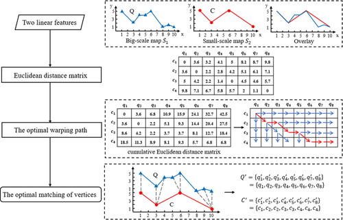
Figure 1 illustrates the flow chart of matching two linear features with the different number of vertices by DTW algorithm. Suppose that $Q:\{q_1,q_2,q_3,q_4,q_5,q_6,q_7,q_8\}$ and $C:\{c_1,c_2,c_3,c_4\}$ are two representations of the same linear feature at a large scale $S_1$ and small scale $S_2,$ polyline Q has 8 vertices and polyline C has 4 vertices. Firstly, the Euclidean distance of each pair of vertices is calculated. Then, all possible paths from the upper-left corner to the bottom-right one are enumerated by DP algorithm, and the optimal warping path (red curve) can be identified by tracking back along the arrows based on the cumulative Euclidean distance matrix. Finally, according to the trend of the optimal warping path, we can obtain the optimal matching relationship between the points in two coordinate sequences, that is, $c_1$ corresponds to $q_1,$ $c_2$ corresponds to $q_2$ and $q_3,$ $c_3$ corresponds to $q_4$ and $q_5,$ $c_4$ corresponds to $q_6, q_7$ and $q_8.$ In order to align the points of set Q and C, a point identical to $c_2$ is added into set C at the same position of $c_2,$ then the original point $c_2$ can be corresponded to $q_2,$ and the newly added point can be corresponded to $q_3.$ Similarly, two points identical to $c_4$ are added into set C at the same position of $c_4,$ then the original point $c_4$ can be corresponded to $q_6,$ and the two newly added identical points can be corresponded to $q_7$ and $q_8.$ After the alignment, the polyline Q and C can be written as $Q\prime :\{q_1,q_2,q_3,q_4,q_5,q_6,q_7,q_8\},$ $C\prime :\{c_1,c_2,c_2,c_3,c_3,c_4,c_4,c_4\}.$

Figure 1. Flow chart of matching two linear features in different scales by DTW algorithm.

3.3. Continuous generalization based on morphing

After matching the vertices of two linear features, the aligned sequence $Q^{\prime }:\{q_1^{\prime },q_2^{\prime },\dots ,q_k^{\prime },\dots ,q_K^{\prime }\}$ in big-scale map $S_1$ and $C^{\prime }:\{c_1^{\prime },c_2^{\prime },\dots ,c_k^{\prime },\dots ,c_K^{\prime }\}$ in small-scale map $S_2$ have an equal number of vertices, where $q_k^{\prime }=\left(x_k^q,y_k^q\right), c_k^{\prime }=\left(x_k^c,y_k^c\right), k\in K.$ Assuming that $L_{RS}$ is the intermediate representation in the middle scale map $RS,$ where $L_{RS}={\{l}_1,l_2,\dots ,l_k,\dots ,l_K\},l_k=(x_k^l,y_k^l),k\in K.$ According to the morphing model in formula (1) and formula (2), the coordinate of each vertex in $L_{RS}$ can be calculated as: (6) $$\begin{array}{c}{l}_k=\left(1-T\right){\mathrm{*}q}_k^{\prime }+T*c_k^{\prime }\end{array}$$(6)

Where $T$ is a normalized weight parameter about intermediate-scale $RS,$ the greater the value of T means the closer the coordinate is to $c_k^{\prime },$ and the smaller the value of T means the closer the coordinate is to $q_k^{\prime }.$ A linear geographical feature is composed of multiple vertices, after calculating the coordinates of all vertices in the line $L_{RS},$ we can get the intermediate shape of continuous generalization based on the morphing method.

4. Experiment and discussion

4.1. Morphing experiment and analysis on simulated data

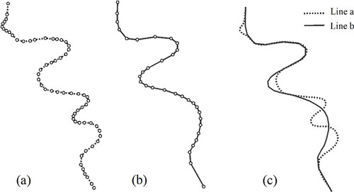
The map generalization operators used for scale transformation of linear features include vertex deletion, bend deletion, bend exaggeration and bend typification. The vertex deletion can be considered as the deletion of small bends. We use the simulation data in Figure 2 to analyze the feasibility of the DTW distance-based morphing method in the following three scenarios: bends typification, bends exaggeration and bends (vertices) deletion. Figure 2a is a finer representation of 62 vertices with rich details at a large scale, which is recorded as ‘line a’. Figure 2b is the related coarse representation of 33 vertices with fewer details at a small scale, which is generalized from line a and recorded as ‘line b’. Figure 2c is the overlapping representation of line a and line b, from which we can see the typical generalization operations of bend typification, bend exaggeration and bend deletion.

Figure 2. The simulated data with different levels of detail. (a) Large-scale representation. (b) Small-scale representation. (c) Overlapping representation.

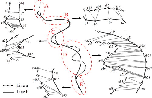
Figure 3 illustrates the details of simulation data in the scale transformation and the corresponding relationship of vertices between line a and line b. Area A is generated by bend deletion, area B and area E are generated by vertex deletion, area C is generated by bend exaggeration, and area D is generated by bend typification that reduces two bends to one bend. The coordinated sequence of line a and line b can be written as $a=\left\{a_1, a_2,\dots ,a_{62}\right\}$ and $b=\left\{b_1, b_2,\dots ,b_{33}\right\}.$ After alignment by DTW algorithm, the number of vertices of line a and line b can be equal, which has 78 vertices.

Figure 3. The corresponding relationship of vertices between line a and line b.

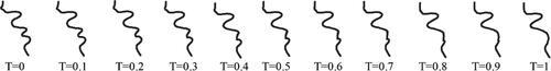
Figure 4 shows the continuous generalization effect of the simulated data based on the DTW distance-based morphing method. The shapes of T = 0 and T = 1 are the representation of linear features at the large scale $S_1$ and the small scale $S_2$ respectively, and the shapes from T = 0.1 to T = 0.9 are the results of shape interpolation, the relation between value T and the intermediate scale $Rs$ is shown in formula (2). From Figure 4 we can see that with the continuous increase of T, the curve shape of intermediate scale $Rs$ is more and more similar to that of small scale $S_2,$ and the bend typification, bend exaggeration and bend deletion operations have a smooth transition from left to right.

Figure 4. The morphing effect of DTW distance-based morphing method.

Additionally, we calculate the DTW distance as the shape similarity distance between the intermediate-scale shape (T = 0.1 to T = 0.9) and the large-scale (T = 0), and between the intermediate-scale shape (T = 0.1 to T = 0.9) and the small-scale shape (T = 1). The smaller the DTW distance means the higher the similarity between the two shapes. As shown in Table 1, the shape similarity distance between the large-scale shape and the small-scale shape is 0.16, a large value of T corresponds to a low similarity between intermediate-scale shapes and the large-scale shape $S_1,$ and a high similarity between intermediate-scale shapes and the small-scale shape ${ S}_2,$ which is consistent with the previous study (Li et al. 2017b).

Table 1. Similarity distance of shapes between intermediate scales and initial scales by the proposed method for simulated data.

T	0	0.1	0.2	0.3	0.4	0.5	0.6	0.7	0.8	0.9	1
$S_1$	0	0.027	0.050	0.071	0.091	0.11	0.13	0.15	0.17	0.19	0.16
${ S}_2$	0.16	0.21	0.19	0.17	0.14	0.12	0.10	0.081	0.054	0.027	0

4.2. Comparative experiments and analysis

In order to analyze the effect of the method proposed in this paper, we conduct comparative experiments using linear interpolation (Nöllenburg et al. 2008) and Fourier transformation-based morphing method (Li et al. 2018) for the data in Section 4.1. For the linear interpolation method, we first build a one-to-one correspondence between two curves at the vertex level. Then the linear interpolation is performed between the corresponding coordinate points to get the shapes at intermediate scales. For Fourier transformation-based morphing method, we first convert the two curves into two Fourier series. Then combine the two Fourier series to get the intermediate function, based on which the shapes in vector at intermediate scales can be restructured by inverse Fourier transform.

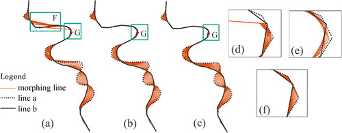
The comparison results are shown in Figure 5, in which Figure 5a–c are the morphing results by the linear interpolation method, Fourier transformation-based morphing method, and the proposed DTW distance-based method respectively, Figure 5d–f are the effects of partially zooming in on region G respectively. From Figure 5a we can see that the morphing results by linear interpolation method have some obvious morphological distortion at intermediate scales, especially in region F. From Figure 5e and f we can see that the proposed morphing method can maintain the original characters of two linear features (see Figure 5f), but the Fourier based-method replaces the gradient of a polyline with a smooth gradient, which also distorts the original geometric characteristics of the curves to a certain degree (see Figure 5e). Through the comparative experiments, we can conclude that the morphing method proposed in this paper is more suitable for the scale transformation of linear features in maps.

Figure 5. Overlaps of the morphing results through the (a). linear interpolation method; (b). Fourier transformation-based morphing method and (c). proposed DTW distance-based morphing method; (d)-(f). close-up of region G.

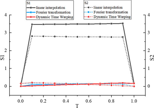
Furthermore, we use the DTW algorithm to calculate the similarity distance between the intermediate shapes and the initial shapes as a quantitative evaluation of the morphing effect. The smaller the DTW distance means the higher the similarity between the two shapes, the better the matching effect and the better the morphing transformation effect. As shown in Figure 6, we found that most of the black and blue nodes are above the red nodes, which means the shape similarity distance obtained by the linear interpolation method or Fourier transformation-based method is higher than that based on the proposed method, indicating that the proposed DTW distance-based method can effectively improve the accuracy of matching and morphing.

Figure 6. Similarity distance of shapes between intermediate scales and initial scales by linear interpolation method, Fourier transformation-based morphing method, and DTW distance-based morphing method.

4.3. Applications of DTW distance-based morphing for continuous generalization

In this section, the DTW distance-based morphing method is tested for continuous generalization of real linear geographical features. Two groups of typical linear geographical features, river and contour line, are used in the experiment. The data is sourced from the National Fundamental Geographic Information System of China, including 21 rivers and 30 contour lines. Each group of datasets consists of an original shape at the large scale $S_1$ and a target shape at the small scale $S_2.$ The scale of the source shape is 1:10000 (Figures 7a and 8a), and the scale of the target shape is 1:50000 (Figures 7f and 8f). The sequence of the intermediate scale is 1:18000, 1:26000, 1:34000, 1:42000, and the corresponding values of T are 0.2, 0.4, 0.6, 0.8, which are shown in Figures 7b–e and 8b–e.

Figure 7. Continuous generalization of river networks by DTW distance-based morphing method.

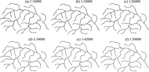
Figure 8. Continuous generalization of contour lines by DTW distance-based morphing method.

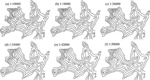
From Figures 7 and 8 we can see that, for the river networks, the results of continuous generalization preserve the connectivity and the network structures of linear geographical features; for the contour lines, the morphological characteristics of valleys and ridges are retained without topological errors. Therefore, the DTW distance-based morphing method can maintain the geometric and topological structure of linear features during the process of continuous scale transformation.

Table 2 is the shape similarity distance of the real linear features (river and contour) between the intermediate scale (T = 0.1 to T = 0.9) and the large-scale shapes (T = 0), and between the intermediate scale (T = 0.1 to T = 0.9) and the small-scale shapes (T = 1), which is obtained by summarizing the DTW distance of all lines in river and contour. It can be seen that for the real river, the shape similarity distance between large-scale shape and small-scale shape is 116.332, and for the contour line, the distance is 9.861. Similar to the result of the simulated data, the value T is significantly correlated with the scale, a large value of T or $Rs$ corresponds to a low similarity between middle shapes and the large-scale shape and a high similarity between middle shapes and the small-scale shape.

Table 2. Similarity distance of shapes between intermediate scales and initial scales for rivers and contours.

T		0	0.2	0.4	0.6	0.8	1
1/$Rs$		10000	18000	26000	34000	42000	50000
Rivers	$S_1$	0	29.038	55.659	82.106	107.962	116.332
	${ S}_2$	116.332	109.179	83.854	59.481	34.58	0
Contours	$S_1$	0	2.725	4.723	6.859	9.191	9.861
	${ S}_2$	9.861	8.982	6.746	4.497	2.355	0

5. Conclusions

We propose a morphing method for continuous generalization of linear features based on DTW distance in this study. In this method, we first establish an optimal matching of all vertices between two shapes in two different scales, and then employ the linear interpolation method to dynamically generate geometric shapes on any intermediate scale. The geometrical feature of the same entity at different scales often has a different number of vertices, thus there exists a one-to-many corresponding relationship between two shape vertices. Vertex matching plays an important role in shape morphing, unreasonable matching may directly lead to poor morphing results. In this paper, we use the DTW algorithm to find the optimal matching relationship of all vertices between two lines, which considers the global structure of features by calculating the overall similarity between linear features at different scales through the DTW distance. Meanwhile, it can directly obtain the optimal alignment relationship of all vertices, which is simple and operable. The case study shows that the DTW distance-based morphing method is suitable for the continuous generalization of linear features. In the practical application of real linear features, the geometric characteristics and the topological structure are well preserved.

It should be noted that if the change of the map scale is too big, the geometric dimensions of map objects may change. For example, on a 1:10000 map, a river feature is represented as a polygon, but on a 1:100000 map, it may be represented as a polyline. The morphing method is only applicable for the map objects with the same geometric dimension, it cannot realize the transformation from polyline to polygon, or from point to polyline.

CRediT authorship contribution statement

Jingzhong Li: Develop the proposed approach, guide the conducted research in general and write the paper. Kainan Mao: Evaluate the proposed algorithm, develop the code and write the paper.

Code availability

The python code for the DTW algorithm to measure the similarity distance of linear features is available at the link: https://github.com/mao2023/mao_paper

Disclosure statement

No potential conflict of interest was reported by the authors.

Additional information

Funding

This work was supported by the Open Fund of Key Laboratory of Urban Land Resources Monitoring and Simulation, Ministry of Natural Resources [Grant number KF-2022-07-017]; the National Natural Science Foundation of China [Grant number 42271454]; the Open Research Fund of Key Laboratory of Digital Earth Science [Grant number 2022LDE004]; the LIESMARS Special Research Funding.

References

- Belgiu M, Zhou Y, Marshall M, Stein A. 2020. Dynamic time warping for crops mapping. Int Arch Photogramm Remote Sens Spatial Inf Sci. 43:947–951.
- Berndt DJ, Clifford J. 1994. Using dynamic time warping to find patterns in time series. In: Proceedings of the 3rd International Conference on Knowledge Discovery and Data Mining. Seattle, WA: AAAI Press; p. 359–370.
- Cecconi A, Galanda M. 2002. Adaptive zooming in web cartography. In: Computer Graphics Forum. Vol. 21; p. 787–799.
- Cecconi A. 2003. Integration of cartographic generalization and multi-scale databases for enhanced web mapping [doctoral dissertation]. Switzerland: ETH Zurich.
- Csillik O, Belgiu M, Asner GP, Kelly M. 2019. Object-based time-constrained dynamic time warping classification of crops using sentinel-2. Remote Sensing. 11(10):1257. Available from: https://www.mdpi.com/2072-4292/11/10/1257.
- Danciger J, Devadoss SL, Mugno J, Sheehy D, Ward R. 2009. Shape deformation in continuous map generalization. Geoinformatica. 13(2):203–221.
- Deng M, Peng D. 2015. Morphing linear features based on their entire structures. Trans GIS. 19(5):653–677. Available from: https://onlinelibrary.wiley.com/doi/abs/10.1111/tgis.12111.
- Du J, Wu F, Xing R, Gong X, Yu L. 2022. Segmentation and sampling method for complex polyline generalization based on a generative adversarial network. Geocarto Int. 37(14):4158–4180.
- Fan W. 2014. Matching and classification model for multi-scale transformation and representation of spatial data. J Geomatics Sci Technol. 31(4):331–335.
- Gao A, Li J, Chen K. 2020. A morphing approach for continuous generalization of linear map features. PLoS ONE. 15(12):e0243328.
- Guan X, Liu G, Huang C, Meng X, Liu Q, Wu C, Ablat X, Chen Z, Wang Q. 2018. An open-boundary locally weighted dynamic time warping method for cropland mapping. ISPRS Int J Geo-Inf. 7(2):75. Available from: https://www.mdpi.com/2220-9964/7/2/75.
- Han L, Gao C, Zhang S, Li D, Sun Z, Yang G, Li J, Zhang C, Shao G. 2019. Speech recognition algorithm of substation inspection robot based on improved DTW. In: Advances in Intelligent, Interactive Systems and Applications: Proceedings of the 3rd International Conference on Intelligent, Interactive Systems and Applications (IISA2018) 3. Springer; p. 47–54.
- Izakian H, Pedrycz W, Jamal I. 2015. Fuzzy clustering of time series data using dynamic time warping distance. Eng Appl Artif Intell. 39:235–244. Available from: https://www.sciencedirect.com/science/article/pii/S0952197614003078.
- Jiang Y, Qi Y, Wang W, Bent B, Avram R, Olgin J, Dunn J. 2020. EventDTW: An improved dynamic time warping algorithm for aligning biomedical signals of nonuniform sampling frequencies. Sensors. 20(9):2700.
- Kaya H, Gündüz-Öğüdücü Ş., Ş., 2015. A distance based time series classification framework. Inf Syst. 51:27–42.
- Li J, Ai T, Liu P, Yang M. 2017a. Continuous scale transformations of linear features using simulated annealing-based morphing. ISPRS Int J Geo-Inf. 6(8):242.
- Li J, Fang W. 2018. Morphing polylines by preserving local neighborhood structures. Geomatics Inf Sci Wuhan Univ. 43(08):1138–1143.
- Li J, Li X, Xie T. 2017b. Morphing of building footprints using a turning angle function. ISPRS Int J Geo-Inf. 6(6):173.
- Li J, Liu P, Yu W, Cheng X. 2018. The morphing of geographical features by Fourier transformation. PLoS ONE. 13(1):e0191136.
- Li Z, Zhou Q. 2012. Integration of linear and areal hierarchies for continuous multi-scale representation of road networks. Int J Geogr Inf Sci. 26(5):855–880.
- Liu L, Wang G, Zhang B, Guo B, Shum H-Y. 2004. Perceptually based approach for planar shape morphing. In: 12th Pacific Conference on Computer Graphics and Applications, 2004. PG 2004. Proceedings.
- Liu P, Li X, Liu W, Ai T. 2016. Fourier-based multi-scale representation and progressive transmission of cartographic curves on the internet. Cartogr Geogr Inf Sci. 43(5):454–468.
- Liu P, Xiao T, Xiao J, Ai T. 2020. A multi-scale representation model of polyline based on head/tail breaks. Int J Geogr Inf Sci. 34(11):2275–2295.
- Lonergan M, Jones C. 2001. An iterative displacement method for conflict resolution in map generalization. Algorithmica. 30(2):287–301.
- Matsuoka A, Yoshioka F, Ozawa S, Takebe J. 2019. Development of three-dimensional facial expression models using morphing methods for fabricating facial prostheses. J Prosthodontic Res. 63(1):66–72. Available from: https://www.sciencedirect.com/science/article/pii/S1883195818302287.
- Nöllenburg M, Merrick D, Wolff A, Benkert M. 2008. Morphing polylines: A step towards continuous generalization. Comput Environ Urban Syst. 32(4):248–260.
- Pantazis D, Karathanasis B, Kassoli M, Koukofikis A, Stratakis P. 2009b. Morphing techniques: towards new methods for raster based cartographic generalization. In: Proceedings of the 24th International Cartographic Conference.
- Pantazis DN, Karathanasis B, Kassoli M, Koukofikis A. 2009a. Are the morphing techniques useful for cartographic generalization? In: Alenka Krek, Massimo Rumor, Sisi Zlatanova, Elfriede M. Fendel, editors. Urban and regional data management. London: CRC Press; p. 207–216.
- Peng D, Wolff A, Haunert J-H. 2016. Continuous generalization of administrative boundaries based on compatible triangulations. In: Geospatial Data in a Changing World: Selected Papers of the 19th Agile Conference on Geographic Information Science.
- Permanasari Y, Harahap EH, Ali EP. 2019. Speech recognition using dynamic time warping. In: Journal of physics: Conference Series. Vol. 1366. IOP Publishing; p. 012091.
- Sederberg T, Gao P, Wang G, Mu H. 1993. 2-D shape blending: An intrinsic solution to the vertex path problem. In: Proceedings of the 20th Annual Conference on Computer Graphics and Interactive Techniques.
- Sederberg T, Greenwood E. 1992. A physically based approach to 2-d shape blending. In: Proceedings of the 19th Annual Conference on Computer Graphics and Interactive Techniques. Vol. 26; p. 25–34.
- Shen Y, Ai T, Li J, Huang L, Li W. 2020. A progressive method for the collapse of river representation considering geographical characteristics. Int J Digital Earth. 13(12):1366–1390.
- Steyvers M. 1999. Morphing techniques for manipulating face images. Behav Res Methods Instrum Comput. 31(2):359–369.
- Stoter J, Burghardt D, Duchêne C, Baella B, Bakker N, Blok C, Pla M, Regnauld N, Touya G, Schmid S. 2009. Methodology for evaluating automated map generalization in commercial software. Comput Environ Urban Syst. 33(5):311–324. Available from: https://www.sciencedirect.com/science/article/pii/S0198971509000465.
- Šuba R, Meijers M, Oosterom P. 2016. Continuous road network generalization throughout all scales. Int J Geo-Inf. 5(8):145.
- Surazhsky V, Gotsman C. 2003. Intrinsic morphing of compatible triangulations. Int J Shape Model. 09(02):191–201.
- Van Kreveld M. 2001. Smooth generalization for continuous zooming. In: Proceedings of the 20th International Geographic Conference; p. 2180–2185.
- Whited B, Rossignac J. 2009. B-morphs between b-compatible curves in the plane. In: 2009 SIAM/ACM Joint Conference on Geometric and Physical Modeling
- Wilson ID, Ware JM, Ware JA. 2003. A genetic algorithm approach to cartographic map generalisation. Comput Ind. 52(3):291–304. Available from: https://www.sciencedirect.com/science/article/pii/S0166361503001325.
- Yamazaki S. 2007. Warping and morphing. In: Benjamin W. Wah, editor. Wiley encyclopedia of computer science and engineering. Wiley Online Library.
- Yang B, Purves R, Weibel R. 2007. Efficient transmission of vector data over the internet. Int J Geogr Inf Sci. 21(2):215–237.
- Yang W, Feng J. 2009. 2d shape morphing via automatic feature matching and hierarchical interpolation. Comput Graphics. 33(3):414–423. Available from: https://www.sciencedirect.com/science/article/pii/S0097849309000387.
- Yuefeng Z. 1996. A fuzzy approach to digital image warping. IEEE Comput Graphics Appl. 16(4):34–41.
- Zhu L, Zhong S, Tu W, Zheng J, He S, Bao J, Huang C. 2019. Assessing spatial accessibility to medical resources at the community level in shenzhen, china. Int J Environ Res Public Health. 16(2):242.