Vegetation structural composition mapping of a complex landscape using forest cover density transformation and random decision forest classifier: a comparison

Abstract

Forest cover density (FCD) transformation and random decision forest (RDF) classification have been widely used for vegetation mapping. Nevertheless, a comparison of their capabilities in complex tropical landscapes is still rarely carried out. This study compared the two methods using Landsat-8 OLI imagery which includes the blue up to thermal bands for vegetation structural composition mapping in a complex landscape of Central Java, Indonesia. We used the FCD transformation with six indices to generate 11 classes, while the RDF classified the same 11 classes based on training areas and used a random process involving various number of splits and trees. The results showed that the FCD transformation achieved 69.32% accuracy, while the RDF was able to classify the 11 classes with various accuracies depending on the parameter setting, i.e. from 70.76% to 75.19%. Regarding the obtained accuracies, problems associated with the terrain and vegetation characteristics have been discussed for further recommendation.

Keywords:

• Vegetation structural composition
• complex landscape
• forest cover density
• random decision forest

1. Introduction

1.1. Background

Vegetation mapping is an important part of the land resource inventory. This activity has been done at various levels, from local to global scopes (Küchler and Zonneveld 1988; Franklin 2013). Analysis of the vegetation area shrinkage is not only based on the extent of coverage but also on the quality. The quality of vegetation coverage can be seen from its structural composition and diversity. Remote sensing as a science provides a wide range of methods for land-cover/land-use studies, including vegetation density estimates and classification (Giri 2012; Zaehringer et al. 2018). In digital image analysis, vegetation study and mapping usually make use of vegetation index based as well as multispectral classification approaches. The vegetation index-based approach can highlight the density but is generally unable to show heterogeneity if structural and floristic compositions are taken into consideration. On the other hand, the multispectral classification can distinguish categories including heterogeneity but it does not show the density quantitatively (Danoedoro 2019). In addition to mapping of natural vegetation areas, information extraction of vegetation density and structural composition also needs to be carried out in areas with mixed land-cover/land-use to analyse heterogeneity that is related to human intervention (Danoedoro and Gupita 2022).

Indonesia is located in a wet tropical region with very complex phenomena of landscapes. Several islands were predominantly formed by tectonic forces, while some others were strongly influenced by volcanic activities. In volcanic islands like Java, the elevation range is very wide, from 0 up to more than 3000 m above sea level (asl), which makes a great variation in temperature, humidity, and rainfall. The combination between parent materials, climate, and topography leads to the different developments of natural, semi-natural and cultivated vegetations (van Gils et al. 1990; Huggett and Cheesman 2002). Intensive encroachment of human population to the naturally vegetated areas during the past 100 years also causes a specific phenomenon showing interleave between various types of vegetation and man-made features. From an ecological perspective, this landscape arrangement is interesting to map using vegetation ecological approaches based on remotely sensed imagery. Remote sensing with vegetation ecological approach tries to identify and classify either structural or floristic composition of vegetation by considering terrain characteristics such as geology, landform, climate, soil, and hydrology (Küchler and Zonneveld 1988; van Gils et al. 1990; Ohno 1991). In practice, vegetation information is extracted using either visual or digital image analysis, while the terrain characteristics are interpreted visually, and the results are processed in a GIS environment (Danoedoro 2019).

Vegetation index transformation is usually applied for quantitative mapping of vegetation density levels (Xue and Su 2017), but this model is not intended to distinguish variations in structural composition. On the other hand, multispectral classification is often carried out to distinguish various types of vegetation including their structural composition as categorical classes (Danoedoro et al. 2020). The Forest Cover Density (FCD) model was developed by ITTO (Rikimaru et al. 2002) to overcome the weaknesses of most vegetation indices, particularly the ratio- and normalized difference-based ones such as simple ratio and NDVI, and at the same time it is intended to present quantitative structural composition information (Bera et al. 2020). This model is also claimed to overcome the problem of inability to distinguish the vegetation index values indicated by high density grass (e.g. rice) from high density forest due to the saturation effect (Deka et al. 2019; Abdollahnejad et al. 2017; Hartoyo et al. 2019).

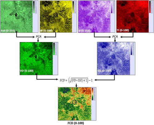
The FCD model is an empirical deductive-deterministic model. It is a rule-based approach and is usually applied to natural/semi-natural vegetation coverage using six input bands of Landsat series, i.e. blue, green, red, near infrared, first middle infrared (SWIR1) and thermal infrared (Rikimaru et al. 2002). The FCD transformation combines six kinds of indices called the advanced vegetation index (AVI), bare soil index (BI), shadow index (SI), thermal index (TI), vegetation density (VD), and shadow scaled index (SSI). VD is derived from the integration of AVI and BI, while SSI is derived from a combination of SI and TI. The combination of VD and SSI produces FCD images with a value range of 0–100 which shows the density level from open land (0% vegetation coverage) to very heterogeneous forest vegetation with a canopy density of 100%, and at the same time can be classified into structural composition classes into 11 classes. It should also be noted that the FCD model was developed to minimize fieldwork. The FCD-based mapping activities were also sometimes carried out without fieldwork (ITTO 1997)

Ho (1995) stated that Random Decision Forest (RDF) is a method to build multiple trees in randomly selected subspaces of the feature space. Eastman (2019) stated that Random Decision Forest (RDF) or simply called Random Forests (RF), a machine learning algorithm developed by Breiman (2001) and then Breiman and Cutler (2005), which tries to overcome the weakness of decision trees. The RDF, according to Eastman (2019), uses training data and a set of explanatory variables, such as remotely sensed reflectance bands, and it produces a hard classification as well as an optional set of soft probability images. The RDF or RF has also been used in remote sensing classification analysis. In the process, RF uses a strategy of a random sample selection process and bootstrap aggregating (bagging) with a resample process (with a replacement sample) to create a new decision tree (Biau 2012). The RF algorithm applies a bagging process to evaluate the model based on samples that are not used in the decision tree, and produces out-of-bag error values (OOB). In addition, the randomization process at the time of tree creation makes the RF less susceptible to overfitting which in this case makes the model more accurate in modelling the training data. This randomization process has also been widely developed because it can improve the accuracy of RF modelling (Smith et al. 2013; Fawagreh et al. 2014).

RF algorithms have been widely applied to remote sensing studies, including for classification tasks such as rice field classification/identification, and prediction of vegetation biophysical information (Arjasakusuma et al. 2020, 2021). This algorithm can also be accessed using cloud computing platforms, such as Google Earth Engine (GEE) (Gorelick et al. 2017), which is useful for processing large volumes of remotely sensed data.

With respect to the described background, a relatively conventional vegetation mapping method using forest cover density (FCD) transformation should be compared with more recent machine learning-based classification methods, by using complex terrain characteristics and complex vegetation structural composition as a testing area. This study needs to be carried out to have a better understanding of the vegetation structural composition mapping based on recently developed classification methods like machine leaning-based random forest, which has been claimed as an accurate method for many land-cover classification purposes. On the other hand, several studies showed that the FCD transformation methods produced inconsistent results with various levels of accuracy (Himayah et al. 2016; Abdollahnejad et al. 2017; Danoedoro and Gupita, 2022).

1.2. Study objective

Based on the described background and problem statement, this study aimed to compare the performance of rule-based FCD transformation and machine learning-based RDF classification for mapping the vegetation structural composition in Salatiga – Ambarawa and its surrounding, Central Java, which exhibits a wet tropical complex landscape of Indonesia.

Many studies related to vegetation structural composition mapping using FCD transformation (e.g. Himayah et al. 2016; Deka et al. 2019; Salsabila and Danoedoro 2021) and RDF/RF classifier (e.g. Fu et al. 2017; Mohammadpour et al. 2022) did not pay particular attention on the complexity of landscape characteristics with respect to the obtained accuracies. Therefore, this study sought to provide a better understanding of the advantages and limitations of both methods in vegetation structural composition mapping in complex tropical landscapes such as in Indonesia. In addition, even though the FCD transformation has been widely used, results presented in literature are inconsistent in terms of their accuracy, especially when they are derived using different algorithms in different softwares (Himayah et al. 2016; Salsabila and Danoedoro 2021; Danoedoro et al. 2022). Therefore, a machine learning approach needs to be tried to see whether a model based on spectral transformation with a series of indices can be replaced by RDF classification.

2. Materials and methods

2.1. Study area

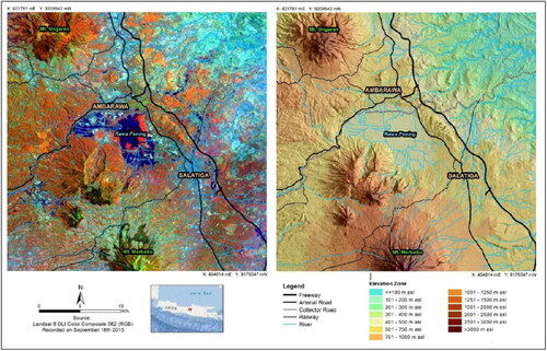
The landscape of the Salatiga-Ambarawa area, Central Java, represents a combination between volcanoes, structural hills, and lacustrine plains of wet tropical region, which are covered by various types of vegetation and occupied for various categories of land-use (van Bemmelen 1949; Pratama and Danoedoro 2020; Danoedoro et al. 2022). This area covers Merbabu volcano with an elevation of 3142 m above sea level (asl) in the south, and Ungaran volcano in the north-west (2050 m asl). In the north-eastern part, there is a low hilly terrain with an altitude range from 100 to 250 m asl, while in the middle is a fluvial basin with eutrophicating lake of Rawa Pening, a lacustrine plain at an altitude of around 470 m asl (Piranti et al. 2019). The town of Salatiga is a part of the foot slopes of Merbabu volcano at an altitude of about 550–700 m asl, while Ambarawa is another small town in the foot slope of Ungaran volcano (2000 m asl). Figure 1 summarizes this description.

Figure 1. Study area as presented using Landsat false colour composite and SRTM hillshade images.

The mixture of vegetation, water, building, and barren land shows very complex land-cover as viewed from its structural compositions. Various types of vegetation, from very high-density montane forest, medium density forest, industrial plantation forest, shrubs, mixed trees, plantation with perennial crops (rubber, coffee and cocoa), annual agricultural crops, and aquatic weed called enceng gondok (Eichhornia crasssipes) can be found in a mixture, although some categories only exist in particular environment. Trees as homestead gardens and mixed gardens appear alternately with settlements, thus presenting a variety of complex structural compositions, which cannot be found in most natural or semi-natural vegetation covers (Hadi and Danoedoro 2021). Therefore, vegetation structural composition mapping activities would face different problems as compared to its application in the majority forested land.

2.2. Data and materials

This study made use of Landsat 8 OLI covering the Salatiga – Ambarawa area and its surrounding, Central Java, at Path/Row 120/065, recorded in September 18^th 2018, which has been corrected geometrically at T level, as shown in Figure 1. The dataset consists of six bands ranging from blue (0.450–0.515 μm), green (0.525–0.600 μm), red (0.630–0.680 μm), near infrared (NIR) (0.845–0.885 μm), and short-wave infrared-1 (SWIR1) (1.550–1.660 μm), which were recorded at 30 m spatial resolution, as well as thermal infrared (band 10) (10.30–11.30 μm) that has been resampled from 100 m to 30 m pixel size, as developed and explained by Rikimaru et al. (2002), which said that the use of thermal band differentiate multistorey forest canopy from high density grassland, where the forest canopy tends to be cooler. This study also utilized WorldView imagery covering some parts of the study area (particularly the city of Salatiga and its surrounding) and RBI topographic map at 1:25,000 scale as a basis for field orientation, measurement, and field reference during accuracy assessment. We used ILWIS Open for image processing and spatial analysis software, particularly to process the FCD transformation, and Idrisi/Terrset image processing/GIS software for radiometric correction and classification using machine learning, particularly with random decision forest (RDF) algorithm.

2.3. Methods

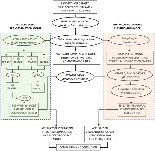
This study consists of two main methods, namely FCD transformation and machine learning-based classification with RDF. To compare the two, we used the Landsat 8 OLI dataset with the same spectral bands, i.e. blue, green, red, NIR, SWIR1 and thermal infrared of band 10. The dataset al.so geometrically and radiometrically corrected. For radiometric correction, Chavez’s full model correction method (Chavez 1996; Eastman 2019) applied. Figure 2 shows a flow chart in this research method. The FCD-generated vegetation structural composition map was then compared with the best result obtained using RDF classification. Prior to the comparison, we evaluated the RDF classification by using the out of bag (OOB) accuracy, overall accuracy, and Kappa index of each derived map as a result of a particular combination between number of the split variable (i.e. input spectral bands) and the number of decision trees. Field reference for accuracy assessment of both FCD transformation and RDF classification results was developed using a collection of independent datasets in the forms of polygons.

Figure 2. Methods flowchart.

2.3.1. Radiometric correction

The original Landsat-8 OLI image was available in 16-bit coding format or has a range of digital number (DN) 0–65,535. Since the FCD model was developed based on 8-bit coding Landsat-5 TM and Landsat-7 ETM + images, the correction used full atmospheric correction to derive new dataset with 0–1.0 range of at surface reflectance. This new dataset was then stretched to 0–255 DN range. The equation of full atmospheric correction was based on the work of Chavez (1996) as follows: (1) $$\rho =\frac{\left(\Pi \mathrm{*}\right(L_{\lambda }-L_{\mathit{haze}}\left)\right)}{\left({\tau }_v\mathrm{*}\right(E_o\mathrm{*}\mathrm{Cos}\left(T_Z\right)\mathrm{*}{\tau }_z+E_{\mathit{down}})}$$(1) where ρ is at-surface reflectance in percent, L_λ is the image spectral radiance, L_haze is scattered spectral radiance recorded as the minimum one by the sensor, τ_v is the atmospheric transmittance or optical thickness of the atmosphere, E_o is the solar spectral irradiance, which takes into account the Earth-Sun distance in specific Julian day, T_z is the incident angle of the direct solar flux to the Earth surface, and E_down is downwelling spectral irradiance due to the scattered solar flux in the atmosphere.

2.3.2. FCD transformation

The FCD transformation generated vegetation density and structural composition map with a value range of 0–100 and was classified into 11 classes as presented in Table 1. This study modified the original FCD class description to accommodate the presence of water and buildings in the study area.

Table 1. Original classification of forest cover density (FCD) which is translated to new vegetation structural composition for this study.

Class	Value Range	FCD Vegetation structural composition description	Short description of vegetation structural composition for this study
0	0	Bare soil	Bare soil, building, or water body
1	1–10	No canopy coverage. Open land and grass are predominant	Very sparse bushy grassland or urban building with very sparse vegetation
2	11–20	Tree canopies began to emerge but open soil is still predominat,	Sparse wooded bushy grassland or urban/rural buildings with sparse vegetation
3	21–30	Tree canopies occupy 11–20% of the pixel area but open land is still predominant	Sparse wooded bushland or rural buildings
4	31–40	Tree canopies occupy 21–30% of the pixel area interleaved with bushes and shrubs	Denser wooded bushland
5	41–50	Young tree canopies develop and cover 41–50% of the pixel area, with a predominance of shrubs while shrubs decrease.	Woodland
6	51–60	Adult and young tree canopies are growing, covering 51–60% of the pixel area which is starting to show a difference	Woodland with multi-story trees
7	61–70	Tree canopies are growing rapidly covering 61–70% of the pixel area with differences in strata of stands, clearly visible and heterogeneous	Heterogeneous moderate density forest
8	71–80	Tree canopies cover 71–80% of the pixel area with distinct strata standing distinctions, species heterogeneity is increasing,	Heterogeneous dense forest
9	81–90	Tree canopies cover 81–90% of the pixel area with different standing strata; very clearly seen, very high heterogeneity	Heterogeneous very dense forest
10	91–100	Tree canopies cover 91–100% of the pixel area with very stratified differences, very high heterogeneity, sunlight is unable to reach the forest floor and moisture is very high.	Extremely dense forest

Modified from Rikimaru (2002).

To achieve this result, in the initial stage we transformed the six Landsat 8 OLI spectral bands to four indices, namely Advanced Vegetation Index (AVI), Soil Brightness Index (BI), Shadow Index (SI), and Thermal Index (TI). According to Rikimaru et al. (2002), the AVI and BI were then combined using principal component analysis (PCA), where the resultant PC1 becomes derived data called Vegetation Density (VD), while the SI and TI were also integrated with PCA to produce derived data in the form of Shadow Scale Index (SSI). The VD was inverted and rescaled with respect to the newly defined 0% and 100% of vegetation cover, respectively, while the SSI was linearly transformed with respect to new 0% (no shadow) and 100% (fully covered by forest). The final result is FCD value derived from combining VD and SSI images. Before applying all the formulas that make up the various indices and FCDs, all the original bands that have been corrected for at-surface reflectance were stretched to 0–255 range first (Danoedoro and Gupita 2022). This had to be done, because the original FCD formula developed by ITTO (Rikimaru et al. 2002) used an image with 8-bit coding.

The AVI involved the red (Red) and near infrared (NIR) bands. Since this formula contains NIR-Red terms, it is possible that the results obtained from NIR-Red <0, so that the following conditions were required:

IF (NIR-Red) ≤ 0,

THEN AVI = 0,

ELSE (2) $$\mathit{AVI}=\sqrt[3]{(\mathit{NIR}+1)\mathrm{*}(256-\mathit{Red})\mathrm{*}(\mathit{NIR}-\mathit{Red})}$$(2)

BI was obtained by involving the first shortwave infrared (SWIR1), near infrared (NIR), red (Red) and Blue (Blue) bands with the following formula: (3) $$BI=\left(\left(\frac{\left(\mathit{SWIR}1+\mathit{Red}\right)-\left(\mathit{NIR}+\mathit{Blue}\right)}{\mathit{WIR}1+\mathit{Red})+(\mathit{NIR}+\mathit{Blue})}\right)\mathrm{*}100\right)+100$$(3)

Where is 0 ≤ BI ≤ 200

These AVI and BI images were then integrated using PCA, where the first principal component (PC1) was taken as the VD or vegetation density image. These results were then transformed linearly into a new image with the 0–100 range, where 0 indicated bare soil (0% vegetation cover) and 100 indicated forest with 100% vegetation cover.

SI image was generated by involving blue, green and red bands, with the following formula: (4) $$SI=\mathrm{ }\sqrt[3]{\left(256-\mathit{Blue}\right)\mathrm{*}\left(256-\mathit{Green}\right)\mathrm{*}(256-\mathit{Red})}$$(4)

Thermal band of Landsat-8 OLI was used due to its capability to distinguish multistorey vegetation composition from very dense grass such as mature rice (Rikimaru et al. 2002). The thermal band was converted to spectral radiance image L_{λ_} through the following formula (Jensen 2015): (5) $$L_{\lambda \_\mathit{image}}=L_{\lambda \_\min }+\mathrm{ }\left(\frac{L_{\lambda \_\max }-L_{\lambda \_\min }}{{DN}_{\max }}\mathrm{*}{DN}_{\mathit{image}}\right)$$(5) where L_{λ_min} is the minimum detectable spectral radiance value in the corrected band, L_{λ_max} is the maximum detectable spectral radiance value, DN_max is the maximum DN of the original image (in 16-bit coding means 65,535), while DN_image denotes all image’s DNs to be calibrated to spectral radiance in Watt m⁻² sr⁻¹ µm⁻¹. The value L_λmin in this new image was then converted to 8-bit system (0–255) and was used as the thermal index image (TI) (Danoedoro and Gupita 2022).

In the next step, the SI and the TI images were then integrated with the PCA method to derive a new image called the Scaled Shadow Index (SSI). Areas with SSI value = 0 were regions with shadow value (SI) = 0 too. The area where SSI = 100 was the area with 100% shadow cover. This value range was then used as a basis for scaling back the SI value into a normalized SSI through a linear transformation process, where the original SI range was changed to 0–100, to represent the percentage of 0–100% vegetation cover.

Finally, the FCD map was derived from the VD and SSI images using the following formula: (6) $$\mathit{FCD}=\mathrm{ }\left(\sqrt{\left(VD\mathrm{*}\mathit{SSI}\right)+1}\right)-1$$(6) where it is assumed that FCD would have a range of 0–100, with 0 representing open land and 100 representing very dense vegetation with multiple layers (multistory). The generated FCD pixel values were then classified into 11 classes, as shown in Table 1.

2.3.3. Machine learning-based multispectral classification using RDF

The algorithm is briefly described as follows: First, it assumes that the training set has a size N, and the number of independent variables is equal to M. Then the algorithm adds three input parameters, i.e. a ratio r (0 ≤ r ≤ 1), a number of attributes m ≤ M, and a number of trees Ntree ≥ 1. By using primary training set, the algorithm generates a random sample without repetitions. The training set elements that failed to get into the sample be used later for estimating the generalization error. Based on the generated samples, the algorithm grows a decision tree. For each node of the tree, it randomly chooses m variables on which to base the decision at that node. Following this procedure, it then calculates the best split based on these m variables in the training set. The difference of RDF with the original RF algorithm, the tree is fully grown and is never pruned. The procedure is reiterated NTrees times. The trees grown unite to form a committee deciding by voting.

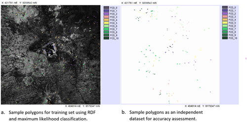
Unlike the FCD transformation, which is deterministic and deductive, RDF is a classification model that is inductive in character (because it uses spectral samples as training areas) and is based on stochastic processing. In this RDF, the authors used 241 polygon samples (12,049 pixels) representing the classes as presented in Table 1 and Figure 3, using high-resolution imagery and field observations. Figure 3 also shows a spatial distribution of independent dataset (142 polygons) which used as a field reference for the accuracy assessment of the FCD and RDF modelling results. The locations of samples were selected using a stratified random sampling strategy, and each sample consists of at least 50 times of the number of classes with respect to Costa et al. (2018). Referring to Table 1, each sample describes a certain category of structural composition that covers a certain canopy density class as well.

Figure 3. Distribution of training areas and independent data (in the form of polygons) for accuracy assessment.

The sampling strategy was carried out using stratified random sampling, where the strata were used are tentative spectral classes obtained using unsupervised classification with ISODATA (Jensen, 2015). The input for this ISODATA is the number of classes, the minimum number of pixels in each class, the spectral distance between classes, the standard deviation of each class, and the number of iterations. The distribution of sample points according to this strategy was delivered automatically using the spatial sampling module available in Idrisi/Terrset al.l selected points were then taken as samples in the form of polygons or regions of interest (ROI).

Furthermore, the RDF model is simulated with various scenarios including the number of splits or Mtry, and the number of trees (Ntree). For the number of splits, values of 2, 3, 4, 5 and 6 are used, where the maximum value of split 6 is the maximum number of variables (in this case the number of input spectral bands), while the number of decision trees were set from 50 to 400 with 50 increments. The Ntree of 50 was selected based on the previous studies stating that smaller number of trees will lead to less reliable probability estimates, while the large number of Ntree, i.e. more than 500, will lead to a slower classification stage (Eastman 2019).

In each simulation that consists of a unique combination between Mtry and Ntree, the OOB accuracy value was obtained as one of the bases for evaluating the results. However, accuracy assessment and comparison between FCD and RDF transformation-based models were undertaken by referring to independent field samples in the form of polygons. The accuracy value was determined by using the confusion matrix, which takes into account the producer’s and user’s accuracies in addition to the overall accuracy and Kappa index (Congalton and Green 2019). In addition, this study also compared the results (as a vegetation structural composition map) with the conventional multispectral classification result using the maximum likelihood algorithm.

3. Results and discussion

3.1. Radiometric correction and calibration

The dataset containing reflective bands was radiometrically corrected using equation (1)(1) $$\rho =\frac{\left(\Pi \mathrm{*}\right(L_{\lambda }-L_{\mathit{haze}}\left)\right)}{\left({\tau }_v\mathrm{*}\right(E_o\mathrm{*}\mathrm{Cos}\left(T_Z\right)\mathrm{*}{\tau }_z+E_{\mathit{down}})}$$(1) and derived at-surface reflectance images with pixel values at 0–1.0 range, where the 0 indicates very low reflectance, while the 1 shows the highest one. During the process, several pixels in each band also have values more than 1.0 but they have been neglected since the number of those pixels are less than 0.001% of the total pixels. These values were then set to 1.0, based on the assumption that they represent anomalous pixels. 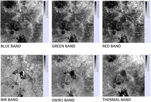The thermal bands were calibrated to spectral radiance using equation (5)(5) $$L_{\lambda \_\mathit{image}}=L_{\lambda \_\min }+\mathrm{ }\left(\frac{L_{\lambda \_\max }-L_{\lambda \_\min }}{{DN}_{\max }}\mathrm{*}{DN}_{\mathit{image}}\right)$$(5) and then rescaled to 0–100 for FCD modelling input and 0–1.0 for RDF classification input. Figure 4 shows the corrected and calibrated images.

Figure 4. Dataset containing blue, green, red, NIR, SWIR1 and Thermal bands that have been radiometrically corrected or calibrated.

3.2. Vegetation structural composition according to FCD model

Six indices have been derived from the dataset for constituting the FCD, as shown in Figure 4. Equation (2)(2) $$\mathit{AVI}=\sqrt[3]{(\mathit{NIR}+1)\mathrm{*}(256-\mathit{Red})\mathrm{*}(\mathit{NIR}-\mathit{Red})}$$(2) derived AVI image, and it shows the spectral variation where vegetation looks very bright while non-vegetated objects look dark. This appearance also shows that the AVI functions the same as other vegetation indices. However, the AVI model still shows a slight deviation, where high-density herbs such as aquatic weed of Eichhornia crassipes with water background are still of very high value, even higher than that of very dense forests. The same problem also found in the works of Salsabila and Danoedoro (2021), and Danoedoro and Gupita (2022). On the other hand, the BI model that generated using equation (3)(3) $$BI=\left(\left(\frac{\left(\mathit{SWIR}1+\mathit{Red}\right)-\left(\mathit{NIR}+\mathit{Blue}\right)}{\mathit{WIR}1+\mathit{Red})+(\mathit{NIR}+\mathit{Blue})}\right)\mathrm{*}100\right)+100$$(3) shows variations in brightness related to the presence of barren land as opposed to vegetation density, so that bare soil, building rooftops, water bodies, and impervious surfaces have very high values, in contrast to dense vegetation that shows very low one.

Equation (4)(4) $$SI=\mathrm{ }\sqrt[3]{\left(256-\mathit{Blue}\right)\mathrm{*}\left(256-\mathit{Green}\right)\mathrm{*}(256-\mathit{Red})}$$(4) produced SI model, which represents very high values in high density and heterogeneous forest due to shadow effect of the canopy, and very low values in barren land, building roof tops and other impervious surfaces. It is interesting to note, however, that SI also shows a slightly high value for water bodies, and this is shown in Lake Rawa Pening. On the contrary, the TI model produced by equation (5)(5) $$L_{\lambda \_\mathit{image}}=L_{\lambda \_\min }+\mathrm{ }\left(\frac{L_{\lambda \_\max }-L_{\lambda \_\min }}{{DN}_{\max }}\mathrm{*}{DN}_{\mathit{image}}\right)$$(5) provides the same information as temperature variations in the field, where barren land, impervious surfaces, and building rooftops tend to have very high values, while vegetation and water have very low ones. Apart from this appearance, the variation of terrain elevation in the study area also shows an interesting phenomenon, where the vegetation cover in very high elevations produces very low thermal index, even lower than that of water bodies. That is why Rikimaru et al. (2002) suggested that water and clouds should be masked first in order to overcome this problem.

Integration of AVI with BI to generate VD was carried out by implementing PCA. Since the two input indices are negatively correlated, the result of the transformation in the form of PC1 as the basis for developing VD actually shows a variation that is opposite to the vegetation index, where vegetation is negative, while open land is positive. Therefore, this PC1 image still requires further transformation in the form of inversion so that vegetation cover becomes bright and barren land becomes dark, ready to be rescaled to 0–100 by selecting pixels of barren land as 0 value and those of densest vegetation as 100. Integration using PCA also applied in combining SI and TI to derive the SSI image. The result of PC1 at this stage was also further processed to become SSI in a similar way as VD, where PC1 must be reversed first, then a new 0 value was determined based on pixels of barren land, while 100 value is determined using pixel values of very dense forest found in the field. In this case, no black soil or burnt soil were found, so the identification of black soil in the previous step according to Rikimaru et al. (2002) was not necessary.

Based on the rescaled VD and SSI inputs, the spatial distribution of density and the structural composition of vegetation in the study area could be determined using equation (6)(6) $$\mathit{FCD}=\mathrm{ }\left(\sqrt{\left(VD\mathrm{*}\mathit{SSI}\right)+1}\right)-1$$(6) . The result was a new image representing vegetation density and structural composition with a value range of 0–100. The values were then classified according to Table 1. Thus, the result of this modelling was a forest cover density map containing classes with nominal data (but at the same time can be viewed as ordinal data). Figure 5 shows the process and results.

Figure 5. Six indices used for generating FCD model. The result has a range of 0–100 that shows gradation of density as well as changes in structural composition.

Problems arose with the FCD modelling were not reported by several authors, e.g. Sukarna (2008), Ismail et al. (2017), Himayah et al. (2016), Hartoyo et al. (2019), and Ahmed (2020), who used semi-expert system software of FCD Mapper (ITTO/JOFCA 2003). This study used widely available softwares like ILWIS and Idrisi with map calculator and scripting capabilities for more flexible data conversion and analyses.

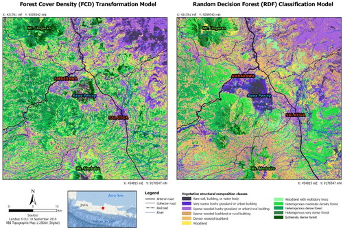
According to this original FCD transformation model, the landscape of Salatiga and its surroundings looks quite varied in terms of the vegetation structural composition, although the predominant classes are Class 3 (bushy grassland or urban/rural building, light-purple colour). In addition, classes of woodland, woodland with multistorey trees, and heterogeneous moderate density and heterogeneous dense forest also prominent (light – medium dark green). Figure 6 shows that classes of 10 and 11 (heterogeneous very dense forest and extremely dense forest) are mainly found in very steep and highly elevated mountainous areas. The distribution of each class with respect to the landform classes is presented in Table 2.

Figure 6. Vegetation structural composition model derived using FCD Transformation.

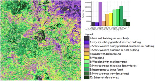
Table 2. Distribution of FCD classes according to the Landform units (in hectares), based on original FCD transformation.

	FCD0	FCD1	FCD2	FCD3	FCD4	FCD5	FCD6	FCD7	FCD8	FCD9	FCD10	TOTAL (ha)
Volcanic cone	65.13	9.3	108.6	46.86	136.02	174.75	301.56	372.72	462.66	250.74	202.08	2130.42
Volcanic upper slopes	13.68	3.72	432.42	168.66	392.73	497.07	770.97	903.21	1529.25	733.17	333.24	5778.12
Volcanic middle slopes	39.63	83.31	1060.05	275.61	695.01	730.44	880.77	876.81	853.11	171.51	41.28	5707.53
Volcanic. footslope, highly dissected	2.46	8.7	93.69	18.12	51.66	75.84	135.84	164.49	142.74	21	6.12	720.66
Volcanic footslopes – moderately dissected	212.64	167.13	1426.98	298.38	650.85	689.43	884.61	841.08	679.62	93.12	17.58	5961.42
volcanic footslope – slightly dissected	3.03	75.33	42.96	239.61	372.39	453.72	523.32	594.3	841.41	116.25	98.04	3360.36
Old, volcanic hill – highly dissected	7.02	14.25	11.04	6.87	20.31	23.01	27.45	5.37	11.25	1.29	0.3	128.16
Old, highly dissected hills with pyroclastic	12.69	22.35	382.2	101.19	281.55	370.05	619.35	881.55	1274.55	423.03	87.03	4455.54
Old, moderately dissected hills with pyroclastics	384.81	302.97	1761.27	350.97	859.05	847.59	884.19	733.77	713.85	266.52	192.21	7297.2
Structural hills with limestone	304.86	226.86	904.17	82.41	185.04	183.78	205.89	188.19	200.49	47.97	13.59	2543.25
Lacustrine plain	163.77	7.92	393.9	80.58	165.9	133.35	114.21	84.81	92.64	55.59	196.23	1488.9
Total Area (ha)	1209.72	921.84	6617.28	1669.26	3810.51	4179.03	5348.16	5646.3	6801.57	2180.19	1187.7	39571.56

3.3. Vegetation structural composition according to RDF classifier

By using RDF, this study simulated several variations of scenario using different number of split (with respect to the number of input bands), and the number of trees. The first splits were set to two, three, four, five and six, respectively, followed by setting up the number trees from 50 to 400 with 50 trees increment.

In contrast to the FCD model, which uses several formulas for defining AVI, BI, SI, TI, VD, SSI and FCD, the RDF classification makes use of field-referring samples to identify the categories. This RDF sampling process differs from the conventional sampling for multispectral classification, particularly in defining each sampling object with respect to its spectral homogeneity. When the conventional sampling procedure separates the same categorical objects based on their spectral characteristics, e.g. reddish bare soil, black bare soil, and white limestone outcrops; in the RDF sampling process we considered any type of water bodies, barren land, buildings, and other impervious surfaces as the same classification sample, directly referring to the classification scheme at Table 1, regardless of their spectral differences.

Every time the classification process completed the task with a particular setting of the split and the number of trees, the out of bag (OOB) accuracy was reported. However, this study considered this OOB accuracy values as an indicator of consistency or internal accuracy of the classification rather than real accuracy values, which require an independent dataset as a validator. Therefore, we undertook a separate process of validation using independent dataset containing polygons, which also applied to the result of the FCD transformation.

Based on the classification with RDF, this study generated 40 vegetation structural composition maps, where each of which shows a certain OOB accuracy value. In general, the data says that the most influential on the OOB accuracy value for any number of trees is the number of first splits, where the least number of first splits will give a low OOB accuracy value, while the number of first splits is high (according to the number of input bands), it will give a high OOB accuracy value (Figure 7).

Figure 7. Vegetation structural composition model derived using RDF classification.

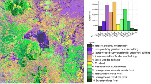
Compared to the vegetation structure composition maps generated using the FCD transformation, all maps derived using the RDF classification showed consistency in terms of the spatial distribution of each class. There is no significant difference between the general categorizations generated in this RDF classification map. Moreover, the gradation looks smooth on one side, but the appearance of several classes is more solid. This appearance is prominent for the classes of water bodies (Lake Rawa Pening), coffee and cocoa plantations, rubber plantations, and teak forests. However, the FCD transformation-based map looks better in differentiating urban/built-up area with very sparse vegetation (Class FCD 1) from other urban areas which are more vegetated (Class FCD 2). The suburb areas which consist of buildings and homestead garden are also correctly categorized as Class FCD 3. On the other side, the RDF algorithm could not correctly classify them since all urban building and the associated vegetation are classified as class FCD 2. This is the case with all 40 RDF resultant maps.

The distribution of vegetation structural composition classes according to the landform units are presented in Table 3. According to the table, the FCD classes 9 and 10 are mostly found in volcanic cones and volcanic upper slopes. Actually, the volcanic cones mostly occupied by the FCD class 10 are the ones with lower elevation than 2000 m asl, due to the climatic requirements or suitability. Compared to the FCD transformation results, the distribution of vegetation structural composition based on RDF classification model is more correlated to the distribution of landform units. For examples, the FCD class 0 (which is associated with barren land or built-up areas) are mainly found in very steep slopes, urban areas, as well as agricultural land. The FCD classes of dense vegetation (classes 8, 9 and 10) are mainly found in volcanic upper and middle slopes, as well as the old and highly dissected hills with pyroclastic.

Table 3. Distribution of FCD classes according to the Landform units (in hectares), based on RDF classification.

	FCD 0	FCD-1	FCD-2	FCD3	FCD-4	FCD-5	FCD-6	FCD-7	FCD-8	FCD-9	FCD10	TOTAL(ha)
Volcanic cone	2.34	90.3	73.65	157.11	578.01	78.51	9.15	352.8	370.23	218.67	199.65	71014
Volcanic upper slopes	19.47	160.47	370.29	436.47	1114.35	389.22	327	1489.95	749.01	425.7	296.19	192604
Volcanic middle slopes	55.29	180.03	875.97	1107.42	1582.32	268.62	572.82	696.15	264.69	53.82	50.4	190251
Volcanic footslope, highly dissected	0.96	30.21	67.98	71.94	375.18	5.7	59.61	65.37	41.28	2.4	0.03	24022
Volcanic footslopes – moderately dissected	249.93	473.22	1333.62	934.86	1167.54	254.04	674.85	857.34	10.23	5.61	0.18	198714
volcanic footslope – slightly dissected	190.92	439.32	1034.1	431.76	446.79	187.71	159.24	468.99	0.66	0.87	0	112012
Old, volcanic hill – highly dissected	0.24	1.92	13.47	12.87	44.31	10.05	15.42	24.69	4.11	1.05	0.03	4272
Old, highly dissected hills with pyroclastic materials	13.47	124.35	330.24	221.31	1251.27	133.2	368.85	815.58	1179.78	16.05	1.44	148518
Old, moderately dissected hills with pyroclastics	179.13	362.82	1907.37	1421.94	1429.23	341.22	919.74	722.76	9.93	2.79	0.27	243240
Structural hills with limestone sedimentary rocks	46.32	156.48	1223.34	324.69	146.43	43.77	89.28	512.43	0.15	0.33	0.03	84775
Lacustrine plain	520.5	577.38	109.53	125.79	53.4	26.28	22.14	53.76	0	0.12	0	49630
Total area	1278.57	2596.5	7339.56	5246.16	8188.83	1738.32	3218.1	6059.82	2630.07	727.41	548.22	39571.56

3.4. Accuracy assessment and comparison

Accuracy assessment of the results obtained using FCD transformation and RDF classification were undertaken using a set of polygons representing independently collected features in the field with the aid of high-spatial resolution imagery. We overlaid all generated maps with the field reference polygons to create accuracy assessment using confusion matrix. This study found that the FCD transformation result achieved 69.32% overall accuracy (Kappa = 0.6519), while the RDF-based classification results obtained various accuracy levels, ranging from 70.76% overall accuracy (Kappa = 0.6747) to 75.19% overall accuracy (Kappa = 0.7235). These accuracy values of the RDF classification results were obtained from 40 classified images, which were also computed with respect to their OOB accuracies. In addition, we also used the classification result of maximum likelihood algorithm as a comparison.

In short, among three different models generated using FCD transformation, RDF classification, and maximum likelihood classification, the machine learning-based RDF performs the best accuracy, while the maximum likelihood provides the worst. The RDF classification was run using 40 combination representing various number of split (Mtry) and number of trees (Ntree). With the RDF as a modification of Random Forest algorithm, there is no pruning so that all trees were used, as explained by Eastman (2019). Although the RDF classification delivered various accuracy levels, the lowest one still higher than that of FCD transformation result and maximum likelihood-based classified map. Moreover, the visual appearances of all RDF classification results show similar pattern, which do not exhibit the clear difference when observed visually at small scales.

It is also important to note that the OOB accuracy do not directly correlate with the overall accuracy that is computed using independent dataset. As shown in Figure 8, 40 classification results generated using RDF algorithm were assessed using OOB accuracy, Overall accuracy, as well as Kappa. We compared the results by grouping them into different number of splits and number of trees. Generally speaking, the OOB accuracies are low (0.69) when the number of splits are also low, which means that the algorithm only use less number of input variables (in this case, the input spectral bands). It gradually increases with the larger number of splits and reaches the highest one at 0.72 with the number of splits of five and six. However, the overall accuracies could reach the highest one (75.16 and 75.19) at the smaller number of splits, i.e. two, and at the medium number of trees, i.e. 200 and 250. After that, the overall accuracy gradually decreases with the larger number of trees, even though the smallest number of trees that were used here, i.e. 50 for both number of splits of three and five exhibit accuracy plunges as compared to the others. The Kappa is presented in % shows the same pattern as the overall accuracy.

Figure 8. OOB accuracy, overall accuracy and Kappa index obtained using RDF algorithm at various number of splits and number of trees.

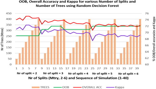
When the numbers of Mtry and Ntrees were compared, we found that their smaller numbers show better accuracy results than those with larger numbers. This was due to the several reasons, e.g. overfitting. Too large Mtry and Ntrees values may have caused the model to start overfitting the training data, which means that it learned the noise in the training data and finally generated poor generalization of new data. With smaller values of Mtry and Ntrees, the classification process is less likely to overfit and can better generalize to new data.

When we compared the result of RDF with the conventional maximum likelihood classification results, we found that the maximum likelihood-based vegetation structural composition map is less accurate, i.e. with overall accuracy of 60.81% and Kappa = 0.5665. It should be noted, however, that the sampling strategy for the maximum likelihood classification used the same sample dataset that was utilized by the RDF, which did not differentiate various types of barren land (e.g. dark open soil, light open soil, etc.). The samples also mixed-up various types of impervious surface (concrete rooftops, metal rooftops, asphalt surface) from the barren lands, leading to heterogeneous, not properly clustered features. Given that the maximum likelihood classifier works using assumption that every sample is spectrally homogeneous, and the pixel values are normally distributed (parametric classification approach), the low accuracy obtained is understandable. On the other hand, the RDF can work in a better way with this kind of samples, referring to FCD classification, which is probably due to the non-metric classification approach (Jensen 2015).

Apart from the numbers related to the accuracies obtained, a map-to-map comparison was carried out to see the resultant patterns obtained using two different models. We used the most accurate RDF-based map and the FCD map to compare, as presented in Figure 9. First, the distribution of the vegetation structural composition classes based on FCD transformation looks more random in character, while the one generated using RDF classification shows more clustered phenomenon. Second, the FCD transformation produced larger forested areas or tree-dominated structural composition classes than RDF. With the RDF, those classes are mainly found in rugged terrain with elevation less than 2000 m asl. Third, several categories related to specific ecosystem units were clearly misidentified using FCD. For example, the aquatic weed (Eichhornia crassipes) at the Rawa Pening Lake was miscategorized as FCD class 10 (extremely dense forest), although this vegetation type is a kind of floating herb. The FCD transformation also identified coffee and cocoa plants (just in the northeast of the lake) as heterogeneous vegetation with various densities, while the RDF algorithm classified them as denser wooded bushland. In the field, the coffee and cocoa plantations make up a combination between homogeneous shrub interleaved by shade trees of legumes (e.g. Leucaena leucocephala). The rubber plantation in the north of Salatiga was identified as FCD Classes 8 up to Classes 10 using FCD transformation, depending on its density, but these rubber trees were classified as woodland and woodland with multistorey trees by the RDF algorithm. Fourth, the FCD transformation identified urban areas as two categories: FCD Class 0 and Class 1 with respect to the percentage of associated vegetation. However, the RDF algorithm classified the urban areas more homogeneously as Class 2.

Figure 9. Comparison between vegetation structural composition maps generated using FCD transformation (left) and RDF machine learning classification (right).

The comparison shows that the FCD transformation is more sensitive to individual pixel characteristics in all involved bands, including shadow and temperature aspects. Therefore, a landscape containing many pixels with various types of vegetation would be identified individually regardless their adjacency. On the other hand, even though the RDF algorithm works like any other per-pixel classification, it can successfully classify pixels in more compact clusters. In addition, the misidentification using FCD transformation might be caused by the used of thermal band of Landsat in defining the thermal index (TI). Since the TI considers low temperature pixels are associated with dense vegetation, the lake water containing floating vegetation was identified as relatively dense vegetation. This study has tried to mask the water body using NDVI and SWIR band, but the vegetation content causes its values higher. The aquatic weed of Eichhornia crassipes was also treated similarly. Moreover, the shrubs and grass on the top of Mt Merbabu grow in the high-altitude soil, which are represented by low temperature pixels in the TI image. Therefore, their density was misidentified by the FCD transformation as denser vegetation structure.

Given that machine learning algorithms are usually able to accommodate input data in different domains, it is also interesting to consider that RDF or artificial neural network (ANN) as machine learning classifiers may be used to combine other spatial data like elevation, soil types and rainfall. Changes in mapping accuracy may be studied further in separate research, in order to analyze the sensitivity of particular input bands or other spatial variables to generate vegetation structural composition map.

4. Conclusions

This study showed that the deductive-deterministic-empirical model of FCD did not work well in a complex landscape with high-range altitudes, various landforms, and various types of vegetation interleaved by built ups areas and eutrophicating lake. The complex characteristics have led to the inaccurate information of the constituting indices. Meanwhile, the machine learning-based RDF algorithm could be used for classifying the vegetation structural composition used in FCD at moderately high accuracy, although it does not deliver ratio-interval values to be regrouped into discrete categories, like in the original FCD model. It directly classifies the categories using well defined samples referring to the FCD classes. A further study using different approaches in machine learning which makes use of terrain characteristics is recommended.

Acknowledgement

The authors would like to thank the Faculty of Geography, Universitas Gadjah Mada, for supporting this research. Comments and suggestions from the anonymous reviewers are also acknowledged.

Data availability statement

The data that support the findings of this study are available from the first author, PD, upon reasonable request.

Disclosure statement

No potential conflict of interest was reported by the authors.

References

- Abdollahnejad A, Panagiotidis D, Surovy P. 2017. Forest canopy density assessment using different approaches – Review. J For Sci. 63(3):107–116. doi: 10.17221/110/2016-JFS.
- Ahmed R. 2020. Temporal assessment of forest canopy density around Hojai-Diphu railway line in Assam, India. Int J Sci Technol Res. 9(03):3040–3043.
- Arjasakusuma S, Swahyu Kusuma S, Phinn S. 2020. Evaluating variable selection and machine learning algorithms for estimating forest heights by combining lidar and hyperspectral data. IJGI. 9(9):507. doi: 10.3390/ijgi9090507.
- Arjasakusuma S, Kusuma S, Mahendra W, Astriviany N. 2021. Mapping paddy field extent and temporal pattern variation in a complex terrain area using Sentinel 1-Time Series Data: case study of Magelang District, Indonesia. IJG. 17(2):79–88. doi: 10.52939/ijg.v17i2.1763.
- Bera B, Saha J, Bhattacharjee S. 2020. Estimation of forest canopy cover and forest fragmentation mapping using Landsat Satellite Data of Silabati river basin (India). KN J Cartogr Geogr Inf. 70(4):181–197. doi: 10.1007/s42489-020-00060-1.
- Biau G. 2012. Analysis of a random forests model. J Mach Learn Res. 13(1):1063–1095.
- Breiman L. 2001. Random forests. Mach Learn. 45(1):5–32. doi: 10.1023/A:1010933404324.
- Breiman L, Cutler A. 2005. Random Forests. Available at http://www.stat.berkeley.edu/∼breiman/RandomForests/.
- Chavez PS. Jr., 1996. Image-based atmospheric corrections revisited and improved. Photogramm Eng Remote Sensing. 62(9):1025–1036.
- Congalton RG, Green K. 2019. Assessing the accuracy of remotely sensed data - principles and practices. 3rd ed. New York: John Wiley & Sons.
- Costa H, Almeida D, Vala F, Marcelino F, Caetano M. 2018. Land cover mapping from remotely sensed and auxiliary data for harmonized official statistics. IJGI. 7(4):157–177. doi: 10.3390/ijgi7040157.
- Danoedoro P. 2019. Multidimensional land-use information for local planning and land resources assessment in Indonesia: classification scheme for information extraction from high-spatial resolution imagery. IJG. 51(2):131–146. doi: 10.22146/ijg.32781.
- Danoedoro P, Ananda IN, Kartika CSD, Umela AF, Indayani AB. 2020. Testing a detailed classification scheme for land-cover/land-use mapping of typical Indonesian landscapes: case study of Sarolangun, Jambi and Salatiga, Central Java. IJG. 52(3):327–340. doi: 10.22146/ijg.50080.
- Danoedoro P, Gupita DD. 2022. Combining pan-sharpening and forest cover density transformation methods for vegetation mapping using Landsat-8 Satellite Imagery. Int J Adv Sci Eng Inform Technol. 12(3):881–891. doi: 10.18517/ijaseit.12.3.12514.
- Danoedoro P, Gupita DD, Afwani MZ, Hadi HA, Mahendra WK. 2022. Preliminary study on the use of digital surface models for estimating vegetation cover density in a mountainous area. IJG. 54(3):333–342. doi: 10.22146/ijg.60659.
- Deka J, Tripathi P, Khan ML, Srivastava VK. 2019. Study on land-use and land-cover change dynamics in Eastern Arunachal Pradesh, N.E. India using remote sensing and GIS. Trop Ecol. 60(2):199–208. 2019, doi: 10.1007/s42965-019-00022-3.
- Eastman JR. 2019. Idrisi TerrSet – Guide to GIS and Image Processing. Clark Labs, Worchester, MA: Clark University.
- Fawagreh K, Gaber MM, Elyan E. 2014. Random forests: from early developments to recent advancements. Syst Sci Control Eng. 2(1):602–609. doi: 10.1080/21642583.2014.956265.
- Franklin J. 2013. Mapping vegetation from landscape to regional scales. In: van der Maarel E, Franklin J, editors. Vegetation ecology, 2nd ed. New York: John Wiley and Sons.
- Fu B, Wang Y, Campbell A, Li Y, Zhang B, Yin S, Xing Z, Jin X. 2017. Comparison of object-based and pixel-based Random Forest algorithm for wetland vegetation mapping using high spatial resolution GF-1 and SAR data. Ecol Indic. 73:105–117. doi: 10.1016/j.ecolind.2016.09.029.
- Giri CP. 2012. Remote sensing of land use and land cover: principles and applications. Boca Raton: CRC Press
- Gorelick N, Hancher M, Dixon M, Ilyushchenko S, Thau D, Moore R. 2017. Google Earth Engine: planetary-scale geospatial analysis for everyone. Remote Sens Environ. 202:18–27. doi: 10.1016/j.rse.2017.06.031.
- Hadi HA, Danoedoro P. 2021. Comparing several pixel-based classification methods for vegetation structural composition mapping using Sentinel 2A Imagery in Salatiga Area, Central Java. Proc. SPIE 12082, Seventh Geoinformation Science Symposium 2021, 120820T (22 December 2021). doi: 10.1117/12.2621965.
- Hartoyo APP, Prasetyo LB, Siregar IZS, Theilade I, Siregar UJ. 2019. Carbon stock assessment using forest canopy density mapper in agroforestry land in Berau, East Kalimantan, Indonesia. Biodiversitas. 20(9):2661–2676. 2019, doi: 10.13057/biodiv/d200931.
- Ho TK. 1995. Random Decision Forests. Proceedings of 3rd International Conference on Document Analysis and Recognition, 1995, pp. 278–282, vol.1, doi: 10.1109/ICDAR.1995.598994.
- Himayah S, Danoedoro, P, Hartono. 2016. The utilization of Landsat 8 multitemporal imagery and forest canopy density (FCD) model for forest reclamation priority of natural disaster areas at Kelud mountain, East Java. IOP Conf Ser: Earth Environ Sci. 47(1):012043., doi: 10.1088/1755-1315/47/1/012043.
- Huggett R, Cheesman J. 2002. Topography and the Environment. Harlow: Prentice Hall.
- International Tropical Timber Organization (ITTO). 1997. Utilization of Remote Sensing in Site 22 Assessment and Planning for Rehabilitation of Logged-Over Forests. Project Report on PD 32193 23 Rev.2 (F): Rehabilitation of Logged-Over Forests in Asia/Pacific Region, Sub-Project III.
- International Tropical Timber Organization (ITTO)/JOFCA. 2003. FCD-Mapper Ver.2 User Guide, Semi-Expert Remote Sensing System for Canopy Density Mapping.
- Ismail M, Danoedoro, P, Hartono. 2017. The application of forest cover density (FCD) model for structural composition of vegetation changes in part of Lore Lindu National Park, Central Sulawesi Province. IOP Conf Ser: Earth Environ Sci. 98(1):012056., doi: 10.1088/1755-1315/98/1/012056.
- Jensen JR. 2015. Introductory digital image processing – a remote sensing perspective. 4th ed. Englewood Cliffs, NJ: Prentice Hall.
- Küchler AW, Zonneveld IS. 1988. Vegetation mapping. Dordrecht: Kluwer. doi: 10.1007/978-94-009-3083-4.
- Mohammadpour P, Viegas DX, Viegas C. 2022. Vegetation mapping with random forest using Sentinel 2 and GLCM texture feature—a case study for Lousã Region, Portugal. Remote Sens. 14(18):4585.doi: 10.3390/rs14184585.
- Ohno K. 1991. A vegetation-ecological approach to the classification and evaluation of potential natural vegetation of the Fagetea crenatae region in Tohoku (northern Honshu), Japan. Ecol Res. 6(1):29–49. doi: 10.1007/BF02353868.
- Pratama LDY, Danoedoro P. 2020. Above-ground carbon stock estimates of rubber (hevea brasiliensis) using Sentinel 2A imagery: a case study in rubber plantation of PTPN IX Kebun Getas and Kebun Ngobo, Semarang Regency. IOP Conf Ser: Earth Environ Sci. 0(1):012087.
- Piranti A, Waluyo G, Rahayu DRUS. 2019. The possibility of using Lake Rawa Pening as a source of drinking water. J Water Land Dev. 41(1):111–119. doi: 10.2478/jwld-2019-0034.
- Rikimaru A, Roy PS, Miyatake S. 2002. Tropical forest cover density mapping. Trop Ecol. 43(1):39–47.
- Salsabila HN, Danoedoro P. 2021. The effect of atmospheric and topographic corrections on the vegetation density mapping using several vegetation indices: a case study in Arjuno-Welirang volcanoes. East Java. Seventh Geoinformation Science Symposium 2021. 12082, 279–284.
- Smith PF, Ganesh S, Liu P. 2013. A comparison of random forest regression and multiple linear regression for prediction in neuroscience. J Neurosci Methods. 220(1):85–91. doi: 10.1016/j.jneumeth.2013.08.024.
- Sukarna RM. 2008. Aplikasi Model Forest Canopy Density Citra Landsat 7 ETM untuk Menentukan Indeks Luas Tajuk (Crown Area Index) Dan Kerapatan Tegakan (Stand Density) Hutan Rawa Gambut Di DAS Sebangau Provinsi Kalimantan Tengah. Maj Geogr Indones. 22(1):1–21.
- van Bemmelen RW. 1949. The Geology of Indonesia. The Hague: V.F.A. Government Printing Office.
- van Gils H, van Wijngaarden W, Huizing H, van der Zee D. 1990. Land Ecology and Land-use Survey. Enschede: International Institute for Aerospace Survey and Earth Sciences.
- Xue J, Su B. 2017. Significant remote sensing vegetation indices: a review of developments and applications. J Sensors. 2017(17):1–17. doi: 10.1155/2017/1353691.
- Zaehringer JG, Llopis JC, Latthachack P, Thein TT, Heinimann A. 2018. A novel participatory and remote-sensing-based approach to mapping annual land use change on forest frontiers in Laos, Myanmar, and Madagascar. J. Land Use Sci. 13(1-2):16–31. doi: 10.1080/1747423X.2018.1447033.