Predictions of land use/land cover change, drivers, and their implications on water availability for irrigation in the Vea catchment, Ghana

Abstract

Assessment and prediction of land use/land cover change using spatiotemporal data are of great importance for better environmental monitoring, land use planning, and management. Therefore, the objective of this study is to predict LULC change, its driving factors and impact on water availability for irrigation in the Vea catchment, Ghana. CA-Markov model was used to predict land-use changes in 2038 and 2054. Terrset geospatial monitoring and modeling system software was used to run the model. The Relative Importance Index was used to identify major drivers of the LULC change. The results showed an increase in cropland from 181 km² in 2038 to 183 km² in 2054 at the expense of grassland and mixed vegetation/forest, which are expected to decrease from 51–50 km² and 73–71 km², respectively. Population growth and agricultural expansion are among the leading drivers of LULC change in the Vea catchment. The CA-Markov model shows a continued increase in anthropogenic land uses, negatively affecting irrigation water availability and landscape sustainability. These results provide a foundation for sustainable land use governance through responsible planning and management of land and water resources by considering trade-offs between LULC change and water availability for irrigation in the Vea catchment.

Keywords:

• CA-Markov model
• Ghana
• land use/land cover
• land change modeler
• Vea catchment

1. Introduction

Changes in land use/land cover (LULC) are one of the most challenging and persistent drivers of environmental change. It is increasingly identified as an important cause of environmental change across all geographic and temporal dimensions. Several interconnected earth systems are influenced by humans and alter the regular provisions of the global natural environment. LULC change has a detrimental effect on the sustainability of the global environment and is perhaps the most pressing concern in many parts of the world (Sleeter et al. 2013). Over the past 300 years, LULC change around the world has been ranked by gains in agriculture and declines in other areas (forests, grasslands, water and wetlands) (Chisanga et al. 2022). Globally, every year, millions of hectares of forests are burned. For example, FAO (2020) estimates that around 420 million hectares of forest land globally is degraded with 10 million hectares of forest cleared annually. Since 1990, as with the rest of the world, in Africa, the extent and intensity of natural resource extraction has led to significant changes in land properties (Govender et al. 2022). According to a report by FAO (2011), about 27.4% of Africa’s land area (nearly 500 million hectares) is degraded. An extensive review of LULC in Africa found that agricultural land expansion, influenced by population growth, is the main driver of LULC change at the expense of forests (Govender et al. 2022). Rapid changes in the LULC are recognizable in Ghana. Ghana’s protected forest reserves experienced average annual deforestation rates of 0.7, 0.5, 0.4 and 0.6%, respectively, over the periods 1990–2000, 2000–2005, 2005–2010 and 2010–2015 (Springgay et al. 2019).

Predicting changes to LULC is a step towards ensuring effective land use planning and sustainable management of land resources and is routinely used for various suitability measures as an indicator of human impact on land change processes (Gashaw et al. 2017). Remote sensing (RS) and geographic information systems (GIS) are the most popular tools used in LULCC research. RS detects and monitors land use at various levels, from which land cover information can be extracted (Hua 2017a, b). while GIS provides a flexible environment to collect, store, display and analyze digital data required for change detection and subsequent prediction (Shawul and Chakma 2019). Since there are many models for simulating changes in LULC, their complexity with respect to stochastic change and the dynamic nature of natural and socioeconomic variables must often be considered (Abdurahman et al. 2023). As reported by Yirsaw et al. (2017), several models are based on agents (Xie et al. 2007), CLUE (Han et al. 2015), mobile automaton (CA) and Markov chains. A multidisciplinary model that combines elements of different modeling techniques has been proposed to develop predictions of future LULC change (Olmedo et al. 2015). A CA Markov model is a combination of cellular automata and transition probability matrices generated by mapping between two different images (Nadoushan et al. 2015). Markov chain analysis is a useful tool for modeling land use and land cover change (LUC) when the changes and processes in the land use layer (LUC) are difficult to describe. In addition, the use of CA-Markov model in LULC change studies has the advantage of its dynamic simulation capabilities; high efficiency with data, simple calibration; and the ability to simulate multiple land cover and complex patterns (Khawaldah et al. 2020; Munthali et al. 2020). Therefore, we used the CA-Markov model with the Terrset geospatial modeling and monitoring system software to improve the simulation of complex land cover in the Vea catchment.

The Vea catchment is a sub-catchment of the White Volta basin and source water for the Vea irrigation reservoir. Historically, it was a mosaic landscape consisting of large natural forests, woodlands, and savannah grasslands. The landscape of the catchment area is suitable for agriculture, settlements, and mining. Due to its favorable landscape, the catchment has been exposed to LULC changes as a result of population growth and the associated expansion of agricultural land. Little has been done by the regional environmental protection authority to change this situation through the preservation of natural forests. Regardless of the efforts made, the catchment is experiencing noticeable environmental problems such as land degradation, overgrazing, and deforestation resulting in a decline in land productivity. This phenomenon necessitates the generation of scientific information regarding changes in LULC, associated potential drivers, and future projections to develop appropriate land use plans. Therefore, the modeling of changes in LULC is at the center of current scientific research to make informed planning decisions for the development of green development policies and strategies. The purpose of this study was to address the following questions: (1) Which LULC classes have changed to other classes in the study area during the last 24 years (1998–2022)? (2) Which LULC classes will be changed to other land uses in 2038 and 2054? (3) What are the possible drivers of LULC change in the study area? (4) How does LULC change affect future water availability for irrigation in the study area? This study is crucial to provide empirical evidence of previous and future LULC change patterns by the driving factors of change and their impact on the availability of water for irrigation for natural resource managers, ecologists, and decision-makers to develop a land use plan that affects the sustainable land management of the studied landscape.

2. Materials and methods

2.1. Description of the study area

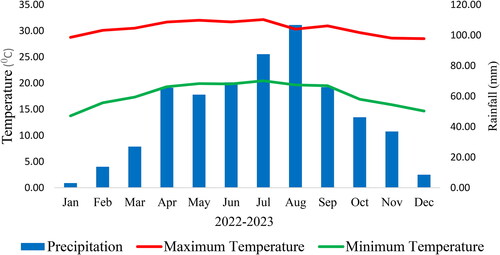
The Vea catchment is between latitudes 10°30′ and 11°00′N and longitudes 1°12′W and 0°50′E (Figure 1). The catchment mainly covers Bongo and Bolgatanga districts in Ghana and south-central Burkina Faso (Larbi et al. 2019). The catchment area consists of three agroecological zones in the semi-arid zone with an average yearly rainfall of about 956 mm, and its peak is in August; the basin has a unimodal rainfall regime from May to October. The temperature is generally higher than the average annual temperature of 28.9 °C, except for the wet months of July, August, and September. The rainfall pattern is shown in Figure 2. Potential evaporation exceeds yearly precipitation (Limantol et al. 2016). The Vea catchment has a relatively low topography with elevations between 89 and 317 m above sea level. LULC is mainly cropland, followed by grassland with mixed vegetation/forest. The primary economic activity of the inhabitants of this area is agricultural production (Larbi et al. 2019).

Figure 1. Map of the study area.

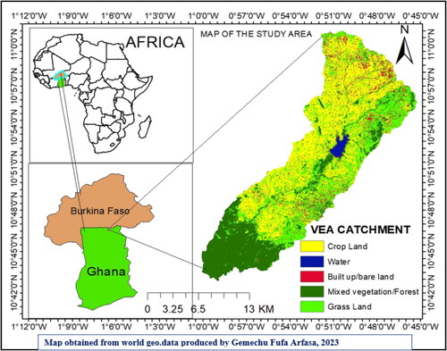
Figure 2. Monthly temperature and rainfall of Vea catchment.

2.2. Data sources and methods of acquisition

Satellite images were obtained from the United States Geological Survey (USGS) Data Portal (http://earthexplorer.usgs.gov). World Reference System "WRS", Path 194, Row 52, was applied to select the area of interest. To examine land cover changes in the Vea catchment, four Landsat scenes were captured between 1998 and 2022, each taken eight years apart. Images were taken in November with at least 5% cloud cover to reduce seasonal variation in vegetation and pattern variation. Google Earth Pro was used to reference and validate satellite images. A DEM (Digital Elevation Model) with a resolution of 30 m was obtained from the SRTM (Shuttle Radar Topography Mission) and was also used to collect spatial data. All data (images) are projected to the Universal Transverse Mercator (UTM) Zone 30 N projection system and the World Geodetic System-84 (WGS84) reference to ensure consistency between data sets during analysis. Data collection and other information for each Landsat scene are presented in Table 1.

Table 1. Sources and description of satellite data.

Sensor type	Date of acquisition	Cloud Cover (%)	Pixel resolution	WRS		Spectral resolution	Bands/ colour
				Path	Row
Landsat TM	06/11/1998	5	30 × 30	194	52/53	8	Multi-spectral
Landsat7 ETM+	09/11/2006	5	30 × 30	194	52/53	8	Multi-spectral
Landsat 8 (OLI)	23/05/2014	4	30 × 30	194	52/53	11	Multi-spectral
Landsat 8 (OLI)	16/05/2022	4	30 × 30	194	52/53	11	Multi-spectral

OLI: Operational Land Imager; ETM+: Enhanced thematic mapper, Thematic Mapper (TM).

2.3. Methods of data acquisition

Each Landsat scene’s acquisition dates and further details are displayed in Table 1.

2.4. Land use and land cover change assessment

2.4.1. Image pre-processing

Environmental resource data analysis system (ERDAS) Imagine version 2015 software is used for preprocessing operations. The most common image preprocessing methods are geometric and radiometric corrections that improve the quality of remotely sensed images for further analysis. Therefore, as suggested by Mohajane et al. (2018), all images for this study were geometrically corrected and rectified at level 1 (L1T). To reduce errors in the digital number of images and improve their interpretation, radiometric correction is applied (Hoque et al. 2021; Nath et al. 2023). The image processing chain was also performed using the open source software Quantum GIS (QGIS version 3.10) (QGIS, https://qgis.org/en/site/). Atmospheric correction was applied using a semi-automatic classification plugin (Mohajane et al. 2018) was done based on the Dark Object Downloading (DOS) algorithm (Abdurahman et al. 2023). In this study, radiometric correction was applied to the TM, ETMþ and OLI images for the years 1998, 2006, 2014 and 2022. The conversion process was performed for each of the TM, ETM + and OLI items at a resolution of 30 m. 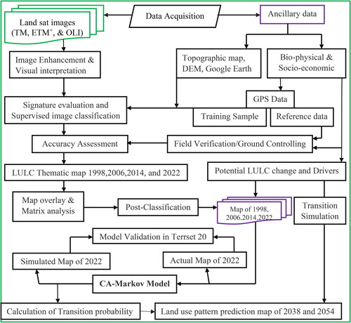For all images, calibration was obtained by converting raw digital numbers (DN) to sensor spectral radiance using Equation (1)(1) $$L\mathrm{\lambda }=(L\mathrm{\lambda }\max -\text{Lλmin})/(\text{QCALλmax}-\text{QCALλmin})\times (\mathrm{DN}-\text{QCALλmin})+\text{Lλmin}$$(1) . A flowchart with the methodology followed in this study is presented in Figure 4. All bands of TM, ETM + and Operational Land Imager (OLI) were considered for layers stacking. After stacking the satellite, data/images were clipped to a subset of the case study area which is 306 km² in order to focus on the relevant data. (1) $$L\mathrm{\lambda }=(L\mathrm{\lambda }\max -\text{Lλmin})/(\text{QCALλmax}-\text{QCALλmin})\times (\mathrm{DN}-\text{QCALλmin})+\text{Lλmin}$$(1) where Lλ is the spectral radiance at the sensor’s aperture in mW/(cm2 ·sr·µm); DN is the digital number of the quantized calibrated pixel value; Lλmax is the maximum spectral radiance that is scaled to QCALλmax; Lλmin is the minimum spectral radiance that is scaled to QCALλmin; QCALλmax is the maximum quantized calibrated pixel value in DN (corresponding to Lλmax); and QCALλmin is the minimum quantized calibrated pixel value in DN (corresponding to Lλmin). After this conversion, the radiance is converted into top-of-atmosphere (TOA) reflectance using Equation (2)(2) $$P=\frac{\pi L{d}^2}{\mathit{ESun}\text{λcosθ}}$$(2) : (2) $$P=\frac{\pi L{d}^2}{\mathit{ESun}\text{λcosθ}}$$(2) where q ¼ Unitless planetary reflectance, L ¼ Spectral radiance at sensor aperture, d ¼ the Earth-Sun distance which is on the date of imaging, ESun ¼ Mean solar exoatmospheric irradiance, $\pi =$ Mathematical constant equal to ∼3.14159 [unitless], $\mathrm{\theta }\mathrm{s}=$ Solar zenith angle [degrees]

2.4.2. Image classification

To classify LULC categories, training sites were randomized and used to locate training pixels for each LULC classes. Training sites supported high-resolution images from Google Earth for current imagery generated by GPS readings. For old historical images, Training sites were assigned using visual image interpretation, information from local elders, and local knowledge from researchers. At the evaluation stage, signature editions are made by deleting, merging or renaming until the most satisfactory results are achieved. Supervised Maximum Likelihood Classification (MLC) has been widely used to obtain LULC information from multidimensional raster images through the process of image interpretation and classification (Govender et al. 2022; Nageswaran et al. 2022; Abdurahman et al. 2023). This is mainly because the classification errors are minimized by considering the variance-covariance within the class distribution and combining the spectral class signatures of individual components to obtain them for reasonable classes. It is preferred because of its availability and the fact that it does not require long training. Therefore, this study uses MLC with field integration and Google Earth verification, a popular image classification method (Abdurahman et al. 2023; Nath et al. 2023). To monitor LULC change, it is necessary to have at least two periods of data for comparison (Mohajane et al. 2018). Therefore, the LULC map was created by Landsat (TM, ETMþ and OLI) for the years 1998, 2006, 2014 and 2022. Five LULC classes were identified using field observations, expert opinion, and photographs of specific locations (Table 2). GPS was used for subsequent classification. Therefore, field visits were conducted for field testing of uncertain land covers to further refine the LULC classification. Multi-temporal grid layers were then generated and their corresponding statistics compared to LULC change estimates.

Table 2. Description of LULC classes (Larbi et al. 2019).

LULC categories	Description
Cropland	Areas used for crop cultivation
Grassland	The land mostly covered with grasses
Mixed vegetation/forest	Land covered with dense trees, mixed forests, and plantation forests.
Waterbody	Areas covered with standing or moving water
Built-up/bare land	Areas of human settlements, roads, artificial surfaces, and bare soil

2.4.3. Accuracy assessment

Accuracy assessment tells us to what extent the ground truth is depicted on the equivalent classified image (Abbas and Jaber 2020). The classification accuracy assessment provides the degree of reliability of the results and subsequent change detection (Brown et al. 2020). The classified map was compared to ground truth data to assess accuracy. For 2006 and 2014, the reference points were collected from Google Earth, original Landsat imagery, interviews, group discussions, previous reports and maps. For the 2022 image, Google Earth, field observations, original Landsat imagery, interviews and group discussions of random reference points in different LULC types from the field survey using GPS were recorded.

The most common and effective way to measure classified image accuracy from remotely sensed imagery is an error/confusion matrix (Visa et al. 2011). The confusion matrix provides user accuracy, producer accuracy, overall accuracy and kappa statistics. Kappa coefficient was determined by using Equation (3)(3) $$K= \frac{N\sum r i=1\mathit{\text{xii }}- \sum r i=1 (xi+ \times x+1)}{N2 - \sum r i=1(xi+ \times x+1) }\mathrm{*}100$$(3) (Rwanga and Ndambuki 2017). According to (Foody 2020), a kappa coefficient value below 0.4 indicates poor agreement, a value between 0.4 and 0.8 represents moderate agreement, and a value above 0.8 indicates strong agreement. (3) $$K= \frac{N\sum r i=1\mathit{\text{xii }}- \sum r i=1 (xi+ \times x+1)}{N2 - \sum r i=1(xi+ \times x+1) }\mathrm{*}100$$(3) (4) $$K= \frac{\left(\text{Total * sum of correct}\right)\mathrm{ }-\text{ sum of all the }\left(\text{row total * column total}\right)}{\text{Total squared }-\text{ sum of all the }\left(\text{row total * column total}\right)}$$(4) where r is the row number in the matrix, xii is the number of observations in row i and column i (the diagonal elements), x + i and xi + are the marginal totals of row i and column j, respectively, and N is the number of observations.

2.4.4. Change detection

Due to the availability of large storage data sets, a number of numerical change detection algorithms and methods have been developed and studied over the past decades to estimate and detect LULC changes (Lu et al. 2014). These methods and procedures have been thoroughly reviewed, with excellent descriptions and summaries provided. The most common approaches for change detection include image contrast, image segmentation, PCA, CVA and post-classification comparison (Hansen 2022). Recently, there has been much debate about the application of machine learning algorithms to remote sensing images (Friedenthal et al. 2018). In this study, we investigated and detected changes in the spatial extent and model of the study area through a change detection method based on QGIS, which combines GIS and ERDAS images. For each type of LULC, the area in km2 and the percentage change for the periods 1998–2006, 2006–2014, 2014–2022 and 1998–2022 were calculated to analyze land cover change in the study area. Although the LULC statistics are calculated differently, the change in LULC over the four time periods is based on the difference between the years 1998, 2006, 2014 and 2022. Magnitude of Change (MC), Percentage change (PC) and rate of change (ARC) of the classified images were calculated based on the following equations: (5) $$MC\left({\mathrm{km}}^2\right)=Af-Ai$$(5) (6) $$PC\left(\%\right)=\frac{Af-Ai}{Ai}*100$$(6) (7) $$\mathit{ARC}\left({\mathrm{km}}^2{\mathrm{year}}^{-1}\right)=\frac{Af-Ai}{n}$$(7) (8) $$\left(\text{Rate of change}\left(\mathrm{R}\right)\left(\frac{\mathrm{ha}}{\mathrm{yr}}\right)=\frac{\text{Area final year}-\text{Area initial year}}{\text{area initial year}}\times 1/\left(\text{time interval}\right)\times 100)\right)$$(8) where Ai is the class area (km2) at the initial time, Af is the class area (km2) at the final time, and (n) is the number of years of the study period. Loss = Row total - diagonals of each class. Gain = column total – diagonals of each class. Net change = gain-loss. Net persistence = Net change/diagonals of each class

2.4.5. Annual rate of change analysis

The difference between the final year and the initial year, determining the magnitude of change between corresponding years, will be divided by the initial year and period to obtain the annual rate of change for each land use type. For determining the spatiotemporal size and rate of change in LULC categories (Equation 9(9) $$\mathrm{ARC}\left(\%\right)=\frac{\mathrm{Fy}\text{-}\mathrm{Iy}}{\text{Iy*t}}\mathrm{*}100$$(9) ): (9) $$\mathrm{ARC}\left(\%\right)=\frac{\mathrm{Fy}\text{-}\mathrm{Iy}}{\text{Iy*t}}\mathrm{*}100$$(9) where ARC is the annual rate of change in LULC categories. Iy and Fy are the initial and final year areas, respectively, and t is the time interval.

2.5. Land use/land cover change drivers

Changes in LULC are driven by natural and human activities (Xing et al. 2018). Large-scale global and regional changes in LULC have important implications for many ecological aspects. If the engines of change remain in the past, it is safe to believe that they will remain influential forces in the future (Leta et al. 2021). Topographic and distance driver variables have been used in LULC change modeling studies. Elevation, slope, distance from roads and distance to building were considered as potential driver variables. Road and river area distances were set as dynamic variables to express the differential distance as it changes over time.

2.6. Change analysis and modeling

2.6.1. Post-classification change analysis using the land change Modeler

Various modeling tools have been used to analyze LULC dynamics, with each tool offering different levels of accuracy (Hamad et al. 2018). Land Change Modeler (LCM), Cellular Automata (CA), and CA-Markov are embedded in Terrset software and are commonly used tools for LULC change modeling. For short-term forecasts, mostly ten years or less, for short-term forecasts, typically ten years or less, LCM provides predictive accuracy in LULC change analysis (Roy et al. 2014). In addition, LCM provides more accurate results compared to other models that project LULC changes based on supervised classification due to the robustness of the multi-layer perceptron-neural (MLP) network used in LCM (Pérez-Vega et al. 2012). These reasons guided the LCM decision to predict LULC changes in the Vea catchment for the 2054 horizon. LULC change analysis and scenario maps of the Wea Basin were generated in LCM using change analysis, transition potential modeling, model validation and change prediction (Figure 3). The model evaluates the change of LULC between two sets of images with different data, the same legend and the same spatial features, and presents the results of the changes in a chart and map form (Megahed et al. 2015). In this study, LULC changes for four time periods (1998–2006, 2006–2014, 2014–2022 and 1998–2022) were performed using the post-classification comparison method, a widely used approach to detect LULC changes (Mahmoud and Alazba 2016). LULC change analysis was performed using the change detection module in LCM, which provides information on the gain and loss of each LULC class, the net change, which is the difference between the gain and loss of each class, the contributions to the net change. Each class and transition intervals between each LULC class that occurred between two different dates (Larbi et al. 2019).

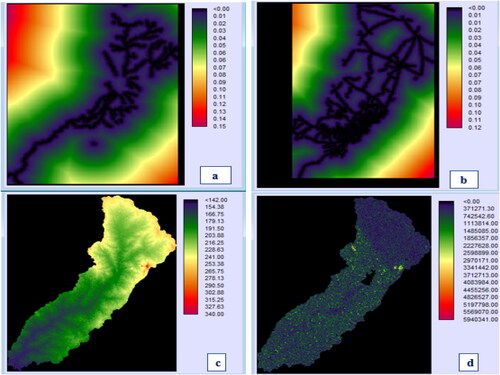
Figure 3. The suitability maps and input data: Distance from river (a), distance from road (b), DEM (c), and slope (d), are the input data. Source: NASA Shuttle Radar Topography Mission (SRTM) (2013). Shuttle Radar Topography Mission Global. Distributed by Open Topography. https://doi.org/10.5069/G9445JDF.

2.6.2. Modeling of transition potentials using the multilayer perceptron neural network

The LULC maps of the year (2006–2014 and 1998–2014) were used as inputs to create the transitions. Using the change analysis module, dominant transitions (grassland to cropland, forest/mixed vegetation to cropland, and forest/mixed vegetation to grassland) were identified, which were used to create potential transition maps for modeling by setting a threshold of 1000 hectares. The change maps were used to determine the probability of conversion from other classes to cropland. The LCM uses logistic regression, Sim Weight and a multi-layer perceptron neural network (MLP) as modeling algorithms to model transition variables. In this study, the MLP neural network was used to construct the transition potential maps. The MLP is extensively extended and requires no user intervention, with the ability to model multiple transitions simultaneously and also to model non-linear relationships. The MLP neural network operates as a feedforward artificial neural network (ANN) model with a unidirectional flow of data through hidden layers in between. Neural network training is based on a supervised training algorithm, which is a common method for training ANNs. The transition potential maps for the LULC changes were generated with an MLP accuracy rate (89%), which is within the acceptable range.

2.6.3. LCM validation and change projection

After the model is created, the simulation map must be checked for correctness of the prediction. Therefore, model validation is one of the important stages of land use prediction. The validation module includes a comparative evaluation of the simulated and real maps based on the Kappa index. However, it differs from the traditional kappa statistic in that it divides the validation into many components, each with a specific kappa pattern such as Klocation, Kno, Kstandard, etc. The results of the model were compared with the current or actual land use map. The comparison of the projected LULC map representing the LULC in 2022 with the actual LULC (2022 map) is based on the Index of Agreement (KIA) approach, which is often used to validate predictions of LULC change (Eastman and Toledano 2018). Before the CA Markov model can be applied to estimate the next 32 years. For this purpose, the validation module available in Terrset Software must be used.

2.6.4. Simulation and prediction of land use/cover changes

2.6.4.1. Markov-chain model analysis

The Markov chain model is a unique and widely used land use and land cover modeling tool that represents LULCC as a stochastic process. In a Markov system, the future state of the crop system is modeled based on the immediate state of progress. The transition of the system from one state to another is a transition, and the probability associated with that state transition is called the transition probability. The initial estimates of $\mathit{pij}$ can be computed as (10) $${\mathit{P}}_{\mathit{ij}}={\mathit{P}}_{\mathit{ij}}/{\mathit{N}}_{\mathit{t}}(\mathit{ij}\dots 1,2,3,\dots .\mathit{m})$$(10) where $\mathbf{Nij}$ is the number of units transitioned from the state i to state j, $\mathbf{Ni}$ is the number of units in state i.

Therefore, the basic hypothesis of the Model simulation process mainly produces a Land Use area transfer matrix and a probability transfer matrix to predict land use change. The Markov Chain Model is described as a set of states, S=(S_1, S_2, S_3,…S_n) assuming that the current state is〖S〗_t and then, it changes to state S_j at the next step with a probability denoted by transition probabilities P_IJ Thus, the state S_(t + 1) in the system determined by former stage S_t in the Markov Chain using the following formula (Chang et al. 2018); (11) $${\mathbf{P}}_{\mathbf{ij}}=\left[\begin{array}{ccc}{\mathbf{P}}_{\mathbf{ll}}& \cdots & {\mathbf{P}}_{\mathbf{ln}}\\ ⋮& \ddots & ⋮\\ {\mathbf{P}}_{\mathbf{nl}}& \cdots & {\mathbf{P}}_{\mathbf{nn}}\end{array}\right](0\le {\mathit{P}}_{\mathit{ij}}\le \mathit{l} \mathit{and}\sum \mathit{Pij}=\mathit{li},\mathit{j},\dots ,\mathit{n})$$(11) $${\mathbf{S}}_{\mathbf{t}+1}={\mathbf{P}}_{\mathbf{ij}\mathrm{ }}\times \mathrm{ }{\mathbf{P}}_{\mathbf{t}}\dots .$$ where $P_{ij}$ is the state transition probability matrix and n are the land represents the number of land use type; S is land use status, t; t + 1 is the time point. In this study, Markov chain analysis was conducted in three periods; 1998–2006, 2006–2014, 2014–2022 and 2022–2054. In this way, the matrix of the transition area of land use and the transition probability matrix for the current periods were determined.

2.6.4.2. Cellular automata (CA)

The CA model is a change model with local interaction that reflects the evolution of the system, where space and time are treated as discrete entities, and space is often represented as a regular two-dimensional grid. The temporal and spatial complexity of land use land cover systems can be well modeled by properly specifying transition rules in CA models. CA modeling provides important information for understanding theories of forest cover, such as the evolution of forms and structures (Zhang et al. 2008). Cellular Automata is a bottom-up dynamic model within a spatio-temporal computation. It is discrete in space-time and the state can perform complex time-space modeling. The data for each cell in the St + 1 state is determined by the cell itself and its neighboring cells in the St state, which means that changes in the cell are handled according to the rules. It mainly consists of cells, cell space, neighbor, rule and time. The CA model filter identifies neighbors (Zhou and Chen 2018). The smaller the distance between the original cell and its neighbor, the greater the weighting factor. The weight factor is combined with the transition probability to predict the state of neighboring network cells. See above that land use changes are not entirely random decisions. In this study, the cellular automata network represented each land use cell, and each network had 8 neighboring cells; Cell status represented the type of land use of the cell; the time interval is 24 years. To track land use transitions, the maximum transition probability rule and the hysteresis rule are valid. If a cell is assigned a land use type, the cell will not change to other land use types during the simulation period (Aburas et al. 2016; Vázquez-Quintero et al. 2016; Gharaibeh et al. 2020). (12) $$St+1=f(St,N)$$(12) where S is the set of states of the finite cells. t and t + 1 are different moments; N is the neighborhood of cells; and f is the local space transformation rule (Figure 4).

Figure 4. Methodological flowchart land use land cover change detection and modeling.

3. Result and discussion

3.1. Status of land use/land covers

Five LULC classes were identified for the period of 1998–2022 (Figure 5). In 1998, the grassland accounted for 54.8%, followed by mixed vegetation/forests (31.7%), cropland (10.9%), built-up areas (1.6%), and waterbodies (1.1%), which show minimal coverage of the Vea Catchment (Table 3). In 2006, grassland cover was about 39.7%, followed by mixed vegetation/forests (29.1%), while cropland, built-up area and waterbodies accounted for 26.2, 4 and 1.1%, respectively. In 2014, grassland covered about 32.6%, followed by mixed vegetation/forests (23.6%), cropland increased to 36.6%, and built-up area and waterbodies accounted for 6.1 and 1%, respectively. Grassland declined to 16.6% in 2022, mixed vegetation/forest decreased to 22.73%, and water decreased to 1.03%, whereas cropland and built-up area increased by 52.87 and 6.75%, respectively. In the entire study period, cropland and built-up areas significantly increased at the expense of forestland and grassland coverage, which decreased by 54–75.1 km² and 174.5–54 km² from 1998 to 2022 (Table 3).

Figure 5. LULC of 1998, 2006, 2014 and 2022 of the Vea catchment.

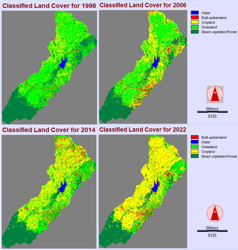
Table 3. Area of LULC class from 1998 to 2022 (area in km²).

LULC classes	1998		2006		2014		2022
	km2	%	km2	%	km2	%	km2	%
Water	3.5	1.1	3.46	1.1	3.43	1	3.41	1.03
Built-up and bare land	5.1	1.6	13.1	4	20.5	6.3	22.3	6.75
Grassland	181	54.8	131	39.7	107.6	32.6	54	16.6
Cropland	36.1	10.9	86.4	26.2	120.8	36.6	174.5	52.87
Mixed v./forest	104.5	31.7	96.2	29.1	77.8	23.6	75.1	22.73

3.2. LULC conversions analysis

The LULC change was performed by taking the initial year of 1998. Four LULC conversions were detected, that is, between 1998 and 2006, 2006 and 2014, 2014 and 2022, and 1998 and 2022. The conversion results revealed substantial losses and gains in LULC in the first (1998–2006), second (2006–2014), third (2014–2022) and fourth (1998–2022) study periods. For instance, grassland, mixed vegetation, and water bodies were converted to other LULC classes during the first, second, third, and fourth study periods. Grassland converted to other LULC classes by about 70.81 km² in 2006, 51.9 km² in 2014, and 58.4 km² in 2022. Mixed vegetation/forest converted to other land use land cover classes by 11.7 km² in 2006, 20.3 km² in 2014, and 6.29 km² in 2022. Cropland converted to other land use land cover classes by 11.58 km² in 2006, 46.1 km² in 2014, and 5.46 km² in 2022. Built-up area and bare land converted to other land use land cover classes by 0.45 km² in 2006, 8.1 km² in 2014, and 10.3 km² in 2022. While water converted to other land use classes by 0.15 km² in 2006, 0.01 km² in 2014, and 0.09 km² in 2022. Table 4 shows that three LULC classes registered a negative annual change between 1998 and 2022. Annual losses in the grassland, water, and mixed vegetation/forest classes were −0.15, −0.01 and −3.67 km², respectively. For the same time period, the annual rate of change (ARC) for these classes was −8.35, −2.58, and −3.5%, respectively.

Table 4. The annual rate of changes in km² and % occurred from 1998 to 2022.

Land use classes	1998-2006		2006-2014		2014-2022		1998-2022
	km2	%	km2	%	km2	%	km2	%
Water	−.05	−0.14	−0.004	−0.14	−0.001	−0.03	−0.01	−2.58
Built up	1.0	19.6	0.92	7.06	0.04	0.18	1.89	37
Grassland	−6.2	−3.45	−2.9	−2.23	−5.95	−5.53	−15.12	−8.35
Cropland	6.28	17.4	4.3	4.97	6.34	5.25	16.92	46.88
Mixed V./F	−1.0	−0.99	−2.3	−2.4	−0.34	−0.43	−3.67	−3.5

3.3. LULC change driver variables

Driver variables that affect change are based on spatial analysis and added to the model as static or dynamic components. The LULC prediction in the catchment is based on changing driver effects. In this study, both topography and proximity factors were selected to analyse LULC change. Selected driver variables were evaluated for their explanatory value using Cramer’s V and P values before entering the model (Table 5). Cramer’s’ V value does not provide convincing evidence that any particular variable explains land use change. Instead, it is a much easier tool to understand the importance of a variable in influencing change. Index probability is used to determine the relative frequency of pixels of different LULC types in different regions. Recommended in cases where Cramer’s V value is low. The result obtained is considered good in terms of probabilities. In this study, it was a quantitative measure of the frequency of variation between crops and other soils (also known as disturbance). Table 5 shows that variables such as elevation, slope, distance to the river, and distance to the road are considered useful variables for the transition. Variables such as slope have low Cramer’s V values, indicating that the influence of slope on LULC change in the study area is not important. Variables with good Cramer V values suggest that they are the most explanatory variables for the LULC change. All other variables were used to model the transition. Elevation and slope are considered to be the dominant topographic factors affecting LULC change. Topography affects the extent and extent of built-up areas, vegetation, mixed forests, and the conversion of grasslands into cropland. Qasim et al. (2013) found that deforestation decreases with increasing slope. In the lowlands, accessibility is the factor most closely associated with agricultural expansion. Other influencing factors, such as distance to rivers and distance to roads, also play an important role in land use change as they make it easier for people to access resources.

Table 5. Cramer’s V and p-value for each of the explanatory variables.

Driver variables	Cramer’s V	p-value
Distance from road	0.1391	0.0000
Distance from river	0.2158	0.0000
Elevation	0.2967	0.0000
Slope	0.0094	0.0000

3.4. Transition probability matrix (TPM)

The transition potential model evaluates the possibility of LULC transition from one layer to another based on the appropriate transition of the region and the presence of driving forces (Mahamud et al. 2019). TPM captures the probability that each land-use class shifts to another. The LULC change predictions are mined by the probability of the transition matrix (Muhammad et al. 2022). The model-generated transition probability matrices between LULC types in the periods 1999–2006, 2006–2014, 2014–2022 and 1998–2022 were presented in Tables 6–9, respectively. The spatiotemporal LULC change values between the previous and subsequent land cover maps were tabulated. Cross-tabulation is used to determine the degree of change and conversion between different land cover maps. In the cross-tabulation (Tables 6–9), the frequencies in bold according to the diagonal transition probability matrix confirm the probability of the LULC class remaining unchanged from the previous map to the land cover map. Cropland land has the highest area of 185.5 km² and is expected to remain as cropland from 1998 to 2022. The conversion of mixed vegetation/forest and grassland was the most important land use factor for arable land. The mean loss of the LULC category was observed from the water body to grassland and built-up/bare land. However, there has been minimal or no conversion to grassland and water on built-up/bare land. From 1998 to 2022, the biggest loss was the conversion of grassland to cropland by 185.5 km². The lowland areas of the catchment were covered with forests and grasslands before 2006 and even before 2014. Currently, due to the expansion of cropland, the area of grasslands and forests has decreased sharply. Recently, the expansion of built-up areas has been increasing continuously and at a faster rate. A study in China reported that urban built-up land expansion results from the conversion of cultivated land (Wu and Zhang 2012). Kafy et al. (2021) revealed that effective urban planning is necessary to address the multiple challenges and competing interests of urban environments due to the rapid increase in urban built-up area and the scarce land and water resources on the urban edge.

Table 6. Transition area matrix (km²) and accuracy assessment of the Vea catchment from 1998 to 2006.

LULC classes		2006						Producer accuracy (%)	User accuracy (%)
		Built up/bare land	Cropland	Grass land	Mixed v./forest	Water	Row total
1998	Built up/bare land	3.83	0.22	0.192	0.012	0.00	4.286	93.1	90
	Cropland	0.07	22.15	11.326	0.180	0.00	33.729	93.1	87.1
	Grass land	9.59	56.68	114.569	4.51	0.00	185.382	97.8	96.7
	Mixed V./forest	1.04	4.23	6.487	91.556	0.00	103.307	88.9	97.6
	Water	0.01	0.003	0.000	0.000	3.528	3.535	97	97
	Column total	14.54	83.28	132.575	96.256	3.528

Note: The overall classification accuracy is 95% whereas the overall Kappa Statistics is 0.93%.

Table 7. Transition area matrix (km²) and accuracy assessment of the Vea catchment from 2006 to 2014.

LULC classes		2014						Producer accuracy (%)	User accuracy (%)
		Built up/bare land	Cropland	Grass land	Mixed v./forest	Water	Row total
2006	Built up/bare land	6.420	0.160	7.799	0.166	0.017	14.561	100	93.33
	Cropland	2.980	37.158	42.888	0.263	0.000	83.288	93.94	91.2
	Grass land	8.566	86.079	36.664	1.258	0.000	132.566	89.53	97.5
	Mixed v./forest	0.713	0.748	18.926	75.852	0.000	96.240	94.64	85.48
	Water	0.002	0.005	0.007	0.000	3.450	3.464	95.52	98.46
	Column total	18.681	124.149	106.284	77.538	3.467

Note: The overall classification accuracy is 93.7% whereas the overall Kappa Statistics is 0.92%.

Table 8. Transition area matrix (km²) and accuracy assessment of the Vea catchment from 2014 to 2022.

LULC classes		2022						Producer accuracy (%)	User accuracy (%)
		Built up/bare land	Cropland	Grassland	Mixed v./forest	Water	Row total
2014	Built-up/bare land	8.505	7.553	2.669	0.036	0.048	18.810	100	93.33
	Cropland	0.392	118.703	4.862	0.204	0.000	124.160	90	97.3
	Grassland	8.423	46.672	47.899	3.302	0.003	106.300	97.2	98.6
	Mixed v./forest	0.952	1.751	3.586	71.242	0.000	77.531	94.7	94.7
	Water	0.003	0.003	0.000	0.000	3.429	3.435	98.2	94.8
	Column total	18.275	174.681	59.02	74.784	3.480

Note: The overall classification accuracy is 95.9% whereas the overall Kappa Statistics is 0.94%.

Table 9. Transition area matrix (km²) and accuracy assessment of the Vea catchment from 1998 to 2022).

LULC classes		2022						Producer accuracy (%)	User accuracy (%)
		Built up/bare land	Cropland	Grassland	Mixed v./forest	Water	Row total
1998	Built-up/bare land	3.854	0.152	0.262	0.004	0.016	4.28	96.55	93.33
	Cropland	0.256	27.790	5.661	0.012	0.000	33.72	87.2	94.44
	Grassland	12.501	137.726	33.806	1.490	0.011	185.53	100	90.4
	Mixed v./forest	1.692	9.002	19.268	73.326	0.000	103.28	94.1	100
	Water	0.004	0.002	0.000	0.000	3.418	3.42	100	93
	Column total	18.307	174.672	58.997	74.833	3.445

Note: The overall classification accuracy is 95.2% whereas the overall Kappa Statistics is 0.95%.

3.5. Gains and losses of LULC category from 1998 to 2022

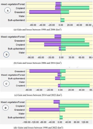
The gains and losses of the different land use categories in a Vea catchment over the 24-year period (1998–2022) are presented in Figure 6a–d. The LULCC is characterized by very contrasting changes in land use, with the green color representing gains per class in km2 and the wine color indicating losses in the land use category. Figure 6a shows Cropland and grassland increased about 62.4 and 18.01 km², respectively, between 1998 and 2006. While mixed vegetation/forest lost about 10.87 km², there were no losses in the water area and built-up area category. In the second period (2006–2014), cropland increased by 83.81 km², while grassland and mixed vegetation/forest lost −93.84 and 19.38 km², respectively (Figure 6b). A similar trend is observed in 2014–2022, where cropland increases by 55.17 km², while grassland and mixed vegetation/forests lose −58.16 and 5.04 km², respectively (Figure 6c). Figure 6d depicts that between 1998 and 2022, cropland and built-up area/bare land increase by 142.16 and 15.12 km², respectively, while grassland, mixed vegetation/forest and water are lost −147.36, −30.15 and −0.07 km², respectively. The study support the Losses in the Savannah forest are corroborated by Atulley et al. claim that the Savannah forest ecosystem is subject to many stresses leading to forest degradation; Extraction of firewood, uncontrolled bush fires, illegal mining and conversion of forests to cropland.

Figure 6. (a) Gain and losses between 1998 and 2006 (km2). (b) Gain and losses between 2006 and 2014 (km²). (c) Gain and losses between 2014 and 2022 (km2). (d) Gains and losses between 1998 and 2022 (km²).

3.6. Contributors to land use/land cover changes from 1998 to 2022

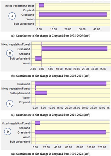
In order to observe the transformations of all other LULC classes to cropland, plots of contributors (LULC types transformed into other LULC types) on the dynamics of cropland area over the 24-year period, expressed in km2 were constructed (Figure 7a–d). The main contributor behind the expansion of cropland over the last 24 years was grassland, followed by mixed vegetation/forest. From 1998 to 2006, grassland contributed about 47 km², while mixed vegetation/forest contributed 3.4 km² to the increase in cropland. From 2006 to 2014, grassland contributed about 37 km², followed by mixed vegetation/forest which contributed 0.29 km². From 2014 to 2022, grassland contributed about 43 km², while built-up/bare land contributed about 7 km². Generally, from 1998 to 2022, grassland and forest/mixed vegetation were the main contributors to the increase in cropland in the Vea catchment and contributed about 127 and 8.5 km², respectively.

Figure 7. (a) Contributors to Net change in cropland from 1998 to 2006 (km2). (b) Contributors to Net change in Cropland from 2006 to 2014 (km2). (d) Contributors to Net change in Cropland from 2014 to 2022 (km²). (d) Contributors to Net change in Cropland from 1998 to 2022 (km²).

3.7. Potential LULC change drivers in the Vea catchment

The results of the relative importance index (RII) analysis showed that agricultural expansion (0.80), followed by firewood extraction (0.75) and charcoal production (0.68) were the leading drivers of the change in LULC (Table 9). As proximity drivers of LULC change function at the local community level, they directly reflect how and why local land cover changes and transforms.

The main underlying drivers of LULC change in the Vea catchment are unprecedented population growth (0.85) which are followed by land degradation (0.78), lack of livelihood options (0.72), lack of law enforcement (0.70) and dry spell (0.63) (Table 10).

Table 10. Identified potential land use/land cover drivers in Vea catchment.

No	Proximity drivers	RII	Rank	Underlying drivers	RII	Rank
1	Agricultural Expansion	0.80	2	Population growth	0.85	1
2	Firewood extraction	0.75	4	Land degradation	0.78	3
3	charcoal production	0.68	7	Lack law enforcement	0.70	6
4	Overgrazing	0.65	8	dry spell	0.63	10
5	Settlement	0.64	9	Lack of livelihood option	0.72	5
6	Bush fires	0.60	12	Land tenure	0.62	11

Understanding the patterns and drivers of LULC change is necessary for rational and specific planning of sustainable land management (Kamwi et al. 2018). Significant LULC changes (grassland decline, cropland, built-up/bare land expansion, and mixed vegetation/woodland decline) occurred in the study area due to various driving factors. Population growth appears to be the main driver of LULC change, most notably the expansion of cropland at the expense of grassland and mixed vegetation/forests. It confirms the results of Abebe et al. (2022) reported in Gubalafito district of northeastern Ethiopia and in Kuma et al. (2022) were carried out from the Bilat catchment in southern Ethiopia, according to which more than half of the studied basins were arable land. Population growth, lack of livelihood opportunities, inappropriate agricultural trends associated with land degradation, mono-cultural market culture that encourages farmers to acquire more arable land for higher yields, and institutional weakness in the implementation of land use policies have led to the increase in cropland.

3.8. Model validation

Comparisons between actual and simulated LULC 2022 maps were performed to validate the predicted maps. The validation results between the simulated and actual LULC test summary of the model are presented in Table 11. The accuracy of the prediction was confirmed by comparing the predicted LULC for 2022 with the classified LULC for the same year. The statistics show that Kno is 0.9016, Klocation is 0.9120, and K-standard, which is the overall kappa, is 0.9043. This means that the simulation is perfectly capable of pinpointing the location and also the quantity. Therefore, there is very little quantification and location error and all K-index values exceed the minimum acceptable standard of 82% (Mishra et al. 2014). In this study, all values of Kappa indices are greater than 95%, meaning that the agreement between the predicted and the actual map of 2022 is relatively high, showing a strong projection ability of the model to utilize it for LULC change prediction in 2038 and 2054 (Table 11). LULC prediction of the landscape of the current study is based on the change of driver effects. Four spatial factors such as distance to road, river, slope and elevation were used (Table 12). River, slope, and height data were obtained from open topography with a resolution of 30 * 30 m.

Table 11. The k-index values of the simulated LULC map of 2022.

Index	Value
K no	0.9016
K Location	0.9120
K standard	0.9043

Table 12. Driver factors and their weight.

No	Factors (spatial drivers)	Weight (%)
1	Distance to roads	0.24
2	Distance to rivers	0.24
3	Elevation	0.18
4	Slope	0.18

The visual comparison between the actual LULC 2022 map and the simulated map (Figure 8) is relatively similar. The common area of all land use types from the actual and simulated maps also shows an acceptable decision range, where the difference in actual area between the simulated map and the 2022 reality for all LULC types is less than 5% (Table 13). Regardless of the magnitude of variability among the classified land-use types, the best agreement of change trends was observed with past LULC changes and predicted LULC change outcomes (Tables 3, 13). The high degree of consistency between the actual and predicted spatial land use distribution confirms that the developed CA-Markov model is best suited for predicting changes in the LULC of the Vea catchment in 2038 and 2054.

Figure 8. Simulated and actual LULC maps of 2022.

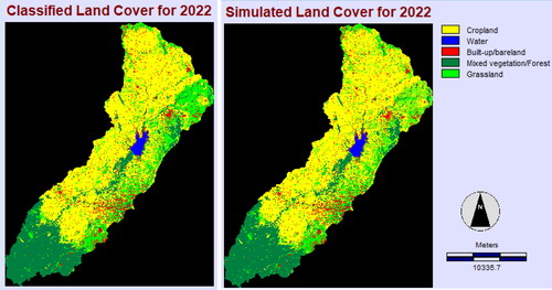
Table 13. LULC area coverage, and rate of changes between 2022 and 2054.

LULC classes	Area of 2022		Area of 2038		Area of 2054		Gain/loss 2022–2054 (%)
	km^2	%	km^2	%	km^2	%	Km^2	%	Annual change (%)
Cropland	174.5	52.87	179	54.24	182	55.15	7.5	4.3	0.13
Water	3.41	1.03	3.1	0.94	3	0.91	−0.41	−12.02	−0.37
Built-up/bare land	22.3	6.75	24	7.3	25.2	7.64	2.9	13.01	0.45
Mixed v/forest	75.2	22.7	72	21.8	70	21.2	−5.2	−7.1	−0.22
Grassland	54.9	16.6	52.1	15.8	50	15.2	−4.9	−8.9	−0.31

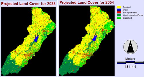
3.9. Prediction of LULC changes

The predicted land use/land cover types for 2038 and 2054 were calculated using the CA Markov model and are plotted in areal in Table 13. The area of grassland and mixed vegetation/forest decreased from 54.9 km² in 2022 to 52 km² in 2038 and 72 km² in 2022 to 72 km² in 2054. From 2038 (179 km²) to 2054 (182 km²) and from 2038 (24 km²) to 2054 (25.2 km²) there will be a continuous increase in cropland and built-up/bare land. On the other hand, the amount of water will decrease from 2038 (3.1 km²) to 2054 (3 km²). The expansion of cropland and built-up/bare land is expected to increase at the expense of mixed vegetation/forest and grassland. Over 2022–2054 grassland and mixed v./forest would have exhibited the highest loss by 4.9 km², and 5.2 ha, respectively (Table 13). The lowest loss could be scored by water body. While the highest gain would be observed in cropland (Figure 9).

Figure 9. The predicted 2038 and 2054 LULC of the Vea catchment.

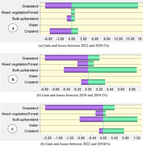
3.10. Predicted LULC category gains and losses from 2022 to 2054

The gains and losses of the different land use categories in the Vea catchment over the 32-year period (2022–2054) are shown in Figure 10a–d. The LULC change is characterized by very contrasting changes in land use, with the green color representing gains per class in percent and the wine color indicating losses in the land use category. Figure 10a shows that, in the period 2022–2038 cropland increased by 2%, while grassland and mixed vegetation/forest lost −7 and 0.68%, respectively. These dynamics reflect the saturation of cropland caused by significant demographic developments over the past 20 years. A similar trend is predicted in 2038–2054, where cropland increases by 3%, while grassland and mixed vegetation/forests lose −0.80 and −2%, respectively (Figure 10b). In general, between 2022 and 2054, cropland and built-up area/bare land increased by 0.8 and 1.2%, respectively, while grassland, mixed vegetation/forest, and water are −2, −0.3 and −0.02 km², respectively, lost (Figure 10c). This finding confirms the Losses in the Savannah forest are corroborated by Atulley et al. claim that the Savannah forest ecosystem is subject to many stresses leading to forest degradation; Extraction of firewood, uncontrolled bush fires, illegal mining and conversion of forests to cropland.

Figure 10. (a) Gain and losses between 2022 and 2038 (%). (b) Gain and losses between 2038 and 2054 (%). (c) Gain and losses between 2022 and 2054 (%).

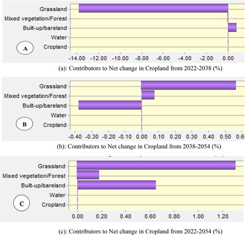
3.11. Contributors to predicted land use/land cover changes from 2022 to 2054

In order to observe the conversions of all other LULC classes into cropland, plots of the contributors (LULC types converted into other LULC types) on the dynamics of cropland area over the period of 32 years, expressed in %, are presented in Figure 11. The main factor behind the expansion of cropland over the last 32 years was grassland, followed by mixed vegetation/forest. From 2022 to 2038, Built-up/bare land contributed about 0.5% to the increase in cropland. From 2038 to 2054, grassland contributed about 0.58%, while mixed vegetation/forest contributed about 0.1% and built up is −0.4%. In general, from 2022 to 2054, grassland, built-up/bare land, and forest/mixed vegetation were the main drivers for the increase in cropland in the Vea catchment, contributing about 1.5, 0.7 and 0.2%, respectively.

Figure 11. (a) Contributors to net change in cropland from 2022 to 2038 (%). (b) Contributors to net change in Cropland from 2038 to 2054 (%). (c) Contributors to net change in Cropland from 2022 to 2054 (%).

3.12. LULC change impact on water availability for irrigation

Most countries in sub-Saharan Africa (SSA) are vulnerable to LULC changes (Iannella et al. 2021). The LULC change puts increasing stress on future water. The gradual degradation of water bodies can lead to degradation of landscape components (flora, soil and fauna), leading to desertification, which in turn leads to health problems, poverty and loss of biodiversity (Kelly et al. 2015). Deforestation is one of the alterations in LULC, which is believed to be the primary source of variations in hydrological processes such as surface runoff, sediment production, evapotranspiration, groundwater, infiltration, lateral flow and rainfall interception (Getachew and Manjunatha 2022). Changes in the LULC will be driven by human interaction, which in turn will produce changes that alter the availability of water resources (Daba and You 2022). The Vea catchment is home to one of the two major irrigation systems in the Upper East Region of Ghana (Limantol et al. 2016). Land use and climate change are the two main driving forces affecting the hydrological systems of the Vea catchment. The availability of future water for irrigation is highly dependent on land use planning and management in an ever-changing environment. On the other hand, ongoing human behavior continues to transform LULC to meet increased demand, particularly due to significant population growth and agricultural expansion.

The Vea catchment has high precipitation variability and high temperatures, and relatively high surface water evaporation. This leads to a low water level in the catchment area. Therefore, high evapotranspiration leads to a reduction in base flow and groundwater, resulting in a reduction in water production and runoff. Decreased water production can lead to water scarcity and extreme concern about water supplies. Assessing water availability in the catchment requires a LULC change assessment to study the ecological and hydrological conditions for future viable water resource management. Several studies have examined the impact of LULC on water resources in many countries around the world. For example, in eastern and southern Africa, changes in LULC are the main reason for reducing river flow and surface runoff (Namugize et al. 2018), leading to water shortages. Changes in the LULC not only affect water availability for irrigation but also affect the quality of water resources through various mechanisms. Changes in the LULC, such as fragmentation and degradation of the land landscape, adversely affect water quality in the catchment by moving sediments and chemicals into the reservoir. In addition, water pollution is common with rapid changes in land use and land cover, particularly from the emission of greenhouse gases such as methane and CO₂ released by deforestation and rice production in the Vea catchment. This study has shown that there is a positive association between LULC changes and water availability for irrigation, suggesting that LULC changes contribute to water scarcity. Due to the projected changes in LULC in the Vea catchment, the water is expected to continue to be impacted. Therefore, appropriate measures must be taken to reduce the impact of LULC changes on water availability, especially for irrigation, as the area has high evapotranspiration, which is greater than rainfall.

4. Conclusion

In order to develop future policies and strategies for river basin management, it is necessary to know the dynamics of changes in natural resources and evaluate future scenarios. Using the CA-Markov model, this study simulated future land use patterns for 2038 and 2054 for the Vea catchment. The prediction simulations were performed at Terrset based on historical land use maps from 1998, 2006, 2014 and 2022. To validate the model, the projected LULC map for 2022 was compared to the actual map for 2022 and after successful validation, the LULC map for 2038 and 2054 was stimulated. The results of the model validation demonstrated the LCM's ability to predict the future LULC state of the study area with an accuracy of over 82% of the minimum acceptable level of accuracy. Overall, the LULC maps between 1998 and 2022 are characterized by large increases in the cropland category and significant losses in grassland and mixed vegetation/forest. Cropland is expected to increase to 182 km² by 2054, while grassland and mixed vegetation/forest area will decrease to 50 and 70 km², respectively, in 2054. The change maps show that the loss of grassland and varied vegetation/forest is due to cropland expansion. Future LULC maps show a continued increase in cropland and built-up areas at the expense of grassland, water and mixed vegetation/forest cover. As indicated by the majority of respondents, the increase in cropland could be related to the growing population and the associated demand for food security. The significant conversion of grassland and mixed vegetation/forest to cropland around the Vea catchment is a cause for concern about water availability for irrigation because this will increase sedimentation and endanger storage in the reservoir. This study found a positive relationship between LULC changes and irrigation water availability, implying that LULC changes contribute to water scarcity in the study catchment since it affects the storage of the reservoir. This study’s findings are encouraging for Upper East Ghana, where information on historical, current, and future patterns of LULC is critical for water availability for agriculture in the face of climate change. To promote sustainable growth and decrease the intensity of changes around the reservoir, policymakers must adopt timely management activities. It is believed that the findings of this study will provide an important foundation for planning the long-term management of forest water resources in the Vea catchment.

Authors’ Contributions

Gemechu Fufa Arfasa, conceptualization, data collection, analysis, writing of the draft manuscript, and editing; Prof. Ebenezer Owusu Sekyere and Dzigbodi Adzo Doke gave guidance for the paper, reviewing, commenting, and editing. All authors read and approved the final manuscript.

Ethical approval

No parts of the study that concern about human and/or animal lab in this study.

Acknowledgements

The authors duly acknowledge the Material support from the West Africa Centre for Water, Irrigation and Sustainable Agriculture (WACWISA), an African Center of Excellence under the auspices of the World Bank and the Government of Ghana. We, the authors are pleased to thank the USGS for the provision of Landsat data. We are also grateful to the sampled respondents who provided us with the required information. The Authors are grateful to Dr. Joan Atulley for her guidance on the application of Terrset software for data analysis. The authors are grateful to all the anonymous reviewers whose invaluable suggestions improved the quality of this manuscript.

Disclosure statement

The authors declare that they have no competing interests.

Data availability statement

The data that has been used is confidential. All Landsat images were acquired from the United States Geological Survey (USGS) website available at (https://earthexplorer.usgs.gov).

Additional information

Funding

No special fund for this study.

References

- Larbi I, Forkuor G, Hountondji FCC, Agyare WA, Mama D. 2019. Predictive land use change under business-as-usual and afforestation scenarios in the Vea Catchment, West Africa. IJARSG. 8(1):3011–3029. doi:10.23953/cloud.ijarsg.416.
- Abebe G, Getachew D, Ewunetu A. 2022. Analysing land use/land cover changes and its dynamics using remote sensing and GIS in Gubalafito district, Northeastern Ethiopia. SN Appl Sci. 4(1):30. doi:10.1007/s42452-021-04915-8.
- Abbas Z, Jaber HS. 2020. Accuracy assessment of supervised classification methods for extraction land use maps using remote sensing and GIS techniques. IOP Conf Ser: Mater Sci Eng. 745(1):012166. doi:10.1088/1757-899X/745/1/012166.
- Abdurahman A, Yirsaw E, Nigussie W, Hundera K. 2023. Past and future land-use/land-cover change trends and its potential drivers in Koore’s agricultural landscape, Southern Ethiopia. Geocarto Int. 38(1):1–25. doi:10.1080/10106049.2023.2229952.
- Aburas MM, Ho YM, Ramli MF, Ash’aari ZH. 2016. The simulation and prediction of spatio-temporal urban growth trends using cellular automata models: a review. Int J Appl Earth Obs Geoinf. 52:380–389. doi:10.1016/j.jag.2016.07.007.
- Brown JF, Tollerud HJ, Barber CP, Zhou Q, Dwyer JL, Vogelmann JE, Loveland TR, Woodcock CE, Stehman SV, Zhu Z, et al. 2020. Lessons learned implementing an operational continuous United States national land change monitoring capability: the Land Change Monitoring, Assessment, and Projection (LCMAP) approach. Remote Sens Environ. 238:111356. doi:10.1016/j.rse.2019.111356.
- Chang Y, Hou K, Li X, Zhang Y, Chen P. 2018. Review of land use and land cover change research progress. IOP Conf Ser: earth Environ Sci. 113:012087. doi:10.1088/1755-1315/113/1/012087.
- Chisanga CB, Shepande CC, Nkonde E. 2022. CA-Markov approach in dynamic modelling of LULCC using ESA CCI products over Zambia. In Geographic information systems and applications in coastal studies. London: IntechOpen.
- Daba MH, You S. 2022. Quantitatively assessing the future land-use/land-cover changes and their driving factors in the upper stream of the Awash River based on the CA–Markov model and their implications for water resources management. Sustainability. 14(3):1538. doi:10.3390/su14031538.
- Eastman JR, Toledano J. 2018. A short presentation of the land change modeler (LCM). In: Camacho Olmedo M, Paegelow M, Mas JF, et al., Editors. Geomatic approaches for modeling land change scenarios; p. 499–505.
- FAO. 2011. The state of the world’s land and water resources for food and agriculture managing systems at risk. Rome: Food and Agriculture Organization of the United Nations.
- FAO. 2020. Global forest assessment resources 2020 (No.163). Rome, Italy: Forestry Paper.
- Foody GM. 2020. Explaining the unsuitability of the kappa coefficient in the assessment and comparison of the accuracy of thematic maps obtained by image classification. Remote Sens Environ. 239:111630. doi:10.1016/j.rse.2019.111630.
- Friedenthal J, Maxwell SM, Munné S, Kramer Y, McCulloh DH, McCaffrey C, Grifo JA. 2018. Next generation sequencing for preimplantation genetic screening improves pregnancy outcomes compared with array comparative genomic hybridization in single thawed euploid embryo transfer cycles. Fertil Steril. 109(4):627–632. doi:10.1016/j.fertnstert.2017.12.017.
- Gashaw T, Tulu T, Argaw M, Worqlul AW. 2017. Evaluation and prediction of land use/land cover changes in the Andassa watershed, Blue Nile Basin, Ethiopia. Environ Syst Res. 6(1):1–15. doi:10.1186/s40068-016-0078-x.
- Getachew B, Manjunatha BR. 2022. Impacts of land‐use change on the hydrology of Lake Tana Basin, Upper Blue Nile River Basin, Ethiopia. Glob Chall. 6(8):2200041. doi:10.1002/gch2.202200041.
- Gharaibeh A, Shaamala A, Obeidat R, Al-Kofahi S. 2020. Improving land-use change modeling by integrating ANN with Cellular Automata-Markov Chain model. Heliyon. 6(9):e05092. doi:10.1016/j.heliyon.2020.e05092.
- Govender T, Dube T, Shoko C. 2022. Remote sensing of land use-land cover change and climate variability on hydrological processes in Sub-Saharan Africa: key scientific strides and challenges. Geocarto Int. 37(25):10925–10949. doi:10.1080/10106049.2022.2043451.
- Hamad R, Balzter H, Kolo K. 2018. Predicting land use/land cover changes using a CA-Markov model under two different scenarios. Sustainability. 10(10):3421. doi:10.3390/su10103421.
- Han H, Yang C, Song J. 2015. Scenario simulation and the prediction of land use and land cover change in Beijing, China. Sustainability. 7(4):4260–4279. doi:10.3390/su7044260.
- Hansen RE. 2022. Change detection on shipwrecks using synthetic aperture sonar–North Sea Wrecks Task 3.5 Deep Water Case Study.
- Hoque M, Cui S, Islam I, Xu L, Ding S. 2021. Dynamics of plantation forest development and ecosystem carbon storage change in coastal Bangladesh. Ecol Indic. 130:107954. doi:10.1016/j.ecolind.2021.107954.
- Hua A. 2017a. Application of Ca-Markov model and land use/land cover changes in Malacca River Watershed, Malaysia. Appl Ecol Env Res. 15(4):605–622. doi:10.15666/aeer/1504_605622.
- Hua AK. 2017b. Land use land cover changes in detection of water quality: a study based on remote sensing and multivariate statistics. J Environ Public Health. 2017:7515130. doi:10.1155/2017/7515130.
- Iannella M, De Simone W, D'Alessandro P, Biondi M. 2021. Climate change favours connectivity between virus-bearing pest and rice cultivations in sub-Saharan Africa, depressing local economies. PeerJ. 9:e12387. doi:10.7717/peerj.12387.
- Kafy, A. A., Raikwar, V., Rakib, A. A., Kona, M. A., Ferdousi, J. (2021). Geospatial approach for developing an integrated water resource management plan in Rajshahi, Bangladesh. Environ Chall. 4, 100139. doi:10.1016/j.envc.2021.100139.
- Kamwi JM, Cho MA, Kaetsch C, Manda SO, Graz FP, Chirwa PW. 2018. Assessing the spatial drivers of land use and land cover change in the protected and communal areas of the Zambezi Region, Namibia. Land. 7(4):131. doi:10.3390/land7040131.
- Kelly C, Ferrara A, Wilson GA, Ripullone F, Nolè A, Harmer N, Salvati L. 2015. Community resilience and land degradation in forest and shrubland socio-ecological systems: evidence from Gorgoglione, Basilicata, Italy. Land Use Policy. 46:11–20. doi:10.1016/j.landusepol.2015.01.026.
- Khawaldah H, Farhan I, Alzboun N. 2020. Simulation and prediction of land use and land cover change using GIS, remote sensing and CA-Markov model. Global J Environ Sci Manag. 6(2):215–232.
- Kuma HG, Feyessa FF, Demissie TA. 2022. Landuse/land-cover changes and implications in Southern Ethiopia: evidence from remote sensing and informants. Heliyon. 8(3):e09071. doi:10.1016/j.heliyon.2022.e09071.
- Leta MK, Demissie TA, Tränckner J. 2021. Modeling and prediction of land use land cover change dynamics based on land change modeler (Lcm) in nashe watershed, upper blue Nile Basin, Ethiopia. Sustainability. 13(7):3740. doi:10.3390/su13073740.
- Limantol AM, Keith BE, Azabre BA, Lennartz B. 2016. Farmers’ perception and adaptation practice to climate variability and change: a case study of the Vea catchment in Ghana. Springerplus. 5(1):830. doi:10.1186/s40064-016-2433-9.
- Lu D, Li G, Moran E. 2014. Current situation and needs of change detection techniques. Int J Image Data Fusion. 5(1):13–38. doi:10.1080/19479832.2013.868372.
- Mahamud M, Samat N, Tan M, Chan N, Tew Y. 2019. Prediction of future land use land cover changes of Kelantan, Malaysia. International Archives of the Photogrammetry, Remote Sensing & Spatial Information Sciences
- Mahmoud SH, Alazba A. 2016. Land cover change dynamics mapping and predictions using EO data and a GIS-cellular automata model: the case of Al-Baha region, Kingdom of Saudi Arabia. Arab J Geosci. 9(5):1–20. doi:10.1007/s12517-016-2439-1.
- Megahed Y, Cabral P, Silva J, Caetano M. 2015. Land cover mapping analysis and urban growth modelling using remote sensing techniques in Greater Cairo Region—Egypt. IJGI. 4(3):1750–1769. doi:10.3390/ijgi4031750.
- Mishra K, Boynton L, Mishra A. 2014. Driving employee engagement: the expanded role of internal communications. Int J Bus Commun. 51(2):183–202. doi:10.1177/2329488414525399.
- Mohajane M, Essahlaoui A, Oudija F, Hafyani ME, Hmaidi AE, Ouali AE, Randazzo G, Teodoro AC. 2018. Land use/land cover (LULC) using landsat data series (MSS, TM, ETM + and OLI) in Azrou Forest, in the Central Middle Atlas of Morocco. Environments. 5(12):131. doi:10.3390/environments5120131.
- Muhammad R, Zhang W, Abbas Z, Guo F, Gwiazdzinski L. 2022. Spatiotemporal change analysis and prediction of future land use and land cover changes using QGIS MOLUSCE plugin and remote sensing big data: a case study of Linyi, China. Land. 11(3):419. doi:10.3390/land11030419.
- Munthali M, Mustak S, Adeola A, Botai J, Singh S, Davis N. 2020. Modelling land use and land cover dynamics of Dedza district of Malawi using hybrid Cellular Automata and Markov model. Remote Sens Appl: Soc Environ. 17:100276. doi:10.1016/j.rsase.2019.100276.
- Nadoushan MA, Soffianian A, Alebrahim A. 2015. Modeling land use/cover changes by the combination of Markov chain and cellular automata Markov (CA-Markov) models. J Earth Environ Health Sci. 1(1):16. doi:10.4103/2423-7752.159922.
- Nageswaran S, Arunkumar G, Bisht AK, Mewada S, Kumar J, Jawarneh M, Asenso E. 2022. Lung cancer classification and prediction using machine learning and image processing. Biomed Res Int. 2022:1755460. doi:10.1155/2022/1755460.
- Namugize JN, Jewitt G, Graham M. 2018. Effects of land use and land cover changes on water quality in the uMngeni river catchment, South Africa. Phys Chem Earth Parts a/b/c. 105:247–264. doi:10.1016/j.pce.2018.03.013.
- Nath V, Chattopadhyay C, Desai KA. 2023. NSLNet: an improved deep learning model for steel surface defect classification utilizing small training datasets. Manuf Lett. 35:39–42. doi:10.1016/j.mfglet.2022.10.001.
- Olmedo MTC, Pontius RG, Jr, Paegelow M, Mas J-F. 2015. Comparison of simulation models in terms of quantity and allocation of land change. Environ Modell Softw. 69:214–221. doi:10.1016/j.envsoft.2015.03.003.
- Pérez-Vega A, Mas JF, Ligmann-Zielinska A. 2012. Comparing two approaches to land use/cover change modeling and their implications for the assessment of biodiversity loss in a deciduous tropical forest. Environ Model Softw. 29(1):11–23. doi:10.1016/j.envsoft.2011.09.011.
- Qasim M, Hubacek K, Termansen M, Fleskens L. 2013. Modelling land use change across elevation gradients in district Swat, Pakistan. Reg Environ Change. 13(3):567–581. doi:10.1007/s10113-012-0395-1.
- Roy DP, Wulder MA, Loveland TR, Woodcock CE, Allen RG, Anderson MC, Helder D, Irons JR, Johnson DM, Kennedy R, et al. 2014. Landsat-8: science and product vision for terrestrial global change research. Remote Sens Environ. 145:154–172. doi:10.1016/j.rse.2014.02.001.
- Rwanga SS, Ndambuki JM. 2017. Accuracy assessment of land use/land cover classification using remote sensing and GIS. IJG. 08(04):611–622. doi:10.4236/ijg.2017.84033.
- Shawul AA, Chakma S. 2019. Spatiotemporal detection of land use/land cover change in the large basin using integrated approaches of remote sensing and GIS in the Upper Awash basin, Ethiopia. Environ Earth Sci. 78(5):141. doi:10.1007/s12665-019-8154-y.
- Sleeter BM, Sohl TL, Loveland TR, Auch RF, Acevedo W, Drummond MA, Sayler KL, Stehman SV. 2013. Land-cover change in the conterminous United States from 1973 to 2000. Global Environ Change. 23(4):733–748. doi:10.1016/j.gloenvcha.2013.03.006.
- Springgay E, Casallas Ramirez S, Janzen S, Vannozzi Brito V. 2019. The forest–water nexus: an international perspective. Forests, 10(10), 915. doi:10.3390/f10100915.
- Vázquez-Quintero G, Solís-Moreno R, Pompa-García M, Villarreal-Guerrero F, Pinedo-Alvarez C, Pinedo-Alvarez A. 2016. Detection and projection of forest changes by using the Markov Chain Model and cellular automata. Sustainability. 8(3):236. doi:10.3390/su8030236.
- Visa S, Ramsay B, Ralescu AL, Van Der Knaap E. 2011. Confusion matrix-based feature selection. Maics. 710(1):120–127.
- Wu K-y, Zhang H. 2012. Land use dynamics, built-up land expansion patterns, and driving forces analysis of the fast-growing Hangzhou metropolitan area, eastern China (1978–2008). Appl Geogr. 34:137–145. doi:10.1016/j.apgeog.2011.11.006.
- Xie C, Batty M, Zhao K. 2007. Simulating emergent urban form using agent-based modeling: Desakota in the Suzhou-Wuxian region in China. Ann. Assoc. Am. Geogr. 97(3):477–495. doi:10.1111/j.1467-8306.2007.00559.x.
- Xing H, Meng Y, Shi Y. 2018. A dynamic human activity‐driven model for mixed land use evaluation using social media data. Trans GIS. 22(5):1130–1151. doi:10.1111/tgis.12447.
- Yirsaw E, Wu W, Shi X, Temesgen H, Bekele B. 2017. Land use/land cover change modeling and the prediction of subsequent changes in ecosystem service values in a coastal area of China, the Su-Xi-Chang Region. Sustainability. 9(7):1204. doi:10.3390/su9071204.
- Zhang CL, Zhang TJ, Guo YN, Yang LQ, He MW, Shi JZ, Ni JX. 2008. Effect of neurolytic celiac plexus block guided by computerized tomography on pancreatic cancer pain. Dig Dis Sci. 53(3):856–860. doi:10.1007/s10620-007-9905-2.
- Zhou X, Chen H. 2018. Impact of urbanization-related land use land cover changes and urban morphology changes on the urban heat island phenomenon. Sci Total Environ. 635:1467–1476. doi:10.1016/j.scitotenv.2018.04.091.