Landslide susceptibility mapping with feature fusion transformer and machine learning classifiers incorporating displacement velocity along Karakoram highway

Abstract

The Karakoram Highway (KKH) is a pivotal gateway within the framework of the China-Pakistan Economic Corridor. Nevertheless, its distinct and intricate geographical characteristics make it susceptible to recurrent landslides. As an essential tool, landslide susceptibility mapping (LSM) is significant in managing and alleviating landslides near the KKH. Moreover, landslide conditioning factors (LCFs) are crucial determinants influencing the outcomes of LSM. However, existing methods primarily rely on machine learning algorithms, which do not adequately account for the intricate spatial characteristics and patterns between LCFs and landslide occurrences. In response, this study introduces the feature fusion transformer (FFTR) module, constructed based on the foundations of the transformer framework, to fuse the spatial information features of all LCFs. Subsequently, the abstract high-level spatial features obtained are fed into diverse machine learning classifiers, including random forest (RF), extreme gradient boosting (XGBoost), gradient boosting decision trees (GBDT), categorical boosting (CatBoost), and extremely randomized trees (ET), to generate landslide susceptibility maps. Displacement velocity calculated by Persistent Scatterer Interferometric Synthetic Aperture Radar (PSInSAR) is incorporated in the LSM. The results demonstrate that FFTR-RF achieves premium performance in the area under the curve (AUC) (94%), accuracy (87.31%), precision (87.21%), recall (88.02%), and F₁-score (87.61%). Incorporating displacement velocity into LSM results predicted by models enhances the comprehensiveness of LSM. These methods will furnish early warning systems for landslide disasters along the KKH, thus aiding recommendations for mitigating landslides’ social and economic losses.

Keywords:

• Feature fusion transformer
• random forest
• landslide susceptibility mapping
• Karakoram highway
• displacement velocity

1. Introduction

China-Pakistan Economic Corridor (CPEC) is a paradigmatic project and flagship initiative of China’s ambitious ‘Belt and Road’ initiative (Abid and Ashfaq 2015; Javaid 2016; Khan and Liu 2019). As a critical strategic route, the KKH is often called the ‘Friendship Road’ between China and Pakistan (Nilofar et al. 2014). It has catalyzed economic and trade cooperation between China and Pakistan (Kulsoom et al. 2023). The KKH faces significant challenges due to its high-altitude mountainous terrain, intricate geographical conditions, and intense precipitation, making it highly susceptible to landslides (Hussain et al. 2023). These landslides often destroy bridges and road blockages and cause casualties and significant socio-economic losses (Zimmerman 2015; Ali et al. 2019). Furthermore, landslides exhibit complex causative characteristics, necessitating careful consideration of various conditioning factors when creating susceptibility maps for landslide-prone areas (Wang et al. 2019).

LSM aims to calculate the likelihood of occurrence of landslides within a specific area based on the landslide conditioning factors (LCFs) (Brabb 1985; Guzzetti et al. 1999). LSM techniques can be classified into statistical, empirical, physics-based, and machine-learning approaches (Guzzetti et al. 2012; Dou et al. 2019; Whiteley et al. 2019; Hussain et al. 2022). However, the development of statistical, empirical, and physics-based methods has encountered limitations (Huang et al. 2018; Roy et al. 2019; Di Napoli et al. 2020; Huang et al. 2020a; Merghadi et al. 2020; Loche et al. 2022). In recent years, machine learning methods have shown higher accuracy and efficiency in LSM, as they can capture non-linear relationships between LCFs and landslide data (Melchiorre et al. 2006; Merghadi et al. 2020; Qing et al. 2020). Various machine learning algorithms have been employed in this context, including but not limited to logistic regression, support vector machine, RF, XGBoost, naive Bayes, and CatBoost (Huang and Zhao 2018; Hussain et al. 2021; Khalil et al. 2022; Li et al. 2022; Ye et al. 2022; Zhang et al. 2022; Gupta and Shukla 2023; Huang et al. 2023a). However, there is still room for development in LSM based on the above research. The results of LSM significantly rely on the distribution characteristics of LCFs. Therefore, considering contextual features in geographic spatial information is crucial for LSM. Nevertheless, traditional machine learning methods struggle to adequately account for the complex contextual spatial information and patterns among landslide data and various LCFs (Chen et al. 2021). Therefore, it is imperative to extend the research on LSM into deep learning to enrich the comprehension of the spatial relationship between landslides and LCFs and uncover intricate patterns of landslide occurrences in space.

As deep learning rapidly advances, researchers have focused on incorporating deep learning methods into LSM to understand and represent regions prone to landslides (Bui et al. 2020; Huang et al. 2020b). Several deep learning techniques including the convolutional neural network (CNN), residual network (ResNet), recurrent neural network (RNN), and long short-term memory (LSTM), have been successfully employed in LSM (Wang et al. 2019; Fang et al. 2020; Wang et al. 2020; Chen et al. 2021; Ngo et al. 2021; Lv et al. 2022; Huang et al. 2023b; Jiang et al. 2023; Zhang et al. 2023). In recent years, the development of transformer architecture has shown remarkable success in various downstream tasks (Zheng et al. 2021; Amatriain 2023). The effectiveness of the transformer stems from its self-attention mechanism (Yang et al. 2021). It is precisely due to its remarkable ability to unearth spatial relationships that the transformer can learn the patterns and features of landslide occurrences in space, enabling a comprehensive analysis of large-scale landslide susceptibility. The multi-head attention mechanism further enriches feature representations and explores intricate relationships between different features (Vaswani et al. 2017). Therefore, the transformer holds significant advantages in capturing long-range contextual spatial relationships between landslide data and various LCFs. Utilizing the transformer to fuse multiple complex LCF features demonstrates the capacity to improve LSM. Nonetheless, it is worth noting that dynamic surface displacement is a crucial dataset capable of capturing landslide susceptibility but is often disregarded in the mapping process based on deep learning models.

Hence, incorporating displacement velocity into the LSM is necessary. Surface displacement velocity effectively reflects the dynamic changes in slopes. Therefore, recent studies have detected and updated landslide inventories based on surface displacement velocity (Zhao et al. 2018; Rehman et al. 2020; Su et al. 2021; Su et al. 2022; Hussain et al. 2023). InSAR is a new earth observation technique, notable for its extensive monitoring time and the capacity to calculate precise and reliable data regarding surface deformation (Mondini et al. 2021). Among InSAR techniques, PS-InSAR is an advanced InSAR technique well-suited for the millimeter-level monitoring of large-scale surface deformation (Beladam et al. 2019). The timely acquisition of slope displacement velocity is attainable through the PS-InSAR technique, and incorporating it into LSM is a viable option (Hussain et al. 2021). Subsequently, upon the computation of displacement velocity, its incorporation into LSM exhibits the potential for augmenting the overall reliability and comprehensiveness of the mapping.

Upon the preceding context, this study focuses on the buffer zone along the KKH as the study area and conducts LSM by considering fifteen LCFs that include topography, geology, hydrology, and others. The LCFs are categorized into continuous and discrete types and then fed into the FFTR module for feature fusion, resulting in the advanced spatial feature. Subsequently, the fused feature is input for various classifiers to compute landslide classification results within the region, including RF, XGBoost, GBDT, CatBoost, and ET classifiers. These results are further utilized to produce landslide susceptibility maps. Finally, the displacement velocity calculated through PS-InSAR is incorporated into the LSM to create the ultimate landslide susceptibility map. By generating the susceptibility maps, this study aims to contribute to the prevention and mitigation of life and property losses along the KKH and promote the development of the regions adjacent to the highway.

2. Methods

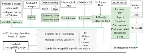
In summary, based on the source data shown in Figure 1, landslide inventory and LCFs were created. Firstly, all LCFs were input into landslide susceptibility prediction models to obtain susceptibility maps. Secondly, displacement velocity was calculated using the PSInSAR technique based on the Sentinel-1 datasets. Finally, the displacement velocity was integrated into the susceptibility maps predicted by the models, resulting in the generation of the final landslide susceptibility maps (Figure 1).

Figure 1. Flow chart of the study.

2.1. Study area

This study focuses on the KKH within the CPEC, which spans approximately 353 km in a northwest-southeast direction, with a 10 km buffer zone along the highway. The China-Pakistan Economic Corridor stretches from Kashgar in the north to Gwadar Port in the south, bordered by Tajikistan and Afghanistan to the east and China and India to the west (Figure 2). The region possesses a strategically significant geographical location.

Figure 2. Study area.

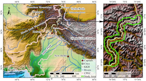
The corridor’s traverses multiple high-altitude mountain ranges, including the Tian Shan, Pamir, Karakoram, and Himalayan ranges (Searle et al. 1999). The corridor is adjacent to the Taklamakan Desert, the Tarim Basin, and the Qinghai-Tibet Plateau, encompassing parts of the Indian plains (Figure 2). The KKH, with its lowest point at 460 m and the highest point at 4,733 m, crosses numerous rivers and glaciers and experiences an annual rainfall ranging from 150 mm to 2,000 mm (Rashid et al. 2020). The region’s extremely high temperatures and heavy rainfall contribute to frequent landslides along the KKH (Yang et al. 2020). Due to its unique and treacherous geographical setting, the KKH is susceptible to frequent landslides.

2.2. Landslide inventory and conditioning factors

The landslide inventory is critically vital in documenting the occurrence and characteristics of landslides, including the locations and extents. It serves as a crucial basis for conducting LSM, enabling us to enhance the accuracy and reliability of methodologies (Guzzetti et al. 2012).

A comprehensive landslide inventory within the study area is developed, encompassing 547 individual landslide areas with a cumulative area of 245 km² (Figure 3). These areas include various landslides, such as debris flows, scree slopes, and rockfalls. Initially, relevant landslide disaster data from publications by the Geological Survey of Pakistan (GSP) represent authentic instances of landslide disasters within the study region, providing valuable data for analysis (Fayaz et al. 1985; Khan et al. 1986; Khan et al. 2003). Furthermore, the publication related to CPEC is also referenced (Yixuetao and Shao 2021). Moreover, Sentinel-2 satellite imagery (2022) combined with Google Earth imagery facilitated detailed observations and validation of the collected data, ensuring the landslide inventory’s reliability and robustness. Random sampling was conducted within the landslide areas to consider the spatial information of these landslides (Figure 3). Thus, there are 2,111 landslide locations and 2,145 non-landslide locations. These locations were randomly split into training and testing data with a ratio of 7:3 (Table 1).

Figure 3. Landslide areas.

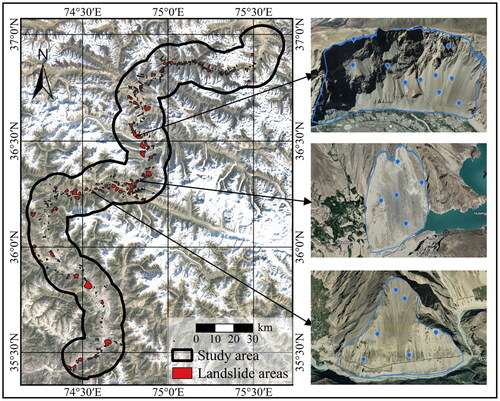
Table 1. Training and testing data.

Location type	Training data	Testing data
Landslide	1,460	651
Non-landslide	1,519	626

Due to the complex and multifaceted nature of landslide occurrences, which are influenced by various interacting factors, selecting conditioning factors is of utmost importance (Huang and Zhao 2018; Gaidzik and Ramírez-Herrera 2021). Therefore, considering the complex geographical environment and unique geological characteristics of the KKH, this study incorporates several conditioning factors to assess landslide hazards comprehensively.

The chosen conditioning factors include geology, which encompasses lithology (Table 2, Figure 7) and fault lines; topography, which includes elevation, curvature, plan curvature, profile curvature, aspect, slope, roughness, and topographic wetness index (TWI); hydrology, which encompasses distance to river and precipitation, as well as landcover, normalized difference vegetation Index (NDVI), and distance to road (Table 2, Figures 4–6). Among these, the influences of the river and road factors on landslide hazards are analyzed using Euclidean distance analysis, providing insights into the spatial relationships between these factors and landslide occurrences (El Jazouli et al. 2019). The calculation of NDVI utilized Sentinel-2 satellite imagery from May, July, and September 2022, coinciding with the surface deformation monitoring period. The calculation formula is as follows: (1) $$\mathit{NDVI}=\frac{\mathit{NIR}-\mathit{Red}}{\mathit{NIR}+\mathit{Red}}$$(1)

Figure 4. LCFs.

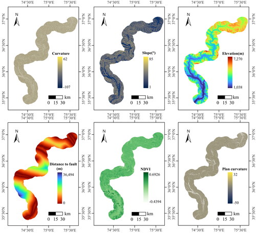
Figure 5. Continued LCFs.

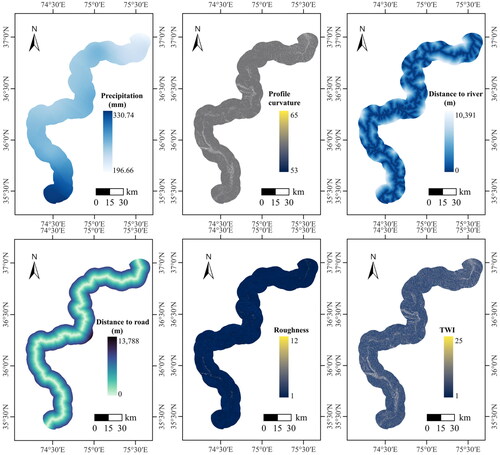
Figure 6. Continued LCFs.

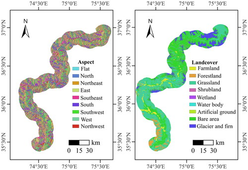
Table 2. Conditioning factors.

Factors	Sources	Category	Resolution
Lithology	GLiM (Hartmann and Moosdorf 2012)	Geology	/
Distance to fault	Global Active Earthquake Faults (https://www.arcgis.com/home)	Geology	/
	Spatial database of 1:5 Million International Geological Map of Asia (http://dcc.cgs.gov.cn/cn/)	Geology	/
Elevation	ALOS-PALSAR DEM (https://search.asf.alaska.edu)	Topography	12.5m
Curvature		Topography	12.5m
Plan curvature		Topography	12.5m
Profile curvature		Topography	12.5m
Aspect		Topography	12.5m
Slope		Topography	12.5m
Roughness		Topography	12.5m
TWI		Topography	12.5m
Precipitation	CRU TS 4.06 (https://crudata.uea.ac.uk/cru/data/hrg/cru_ts_4.06)	Hydrology	0.5°
Distance to river	OpenStreetMap	Hydrology	/
Landcover	Globaland30 (http://www.globallandcover.com/)	Other	30m
NDVI	Sentinel-2	Other	10m
Distance to road	OpenStreetMap	Other	/

NIR and Red represent the reflectance values in the near-infrared and red bands.

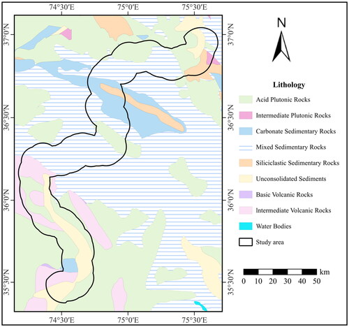
One of the significant intrinsic factors contributing to landslide occurrences in the study area is the unique internal geological characteristics, particularly the lithology (Guzzetti et al. 1996; Henriques et al. 2015). The predominant lithology within the study area consists of sedimentary rocks, including siliciclastic sedimentary rocks, unconsolidated sediments, mixed sedimentary rocks, and carbonate sedimentary rocks, collectively accounting for approximately 62% of the total area. Mixed sedimentary rocks are the most prevalent, covering approximately 38% of the study area. Additionally, the remaining lithology is predominantly igneous rocks, with acid plutonic rocks being the most common, occupying approximately 28% of the study area (Figure 7).

Figure 7. Lithological map.

2.3. Landslide susceptibility prediction models

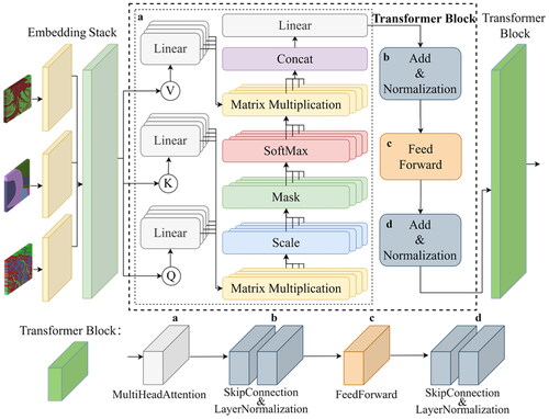
2.3.1. Feature fusion transformer

This study introduces FFTR to integrate the spatial features of all the conditioning factors (Figure 9). The conditioning factors are divided into two types for feature fusion: discrete features and continuous features. The discrete feature fusion includes landcover, lithology, and aspect (Figures 6 and 7). Before embedding coding, landcover and aspect (each with ten classes) are encoded with indices [1, 2, 3, …, 10], while lithology (with eight classes) is encoded using indices [1, 2, 3, …, 8]. The factors are initially inputted into their respective embedding layers for the fusion of discrete features (Figure 9).

For the fusion of continuous features, taking the processing of the landcover feature in the embedding layer as an example, the feature dimension outputted by the embedding layer is 16. Thus, the shape of the output from the embedding layer is (10, 16). These three discrete features are then inputted into the stack layer, resulting in a new shape of (10, 3, 16). Subsequently, the features are further processed in the transformer block for subsequent feature fusion. The ‘flatten’ layer transforms the multidimensional representation of discrete features into a one-dimensional form, effectively flattening the input. By doing so, the original input shape, such as (10, 3, 16), is reshaped to (10, 48). At this point, the fusion of discrete features is concluded (Figure 9).

Furthermore, some details still need clarification regarding the handling of discrete features. The key to the transformer block takes its foundation from implementing the attention mechanism (Figure 8). The essence of the attention mechanism is a process of addressing, where a query vector (Q) is given for the factor features. It computes the attention distribution concerning the key vectors (K) and applies it to the value vectors (V) to calculate the attention value. This study’s transformer block applies a multi-head self-attention mechanism based on Scaled Dot-Product Attention (Vaswani et al. 2017). The computation principle of the attention mechanism is as follows: (2) $$\mathrm{At}\mathrm{t}\mathit{ention}\left(Q,K,V\right)=\mathit{softmax}\left(\frac{Q{K}^T}{\sqrt{d_k}}V\right)$$(2)

Figure 8. Explanatory diagram of the transformer block.

where $\sqrt{d_k}$ represents the scale parameter.

Through utilizing Multi-Head Attention, the model is fragmented into multiple heads, ultimately establishing distinct subspaces. The Multi-Head Attention is accomplished by applying the Scaled Dot-Product Attention process H (in this study, H is set to 4) times and then combining the outputs (Vaswani et al. 2017). The input is processed through a linear transformation: (3) $$Q_i=Q{W}_i^Q,K_i=K{W}_i^K,V_i=V{W}_i^v,i=1,2,3,4$$(3)

After the linear transformation, the matrix multiplication and scale ($\sqrt{d_k}$) are performed between Q and V. The multi-head attention mechanism follows the following procedure: (4) $$\mathit{hea}{d}_i=\mathit{Attention}\left(Q_i,K_i,V_i\right),i=1,2,3,4$$(4) (5) $$\mathit{Mul}{t}_{i}H\mathit{ead}\left(Q,K,V\right)=\mathit{Concat}\left(\mathit{hea}{d}_1,\mathit{hea}{d}_2,\mathit{hea}{d}_3,\mathit{hea}{d}_4\right)W^O$$(5)

The data is normalized by transforming its mean to 0 and standard deviation to 1 by applying layer normalization (Ba et al. 2016). After normalization, the features are fed into the feedforward layer. The feedforward layer is formed by two linear transformations and a non-linear activation function, ReLU. The computation principle of the feedforward layer can be described as follows: (6) $$\mathit{FFN}\left(x\right)=\max \left(0,x{W}_1+b_1\right)W_2+b_2$$(6)

After another skip connection and layer normalization, the operation of a single transformer block is completed. In this study, a total of three blocks were utilized.

For the fusion of continuous features, the continuous features are expanded in dimension and then inputted into a concatenate layer to combine the dimensions. The resulting concatenated features are further passed through layer normalization for regularization. This operation ensures consistent scaling and reduces the impact of variations in the continuous feature distributions. The output shape after layer normalization is (1, 12). Thus, the fusion of continuous features is complete (Figure 9).

Figure 9. The framework of the FFTR.

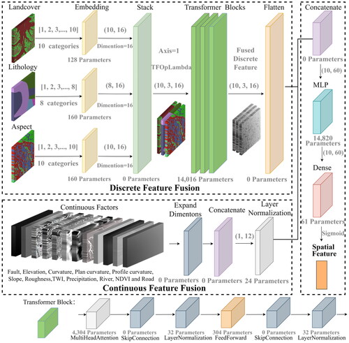
After completing these two fusion steps, the fusion output for discrete and continuous features is concatenated with the output shape (10, 60) and inputted into a concatenate layer. The concatenated features are then passed to a Multilayer Perceptron (MLP) (Taud and Mas 2018). In this study, two hidden layers are incorporated into the MLP architecture. The first hidden layer consists of 120 hidden units, while the second hidden layer consists of 60 hidden units. Batch normalization is utilized as the regularization method within the MLP to address the potential ‘Internal Covariate Shift’ issue (Ioffe and Szegedy 2015). Batch normalization operates at the batch level and normalizes each neuron individually. The output of the MLP is computed using the SELU activation function (Klambauer et al. 2017).

In the absence of batch normalization, the activation function can be represented as follows: (7) $$f\left(x\right)=\lambda \{\begin{array}{cc}\alpha \left(e^x\mathrm{ }\text{-}\mathrm{ }1\right),& x\le 0\\ x,& x>0\end{array}$$(7)

With the inclusion of batch normalization, the activation function layer can be represented as follows: (8) $$f\left(\mathit{batchNorm}\right(x\left)\right)=\lambda \{\begin{array}{cc}\alpha \left(e^x\mathrm{ }\text{-}\mathrm{ }1\right),& x\le 0\\ x,& x>0\end{array}$$(8)

The last layer of FFTR consists of a dense, fully connected layer that connects all neurons from the previous layer to every neuron in the current layer. The activation function applied in this layer is the sigmoid function. The output dimension of this layer is 1, indicating the fused spatial features are outputted as a single scalar value. (9) $$\mathit{sigmoid}\left(x\right)=\frac{1}{1+e^{-x}}$$(9)

The optimizer adapted is adaptive moment estimation (Adam) (Kingma and Ba 2014). The loss function is binary cross-entropy loss: (10) $$\mathit{Loss}=-\frac{1}{N}{\sum }_{i=1}^N{y}_i\hspace{0.17em}\log \hspace{0.17em}\left(p\left(y_i\right)\right)+\left(1-y_i\right)\hspace{0.17em}\log \hspace{0.17em}\left(1-p\left(y_i\right)\right)$$(10)

2.3.2. Feature fusion transformer and machine learning classifiers

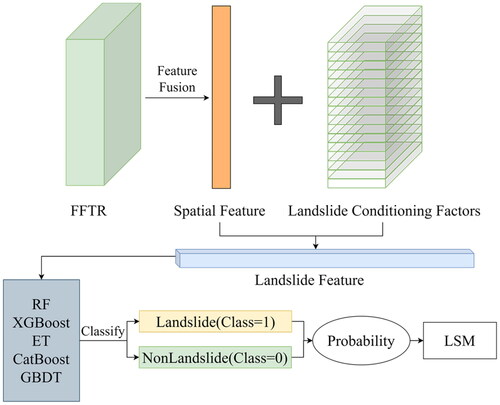
The fused spatial features obtained from the FFTR module are combined with the LCFs to generate the spatial feature of the landslide. Combining the abstract fused features derived from FFTR with the LCFs allows the susceptibility model’s learning perspective to encompass global and local features. This approach maximizes the effective exploration and utilization of the distinct characteristics inherent in all LCFs. These combined features are then utilized with RF, XGBoost, ET, CatBoost, and GBDT to classify the data into landslide and non-landslide instances. The final step in the process is to output the probabilities of landslide occurrence and generate susceptibility maps (Figure 10).

Figure 10. Feature fusion transformer and ML classifiers.

RF employs an ensemble learning technique combining multiple decision trees, culminating in a powerful classifier (Breiman 2001). It is known for its effectiveness in handling missing values and its ability to assess the importance of different features in the classification process. In this study, feature selection is accomplished using the Gini coefficient: (11) $$\mathit{Gini}\left(p\right)={\sum }_{k=1}^K{p}_k\left(1-p_k\right),\mathrm{ }k=1,2$$(11) p_k represents the probability that a sample belongs to the class labeled as k.

The Extra Trees (ET) algorithm is also an ensemble learning method that utilizes a set of decor-related decision trees for classification (Geurts et al. 2006). In contrast to RF, ET does not employ the bagging technique but instead uses all training samples for individual decision trees. Additionally, ET performs feature splits in a fully random feature selection strategy without using a random subset of features, reducing variance and preventing the undue influence of certain features. The feature splits in ET are also based on the Gini coefficient.

GBDT is a classifier that utilizes CART regression trees as its base learners. It is an iterative algorithm that constructs a set of weak learners and combines their outputs to generate the final prediction. GBDT can discover high-order relationships between features automatically. The feature splitting in GBDT is based on Friedman Mean Square Error (Friedman 2001). The loss function for classification is the logarithmic loss function, which is defined as follows: (12) $$L\left(y,f\left(x\right)\right)=-{\sum }_{k=1}^K{y}_k\hspace{0.17em}\log \hspace{0.17em}{p}_k\left(x\right)$$(12) p_k represents the probability that a sample belongs to the class labeled as k.

Under the framework of the GBDT algorithm, two notable improvements emerged: XGBoost and CatBoost. XGBoost introduces a novel technique that pre-sorts and stores the data, allowing for efficient reuse during subsequent computations (Chen and Guestrin 2016): (13) $$\widehat{{y_i}^t}={\sum }_{k=1}^t{f}_k\left(x_i\right)=\widehat{y_i^{\left(t¯1\right)}}+f_t\left(x_i\right)$$(13)

Denote $\widehat{{y_i}^t}$ as the predicted result of sample i after the t-th iteration, $\widehat{y_i^{\left(t¯1\right)}}$ as the predictions from the previous t-1 classifiers and $f_t\left(x_i\right)$ denotes the function of the t-th classifier.

CatBoost focuses on handling categorical features efficiently. It employs a specific type of decision tree called ‘oblivious trees’ as the base learners (Dorogush et al. 2018; Prokhorenkova et al. 2018). Typically, numerical representations are derived from categorical feature values via the application of the provided equation: (14) $$\mathit{target}=\frac{\mathit{countInClass}+\mathit{prior}}{\mathit{totalCount}+1}$$(14)

In the given equation, ‘countInClass’ stands for the total sample count in the current categorical feature value that has a label value of 1. ‘prior’ is the initial value of the numerator, which is determined based on the initial parameters. ‘totalCount’ refers to the overall count of samples with identical categorical feature values as the current sample incorporating the ongoing sample.

In this study, five evaluation metrics were employed. These indicators encompass accuracy, precision, recall, F₁-score, and AUC value (Ji et al. 2020).

2.4. Displacement velocity calculation

This study employed the PS-InSAR technique to calculate the displacement velocity within the study area. PS-InSAR is based on multi-scene SAR data in the same geographical region, which can detect Persistent Scatterer points unaffected by temporal and spatial baseline decorrelation. This technique offers significant temporal coverage for displacement monitoring, the capacity to mitigate atmospheric interference, and the capability to discern millimeter-scale displacement (Beladam et al. 2019).

The SAR data mainly utilized ascending and descending data from 2021 to 2023, totaling 100 scenes (Table 3).

Table 3. SAR data.

Data description	Ascending	Descending
Product	Sentinel-1 SLC
Band	C
Beam mode	IW
Polarization	VV
Path	27	107
Frame	111 and 116	468 and 473
Date	2021/05-2023/05	2021/05-2023/06
Number of images	50	50

2.5. Incorporation of displacement velocity with landslide susceptibility mapping

This study defines the PS-InSAR calculated displacement velocity into three levels to incorporate the outcomes of PS-InSAR into the landslide susceptibility predicted by the model. Regarding the landslide displacement velocity classification (Cruden and Varnes 1996), moderate, high, and very high landslide susceptibility levels were assigned.

More specifically, it is divided into these three intervals according to its displacement velocity distribution: (μ − σ, μ + σ) is moderate; (μ − 2σ, μ – σ] and [μ + σ, μ + 2σ) are high; the rest are very high. μ is the mean; σ is the standard deviation calculated as follows:

Finally, landslide susceptibility predictions missed by the model or predictions that differ from PS-InSAR calculations will be integrated.

3. Results

3.1. Comparison of landslide susceptibility prediction models

The fused spatial features obtained from the Features FFTR were utilized as input for machine learning classifiers, creating five combination models. The combination of FFTR and RF exhibited the most outstanding performance among these models. It achieved an AUC value of 94%. The accuracy of this model was measured at 87.31%, while precision, recall, and F₁-score were calculated as 87.21%, 88.02%, and 87.61%, respectively (Table 4).

Table 4. Evaluation results.

Methods	AUC	Accuracy	Precision	Recall	F1-score
FFTR-RF	94.00%	87.31%	87.21%	88.02%	87.61%
FFTR-ET	93.05%	85.12%	86.76%	83.87%	85.29%
FFTR-XGBoost	91.11%	83.87%	82.20%	87.25%	84.65%
FFTR-CatBoost	90.98%	82.22%	80.90%	85.25%	83.02%
FFTR-GBDT	90.06%	81.99%	82.89%	85.56%	84.20%

The results of this study demonstrate that the FFTR, integrating all LCFs, exhibited superior performance among all modules. The FFTR module achieved an AUC of 91.77%. It also gained an accuracy of 84.34%, precision of 84.96%, recall of 84.18%, and F₁-score of 84.57%, all of which ranked first among the baseline models in performance. Following FFTR, RF module attained an AUC of 89.18%. The remaining modules, ranked in descending order of performance, were XGBoost, ET, CatBoost, and GBDT (Table 5).

Table 5. Evaluation results.

Models	AUC	Accuracy	Precision	Recall	F1-score
FFTR	91.77%	84.34%	84.96%	84.18%	84.57%
RF (Hussain et al. 2022)	89.18%	81.99%	81.37%	83.87%	82.60%
XGBoost (Hussain et al. 2021)	88.92%	80.58%	79.85%	82.80%	81.30%
ET	87.95%	80.26%	79.56%	82.49%	81.00%
CatBoost	87.24%	78.70%	78.16%	80.80%	79.46%
GBDT	85.51%	78.47%	77.49%	81.41%	79.40%

Notably, incorporating FFTR in feature fusion led to an increase of 2.23% in AUC compared to using FFTR alone; when compared to RF alone, the AUC was improved by 4.82%. Remarkable enhancements in performance were observed across all evaluation metrics for the remaining modules as well. These findings underscore the significant improvements achieved by incorporating FFTR for feature fusion, further enhancing the overall performance of the models.

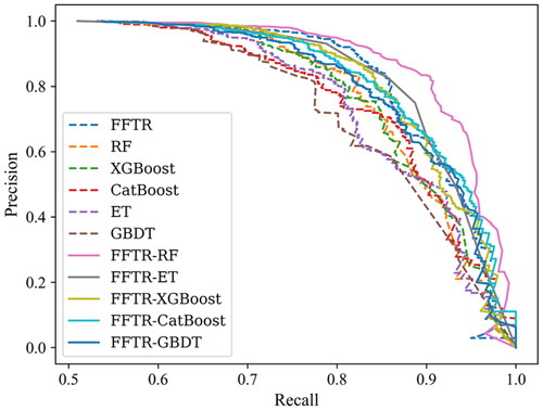
Based on the classification performance across all data, the FFTR-RF model demonstrates better results than other models with the highest AUC value. The larger area under the ROC curve suggests its superior ability to distinguish between positive and negative instances (Figure 11). Similarly, the larger area under the Precision-Recall (PR) curve indicates its better precision and recall trade-off (Figure 12). These results demonstrate that the FFTR-RF model exhibited the most optimal performance among the evaluated models regarding classification ability.

Figure 11. ROC curve of different models.

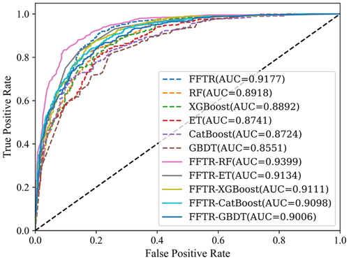
Figure 12. PR curve of different models.

3.2. Displacement velocity results

The PS-InSAR technique processes SAR data encompassing 100 scenes acquired between 2021 and 2023.

Two primary software packages were utilized: SARscape 5.6 and MATLAB-based SARPROZ.

For SARscape, the initial step generates a connectivity map and automatically selects the super-master image. After the interferometric process, the displacement velocity is obtained by completing two inversions and geocoding. Notably, a coherence threshold of 0.6 is applied.

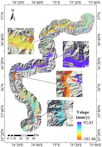
For SARPROZ, after the data input, co-registration is completed. In multi-image sparse points processing, the threshold is 0.6. The displacement velocity is output by geocoding. The displacement velocity along the slope in the study area was calculated. The velocity values of the displacement ranged from −101.46 mm/year to 92.03 mm/year within the study area, with a mean value of 1.68 mm/year and a standard deviation of 19.41 mm/year (Figure 13). Certain areas within the area exhibited high levels of deformation along the slope. These areas may signify the presence of potential landslide-prone areas.

Figure 13. Displacement velocity along the slope.

3.3. Landslide susceptibility mapping

After feeding all the LCFs into the model, the model outputted the probability of landslide occurrence, which was then used to classify the landslide susceptibility into five levels: very low (0 to 0.2), low (0.2 to 0.4), moderate (0.4 to 0.6), high (0.6 to 0.8), and very high (0.8 to 1) (Figure 14). The resolution is 30 m. The classification is based on the calculated probabilities, and each susceptibility level represents a different likelihood of landslide occurrence.

Figure 14. LSM results of different models.

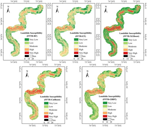
In all the landslide susceptibility maps, the central part of the study area exhibits higher susceptibility to landslides. Using the FFTR-RF model for LSM, the outputs demonstrate that the percentage of areas classified as low (including low and very low) is 57.64%, moderate is 29.45%, and high (including high and very high) is 12.91%. This distribution indicates that a portion of the study area is susceptible to landslide hazards, emphasizing the need for effective mitigation and management strategies in these high-risk areas.

For these five different landslide susceptibility maps, some comparisons were made in terms of displacement velocity results. More specifically, for the three susceptibility classes (moderate, high, and very high), the intersection ratio (IR) between the model-predicted results (m) and displacement velocity results (p) was calculated: (15) $$IR=\frac{m\cap P}{P}$$(15)

FFTR-RF displays the highest IR with the deformation calculation results computed from PS-InSAR, thus also establishing it as the top-performing model among these five (Table 6).

Table 6. IR evaluation results.

Name	FFTR-RF	FFTR-ET	FFTR-CatBoost	FFTR-GBDT	FFTR-XGBoost
IR	62.82%	58.85%	56.78%	45.33%	44.91%

Therefore, the FFTR-RF model with the best performance was chosen. The results from LSM within regions categorized as ‘moderate,’ ‘high,’ and ‘very high’ were integrated with the results obtained from PS-InSAR. Simultaneously, the displacement velocity was also categorized as ‘moderate,’ ‘high,’ and ‘very high.’ The union of the results for these three categories from both the FFTR-RF model and PS-InSAR was taken. For ‘high’ and ‘very high’, in cases where there is inconsistency in the category values for a particular pixel, the value from PS-InSAR was adopted for that pixel.

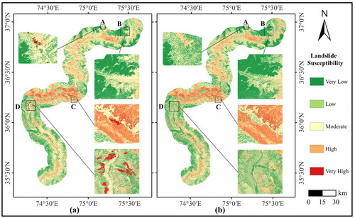
The final LSM results are generated by integrating the FFTR-RF model’s predictive outcomes and the PS-InSAR calculated results (Figure 15). Notably, in regions A, B, C, and D, it is evident that the FFTR-RF model exhibits misclassification and omissions for high and very high susceptibility results. In region B, some moderate susceptibility results also show misclassifications and omissions. In summary, integrating the results from PS-InSAR has significantly enhanced the mapping comprehensiveness of LSM.

Figure 15. LSM results. (a) is the final integrated LSM result; (b) is the LSM result of FFTR-RF.

3.4. The importance of LCFs

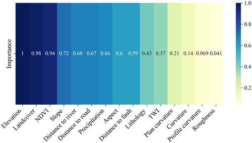
The RF algorithm performed feature importance ranking for all features, enabling a feature importance analysis of LCFs. According to the analysis results, elevation (100%) was found to have the greatest impact on landslide occurrence. Subsequently, landcover (97.71%) and NDVI (94.11%) were identified as factors significantly influencing landslide occurrence. Slope (71.86%), distance to river (67.66%), distance to road (67.46%), and precipitation (65.57%) were found to have a moderate level of impact on landslide occurrence. Factors such as aspect (59.55%), distance to fault (59.27%), lithology (43.03%), and TWI (37.31%) were determined to have an impact on landslide occurrence below 60%. Moreover, plan curvature (20.85%), curvature (14.27%), profile curvature (6.92%), and roughness (4.14%) were found to have an impact below 30% (Figure 16).

Figure 16. LCFs importance heatmap.

4. Discussion

4.1. Newly identified landslide-prone regions

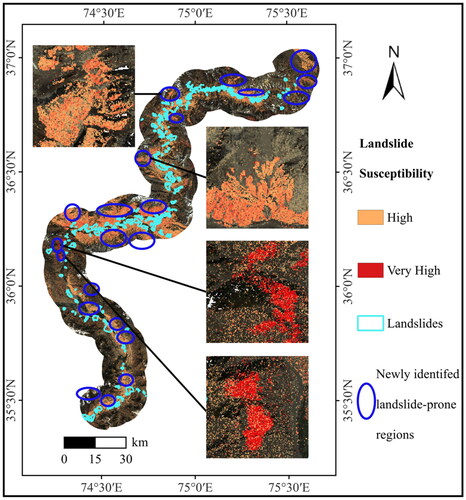
The areas classified as high and very high in landslide susceptibility in the final integrated LSM result were overlaid to identify new areas with landslide propensity along the KKH (Figure 17). The high and very high susceptibility areas likely indicate areas with a tendency for landslides. Furthermore, some of these areas are not included in the landslide inventory compiled in this study, suggesting that they may represent areas with a high potential for future landslides. We recommend regular monitoring and timely preventive measures for these areas with identified landslide propensity to mitigate potential risks.

Figure 17. Landslide-prone regions.

4.2. Feature fusion transformer parameters

The parameters configuration for FFTR in this study is presented in Table 7. Notably, the multi-head attention mechanism plays a vital role in capturing contextual information related to landslides, enabling the model to learn various contextual patterns (Vaswani et al. 2017). The number of heads in the multi-head attention mechanism is critical as it determines the model’s ability to capture a wide range of relevant features and enhance its expressive capacity. However, a larger number of heads increases model parameters and computational complexity. In this study, four was chosen as the number of heads, striking a balance between capturing diverse contextual information and maintaining computational efficiency.

Table 7. Parameters.

Parameters	values
Learning rate	0.001
Weight decay	0.0001
Dropout rate	0.05
Batch size	20
Number of epochs	30
Number of transformer blocks	3
Number of heads in the multi-head attention	4
Number of MLP blocks	2
Optimizer	‘Adam’

Furthermore, the Adam optimizer was employed, and the ‘weight decay’ parameter was utilized for weight decay regularization. Weight decay helps control the model’s complexity by adding a regularization term to the loss function, preventing overfitting (Loshchilov and Hutter 2017). The ‘weight decay’ parameter applies L2 regularization to the model’s weights in the Adam optimizer. During each weight update, the ‘weight decay’ value is multiplied by the weights, gradually reducing the weights. Notably, a ‘weight decay’ value greater than 0.001 led to underfitting in this study. Hence, a ‘weight decay’ value of 0.001 was selected.

The overall model comprises 29,369 parameters, with the transformer blocks accounting for 14,016 parameters.

4.3. Sensitivity of FFTR-ML

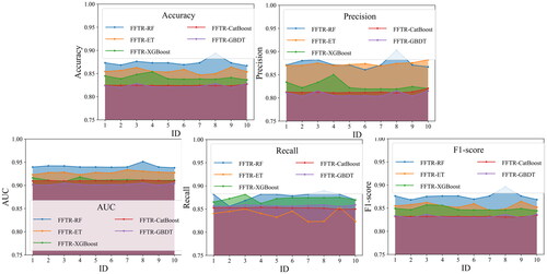
The Monte Carlo Cross-Validation method assessed the model’s data sensitivity and generalization capability (Xu and Liang 2001). The dataset was randomly partitioned in each iteration, with 70% of the data allocated to training, 20% to validation, and the remaining 10% excluded from analysis. This process was repeated ten times to perform model training and validation. Using metrics such as AUC, accuracy, precision, recall, and F₁-score as evaluation criteria, the average values of these metrics were calculated from the ten shuffle-split results and visualized using a radar chart (Figure 18). AUC, accuracy, precision, recall, and F₁-score were meticulously recorded for each of the ten cross-validation runs (Figure 19).

Figure 18. Average evaluation metrics.

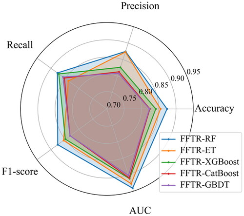
Figure 19. Evaluation metric for each shuffle split.

The results unequivocally demonstrate that, compared to other models, the FFTR-RF model exhibited the highest performance, indicating its robust generalization ability.

4.4. Mapping discrepancies in FFTR-XGBoost

Among the diverse model mapping outcomes, it is evident that the LSM generated by the FFTR-XGBoost model exhibits pronounced dissimilarity compared to those produced by other models (Figure 14). In the IR result, the FFTR-XGBoost value is the lowest (Table 6). A crucial insight from these mapping results highlights that the moderate category, characterized by probabilities ranging from 0.4 to 0.6, represents the smallest proportion among the five models, accounting for only 7.56% of pixel values.

The scarcity of outcomes in the moderate category can be attributed to the unique nature of the XGBoost model. Notably, each weak learner in XGBoost is sequentially fitted based on the preceding weak learner, with their predictions ultimately weighted and aggregated to formulate the final prediction. The training process of XGBoost explicitly optimizes the classification results of samples (refer to Equation (13)(13) $$\widehat{{y_i}^t}={\sum }_{k=1}^t{f}_k\left(x_i\right)=\widehat{y_i^{\left(t¯1\right)}}+f_t\left(x_i\right)$$(13) ) rather than directly optimizing the probability values. Consequently, the loss function incorporates penalties for misclassified samples, fostering a tendency for the model to favor more definitive predictions rather than assigning ambiguous probabilities around 0.5.

In essence, XGBoost exhibits a predisposition towards outcomes with either low or high probabilities, thereby resulting in a diminished number of outcomes falling within the moderate category. Therefore, the mapping results exhibit significant differences compared to the other maps. With the high and very high categories having similar proportions in all model results, the lowest percentage of the moderate category contributes to its lowest IR values.

4.5. Future research

This study conducted LSM along the KKH using a series of landslide conditioning factors to analyze the spatial distribution of susceptibility. However, spatial LSM still has limitations in timely alerts for areas at risk of potential landslides. Therefore, future research will continue to explore LSM on a temporal scale.

In addition, landslides also encompass different categories, each with distinct prevention and control measures. Thus, considering these categories in LSM is a prospective avenue for future research. In the area around KKH, the effect of glaciers or snow melting on landslide hazards in the summer as the temperature rises is not included in this study. Subsequent research will continue to improve the susceptibility mapping by considering the effect of snow and ice meltwater on landslides.

5. Conclusions

In recent decades, landslide disasters have profoundly impacted the KKH, a pivotal economic conduit linking China and Pakistan. Consequently, this article employs a comprehensive array of LCFs, including lithology, distance to fault, elevation, curvature, plan curvature, profile curvature, aspect, slope, roughness, TWI, precipitation, distance to river, landcover, NDVI, and distance to road. Based on the above data, a landslide inventory is compiled, utilizing a 10-kilometer buffer zone of KKH. Subsequently, landslide susceptibility models are formulated. Finally, displacement velocity is incorporated for LSM.

The substantive contributions of this article are listed as follows:

1. To enhance the exploration of spatial patterns and interrelationships between LCFs and landslide data, a transformer-based FFTR feature fusion module is introduced. The 15 LCFs are categorized into continuous and discrete data subsets, facilitating effective feature fusion. The fused feature is subsequently fed into five distinct machine learning classifiers: RF, ET, GBDT, XGBoost, and CatBoost. Comprehensive evaluation metrics collectively indicate that the FFTR-RF model yields the most superior outcomes for landslide susceptibility prediction.

2. To capture the dynamic deformations of landslides, this article utilizes the PSInSAR technique to monitor surface deformations continuously. Employing a SAR dataset of 100 images from 2021 to 2023, the displacement velocity in the study area is calculated.

3. Upon the two points mentioned above, and to enhance the comprehensiveness of susceptibility mapping, this study categorizes displacement velocity into three distinct classes: moderate, high, and very high. These classifications are then integrated into the susceptibility results generated by the model. This approach contributes to the derivation of the final susceptibility map.

The method proposed in this study enhances the accuracy of landslide warnings and assists governmental and societal institutions in developing robust mechanisms for landslide disaster prevention and early warning.

Acknowledgments

Our heartfelt appreciation to the editor and reviewers for their invaluable comments and constructive suggestions, significantly elevating the paper’s quality.

Data availability statement

To access the data provided in the study, please get in touch with the lead and corresponding author.

Disclosure statement

No potential conflict of interest was reported by the author(s).

Additional information

Funding

This work was supported by the Key Projects of Foundation Improvement Program under Grant [2022JCJQZD21500], National Natural Science Foundation of China under Grant [41871305, 42122025] and Opening Fund of Key Laboratory of Geological Survey and Evaluation of Ministry of Education under Grant [GLAB2022ZR06].

References

- Abid M, Ashfaq A. 2015. CPEC: challenges and opportunities for Pakistan. Pak Vision. 16(2):142–169.
- Ali S, Biermanns P, Haider R, Reicherter K. 2019. Landslide susceptibility mapping by using a geographic information system (GIS) along the China–Pakistan Economic Corridor (Karakoram Highway), Pakistan. Nat Hazards Earth Syst Sci. 19(5):999–1022. doi: 10.5194/nhess-19-999-2019.
- Amatriain X. 2023. Transformer models: an introduction and catalog. arXiv preprint arXiv: 07730.
- Ba JL, Kiros JR, Hinton GE. 2016. Layer normalization. arXiv preprint arXiv: 06450.
- Beladam O, Balz T, Mohamadi B, Abdalhak M. 2019. Using PS-INSAR with sentinel-1 images for deformation monitoring in northeast Algeria. Geosciences. 9(7):315. doi: 10.3390/geosciences9070315.
- Brabb EE. 1985. Innovative approaches to landslide hazard and risk mapping. International Landslide Symposium Proceedings, Toronto, Canada. p. 17–22.
- Breiman L. 2001. Random forests. Mach Learn. 45(1):5–32. doi: 10.1023/A:1010933404324.
- Bui DT, Tsangaratos P, Nguyen VT, Van Liem N, Trinh PT. 2020. Comparing the prediction performance of a deep learning neural network model with conventional machine learning models in landslide susceptibility assessment. Catena. 188:104426. doi: 10.1016/j.catena.2019.104426.
- Chen T, Guestrin C. 2016. Xgboost: a scalable tree boosting system. Proceedings of the 22nd ACM SIGKDD International Conference on Knowledge Discovery and Data Mining. p. 785–794.
- Chen Y, Ming D, Ling X, Lv X, Zhou C. 2021. Landslide susceptibility mapping using feature fusion-based CPCNN-ML in Lantau Island, Hong Kong. IEEE J Sel Top Appl Earth Observat Remote Sens. 14:3625–3639. doi: 10.1109/JSTARS.2021.3066378.
- Cruden DM, Varnes DJ. 1996. Landslides: investigation and mitigation. Chapter 3-Landslide Types Processes. Transport Res Board Special Rep. 247:030906208X.
- Di Napoli M, Carotenuto F, Cevasco A, Confuorto P, Di Martire D, Firpo M, Pepe G, Raso E, Calcaterra D. 2020. Machine learning ensemble modelling as a tool to improve landslide susceptibility mapping reliability. Landslides. 17(8):1897–1914. doi: 10.1007/s10346-020-01392-9.
- Dorogush AV, Ershov V, Gulin A. 2018. CatBoost: gradient boosting with categorical features support. arXiv preprint arXiv: 11363.
- Dou J, Yunus AP, Tien Bui D, Sahana M, Chen CW, Zhu Z, Wang W, Pham BT. 2019. Evaluating GIS-based multiple statistical models and data mining for earthquake and rainfall-induced landslide susceptibility using the LiDAR DEM. Remote Sens. 11(6):638. doi: 10.3390/rs11060638.
- El Jazouli A, Barakat A, Khellouk R. 2019. GIS-multicriteria evaluation using AHP for landslide susceptibility mapping in Oum Er Rbia high basin (Morocco). Geoenviron Disasters. 6(1):1–12. doi: 10.1186/s40677-019-0119-7.
- Fang Z, Wang Y, Peng L, Hong H. 2020. Integration of convolutional neural network and conventional machine learning classifiers for landslide susceptibility mapping. Comput Geosci. 139:104470. doi: 10.1016/j.cageo.2020.104470.
- Fayaz A, Latif M, Khan K. 1985. Landslide evaluation and stabilization between Gilgit and Thakot along the Karakoram Highway. Geological Survey of Pakistan, Islamabad, Pakistan.
- Friedman JH. 2001. Greedy function approximation: a gradient boosting machine. Ann Stat. 29(5):1189–1232.
- Gaidzik K, Ramírez-Herrera MT. 2021. The importance of input data on landslide susceptibility mapping. Sci Rep. 11(1):19334. doi: 10.1038/s41598-021-98830-y.
- Geurts P, Ernst D, Wehenkel L. 2006. Extremely randomized trees. Mach Learn. 63(1):3–42. doi: 10.1007/s10994-006-6226-1.
- Gupta SK, Shukla DP. 2023. Handling data imbalance in machine learning based landslide susceptibility mapping: a case study of Mandakini River Basin, North-Western Himalayas. Landslides. 20(5):933–949. doi: 10.1007/s10346-022-01998-1.
- Guzzetti F, Cardinali M, Reichenbach P. 1996. The influence of structural setting and lithology on landslide type and pattern. Environ Eng Geosci. II(4):531–555. doi: 10.2113/gseegeosci.II.4.531.
- Guzzetti F, Carrara A, Cardinali M, Reichenbach P. 1999. Landslide hazard evaluation: a review of current techniques and their application in a multi-scale study, Central Italy. Geomorphology. 31(1-4):181–216. doi: 10.1016/S0169-555X(99)00078-1.
- Guzzetti F, Mondini AC, Cardinali M, Fiorucci F, Santangelo M, Chang KT. 2012. Landslide inventory maps: new tools for an old problem. Earth-Sci Rev. 112(1–2):42–66. doi: 10.1016/j.earscirev.2012.02.001.
- Hartmann J, Moosdorf N. 2012. The new global lithological map database GLiM: a representation of rock properties at the Earth surface. Geochem Geophys Geosyst. 13(12):1–37. doi: 10.1029/2012GC004370.
- Henriques C, Zêzere JL, Marques F. 2015. The role of the lithological setting on the landslide pattern and distribution. Eng Geol. 189:17–31. doi: 10.1016/j.enggeo.2015.01.025.
- Huang F, Cao Z, Guo J, Jiang SH, Li S, Guo Z. 2020. Comparisons of heuristic, general statistical and machine learning models for landslide susceptibility prediction and mapping. Catena. 191:104580. doi: 10.1016/j.catena.2020.104580.
- Huang F, Xiong H, Yao C, Catani F, Zhou C, Huang J. 2023a. Uncertainties of landslide susceptibility prediction considering different landslide types. JRMGE. 15(11):2954–2972. doi: 10.1016/j.jrmge.2023.03.001.
- Huang F, Yao C, Liu W, Li Y, Liu X. 2018. Landslide susceptibility assessment in the Nantian area of China: a comparison of frequency ratio model and support vector machine. Geomat Natl Hazards. 9(1):919–938. doi: 10.1080/19475705.2018.1482963.
- Huang F, Zhang J, Zhou C, Wang Y, Huang J, Zhu L. 2020b. A deep learning algorithm using a fully connected sparse autoencoder neural network for landslide susceptibility prediction. Landslides. 17(1):217–229. doi: 10.1007/s10346-019-01274-9.
- Huang W, Ding M, Li Z, Yu J, Ge D, Liu Q, Yang J. 2023. Landslide susceptibility mapping and dynamic response along the Sichuan-Tibet transportation corridor using deep learning algorithms. Catena. 222:106866. doi: 10.1016/j.catena.2022.106866.
- Huang Y, Zhao L. 2018. Review on landslide susceptibility mapping using support vector machines. Catena. 165:520–529. doi: 10.1016/j.catena.2018.03.003.
- Hussain MA, Chen Z, Wang R, Shoaib M. 2021. PS-InSAR-based validated landslide susceptibility mapping along Karakorum Highway, Pakistan. Remote Sens. 13(20):4129. doi: 10.3390/rs13204129.
- Hussain MA, Chen Z, Zheng Y, Shoaib M, Shah SU, Ali N, Afzal Z. 2022. Landslide susceptibility mapping using machine learning algorithm validated by persistent scatterer In-SAR technique. Sensors. 22(9):3119. doi: 10.3390/s22093119.
- Hussain S, Pan B, Afzal Z, Ali M, Zhang X, Shi X, Ali M. 2023. Landslide detection and inventory updating using the time-series InSAR approach along the Karakoram Highway, Northern Pakistan. Sci Rep. 13(1):7485. doi: 10.1038/s41598-023-34030-0.
- Ioffe S, Szegedy C. 2015. Batch normalization: accelerating deep network training by reducing internal covariate shift. International Conference on Machine Learning. p. 448–456.
- Javaid U. 2016. Assessing CPEC: potential threats and prospects. J Res Soc Pak. 53(2):254–269.
- Ji S, Yu D, Shen C, Li W, Xu Q. 2020. Landslide detection from an open satellite imagery and digital elevation model dataset using attention boosted convolutional neural networks. Landslides. 17(6):1337–1352. doi: 10.1007/s10346-020-01353-2.
- Jiang Z, Wang M, Liu K. 2023. Comparisons of convolutional neural network and other machine learning methods in landslide susceptibility assessment: a case study in Pingwu. Remote Sens. 15(3):798. doi: 10.3390/rs15030798.
- Khalil U, Imtiaz I, Aslam B, Ullah I, Tariq A, Qin S. 2022. Comparative analysis of machine learning and multi-criteria decision making techniques for landslide susceptibility mapping of Muzaffarabad district. Front Environ Sci. 10:1–19. doi: 10.3389/fenvs.2022.1028373.
- Khan K, Fayaz A, Hussain M, Latif M. 2003. Landslides problems and their mitigation along the Karakoram highway. Geological Survey of Pakistan: Islamabad, Pakistan.
- Khan K, Fayaz A, Latif M, Wazir A. 1986. Rock and debris slides between Khunjrab pass and Gilgit along the Karakoram highway. Geological Survey of Pakistan, Islamabad, Pakistan.
- Khan S, Liu G. 2019. The China–Pakistan economic corridor (CPEC): challenges and prospects. Area Develop. 4(4):466–473. doi: 10.1080/23792949.2018.1534549.
- Kingma DP, Ba J. 2014. Adam: a method for stochastic optimization. arXiv preprint arXiv:1412.6980.
- Klambauer G, Unterthiner T, Mayr A, Hochreiter S. 2017. Self-normalizing neural networks. Adv Neural Inform Process Syst. 30:1–10.
- Kulsoom I, Hua W, Hussain S, Chen Q, Khan G, Shihao D. 2023. SBAS-InSAR based validated landslide susceptibility mapping along the Karakoram Highway: a case study of Gilgit-Baltistan, Pakistan. Sci Rep. 13(1):3344. doi: 10.1038/s41598-023-30009-z.
- Li B, Liu K, Wang M, He Q, Jiang Z, Zhu W, Qiao N. 2022. Global dynamic rainfall-induced landslide susceptibility mapping using machine learning. Remote Sens. 14(22):5795. doi: 10.3390/rs14225795.
- Loche M, Alvioli M, Marchesini I, Bakka H, Lombardo L. 2022. Landslide susceptibility maps of Italy: lesson learnt from dealing with multiple landslide types and the uneven spatial distribution of the national inventory. Earth-Sci Rev. 232:104125. doi: 10.1016/j.earscirev.2022.104125.
- Loshchilov I, Hutter F. 2017. Decoupled weight decay regularization. arXiv preprint arXiv: 05101.
- Lv L, Chen T, Dou J, Plaza A. 2022. A hybrid ensemble-based deep-learning framework for landslide susceptibility mapping. Int J Appl Earth Obs. 108:102713. doi: 10.1016/j.jag.2022.102713.
- Melchiorre C, Matteucci M, Remondo J. 2006. Artificial neural networks and robustness analysis in landslide susceptibility zonation. The 2006 IEEE International joint conference on neural network proceedings. p. 4375–4381. doi: 10.1109/IJCNN.2006.247036.
- Merghadi A, Yunus AP, Dou J, Whiteley J, Thaipham B, Bui DT, Avtar R, Abderrahmane B. 2020. Machine learning methods for landslide susceptibility studies: a comparative overview of algorithm performance. Earth-Sci Rev. 207:103225. doi: 10.1016/j.earscirev.2020.103225.
- Mondini AC, Guzzetti F, Chang KT, Monserrat O, Martha TR, Manconi A. 2021. Landslide failures detection and mapping using synthetic aperture radar: past, present and future. Earth-Sci Rev. 216:103574. doi: 10.1016/j.earscirev.2021.103574.
- Ngo PTT, Panahi M, Khosravi K, Ghorbanzadeh O, Kariminejad N, Cerda A, Lee S. 2021. Evaluation of deep learning algorithms for national scale landslide susceptibility mapping of Iran. Geosci Front. 12(2):505–519. doi: 10.1016/j.gsf.2020.06.013.
- Nilofar M, Jiang WS, Ishtiaque M. 2014. The growing economic ties between Pakistan and china and its impact on the economy of Pakistan. IJRHAL. 2(12):49–54.
- Prokhorenkova L, Gusev G, Vorobev A, Dorogush AV, Gulin A. 2018. CatBoost: unbiased boosting with categorical features. NeurIPS. 31:1–11.
- Qing F, Zhao Y, Meng X, Su X, Qi T, Yue D. 2020. Application of machine learning to debris flow susceptibility mapping along the China–Pakistan Karakoram highway. Remote Sens. 12(18):2933. doi: 10.3390/rs12182933.
- Rashid B, Iqbal J, Su LJ. 2020. Landslide susceptibility analysis of Karakoram highway using analytical hierarchy process and scoops 3D. J Mt Sci. 17(7):1596–1612. doi: 10.1007/s11629-018-5195-8.
- Rehman MU, Zhang Y, Meng X, Su X, Catani F, Rehman G, Yue D, Khalid Z, Ahmad S, Ahmad I. 2020. Analysis of landslide movements using interferometric synthetic aperture radar: a case study in Hunza-Nagar Valley, Pakistan. Remote Sens. 12(12):2054. doi: 10.3390/rs12122054.
- Roy J, Saha S, Arabameri A, Blaschke T, Bui DT. 2019. A novel ensemble approach for landslide susceptibility mapping (LSM) in Darjeeling and Kalimpong districts, West Bengal, India. Remote Sens. 11(23):2866. doi: 10.3390/rs11232866.
- Searle M, Khan MA, Fraser J, Gough S, Jan MQ. 1999. The tectonic evolution of the Kohistan‐Karakoram collision belt along the Karakoram Highway transect, north Pakistan. Tectonics. 18(6):929–949. doi: 10.1029/1999TC900042.
- Su X-J, Zhang Y, Meng X-M, Yue D-X, Ma J-H, Guo F-Y, Zhou Z-Q, Rehman MU, Khalid Z, Chen G, et al. 2021. Landslide mapping and analysis along the China-Pakistan Karakoram Highway based on SBAS-InSAR detection in 2017. J Mt Sci. 18(10):2540–2564. doi: 10.1007/s11629-021-6686-6.
- Su X, Zhang Y, Meng X, Rehman MU, Khalid Z, Yue D. 2022. Updating inventory, deformation, and development characteristics of landslides in Hunza Valley, NW Karakoram, Pakistan by SBAS-InSAR. Remote Sens. 14(19):4907. doi: 10.3390/rs14194907.
- Taud H, Mas J. 2018. Multilayer perceptron (MLP). Geomatic approaches for modeling land change scenarios. p. 451–455.
- Vaswani A, Shazeer N, Parmar N, Uszkoreit J, Jones L, Gomez AN, Kaiser Ł, Polosukhin I. 2017. Attention is all you need. NeurIPS. 30:1–11.
- Wang Y, Fang Z, Hong H. 2019. Comparison of convolutional neural networks for landslide susceptibility mapping in Yanshan County, China. Sci Total Environ. 666:975–993. doi: 10.1016/j.scitotenv.2019.02.263.
- Wang Y, Fang Z, Wang M, Peng L, Hong H. 2020. Comparative study of landslide susceptibility mapping with different recurrent neural networks. Comput Geosci. 138:104445. doi: 10.1016/j.cageo.2020.104445.
- Whiteley J, Chambers J, Uhlemann S, Wilkinson PB, Kendall J. 2019. Geophysical monitoring of moisture‐induced landslides: a review. Rev Geophys. 57(1):106–145. doi: 10.1029/2018RG000603.
- Xu QS, Liang YZ. 2001. Monte Carlo cross validation. Chemom Intell Lab Syst. 56(1):1–11. doi: 10.1016/S0169-7439(00)00122-2.
- Yang J, Li C, Zhang P, Dai X, Xiao B, Yuan L, Gao J. 2021. Focal attention for long-range interactions in vision transformers. NeurIPS. 34:30008–30022.
- Yang T, Li Q, Chen X, Yin G, Li LH, De Maeyer P. 2020. Evaluation of spatiotemporal variability of temperature and precipitation over the Karakoram Highway region during the cold season by a Regional Climate Model. J Mt Sci. 17(9):2108–2122. doi: 10.1007/s11629-019-5772-5.
- Ye P, Yu B, Chen W, Liu K, Ye L. 2022. Rainfall-induced landslide susceptibility mapping using machine learning algorithms and comparison of their performance in Hilly area of Fujian Province, China. Nat Hazards. 113(2):965–995. doi: 10.1007/s11069-022-05332-9.
- Yixuetao SY, Shao P. 2021. An inventory dataset of the typical rockfalls and landslides in CPEC from 1970 to 2020. V2.
- Zhang H, Song Y, Xu S, He Y, Li Z, Yu X, Liang Y, Wu W, Wang Y. 2022. Combining a class-weighted algorithm and machine learning models in landslide susceptibility mapping: a case study of Wanzhou section of the Three Gorges Reservoir, China. Comput Geosci. 158:104966. doi: 10.1016/j.cageo.2021.104966.
- Zhang H, Yin C, Wang S, Guo B. 2023. Landslide susceptibility mapping based on landslide classification and improved convolutional neural networks. Comput Geosci. 116(2):1931–1971.
- Zhao C, Kang Y, Zhang Q, Lu Z, Li B. 2018. Landslide identification and monitoring along the Jinsha River catchment (Wudongde reservoir area), China, using the InSAR method. Remote Sens. 10(7):993. doi: 10.3390/rs10070993.
- Zheng S, Lu J, Zhao H, Zhu X, Luo Z, Wang Y, Fu Y, Feng J, Xiang T, Torr PH. 2021. Rethinking semantic segmentation from a sequence-to-sequence perspective with transformers. Proceedings of the IEEE/CVF Conference on Computer Vision and Pattern Recognition. p. 6881–6890.
- Zimmerman T. 2015. The New Silk Roads: China, the US, and the Future of Central Asia: Center on International Cooperation New York NY, USA.