The assessment of soil organic matter in the KwaZulu-natal province of South Africa and its relationship to spectroscopy data

Abstract

Soil organic matter (SOM) is made up of decomposing biotic material in various stages, as well as compounds generated by plant roots and soil organisms—it helps the soil’s biophysical functions. Laboratory spectroscopy, for example, provides a novel technique to analyse SOM content because it is both cost and time-efficient. Because of its composition and biophysical features, SOM has a distinct spectral reflectance; this relationship has been effectively exploited to estimate and predict SOM. The purpose of this study is to investigate the link between SOM concentration and laboratory-based soil spectral reflectance in the Emakhosaneni subplace of uThukela District, KwaZulu-Natal, South Africa. We collected 13 random soil samples from each of the four major land use types (agricultural, residential, eroded land, and rangeland), totalling 52 samples. To assess the SOM content, we oven-dried the materials overnight (105 °C), crushed them, sieved them (1 mm), and analysed them using the Walkley-Black method. The spectral reflectance of the soil samples was then acquired using the Analytical Spectral Device (ASD) FieldSpec3 and pre-processed for noise reduction before analysis. We found that the area’s average SOM content was 2.19%, with agricultural land having the greatest average SOM content (2.98%), followed by rangeland (2.46%), residential (1.77%), and eroded land area (1.56%). However, the average reflectance of the spectra was higher on eroded areas and decreased to a minimum on agricultural areas. This is attributed to the relationship between soil colour and SOM. Correlation analysis demonstrated a moderately negative relationship between SOM concentration and spectral reflectance over the whole spectral range covered (400–2400 nm). Our partial least squares regression analysis revealed that pre-processed spectra data models (FDT; R² = 0.46 and SG; R² = 0.34) performed better than raw data models, in both calibration and validation data sets, respectively. Despite the influence of noise on raw data model performance, they modestly predicted SOM content, particularly on the validation data set. However, the developed model cannot be used due to the very low coefficient of determination. Our results highlight the importance of spectroscopy to assess SOM content, and further research can be carried out on a larger scale.

Keywords:

• SOM
• spectroscopy
• PLSR model
• raw spectra
• pre-processed spectra

1. Introduction

Soil organic matter (SOM) is an important determinant of soil health and function (Adeline et al. 2017), and its amount varies as a consequence of plant tissue, microorganisms, animal residue and their different stages of breakdown. SOM formation is thus primarily a biological process that improves above ground biomass (Zhao et al. 2023), which contributes to the vitality and function of terrestrial ecosystems (Adeline et al. 2017). In this way, SOM is closely related to soil organic carbon (SOC) as its composition of organic compounds is highly enriched in carbon (Ayala Izurieta et al. 2022). As such, SOM is of great importance to the global carbon cycle and food production (Luo et al. 2022), making it an indispensable indicator to assess soil deterioration, which seriously threaten agricultural and ecological performance as well as environment safety (Obalum et al. 2017). Accurate quantification and characterisation of SOM is therefore crucial for a variety of strategic management decisions related to agricultural production and land sustainability.

Several innovative methods have been developed to measure and estimate SOM content in soils (Santoiemma 2018). Commonly used methods are laboratory-based and include; the Walkley-Black, Loss On Ignition, Automated dry combustion, and Humic matter methods (Roper et al. 2019). However, these methods can be costly at times and necessitate a longer analysis period, particularly when the study areas are big and substantial soil sampling is required. While these methods can measure SOM, remote sensing instruments offer several advantages, including time and cost savings, larger coverage, and non-destructive and quick data gathering, all of which can improve traditional methods (Wang et al. 2017). One such approach is spectroscopy, which has unique and innovative capabilities for determining SOM content (Hong et al. 2018b).

Currently, spectroscopy is being used in the field (Angelopoulou et al. 2020) and in the laboratory (Jia et al. 2023) to measure the Soil Organic Carbon and Soil Organic Matter reflectance spectra produced when features emit electromagnetic radiation (EMR) (Van der Meer 2018). The acquisition setup for these methods is significantly different, as measurements in the field are obtained under natural conditions, while measurements in the laboratory are performed under controlled conditions (Roudier et al. 2017). In the latter, the impact of environmental factors is minimized, and measurements are performed under artificial illumination instead of solar illumination in the field. This greatly influences the choice of the spectroscopy type, with availability and the feature of interest being additional considerations. Laboratory spectroscopy is generally preferred for soil analysis, and Wang et al. (2017) attribute this to the high spectral resolution, convenience, and controllability. Our emphasis in this study is on the quantification of SOM using laboratory-based spectroscopy.

Laboratory spectroscopy for SOM estimation is increasingly and successfully used in several regions of the world, a practice that has greatly facilitated our understanding of the soil system and the evaluation of its quality (Rossel et al. 2006). In this respect, Hong et al. (2019) established a good correlation between SOM and wavelengths in the visible (VIS) and near-infrared (NIR) channels. Wang et al. (2017) asserted that bands in the region of 440, 560, 625, 740 and 1336 nm are optimal spectral bands for SOM estimation under laboratory conditions. Liu et al. (2009) confirmed that the reflection between the 620 nm to 810 nm region is related to the SOM and that the highest correlation coefficient is in the 710 nm region of the spectrum. Again, He et al. (2009) showed a very close agreement between the VIS bands and the SOM, thus allowing SOM to be detectable within the VIS region of the electromagnetic spectrum. Such studies demonstrated the strategic bands in the successful estimation and characterization of SOM content using spectroscopy, particularly under laboratory conditions.

South Africa is no exception to countries with partly deficient SOM issues, as Du Preez et al. (2011) showed that some parts of the country are characterized by low organic matter content, which may be due to low SOC content in topsoil. Also, in-country experimental evidence showed that reducing plant cover through overgrazing significantly decreased the SOC content with serious effects on the carbon cycle (Mchunu and Chaplot 2012). Widespread gully erosion is evident in the area, particularly along the Drakensberg foothills, and grassland grazing is common there (Bernini et al. 2021). These conditions provided an ideal site where SOM content can be assessed.

Against this background, our study aims to estimate the SOM content in the main land use types in the Emakhosaneni subplace of uThukela district, KwaZulu-Natal, South Africa, using laboratory-based soil spectral reflectance. Specifically, we determine the correlative relationship between SOM content and spectral reflectance across agricultural, residential, rangeland, and eroded classes in the study area. We also test the performance of different models for predicting SOM content using partial least squares regression analysis.

2. Materials and methods

2.1. Description of the study area

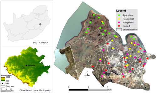
Our study area is located in the Emakhosaneni subplace (28°46′45.1″ S; 29°14′42.4″ E) in the central interior of the Okhahlamba Local Municipality in KwaZulu-Natal province, 17 km southwest of the town of Bergville (Figure 1). The area is located at an elevation of 1,150 m within a municipality that borders the Free State province and the Kingdom of Lesotho at the foothill of Drakensberg Mountain. It is a relatively humid area with strong seasonal rainfall patterns, receiving between 650 and 1200 mm of rainfall annually, most of it between October and March (Schulze et al. 1997). Average minimum temperatures are 12°C, and average maximum temperatures are 28 °C. Strong winds are typical of the area, especially during winter and spring months. The area is surrounded by various water sources, the Woodstock Dam to the north and the Tugela River and Driel dam to the east of the area. The area’s main geology comprises rock types of Triassic and Permian age, belonging to the Beaufort Group (Verster 1998). A total of 1,938 people lived in the area, covering 13.72 km², with an average density of 141.30 individuals per km² in 2011 (Statistics South Africa (SSA) 2011), which is expected to be slightly higher at present. The area is over 90% dominated by black Africans, who maintain a strong Zulu culture under traditional leadership. Large- and small-scale agricultural practices are dominated in this area, with stock grazing the grassland.

Figure 1. Location of the study area and distribution of the collected soil samples across main land use classes.

2.2. Soil sample collection

We first inspected the study area using high-resolution Google Earth (Google Earth 2020) and conducted a field campaign before identifying four main land-use classes occurring there, namely, agricultural land, residential land, eroded land, and rangeland. We collected a total of 52 soil samples, 13 from each category (their distribution is shown in Figure 1), from 16–19 July 2019. We selected samples based on a stratified random sampling strategy, a commonly used method to ensure that samples are representative of the area and eliminate any bias (Worsham et al. 2012). We collected samples from the soil surface to a depth of 15 cm using a standard auger with a dimension of 8 cm. We then placed the samples in a labelled, airtight plastic bag to prevent the sample from spilling or drying out, after which the GPS coordinates were recorded. At certain sampling points where the auger could not penetrate the soil surface, we used a spade, and the approximate volume of the sample was 750 cubic centimetres. We stored it in a cool and dry cooler box, away from direct sunlight and then in the laboratory for analysis.

2.3. Soil sample preparation

We dried about 500 g of each soil sample in the oven overnight at a temperature of 105 °C and after crushing the samples into fine soil particles using a porcelain mortar and pestle. We passed the crushed pieces through a 1 mm stainless steel sieve to ensure that large and foreign materials such as roots and stones are not included in the analysis and a more homogenous sample can be analysed. We then transferred the sieved samples to the respective labelled beakers and covered them with Parafilm M until analysis. The soil sample was separated into two parts for reflectance spectrum acquisition and for SOM determination. We used the Walkley-Black, one of the most common methods for determining the percentage of SOM content in soil samples (Motsara and Roy 2008). This is a wet oxidation method that uses acids to determine the amount of oxidizable carbon in the soil; this amount is then converted to SOM using a conversion factor (Walkley and Black 1934). For this study, we placed a small amount of the sieved soil sample in a conical flask together with potassium dichromate and sulphuric acid and left it for 30 min. After that, we added distilled water, orthophosphoric acid, and the indicator to the conical flask, which changed the colour of the solution to dark black. We titrated the solution in small increments against ferrous ammonium sulphate until the colour of the solution changed from black to green, indicating the endpoint of the titration. We then used the total volume of ferrous ammonium sulphate in the titration and recorded it while calculating the percentage of SOM content. We repeated this procedure for all soil samples.

2.4. Spectral data collection

A portable spectroradiometer known as the ASD FieldSpec3 (Analytical Spectral Devices Inc., Boulder, CO, USA) was used to collect the reflectance spectra of the soil samples in a dark laboratory environment under diffused light conditions. This instrument covers a spectral range from 350 nm to 2500 nm.

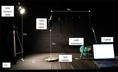
Approximately 500 g of oven-dried soil was placed in a black plastic dish that has a diameter of 22 cm and is 2 cm deep. A black plastic dish was used to ensure there was no interference from it during the collection of spectra. A study by Götze and Gläßer (2016) confirmed that black materials, such as plastic or rubber, have less than 8% reflectance over the range of 400-2400nm. The soil sample was then levelled to a smooth surface using a stainless-steel spatula. This step ensured a maximum diffuse reflection and a high signal-to-noise ratio during the collection of spectra (Mouazen et al. 2010). A smoother surface also reduces the amount of scattering. The plastic dish with the soil sample was then placed on a table with a black tablecloth for analysis. It is essential to ensure that the area of the black plastic dish is wider than the area covered by the ASD. Thus, Before the setup of the instrument, we calculated the estimated sample area of the fibre and the plastic dish using the following approach (Danner et al. 2015).

A 50 W halogen lamp (ASD; Analytical Spectral Devices, Inc.USA) was used as a source of illumination for the soil sample. The lamp was placed on a tripod and held 60 cm above the table at a 30° illumination zenith angle (Figure 2). A horizontal distance of 48 cm existed between the lamp and the centre of the soil sample. The pistol grip of the ASD FieldSpec3 spectroradiometer was also attached to a separate tripod and held 40 cm above the soil sample at a 0° zenith angle (i.e. it was pointed vertically towards the sample) (Figure 2a). The pistol grip contained a bare optic fibre which had a 25° field of view (FOV) and covered a circular area of 247.05 cm² was used to measure the spectral reflectance of the soil sample. Once the instrument was setup, the spectrometers and the lamp were warmed up for at least 2 h prior to starting the measurements. The spectral reflectance of the soil sample was measured using the inbuilt software (RS³, v6.3). A total of 10 reflectance spectra were then taken for the soil sample along 2151 bands (350–2500 nm), and the average was recorded as the reflectance spectrum for the soil sample. The above procedure was carried out for all 52 soil samples. The instrument was optimized every 30 min, and a white reference panel was collected every 15 min.

Figure 2. Overview of experimental setup.

2.5. Spectral data pre-processing

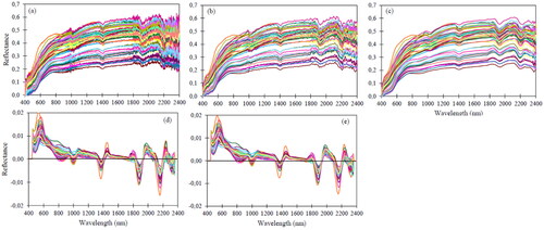
The raw spectra collected by the ASD instrument usually contain some noise (Figure 3a), and to reduce this noise, light scattering effects, and energy responses that varied along the different wavelengths, certain wavelengths were removed (Wang et al. 2017; Li et al. 2019). These wavelengths include the noisy ends of the beginning (350 nm to 399 nm) and ending regions (2401 nm to 2500 nm). This process reduced the number of bands from 2151 to 2001. Further, the remaining bands (ranging between 400 nm to 2400 nm) were then resampled using a 10 nm interval; this step further reduced the noise and the number of bands to 200 (Figure 3b). It also helped smooth the spectral curves that represented curve features such as absorption peaks and valleys of the soil samples. After resampling, the spectra were subjected to Savitzky–Golay (SG; Savitzky and Golay 1964) smoothing with a second-order polynomial with 11 smoothing points (five smoothing points on the left and five on the right) (Figure 3c). This method reduces the noise of spectra (e.g. baseline drift, tilt, reversal, etc.) and increases the signal-to-noise ratio while preserving the number of variables (Savitzky and Golay 1964). The SG smoothing method is defined in Equation (1)(1) $$\mathit{\text{Ai}},\mathit{\text{SG}}={\sum }_{i=\frac{1-m}{2}}^{\frac{m-1}{2}}{C}_j.A_i+j$$(1) . (1) $$\mathit{\text{Ai}},\mathit{\text{SG}}={\sum }_{i=\frac{1-m}{2}}^{\frac{m-1}{2}}{C}_j.A_i+j$$(1)

Figure 3. The reflectance curves showing the (a) raw spectra, (b) the reduced spectra, (c) the SG smoothened spectra, (d) the FDT transformed spectra of the soil samples, and (e) the combined pre-processed spectra (SG + FDT).

Where, $A_i,\mathit{\text{SG}}$ is the smoothed, and $A_i$ is the original reflectance value, $C_j$ is the filter coefficients, $j$ is the running index of the original data in the original data table, and $N$ is the number of convolution integers.

After the spectra were smoothed, we transformed them using the First-Order Derivative Transform with SG smoothing (FDT) (Figure 3d). This method helps correct baseline effects found in raw spectra and emphasizes small spectral variations that are not visible in the raw spectra (The Unscrambler 2014). These pre-treatment methods have often shown to be effective in similar studies as they smooth the spectra and reduce particle size effects and noise generated during the spectral data acquisition process (Vibhute et al. 2018). We then used the pre-processed spectra for further analysis, and we performed all pre-processing methods using the Unscrambler X software, version 10.4 (The Unscrambler 2014).

Finally, we averaged pre-processed spectra based on the different land use classes from which the soil samples were collected (i.e. agricultural, residential, eroded, and rangeland). We also obtained an overall average of all pre-processed spectra using the Unscrambler X software, and plotted the averaged spectra.

2.6. Spectral reflectance and analysis

We performed correlation analysis to examine the relationship between SOM content and soil samples’ reflectance, as Qiao et al. (2017) reported, as a reliable method for analysing the correlation between dependent and independent variables. The strength of the relationship between the two variables is expressed as a correlation coefficient (r) (Virgawati et al. 2019), which we calculated using Equation (2)(2) $$r=\frac{n(\sum \mathit{\text{xy}})-(\sum x)(\sum y)}{\sqrt{n(\sum x^2)-(\sum {x)}^2}\sqrt{n(\sum y^2)-(\sum {y)}^2}}$$(2) . (2) $$r=\frac{n(\sum \mathit{\text{xy}})-(\sum x)(\sum y)}{\sqrt{n(\sum x^2)-(\sum {x)}^2}\sqrt{n(\sum y^2)-(\sum {y)}^2}}$$(2)

Where, $n$ is the number of pairs of scores, x is the SOM content, y is the soil sample reflectance, $\sum \mathit{\text{xy}}$ is the sum of the products of paired scores, $\sum x$ is the sum of x scores, $\sum y$ is the sum of y scores, $\sum x^2$ is the sum of squared x scores, and $\sum y^2$ is the sum of squared y scores.

The correlation coefficient (r) value can range from +1 to −1. A value of 0 indicates that there is no relationship between the variables, while values closer to 1 or (–1) indicate a close positive or (negative) relationship. We calculated the correlation coefficient (r) values at each wavelength band from 400 nm to 2400 nm over the SOM content. We did this for both the raw and pre-processed spectra for the overall dataset and within each land use type using only the SG pre-processed data (agriculture, residential, eroded, and rangeland). We then plotted the correlation coefficient values, reiterating the procedure in the Unscrambler X software (The Unscrambler 2014).

2.6.1. Partial least squares regression

Partial Least Squares Regression (PLSR) is a widely used method to perform quantitative spectral data analysis (Rossel and Behrens 2010) and has proven to be a robust and reliable approach to quantitative spectral analysis. This is attributable to its ability to reduce dimensionality, synthesise, and solve collinearity problems between independent variables (Yu et al. 2016; Wang et al. 2017). The PLSR is similar to multiple linear regression, which relates the predictor (X) and response (Y) variables. However, it selects consecutive orthogonal factors, known as latent variables, that increase the covariance between the variables of the predictor (X-soil reflectance spectra) and the response variable (Y-SOM content). For more information on PLSR, we refer the reader to Martens and Naes (1989).

In this study, we performed a PLSR analysis to examine the relationship between SOM content and the collected reflectance spectra. We performed the analysis using the soil reflectance as a predictor variable and SOM content as a response variable. To determine the optimal number of latent variables for building the PLSR model, we used the leave-one-out cross-validation (LOOCV) method. This process minimises the overfitting or underfitting of data when building the PLSR model (Nawar et al. 2016). Furthermore, we averaged the data before applying a kernel PLS algorithm. Finally, we identified and removed outliers before proceeding with the analysis. We also performed the PLSR analysis using the Unscrambler X software.

2.6.2. PLSR model development and validation

Before the development of the PLSR models, we divided 52 sampling sites into two groups. The first group was the calibration samples used for creating the models (n = 36; 70% of sampling sites), while the second group was used for the validation of the models (n = 16; 30% of sampling sites). We created four PLSR models from the calibration dataset based on the following:

1. Raw spectra and SOM content (R)

2. Pre-processed SG spectra and SOM content (SG only)

3. Pre-processed FDT spectra and SOM content (FDT only)

4. Overall pre-processed spectra and SOM content (SG + FDT

We used the validation dataset to validate the accuracy of the PLSR prediction models. To test the prediction accuracy and strength of the PLSR models, we first calculated the coefficient of determination (R²) of the SOM predictions using Equation (3)(3) $$R^2=1-\frac{{\sum }_{i=1}^n(Y_{\mathit{\text{measured}}}-{Y_{\mathit{\text{predicted}}})}^2}{{\sum }_{i=1}^n(Y_{\mathit{\text{measured}}}-{Y_{\mathit{\text{mean}}})}^2}$$(3) . (3) $$R^2=1-\frac{{\sum }_{i=1}^n(Y_{\mathit{\text{measured}}}-{Y_{\mathit{\text{predicted}}})}^2}{{\sum }_{i=1}^n(Y_{\mathit{\text{measured}}}-{Y_{\mathit{\text{mean}}})}^2}$$(3)

Where, $Y_{\mathit{\text{measured}}}$ is the measured SOM content, $Y_{\mathit{\text{predicted}} }$ is the predicted SOM content, $Y_{\mathit{\text{mean}}}$ is the mean of the measured values, and $n$ is the number of samples.

Second, in order to test the accuracy of the different prediction methods used, we calculated the Root Mean Square Error (RMSE) for the calibration (RMSEC) and validation (RMSEP) datasets using Equations (4)(4) $$\mathit{\text{RMSEC}}=\sqrt{\frac{1}{N}} \sum _{i=1}^N{Y_m-Y}_c{)}^2$$(4) and (5)(5) $$\mathit{\text{RMSEP}}=\sqrt{\frac{1}{N}} \sum _{i=1}^N{Y_m-Y}_p{)}^2$$(5) . (4) $$\mathit{\text{RMSEC}}=\sqrt{\frac{1}{N}} \sum _{i=1}^N{Y_m-Y}_c{)}^2$$(4) (5) $$\mathit{\text{RMSEP}}=\sqrt{\frac{1}{N}} \sum _{i=1}^N{Y_m-Y}_p{)}^2$$(5)

Where $Y_m$ is the measured SOM content, $Y_c$ is the predicted SOM content derived from the calibration dataset,$Y_p$ is the predicted SOM content derived from the validation dataset, and $N$ is the number of samples.

3. Results

3.1. SOM analysis

Table 1 presents the descriptive statistics of SOM content collected over the main land use classes in the study area. Our results show that agricultural land use had the highest average SOM content (2.98%), minimum (1.87%) and maximum of (5.78%), while the rangeland class had the second highest average SOM content (2.46%) and minimum of (0.31%). Eroded and Residential classes had the average SOM content of (1.56%) and (1.77%), respectively. Relatively, rangeland class had the highest standard deviation (1.22), indicating an uneven spread of SOM content, while the residential class, on the other hand, had the lowest (0.91), with a more consistent SOM content. Overall, the average SOM content in the study area was 2.19% (Table 1).

Table 1. Descriptive statistics of the SOM within the study area’s main land use classes.

Land use	N	Mean (%)	Std. deviation (%)	Minimum (%)	Maximum (%)
Agriculture	13	2.98	1.14	1.87	5.78
Residential	13	1.77	0.91	0.78	3.90
Eroded	13	1.56	1.06	0.00	2.19
Rangeland	13	2.46	1.22	0.31	3.91
Overall	52	2.19	1.20	0.00	5.78

N: Number of samples; Std deviation: Standard deviation.

3.2. Spectral reflectance of soil samples

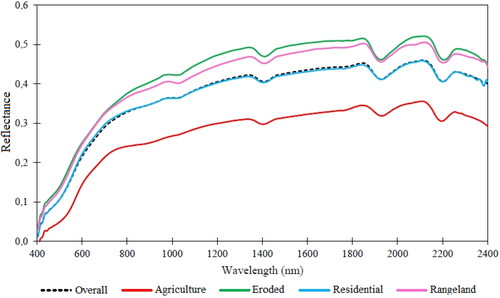
We plotted the average spectral reflectance curves of the soil samples in Figure 4. As can be seen in this figure, the spectral reflectance curves for the different land use classes exhibit a similar pattern across the spectrum range 400–2400 nm. All classes start at a relatively low reflectance at 400 nm, then increase exponentially to about 700 nm and further until they drop at 2400 nm. The average spectra for eroded class had the highest reflectance with the lowest in agriculture, while other classes are in-between. Remarkably, the eroded, rangeland, and residential are closely packed throughout the spectrum, above agriculture class.

Figure 4. The average spectral reflectance curves of soil samples obtained within each of the major land uses of the study area and the overall average spectral reflectance.

3.3. Relationship between SOM content and reflectance spectra

To better understand the relationship between SOM content and reflectance spectra, we plot the correlation coefficients (r), and the results are presented in Figure 5a–f, which show an apparent variability in the correlation coefficients across the (400–2400 nm) spectrum. Figure 5a,b, respectively show the overall correlation coefficients for the raw and pre-processed spectra (SG + FDT), and it is clear that after pre-processing, the curve is much smoother, especially at 1000–2400 nm, while the signatures differed. Figure 5a is predominantly in the –r starts, with a higher r = −0.19 at 400 nm and sharply drop to −0.38 in 600 nm, then increase from 800 nm, with clear peaks at 1400, 1900, and 2200 nm wavelengths. In Figure 5b traversed both negative and positive r, and starts around r = 0 and decrease in 550 nm, after which it fluctuates to a peak of >0.4 at 1400 nm, lowest r at 2000 nm and increase again thereafter. In Figure 5a, the highest (lowest) correlation coefficient was r= −0.19 in 400 nm (r= −0.39) in 700 nm), while in Figure 5b was r= −0.50 in 2004 nm, (r= −0.01) in 1774 nm.

Figure 5. Calculated correlation coefficients between SOM content and spectral reflectance of: (a) all raw spectra, (b) all pre-processed spectra, (c) SG pre-processed agriculture spectra, (d) SG pre-processed residential spectra, (e) SG pre-processed eroded spectra, and (f) SG pre-processed rangeland spectra.

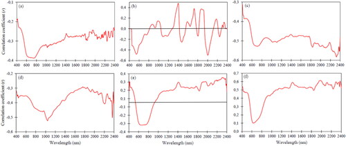
The spectral signature in Figures 5c–f also shows a behaviour to that of the raw overall correlation coefficient curve (Figure 5a). The correlation coefficient curves for the different land uses showed smoother curves but with different coefficient values. In Figure 5c, the shape of the curve is similar to that of the raw curve shown in Figure 5a, but up to 1800 nm. The curve starts high at 400 nm and then slopes down to around 600 nm to 800 nm, after which it until it reaches 1800 nm, then coefficient values seem to be decreasing until 2400 nm. The correlation coefficients for the agriculture land use were also negative, with the highest correlation coefficient around 400 nm (r= −0.31) and the lowest correlation coefficient at 2324 nm (r= −0.58). Subsequently, in Figure 5d, it can be seen that there is a slight decrease in coefficient values along the 400 nm region, followed by an increase from 450 nm to 600 nm and a slight decrease thereafter to 964 nm.

The SG smoothing method greatly facilitated the removal of noise caused by the instrument or other factors. We notice more fluctuations across the spectrum than the raw spectral curve (Figure 5a), probably due to the FDT method used during the pre-treatment process of the raw spectra. With reference to the raw spectra curve, the correlation coefficients in the VIS region (400–700 nm) were higher than in the NIR region (700–2400 nm). VIS reflects in soil colour, and the absorption bands in this region are largely influenced by the SOM content and may have resulted in higher correlation values than the NIR region (Duarte and Duarte 2019). As already stated, the water absorption bands (1400 nm and 1900 nm) and 2200 nm had high absorption, here the correlation coefficients were highest in the NIR region (Figure 5a), suggesting a relationship between the SOM content and the absorption in these bands.

Our results show that the correlation coefficients were not high; they were all negative (Figure 5a), indicating a weakly negative relationship between the SOM content and the spectral reflectance of the collected soil samples. On the other hand, the pre-processed curve had higher correlation coefficients in the NIR region compared to the VIS region, probably because of the FDT method, which according to Kooistra et al. (2001), generally has little influence on the VIS region and the beginning of the NIR region, since the absorption features are rather broad in these regions. This consideration may also account for the shape of the curve in these regions compared to the rest of the NIR region, where distinct peaks and minima drops correlation coefficients are located. Subsequently, the FDT method removes the baseline from the spectra whilst emphasizing absorption features (Buddenbaum and Steffens 2012). The NIR region consists of absorption peaks that have now become amplified due to the applied pre-processing methods. This could have influenced the higher correlation coefficients observed in this region, especially at 1404 nm and 2004 nm (Figure 5b). The results in Figure 5b were improved after the pre-processing the spectra as shown in Figure 5, suggesting a moderate relationship between the analyzed SOM content and the pre-processed spectral reflectance of the soil samples. These results agree with Gao et al. (2017), Hong et al. (2018a), and Wei et al. (2020), where negative correlations were also seen between SOM content and spectral reflectance for the overall raw and pre-processed spectra.

Additionally, the correlation coefficients obtained from the different land use types only focused on the relationship between pre-processed reflectance spectra using the SG method and the SOM content. Correlation coefficients curves varied along the across the wavelength range for each of the land use class, where all the land use classes showed a similar trend in correlation values in the VIS region except for the residential (Figure 5d). Note that soil samples obtained from this class had variations in soil colour. This variation, coupled with the relatively low SOM content within this land use type, may have influenced the spectral reflectance, thus resulting in the moderately weak correlation along this region. In contrast, the correlation coefficients in the NIR region were higher for all the land use types, with the exception of the agriculture class (Figures 5c–f). This may be attributed to the fact that agriculture had the highest SOM content and that its reflectance was influenced by this, resulting in weak correlations along this region. According to Virgawati et al. (2019), this indicates that SOM and reflectance of soil samples have ‘negative associations with strong relationships’. This, coupled with the number of absorption bands in the NIR region, may have caused the higher correlation values. Furthermore, correlations were negative for the agriculture, and residential land uses, positive for the rangeland land use, and a combination of both for the eroded land. Therefore, indicating that agriculture SOM content had a negatively moderate to strong correlation with its reflectance spectra, residential class had a similar trend, eroded class had a moderately positive correlation with its reflectance spectra, and rangeland land use positively correlated with its reflectance spectra. It also suggests that an increase in SOM content will result in a decreased reflectance of the soil samples and that the converse relationship will be seen as SOM content decreases.

3.4. PLSR modelling analysis

In Table 2, we displayed the results of the performance of the different PLSR models created using both raw spectral data and different pre-processing methods. With regards to the R² values, for the calibration dataset, values range from 0.28 (lowest) to 0.49 (highest), while the validation dataset values range from 0.22 (lowest) to 0.34 (highest). However, in terms of the RMSE, the error values were higher than that of the R² values. For the calibration dataset, RMSEC values ranged from 0.73% to 0.98%, while in the validation dataset, RMSEP values ranged from 1.08% to 1.11%. Regarding each of the PLSR models, the R and SG models had similar results where both their R² and RMSE values were quite similar with little to no difference. However, the FDT and SG + FDT models had higher R² values with lower RMSE values in the calibration dataset compared to the validation dataset where the converse trend was seen. Subsequently, the FDT model has the highest R² value (0.49) and lowest RMSEC value (0.73%) in the calibration dataset, but in the validation dataset, it had the lowest R² value (0.22) and the highest RMSEP value (1.11%). A similar but contrasting trend can also be seen for the SG model, while the R and SG + FDT models have values and trends that fall in between the other PLSR models.

Table 2. The statistical summary of the different PLSR models created using raw and different pre-processed spectral data and SOM content.

PLSR model type	Calibration		Validation
	R^2	RMSEC (%)	R^2	RMSEP (%)
R	0.31	0.95	0.33	1.08
SG	0.28	0.98	0.34	1.08
FDT	0.49	0.73	0.22	1.11
SG + FDT	0.46	0.75	0.25	1.09

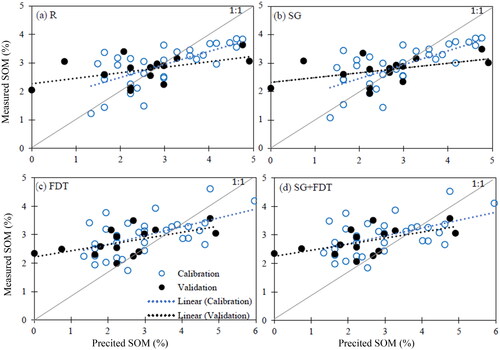
In Figure 6, we plotted the measured SOM content against the predicted SOM content derived from the PLSR models. Our results show a relatively constant pattern with the lines of best fit. In particular, Figure 6a, show most randomly distributed data points in close to their respective best fit lines for both the calibration and validation datasets. The SG plot (Figure 6b) is quite similar to that of the R plot (Figure 6a), except for few points having slightly different values. In Figure 6c, data points are more compact and closer to their respective lines of best fit for both the calibration and validation datasets. Figure 6d show a similar confirmation to that of Figure 6c, except for slight variation of values.

Figure 6. Scatterplots of measured versus predicted SOM content using the four derived PLSR models: (a) R, (b) SG, (c) FDT and (d) SG + FDT.

4. Discussion

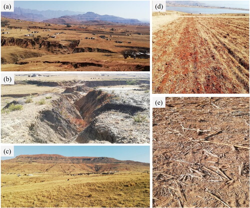
In this study, we examined soil organic matter and its relationship to spectroscopy data. To achieve this, we compared the accuracy of PLSR models derived from the use of raw spectral data and various pre-processing methods against measured SOM content. Our results showed that the average SOM content of the area is 2.19%, with agricultural land (2.98%) and rangeland (2.46%) having an average SOM content slightly higher than that of the area. Both the residential (1.77%) and the eroded land area (1.56%) were below the average SOM content of the area. Several small-scale farms exist in the area, and play key role in the formation and maintenance of SOM content. For example, crops are regularly grown on agricultural areas, so there is a regular supply of organic matter in the form of leaf litter and stems (see Figure 7e) added to the soil (Behera and Prasad, 2020). Additionally, soils in agricultural landscapes are typically maintained regularly through irrigation and manure application to higher crop yields (see Fig, 7d), which adds in the enrichment of SOM content (Bot and Benites 2005). In part, rangeland could also have contributed to a higher proportion of SOM, as it is often extensive vegetation animal manure from livestock grazing (see Figure 7c) and can influence SOM content in the region (Haynes et al. 2003). The central to eastern regions of the study are subject to severe erosion (Figure 7(a,b)), which may explain the lower percentages of SOM content. Phuong and Son (2017) noted that SOM and rich topsoil are lost as a result of soil erosion. In their SOM prediction over a mountainous region in China, Liu et al. (2015) observed high spatial variability in various land-use classes. However, the average reflectance of the spectra showed an inverse pattern, being higher on eroded areas and decreasing to a minimum on agricultural areas.

Figure 7. Landscape conditions in the study area; (a,b) severe erosion problem in the Central and Eastern parts, (c) rangeland in the Central Eastern parts, (d) agricultural areas in the fallow time, (e) and maize crop residues dispersed in the farm.

The results of our PLSR model showed different performances, which is consistent with Vibhute et al. (2018), where the soil reflectance spectra can explain the SOM content. The R model achieved a relatively higher R² value for calibration (0.31) and validation (0.33) of the raw spectra and measured SOM content, with the RMSE values of 0.95 and 1.08, respectively. Previous studies (Gao et al. 2017; Wang et al. 2017; Li et al. 2019) showed raw spectra to be contaminated by instrument noise, light scattering effects, or energy responses that vary along the different wavelengths. This could have affected the performance of the R model and thus its R² values. The problem of overfitting or underfitting the PLSR model is common in such studies (Castillo et al. 2005). In our case, however, the error for the validation dataset is larger than that for the calibration dataset, suggesting that the overfitting was quite small. Our results are comparable to Bangelesa et al. (2020). The SG model yielded the lowest (0.28) and highest (0.34) R² values, while the calibration and validation dataset had the highest (0.98) and lowest (1.08) RMSE values, respectively. This means that the SG model was responsible for 28% of the variability in SOM content in the calibration dataset and 34% of the SOM content in the validation dataset. The slight improvement in the R² value of the SG model is directly attributable to the fact that the spectra used to create the PLSR model were pre-processed using the SG method. This pre-processing method is often used in spectral analysis to remove inappropriate information that may be present in the spectral data (Gholizadeh et al. 2013). The SG method is also used to reduce any noise that may be present (e.g. baseline drift) which may be present in the spectra and to increase the signal-to-noise ratio (Savitzky and Golay 1964). Removing the noise from the raw spectra eliminated any unnecessary information and/or inconsistencies that may have been present therein. According to Vasques et al. (2008), the SG smoothing method is a common pre-treatment method for improving SOM model results. This observation is reflected in our results.

The FDT model outperformed all PLSR models on the calibration dataset, achieving the highest R² (0.49) and the lowest RMSE (0.73). In contrast, it achieved the lowest R² value (0.22) and the highest RMSE (1.11) for the validation dataset than all PLSR models. Thus, the FDT model explained 49% and 22% of the variability in SOM content for the calibration dataset and the validation dataset, respectively. FDT is a transformation method that helps in correcting baseline effects in raw spectra and is useful for smoothing, removing noise and reducing particle size effects in raw spectra (Bilgili et al. 2010; Srivastava et al. 2017; Vibhute et al. 2018). According to Fang et al. (2018), performing the FDT method can amplify the noise present in the spectral data. Finally, SG + FDT was the second best PLSR model, that accounted for 46% of the variability of SOM content in the calibration dataset and 25% of the variability of SOM content in the validation dataset. This model had an RMSE of 0.75 for the calibration dataset and 1.09 for the validation. Here, both pre-processing methods were used, with the SG method being applied to the raw spectra, and then the FDT method being applied to the SG pre-processed spectra. By combining the two pre-processing methods, the results of the model were improved. As reported by Li et al. (2015), the combination of SG smoothing and FDT has shown to be superior in improving PLSR models. Since this model used two pre-processing methods, its results are also influenced by the aforementioned assertation. For example, when the SG method was performed on the raw spectra, some of the noise may not have been completely removed, and when the FDT was performed on this data, present noise may have been amplified, thus causing the model performance to decrease while the error increases.

Though, the results of the calibration dataset seem to be better than those of the validation dataset, the model cannot work in any application due to very low R² (<0.60) (Williams et al. 2019). This observation is explained by Kuang and Mouazen (2012) that increasing the number of samples improves the accuracy of the prediction and its RMSEP. Because of the calibration dataset had a larger number of samples than the validation dataset, its performance was greater. Furthermore, the results of these datasets showed that the calibration dataset had higher R² values with lower RMSEC values, while the validation dataset showed the opposite behaviour. Similar to Shepherd and Walsh (2002) and Kuang and Mouazen (2012), R² values increased, and the RMSE for the calibration dataset decreased due to a larger number of samples were used in the calibration dataset than in the validation dataset. As a result, the PLSR method itself and the way it calculates the predicted values could also have affected the values of the evaluation statistics.

Our analysis highlights the value of PLSR models for predicting SOM content using spectral data, with pre-processing methods generally outperforming the model based on raw spectra. Specifically, the FDT-PLSR model produced the most accurate model results, followed by the SG + FDT model, the SG model, with the R model being the least. Our results are consistent with Kuang and Mouazen (2012); Nawar et al. (2016); Wang et al. (2017); Šestak et al. (2018); Vibhute et al. (2018); Bangelesa et al. (2020), who also found an increase in the prediction accuracy of SOM content using pre-processed reflectance spectral. Overall, the R and SG models appear to perform worse in predicting SOM content than the FDT and SG + FDT models, which achieved better prediction of SOM content.

5. Conclusion

In this study, we analyse the relationship between the SOM and the spectral reflectance of soils collected in the agricultural, residential, rangeland and eroded classes in the Emakhosaneni area, South Africa. Our results show that as the SOM content in a soil sample increases, the spectral reflectivity decreases for more absorption due to higher hydrogen bonds content in soil. This pattern was particularly observed in the agricultural and eroded classes with the highest and lowest SOM content, respectively. The correlation coefficients between negative and moderately strong relationship between SOM content and spectral reflectance over the entire wavelength range sampled. Our PLSR showed that the pre-processed data models performed better than that of the raw spectral data. The different pre-processing methods treated spectral noise, baseline offset, and absorption differently in the spectral data and also revealed their importance and influence on the performance and accuracy of the PLSR models. Based on our results, we conclude that pre-treatment with the FDT method produces a positive response on the performance of the PLSR model in predicting SOM content. Despite the low performance of these models, they emphasized the importance of VNIR spectroscopy in measuring and predicting SOM content compared to traditional laboratory methods, which can be time-consuming and costly. Since SOM content determines the biophysical and chemical properties of soil, it is essential to properly manage SOM content and soils to achieve sustainable goals in agriculture and land management. Our results confirm previous studies, and we encourage further studies in different seasons and landscapes.

Disclosure statement

No potential conflict of interest was reported by the author(s).

References

- Adeline KR, Gomez C, Gorretta N, Roger JM. 2017. Predictive ability of soil properties to spectral degradation from laboratory Vis-NIR spectroscopy data. Geoderma. 288:143–153. doi: 10.1016/j.geoderma.2016.11.010.
- Angelopoulou T, Balafoutis A, Zalidis G, Bochtis D. 2020. From laboratory to proximal sensing spectroscopy for soil organic carbon estimation—A review. Sustainability. 12(2):443. doi: 10.3390/su12020443.
- Ayala Izurieta JE, Jara Santillán CA, Márquez CO, García VJ, Rivera-Caicedo JP, Van Wittenberghe S, Delegido J, Verrelst J. 2022. Improving the remote estimation of soil organic carbon in complex ecosystems with Sentinel-2 and GIS using Gaussian processes regression. Plant Soil. 479(1-2):159–183. doi: 10.1007/s11104-022-05506-1.
- Bangelesa F, Adam E, Knight J, Dhau I, Ramudzuli M, Mokotjomela TM. 2020. Predicting soil organic carbon content using hyperspectral remote sensing in a degraded mountain landscape in Lesotho. Appl Environ Soil Sci. 2020:2158573.
- Behera BK, Prasad R. 2020. Environmental technology and sustainability: physical, chemical and biological technologies for clean environmental management. The Netherlands: Elsevier.
- Bernini A, Bosino A, Botha GA, Maerker M. 2021. Evaluation of gully erosion susceptibility using a maximum entropy model in the Upper Mkhomazi River Basin in South Africa. ISPRS Int. J. Geoinf. 10:729.
- Bilgili AV, Van Es HM, Akbas F, Durak A, Hively WD. 2010. Visible-near infrared reflectance spectroscopy for assessment of soil properties in a semi-arid area of Turkey. J Arid Environ. 74:229–238.
- Bot A, Benites J. 2005. The importance of soil organic matter: key to drought-resistant soil and sustained food production; FAO Soils Bulletin 80; Food and Agricultural Organization of the United Nations, Rome, Italy.
- Buddenbaum H, Steffens M. 2012. The effects of spectral pretreatments on chemometric analyses of soil profiles using laboratory imaging spectroscopy. Appl. Environ. Soil Sci. 2012:1–12. doi: 10.1155/2012/274903.
- Castillo E, Iglesias A, Ruiz-Cobo R. 2005. Chapter 9- Functional networks. Functional equations in applied sciences. 169–232.
- Danner M, Locherer M, Hank T, Richter K. 2015. Spectral sampling with the ASD FieldSpec 4–theory, measurement, problems, interpretation. EnMAP Field Guides Technical Report, GFZ Data Services, Potsdam, Germany, 1–25.
- Du Preez CC, Van Huyssteen CW, Mnkeni PN. 2011. Land use and soil organic matter in South Africa 2: a review on the influence of arable crop production. S Afr J Sci. 107(5/6):1–8. doi: 10.4102/sajs.v107i5/6.358.
- Duarte RMBO, Duarte AC. 2019. Geochemistry soil, organic components. In Worsfold P, Poole C, Townshend A, Miró M, editors. Encyclopedia of analytical science. 3rd ed. Oxford: Academic Press; p. 329–339.
- Fang Q, Hong H, Zhao L, Kukolich S, Yin K, Wang C. 2018. Visible and near-infrared reflectance spectroscopy for investigating soil mineralogy: a review. J Spectrosc. 2018:1–14.
- Gao L, Zhu X, Han Z, Wang L, Zhao G, Jiang Y. 2017. Spectroscopy based estimation of soil organic matter in Brown-Forest areas of the Shandong Peninsula, China. Pedosphere. 1–12.
- Gholizadeh A, Borůvka L, Saberioon M, Vašát R. 2013. Visible, near-infrared, and mid-infrared spectroscopy applications for soil assessment with emphasis on soil organic matter content and quality: state-of-the-art and key issues. Appl Spectrosc. 67(12):1349–1362. doi: 10.1366/13-07288.
- Google Earth. 2020. Emakhosaneni area. [accessed 2020 May 12]. https://earth.google.com/web/@-28.79943144,29.23423194,1272.68696279a,3832.42087508d,35y,0h,0t,0r/data=ChUaEwoLL2cvMXRkM2NmYnQYAiABKAI.
- Götze C, Gläßer C. 2016. Spectral characterization of black materials for use as background in spectrometric laboratories. Spectrosc Lett. 49(7):498–505. doi: 10.1080/00387010.2016.1211708.
- Haynes RJ, Dominy CS, Graham MH. 2003. Effect of agricultural land use on soil organic matter status and the composition of earthworm communities in KwaZulu-Natal, South Africa. Agric Ecosyst Environ. 95:453–464.
- He T, Wang J, Lin Z, Cheng Y. 2009. Spectral features of soil organic matter. Geo Spat Inf Sci. 12:33–40.
- Hong Y, Chen S, Liu Y, Zhang Y, Yu L, Chen Y, Liu Y, Cheng H, Liu Y. 2019. Combination of fractional order derivative and memory-based learning algorithm to improve the estimation accuracy of soil organic matter by visible and near-infrared spectroscopy. Catena. 174:104–116. doi: 10.1016/j.catena.2018.10.051.
- Hong Y, Chen S, Zhang Y, Chen Y, Yu L, Liu Y, Liu Y, Cheng H, Liu Y. 2018a. Rapid identification of soil organic matter level via visible and near-infrared spectroscopy: effects of two-dimensional correlation coefficient and extreme learning machine. Sci. Total Environ. 644:1232–1243. doi: 10.1016/j.scitotenv.2018.06.319.
- Hong Y, Yu L, Chen Y, Liu Y, Liu Y, Liu Y, Cheng H. 2018b. Prediction of soil organic matter by VIS–NIR spectroscopy using normalized soil moisture index as a proxy of soil moisture. Remote Sens. 10:28.
- Jia X, Xie M, Hu B, Zhou Y, Li H, Zhao W, Deng W, Shi Z. 2023. Prediction of soil organic carbon contents in Tibet using a visible near-infrared spectral library. Eurasian Soil Sci. 56:727–737.
- Kooistra L, Wehrens R, Leuven RSEW, Buydens LMC. 2001. Possibilities of visible–near-infrared spectroscopy for the assessment of soil contamination in river floodplains. Anal. Chim. Acta. 446(1-2):97–105. doi: 10.1016/S0003-2670(01)01265-X.
- Kuang B, Mouazen AM. 2012. Influence of the number of samples on prediction error of visible and near infrared spectroscopy of selected soil properties at the farm scale. Eur. J. Soil Sci. 63:421–429.
- Li S, Shi Z, Chen S, Ji W, Zhou L, Yu W, Webster R. 2015. In situ measurements of organic carbon in soil profiles using vis-NIR spectroscopy on the Qinghai–Tibet plateau. Environ Sci Technol. 49(8):4980–4987.
- Li X, Ren J, Zhao K, Liang Z. 2019. Correlation between spectral characteristics and physicochemical parameters of soda-saline soils in different states. Remote Sens. 11:388.
- Liu H, Zhang Y, Zhang B. 2009. Novel hyperspectral reflectance models for estimating black-soil organic matter in Northeast China. Environ Monit Assess. 154(1-4):147–154. doi: 10.1007/s10661-008-0385-4.
- Luo C, Zhang X, Meng X, Zhu H, Ni C, Chen M, Liu H. 2022. Regional mapping of soil organic matter content using multitemporal synthetic Landsat 8 images in Google Earth Engine. Catena. 209:105842. doi: 10.1016/j.catena.2021.105842.
- Martens H, Naes T. 1989. Assessment, validation and choice of calibration method. In Multivariate calibration. 1st ed. New York: John Wiley & Sons; p. 237–266.
- Mchunu C, Chaplot V. 2012. Land degradation impact on soil carbon losses through water erosion and CO2 emissions. Geoderma. 177-178:72–79. doi: 10.1016/j.geoderma.2012.01.038.
- Motsara MR, Roy RN. 2008. Guide to laboratory establishment for plant nutrient analysis. In FAO fertilizer and plant nutrition bulletin. Rome: Food and Agriculture Organization; p. 1–219.
- Mouazen AM, Kuang B, De Baerdemaeker J, Ramon H. 2010. Comparison among principal component, partial least squares and back propagation neural network analyses for accuracy of measurement of selected soil properties with visible and near infrared spectroscopy. Geoderma. 158(1-2):23–31. doi: 10.1016/j.geoderma.2010.03.001.
- Nawar S, Buddenbaum H, Hill J, Kozak J, Mouazen AM. 2016. Estimating the soil clay content and organic matter by means of different calibration methods of vis-NIR diffuse reflectance spectroscopy. Soil Tillage Res. 155:510–522. doi: 10.1016/j.still.2015.07.021.
- Obalum SE, Chibuike GU, Peth S, Ouyang Y. 2017. Soil organic matter as sole indicator of soil degradation. Environ Monit Assess. 189(4):176. doi: 10.1007/s10661-017-5881-y.
- Phuong TT, Son NT. 2017. Land use change and its interactions with soil, water resources, and rural livelihoods in Hoa Binh province. Vietnam J Agric Sci. 15:249–262.
- Qiao XX, Wang C, Feng MC, Yang WD, Ding GW, Sun H, Liang ZY, Shi CC. 2017. Hyperspectral estimation of soil organic matter based on different spectral preprocessing techniques. Spectrosc. Lett. 50(3):156–163. doi: 10.1080/00387010.2017.1297958.
- Roper WR, Robarge WP, Osmond DL, Heitman JL. 2019. Comparing four methods of measuring soil organic matter in North Carolina soils. Soil Sci. Soc. Am. J. 83:466–474.
- Rossel RV, Behrens T. 2010. Using data mining to model and interpret soil diffuse reflectance spectra. Geoderma. 158(1-2):46–54. doi: 10.1016/j.geoderma.2009.12.025.
- Rossel RV, Walvoort DJJ, McBratney AB, Janik LJ, Skjemstad JO. 2006. Visible, near infrared, mid infrared or combined diffuse reflectance spectroscopy for simultaneous assessment of various soil properties. Geoderma. 131(1-2):59–75. doi: 10.1016/j.geoderma.2005.03.007.
- Roudier P, Hedley CB, Lobsey CR, Rossel RV, Leroux C. 2017. Evaluation of two methods to eliminate the effect of water from soil vis–NIR spectra for predictions of organic carbon. Geoderma. 296:98–107. doi: 10.1016/j.geoderma.2017.02.014.
- Santoiemma G. 2018. Recent methodologies for studying the soil organic matter. Appl Soil Ecol. 123:546–550. doi: 10.1016/j.apsoil.2017.09.011.
- Savitzky A, Golay MJ. 1964. Smoothing and differentiation of data by simplified least squares procedures. Anal Chem. 36(8):1627–1639. doi: 10.1021/ac60214a047.
- Schulze R, Maharaj M, Lynch SD, Howe BJ, Melvil-Thomson B. 1997. South African atlas of agrohydrology and climatology. Water Research Commission Report TT82/96, University of Natal, Pietermaritzburg, South Africa.
- Shepherd KD, Walsh MG. 2002. Development of reflectance spectral libraries for characterization of soil properties. Soil Sci Soc Am J. 66(3):988–998. doi: 10.2136/sssaj2002.0988.
- Srivastava R, Sethi M, Yadav RK, Bundela DS, Singh M, Chattaraj S, Singh SK, Nasre RA, Bishnoi SR, Dhale S, et al. 2017. Visible-near infrared reflectance spectroscopy for rapid characterization of salt-affected soil in the Indo-Gangetic Plains of Haryana, India. J Indian Soc Remote Sens. 45(2):307–315. doi: 10.1007/s12524-016-0587-0.
- Statistics South Africa (SSA). 2011. Census 2011. [accessed 2019 June 20]. http://www.statssa.gov.za/.
- The Unscrambler. 2014. The Unscrambler X v10.3 user manual. CAMO software AS, Nedre Vollgate, Oslo, Norway, 1–1370.
- Van der Meer F. 2018. Near-infrared laboratory spectroscopy of mineral chemistry: a review. Int. J. Appl. Earth Obs. Geoinf. 65:71–78. doi: 10.1016/j.jag.2017.10.004.
- Vasques GM, Grunwald SJOS, Sickman JO. 2008. Comparison of multivariate methods for inferential modeling of soil carbon using visible/near-infrared spectra. Geoderma. 146(1-2):14–25. doi: 10.1016/j.geoderma.2008.04.007.
- Verster PSJ. 1998. Geological map 2828 (Harrismith), 1:250 000. Council for Geoscience, Pretoria, South Africa.
- Vibhute AD, Kale KV, Mehrotra SC, Dhumal RK, Nagne AD. 2018. Determination of soil physicochemical attributes in farming sites through visible, near-infrared diffuse reflectance spectroscopy and PLSR modeling. Ecol Process. 7(1):1–12. doi: 10.1186/s13717-018-0138-4.
- Virgawati S, Mawardi M, Sutiarso L, Shibusawa S, Segah H, Kodaira M. 2019. Explore the character of soil spectral reflectance relate to the soil organic matter content. J. Tek. Pertanian Lampung. 8:214–223.
- Walkley A, Black IA. 1934. An examination of the Degtjareff method for determining soil organic matter, and a proposed modification of the chromic acid titration method. Soil Sci. 37(1):29–38. doi: 10.1097/00010694-193401000-00003.
- Wang J, Tiyip T, Ding J, Zhang D, Liu W, Wang F. 2017. Quantitative estimation of organic matter content in arid soil using Vis-NIR spectroscopy preprocessed by fractional derivative. J. Spectrosc. 2017:1–9.
- Wei L, Yuan Z, Wang Z, Zhao L, Zhang Y, Lu X, Cao L. 2020. Hyperspectral inversion of soil organic matter content based on a combined spectral index model. Sensors. 20(10):2777. doi: 10.3390/s20102777.
- Williams P, Manley M, Antoniszyn J. 2019. Near infrared technology: getting the best out of light. African Sun Media.
- Worsham L, Markewitz D, Nibbelink NP, West LT. 2012. A comparison of three field sampling methods to estimate soil carbon content. For. Sci. 58:513–522.
- Yu X, Liu Q, Wang Y, Liu X, Liu X. 2016. Evaluation of MLSR and PLSR for estimating soil element contents using visible/near-infrared spectroscopy in apple orchards on the Jiaodong peninsula. Catena. 137:340–349. doi: 10.1016/j.catena.2015.09.024.
- Zhao Y, Wang X, Chen F, Li J, Wu J, Sun Y, Zhang Y, Deng T, Jiang S, Zhou X, et al. 2023. Soil organic matter enhances aboveground biomass in alpine grassland under drought. Geoderma. 433:116430. doi: 10.1016/j.geoderma.2023.116430.