Cropping intensity mapping in Sentinel-2 and Landsat-8/9 remote sensing data using temporal transfer of a stacked ensemble machine learning model within google earth engine

Abstract

This article aimed to map Cropping Intensity Patterns (CIPs) in the southwest region of Iran using Google Earth Engine and monthly composites of Sentinel-2 and Landsat-8/9 data. To detect CIPs with high inter- and intra-class variability of crops, a heterogeneous Stack ensemble of machine learning model was developed. The model incorporated the Minimum Distance (MD) approach as a meta-classifier, combining multiple base models, including Support Vector Machines (SVM), Random Forest (RF), Classification and Regression Trees (CART), and Gradient Boosted Trees (GBT). In 2021, the Stack model was trained and evaluated using Ground Truth (GT) samples from the same year, achieving an Overall Accuracy (OA) of 94.24%. This performance surpassed the base models by about 4% in OA and was also reflected in the detection accuracies, including User’s Accuracy (UA), Producer’s Accuracy (PA), and F1-score, of the target classes. Subsequently, the trained stack model was temporally transferred to generate CIP maps for other years. The model achieved high OAs of 91.82% and 90.97% based on GT samples from 2020 and 2022, respectively. Finally, the time series of CIP maps (2019-2023) were utilized by the Cellular Automata-Markov model to forecast the map for 2024.

Keywords:

• Remote sensing
• cropping intensity patterns
• ensemble machine learning
• optical satellite data
• google earth engine

1. Introduction

The world’s population is growing rapidly, and the effects of climate change are putting pressure on farmers to increase crop production on arable lands (Smith 2013; MohanRajan et al. 2020; Shibabaw et al. 2023). Cropping Intensity Patterns (CIPs) are used to determine how many crops are grown on a particular farm during a Cropping Year (CY) (Liu et al. 2020). There are two main types of CIPs: mono-cropping and double-cropping (Zhao et al. 2021). Mono-cropping involves growing a single crop on a farm in a CY, either in autumn or in spring. In contrast, double-cropping involves growing two crops in succession on the same land in a CY, one in autumn and one in spring. The different CIPs have different environmental impacts, such as water usage, nutrient requirements, and greenhouse gas emissions. This is due to the different methods used for drainage, irrigation, and fertilization of each CIP (Zhang et al. 2021).

Accurate mapping of the spatial distribution of CIPs is essential to evaluate their ecological impact and promote sustainable land management practices. Moreover, CIP maps can be used as a basis for crop type classification (Wu et al. 2018), providing decision-makers with a clear view of the area allocated to autumn and spring crops. This can be particularly useful in ensuring food security for societies (Liu et al. 2020; You and Sun 2022). Therefore, it is crucial to map different CIPs accurately and continuously monitor their changes over time. The traditional methods of obtaining CIPs through field surveys and censuses can be costly, and time-consuming, and may provide limited and incomplete data (Ghosh et al. 2023). Remote Sensing (RS) satellite data has emerged as a valuable alternative for generating accurate, up-to-date, and detailed CIP maps by providing many advantages such as revisit capabilities, rich spectral information, promising spatial resolutions, and long historical records (Sishodia et al. 2020; You and Sun 2022).

Traditionally, low spatial resolution (≥250 m) satellite images with short revisit cycles, such as Moderate Resolution Imaging Spectroradiometer (MODIS), have been used to generate agricultural classification maps of various target classes to monitor land cover changes (Gray et al. 2014; Ghaderpour et al. 2023; Shawky et al. 2023). However, due to their coarse spatial resolution, the phenomenon of mixed pixels occurs, making it difficult to identify CIPs accurately (Lobell and Asner 2004). Medium-resolution images like Sentinel-2 (S2) and Landsat-8/9 (L8/9) are better suited for agricultural applications as they provide more detailed spatial information and help mitigate the issue of mixed pixels (Khanal et al. 2020).

Most studies reviewed in the literature utilized multi-temporal RS data to cover the entire CY for generating agricultural-related maps (Pluto-Kossakowska 2021). This approach allows for a comprehensive understanding of phenological changes occurring throughout the growing season, facilitating the accurate identification of different CIPs. Likewise, most studies mainly utilized a single source of RS data, either S2 or L8/9 (Rahmati et al. 2022; Mullapudi et al. 2023). However, combining these two data sources can enhance the density of cloud-free observations, as each satellite acquires data at different times (Shen et al. 2023). By synergistically using S2 and L8/9, it is also possible to generate detailed phenological time series, resulting in improved classification accuracy of CIPs since the temporal changes in agricultural lands can be more effectively observed (Gao et al. 2023).

The use of multi-temporal and multi-source approaches for RS applications can pose significant challenges due to the vast amount of data that needs to be stored and processed (Taheri Dehkordi et al. 2022). However, in recent years, the emergence of GEE has simplified RS applications by providing a cloud-based processing platform (Gorelick et al. 2017). GEE has been widely used in various fields, such as water resources management (Taheri Dehkordi et al. 2022), long-term land cover change detection (Sidhu et al. 2018), and land cover classification (Huang et al. 2017). With GEE, users can easily access Java and Python Application Programming Interfaces (APIs), which eliminates the need to download data for different tasks. This allows for the development of innovative classification approaches with enhanced accuracy using GEE's capabilities. As a result, scientists can obtain more accurate results in near real-time earth observation applications of RS data (Abdali et al. 2023).

Previous studies on mapping CIPs have used either phenology-based or traditional peak extractor methods (Guo et al. 2022). However, these methods have limitations due to variations in crop types and climate conditions that can cause significant changes in the duration of the crop growth cycle. In addition, peak extractor methods are susceptible to errors and uncertainties, making it necessary to employ multiple constraints to eliminate fake peaks (Xiang et al. 2019). These methods also disregard in-situ knowledge about crop phenology and intensity, leading to challenges in mapping CIPs across extensive spatial areas and multiple years (Yan et al. 2019; Guo et al. 2022).

To address these challenges, a classification approach that can effectively handle the high variabilities of crop products is necessary (Shao et al. 2016; Tao et al. 2022). Machine Learning (ML) models can be a suitable option as they have the capability to understand complex non-linear relationships within the data (Dehkordi et al. 2023, 2024). In RS applications, various ML classification methods such as Support Vector Machines (SVM), Random Forest (RF), Classification And Regression Tree (CART), and Gradient Boosted Trees (GBT) have been utilized (Maxwell et al. 2018; Schulz et al. 2018). However, most of these methods rely on a single ML model, which can limit accuracy. To improve accuracy in detecting various classes, an ensemble model that combines different ML models has been shown to be effective (Rahmati et al. 2022; Abdali et al. 2023).

Ensemble models are generally classified into three types: boosting, bagging, and stacking (Zhang et al. 2022). The bagging algorithm assigns weights to hundreds of prediction function, regardless of their accuracy, which can lead to significant errors and computational complexities (Saini and Ghosh 2017). Similarly, boosting methods are sensitive to anomalies generated by weak classifiers and require substantial training time (Galar et al. 2012). Homogeneous ensemble models, such as bagging and boosting, use classifiers from the same ML algorithm. On the other hand, heterogeneous ensemble models use diverse classifiers from different ML algorithms, which can enhance performance by increasing the diversity within the ensemble model (González et al. 2020). Stacked ensemble models, hereafter referred to as Stack, are a type of heterogeneous ensemble model where a meta classifier combines and classifies the outputs from different classifiers, referred to as level one or base classifiers. Stack models are capable of constructing more sophisticated models compared to bagging and boosting techniques (Das et al. 2022), making them well-suited for classification of CIP classes with high inter- and intra-class variabilities.

Generating a CIP map for a specific year has value, but the ability to generate CIP maps for multiple years and forecast future maps can provide even more valuable insights for scientific and management purposes. However, the existing literature has overlooked the development of a framework that generates past and future CIP maps. The generation of CIP maps using ML models, whether for a single year or multiple years, requires GT data, which is often obtained through labor-intensive and time-consuming field surveys with economic and administrative constraints (Pettinger 1971). As the main contribution of this paper, a framework capable of generating a time series of CIP maps for previous years without the need for excessive GT data is proposed. Additionally, the proposed framework can generate CIP maps for future years by utilizing the time series of CIP maps and employing forecasting models. To achieve this, the knowledge of the trained Stack model is temporally transferred to generate CIP maps for different target years. This approach effectively leverages the information from a specific year to generate classification maps for multiple years. Finally, the time series of CIP maps is utilized by the Cellular Automata-Markov (CA-M) model to forecast future CIP maps.

The main objectives of this paper are as follows, and they are achieved by utilizing two sources of optical RS data (S2 and L8/9) to create a more comprehensive and temporally dense time series for better consideration of the phenological characteristics associated with the target classes (CIPs):

1. Identifying CIPs in RS data using a trained heterogeneous Stack ensemble model in 2021. The model incorporates RF, SVM, GBT, and CART as base classifiers, with a Minimum Distance (MD) classifier serving as the meta classifier.

2. Generating a time series of CIP maps for 2019, 2020, 2021, and 2023 without the need for GT data from multiple years. This is achieved through the temporal transfer of the trained Stack model to different years.

3. Forecasting the CIP map for the upcoming CY (2024) using the CA-M model and the time series of previous maps generated by the Stack model.

2. Study area and datasets

2.1. Study area

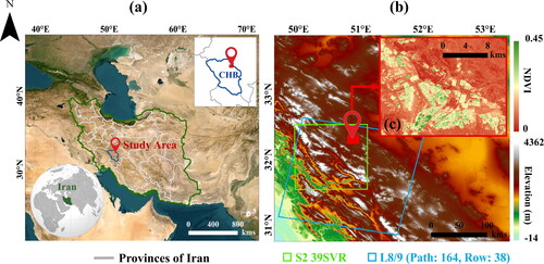
The current paper selected Shahrekord (SHK) city as the study area which is in Chaharmahal and Bakhtiari (CHB) province in the southwest of Iran (Figure 1a). SHK is situated in the eastern part of the Zagros Mountain range, with an average elevation of 2100 m above sea level (Figure 1b). The region experiences hot, arid summers and cold, snowy winters, with an average annual temperature of 11.7 °C and an annual rainfall of 113 mm. The city has a population of approximately 400,000 people (D. Huang et al. 2021). The study site consists of various land cover classes, including agricultural lands, soil and bare lands, urban areas, gardens, and trees (as shown in the 10-year average Normalized Difference Vegetation Index (NDVI) of this region (Figure 1c)). The region plays a significant role in contributing to the overall agricultural yield of the province and southwest parts of Iran. Both mono-cropping and double-cropping cultivation methods are employed for all croplands in this region. This means that both autumn and spring crops are cultivated. The main autumn crops include wheat and barley, while the main spring crops consist of corn, potatoes, and sugar beets. Additionally, alfalfa is another notable agricultural product cultivated in this region. Alfalfa exhibits a distinct pattern compared to other crops as it remains on a farm for multiple years after cultivation. Furthermore, unlike other autumn and spring crops, alfalfa is also harvested multiple times within a CY. Therefore, it is treated as a separate class in this paper, which is fully described in Section 2.3. The planting of autumn crops usually begins in November each year, while the harvesting of spring crops continues until almost the end of October the following year. Therefore, the complete CY in this region spans from November to the end of October of the following year.

Figure 1. (a) Location of the study site in the southwest part of Iran and Chaharmahal and Bakhtiari province, (b) digital elevation model (DEM) of the study site (negative values of elevation indicate regions with elevations lower than mean sea level) and the orbit numbers of Sentinel-2 (S2) and landsat 8/9 (L8/9) images over the study site, and (c) the 10-year (2013-2023) average normalized difference vegetation index (NDVI) of the study site derived from L8/9.

2.2. Remote Sensing datasets

This research utilized two RS datasets: Sentinel-2 (S2) and Landsat-8/9 (L8/9). The S2 mission is part of the European Space Agency’s (ESA) Earth Observation Copernicus program and involves two identical satellites, S2A (launched on June 23, 2015) and S2B (launched on March 7, 2017) (Drusch et al. 2012). Each satellite operates on a 10-day repeat cycle, which is reduced to 5 days when both satellites are used. Both S2A and S2B are equipped with a Multi-Spectral Instrument (MSI), which captures imagery using 13 spectral bands. However, three of these bands are dedicated to atmospheric applications and were not used in this study. The remaining 10 bands, covering the visible, Near Infrared (NIR), and Shortwave Infrared (SWIR) regions from 496 to 2200 nm were used in this research. The study employed atmospherically corrected Level-2A (L2A) S2 images, which are corrected using the Sen2Cor module to provide Surface Reflectance (SR) values (Main-Knorn et al. 2017). The study area is entirely covered by a single S2 image with an orbit number of 39SVR (Figure 1b). It is important to note that S2 L2A data were only available from the end of 2018 over the study site.

The L8/9 data were also utilized as an additional source of RS data. These missions were launched as part of the Earth observation mission by the US Geological Survey (USGS) on February 12, 2013, and February 10, 2022, respectively (Wulder et al. 2019). Both L8 and L9 missions have a spatial resolution of 30 m. This research used SR products from both missions, which have been corrected for atmospheric effects using the Land Surface Reflectance Code (LaSRC). Each mission provides a temporal resolution of 16 days, which is reduced to 8 days when the data are combined. Therefore, due to their similar spatial, spectral, and temporal characteristics, the combination of L8 and L9 datasets was considered as a single dataset referred to as L8/9 (Masek et al. 2020). Given their similar characteristics, this combination poses no challenges for the ML models and can potentially enhance the accuracy of CIP detection by enriching the phenological information associated with each target class (Kabir et al. 2023). Like the S2 dataset, bands ranging from visible to SWIR in L8/9 were also employed. It is important to note that L9 observations were not available before 2022. Thus, only L8 data were used for 2019, 2020, and 2021. The study area is fully covered by a single L8/9 image acquired in row 38 and path 164 orbit (Figure 1b).

2.3. Ground truth dataset

The proposed framework of this study relies on the supervised classification using ML models; therefore, having reliable GT data for model calibration and validation is crucial. To achieve this, extensive field visits were conducted to hundreds of croplands over three successive CYs: 2020, 2021, and 2022. These field visits ensured an adequate distribution of GT samples throughout the study site. Figure 2a,b illustrate the distribution of the collected GT samples, along with some images captured during the field surveys. The field visits took place in April, May, June, July, August, and September of each year, aligning with the peak growth period of autumn and spring crops in the study area. Each farm was visited multiple times per CY to accurately determine its CIP. During these visits, the corner coordinates of the farms were recorded using a Garmin eTrex 30 GPS device with an accuracy of less than 5 m. To mitigate the mixed pixel effect, the corner pixels were recorded with a minimum distance of 30 m from the surrounding land cover classes. It is worth mentioning that in the study region, autumn crops can rely on both rain-fed and irrigation methods, whereas spring crops and alfalfa are exclusively irrigated. Therefore, efforts were made to encompass both irrigated and rainfed autumn crops within the reference dataset.

Figure 2. (a) Distribution of the collected ground truth (GT) samples in three cropping years (CYs) of 2020, 2021, and 2022, (b) some images captured during the extensive field visits in the study site, and (c) the normalized difference vegetation index (NDVI) distribution of various target classes derived from Sentinel-2 (S2) monthly mean composites in 2021 CY using 2021 GT samples. In the figure, ‘C’ stands for land cover class.

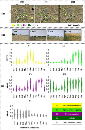
As a result of extensive field surveys, a comprehensive dataset was collected, consisting of five target classes was collected. These target classes are autumn mono-cropping (C1), spring mono-cropping (C2), double-cropping (C3), alfalfa (C4), and other land cover classes (C5). The number of GT samples for each year can be found in Table 1. Alfalfa is a notable agricultural product in the study area, with distinct cultivation and harvesting patterns compared to other crops. Unlike other crops that are harvested once in a CY, alfalfa is harvested multiple times within a CY. Furthermore, if a cropland is cultivated with alfalfa in one CY, it may continue to be under alfalfa cultivation in subsequent CYs. Therefore, a separate class was considered for alfalfa. The other land cover classes (C5) include reference samples of bare soil, urban areas, gardens, and trees. The reference samples for urban areas were mainly derived from high-resolution Google satellite image interpretation. Figure 2c also illustrates the monthly distribution of NDVI values for the various target classes in the 2021 CY (from November to October). These values were derived from monthly mean composites of S2 data using the 2021 GT samples. The graph for C4 demonstrates the distinct pattern of alfalfa compared to other agricultural products. Additionally, autumn crops (in C1 and C3) exhibit their highest level of greenness from April to June, while spring crops (in C2 and C3) reach their greenness peak from July to October.

Table 1. Number of collected ground truth samples in three cropping years: 2020, 2021, and 2022.

Target Classes	Referred to	Number of Reference Samples
		2020	2021	2022
Autumn mono-cropping	C1	768	933	359
Spring mono-cropping	C2	706	1456	288
Double-cropping	C3	111	223	52
Alfalfa	C4	659	713	310
Other landcover classes	C5	1268	1656	576
Total		3512	4981	1585

The dataset for the year 2021 contains a higher number of samples (4981) compared to other years. Consequently, 2021 was selected as the reference year for training the proposed Stack model. During the training phase, 70% of the GT data in each class was utilized for model calibration, while the remaining 30% was set aside for model validation. It is important to emphasize that the validation data did not influence the training process. Subsequently, the trained model was temporally transferred to different years (2019, 2020, 2022, and 2023) to generate CIP maps in those years. To evaluate the model’s temporal transferability, validation was conducted using the entire set of GT samples in 2020 and 2022.

3. Proposed methodology

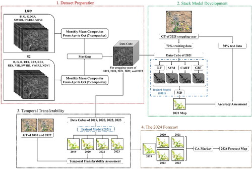
The proposed methodology (Figure 3) includes four main phases: 1) Dataset Preparation, 2) Stack Model Development, 3) Temporal Transferability, and 4) The 2024 Forecast. The following sections provide a detailed description of each phase.

Figure 3. Outline of the proposed methodology. The google earth engine (GEE) JavaScript-based code of the stack model and a part of the ground truth (GT) samples can be found online though the following link https://github.com/ATDehkordi/stack_ensemble_GEE.

3.1. Dataset preparation

This study utilizes the SR values of both S2 and L8/9 RS datasets for CIP mapping. This approach increases the number of observations for each cropland and provides more detailed phenological information for ML models (Shen et al. 2023). S2 L2A data are available from the end of 2018 in GEE (Section 2.2). Hence, this study focuses on mapping different CIPs in the study region from 2019 to 2023. Additionally, L9 observations were not accessible before 2022. Therefore, for the years 2019, 2020, and 2021, only L8 data was utilized. In addition to the spectral bands, this study incorporated NDVI for both S2 and L8/9 datasets. The NDVI is a widely used RS index, especially in vegetation-related studies, as it is highly correlated with the phenological characteristics of crops (Huang et al. 2021). It is calculated using the formula (NIR ̶ R)/(NIR + R) using the NIR and R (Red) bands of satellite images (Bhattacharjee et al. 2021).

Previous studies have shown that using multi-temporal S2 and L8/9 data is more effective than single-date scenarios in providing detailed phenological information and growth patterns (Pluto-Kossakowska 2021). In this study, multi-temporal S2 and L8/9 datasets were used for CIP mapping in each CY. The images were acquired within the complete CY of each year, from November of the previous year to the end of October of the target year. However, since S2 and L8/9 belong to the category of optical RS data, cloud coverage can be a limiting factor (Aljenaid et al. 2022; Singh et al. 2022). Thus, only satellite images with less than 10% cloud coverage were considered from the entire collection of S2 and L8/9 data over the study site. Potential cloudy pixels were also identified and removed from each image using the pixel quality attributes provided with S2 ('QA60' band) and L8/9 ('QA_PIXEL' band) data (Kumar and Mehta 2023). In some months of the target CYs (2019-2023), no images could be found with less than 10% cloud coverage. Moreover, the process of cloud removal may result in data gaps within the RS datasets.

Since the study aims to utilize the temporal transferability of the proposed Stack model to generate CIP maps in different years (from 2019 to 2023), it is crucial to ensure that the input features of the ML models remain consistent and similar across all years. To achieve this, the study employed the monthly mean composites of S2 and L8/9 data from April to October, resulting in a total of 7 composites for each dataset. This period was chosen as it provided gap-free datasets over the study area for all target CYs and coincides with the peak of greenness for both autumn and spring products, thereby incorporating critical phenological information into the input features of the ML models. The process of mean compositing also helps to mitigate potential data acquisition- and sensor-related noise present in the images (Selvaraj and Pérez 2023). The monthly composites of S2 data were resampled using the bilinear technique to match the spatial resolution of L8/9 data (Silvero et al. 2021; Wang et al. 2022). Subsequently, the data from both sources were stacked together, resulting in a 30-meter data cube for four consecutive CYs (from 2019 to 2023). Each data cube was utilized separately to generate the CIP map of the study site in the target years. The proposed Stack ensemble model is introduced in the next phase, which employs the 2021 data cube and GT samples for model calibration.

3.2. Stack model development

This study proposes a Stack ensemble of ML models for classifying CIPs in GEE. The proposed Stack model combines the predictions of multiple base classifiers using a meta classifier to generate the final prediction. To ensure diversity in the Stack model, RF, SVM, GBT, and CART were selected as the base classifiers, as each model has its unique characteristics. Additionally, the MD classifier was also selected as the meta model because simple linear models can achieve higher accuracies in the Stack architecture (Alazba and Aljamaan 2021). It is important to note that although GEE has facilitated the process of RS datasets by providing an online cloud-based platform, these five ML models were the main classifiers provided by GEE at the time of conducting this research. In the proposed Stack approach, all base classifiers were trained separately using the same training data. The outputs of the base classifiers are probabilities that indicate the likelihood of a sample belonging to different target classes (C1-C5). The meta classifier, trained using the same training dataset as the base models, utilizes these probabilities to determine the final class of a sample.

The RF utilizes an ensemble of decision trees to make predictions (Breiman 2001). Each decision tree within the RF is trained on a different subset of the training data and generates its prediction. Once all the decision trees have been trained, the RF combines their individual predictions through a voting mechanism. In classification tasks, the class with the highest number of votes is chosen as the final prediction. RF involves several main input hyperparameters that need to be determined (Table 2).

Table 2. The Input hyperparameters of different classifiers used in the proposed Stack model.

Model	Hyperparameter	Description	Grid search space
RF	Number Of Trees	The number of decision trees to create.	[10, 50, 100, 200, 300]
	Variables Per Split	The number of variables per split.	[1-5, step = 1]
	Max Nodes	The number of leaf nodes in each tree.	[1-5, step = 1]
SVM	G	The gamma value in the kernel function.	[1, 5, 10, 100, 1000] × ${10}^{-4}$
	C	The cost parameter	[1, 10, 100, 1000, 10000] × ${10}^{-3}$
GBT	Number Of Trees	The number of decision trees to create.	[10, 50, 100, 200, 300]
	Shrinkage	This parameter controls the learning rate.	[1, 10, 100, 1000] × ${10}^{-4}$
	Max Nodes	The number of leaf nodes in each tree.	[1-5, step = 1]
CART	Max Nodes	The number of leaf nodes in each tree.	[1-5, step = 1]
	Min Leaf Population	Nodes with at least this many points.	[1-20, step = 2]
MD	Distance Metric	The distance metric to use.	'Euclidean’, 'Cosine’, 'Mahalanobis’, 'Manhattan’

The SVM aims to identify an optimal hyperplane that effectively separates different classes within the input feature space (Hearst et al. 1998). By finding the best hyperplane, SVM can efficiently handle data that is not linearly separable. This is achieved by the kernel trick, where a kernel function projects the input feature space into a higher-dimensional space. In this higher-dimensional space, the classes can be separated by a hyperplane. One of the most used SVM kernels is the Radial Basis Function (RBF), employed in this study. The other main input parameters of SVM are presented in Table 2.

The GBT is an ensemble learning technique that sequentially combines multiple decision trees to make predictions (Friedman 2001). It is built on the concept of boosting, which involves training multiple weak learners, typically decision trees with shallow depths, to enhance the overall predictive accuracy. The GBT utilizes gradient descent optimization during the iterative training process of each weak learner. The main input hyperparameters of GBT are also summarized in Table 2.

The CART constructs a decision tree model for making predictions based on input features (Breiman et al. 1984). It utilizes a splitting criterion, which assesses the distribution of classes within a node, to determine the optimal division of data at each internal node. The CART follows a recursive partitioning technique to build the decision tree, iteratively splitting the data based on the selected splitting criterion. It creates a hierarchical structure of decision nodes and leaf nodes, where each decision node represents a feature and a corresponding splitting condition, and each leaf node represents a predicted class or value. The input hyperparameters of this model in GEE are also displayed in Table 2. The MD classifier falls under the category of distance-based classifiers (Hodgson 1988). In the classification phase, the MD classifier calculates the distance between the feature vector of an unlabeled data point and the GT samples of each class. It then assigns the unlabeled data point to the class whose sample is closest in terms of distance. The distance metric in this approach can also be determined (Table 2).

The dataset for the year 2021 had a larger number of samples (4981) compared to other years (Table 1). Therefore, 2021 was selected as the reference year for training the Stack model. During the training phase, 70% of the GT data from each class in 2021 were randomly chosen for model calibration, while the remaining 30% was held out for model validation. It is important to note that the validation data did not influence the training process. To determine the optimal hyperparameters for each ML model (Table 2), a grid search approach was employed using 5-fold cross-validation on the training data (70% of GT samples in 202). Once the optimal hyperparameters were identified, each model was trained using the entire set of training data. For model development in 2021, the corresponding data cube of 2021 was used as the input for the Stack model. In the next phase, the trained model from 2021 is utilized to generate CIP maps for the years 2019, 2020, 2022, and 2023, using the corresponding prepared data cubes (Section 3.1).

3.3. Temporal transferability

This study uses a trained Stack model from 2021 to create CIP maps for the years 2019, 2020, 2022, and 2023 from the corresponding data cubes of these years (Section 3.1). It is important to highlight that, the proposed methodology employed mean monthly composites of S2 and L8/9 data to generate RS data cubes. This approach was chosen not only for the reasons outlined in Section 3.1 but also because mean compositing provides a better assurance of feature similarity and consistency across different years, boosting the performance of CIP mapping in different years using the proposed Stack model. By leveraging patterns and relationships learned from the 2021 training data, the model accurately predicts data for multiple years without any excessive GT samples. This approach saves time and resources, while still providing valuable predictions for different periods. To evaluate the temporal transferability of the proposed Stack model, all the GT data from 2020 and 2022 were used for validation. None of the data from 2020 and 2022 interfered with the training of the Stack model. Having CIP maps from multiple years is also crucial for forecasting future CIP maps, as the time series of maps captures change patterns that can be used to model the CIP map for the following year. Next, the generated time series of CIP maps from 2019 to 2023 is used to model the CIP map of 2024.

3.4. The 2024 forecast

It is possible to generate a forecast map for 2024 using the time series of generated CIP maps from 2019 to 2023, with the help of the CA-M chain model. It is worth noting that the CA-M model has not yet been utilized for forecasting future CIP maps. However, it is widely employed for modeling both spatial and temporal changes in land cover types, aiming to foster sustainable land use development (Jana et al. 2022; Arfasa et al. 2023).

The CA-M approach combines the CA and Markov chain models. The CA model captures the spatial dynamics of changes in the target classes by using the concept of cells (Norris 2012). The model takes into account the current state of a cell and its neighboring cells to determine the transition rules for updating the state of that cell in the subsequent time step. These transition rules are established based on the spatial patterns and rules observed in previous CIP maps within the study area. On the other hand, the Markov chain model characterizes the temporal dynamics of changes in the target classes (Norris 2012). The construction of the Markov chain is based on the observed historical transitions from one target class to another. The transition probabilities within the chain indicate the likelihood of a target class transitioning to another class in the next time step. The CA-M model takes into consideration both the local interactions among neighboring cells and the overall temporal trends observed in the transitions of the target classes. In this study, the number of iterations for the CA model was set to 10, as this has yielded the best results in forecasting future land use/cover maps (Jana et al. 2022). Additionally, the standard 5 × 5 mean contiguity was employed for the CA-M model (Jana et al. 2022). To evaluate the accuracy of the CA-M model in CIP mapping in 2024, a map was first generated for 2023 using the previous Stack-derived CIP maps from 2019 to 2022 (referred to as 2023_CA-M). This map is then compared to the reference map of 2023 derived from the proposed Stack model (referred to as 2023_Stack). This comparison serves to demonstrate the effectiveness of the CA-M model in modeling CIP changes. Once the performance of the CA-M model has been validated, it is utilized to forecast the 2024 CIP map.

3.5. Evaluation metrics

To quantitatively assess the performance of the Stack model in 2021 and evaluate its temporal transferability in 2020 and 2022, the classification results were analyzed using the Confusion Matrix (CM) of the validation data and various CM-derived metrics. These metrics include Overall Accuracy (OA), Kappa coefficient, Producer’s Accuracy (PA), User’s Accuracy (UA) and F1-score.

The performance of the CA-M model in generating the 2023 CIP map (referred to as 2023_CA-M) was evaluated by comparing it with the CIP map generated by the proposed Stack model for 2023 (referred to as 2023_Stack). The evaluation involved the use of several Kappa metrics and Quality Disagreement (QD) and Allocation Disagreement (AD) parameters (Table 3). It is recommended that Kappa metrics alone might not be sufficient for suitable validation of the CA-M model in forecasting CIP maps. Therefore, QD and AD were also calculated by comparing the entire 2023_CA-M map with the 2023_Stack map. The Kappa metrics (K_no, K_std, and K_loc) have a range of 0 to 1, where a value of 1 indicates perfect agreement between the forecast map and the reference map, and a value of 0 indicates no agreement better than chance. For QD and AD, lower values closer to zero indicate a better match between the forecasted and reference CIP maps. Additionally, the coefficient of determination (R²) was used to compare the total area of each class between the 2023_CA-M and 2023_Stack maps.

Table 3. Metrics for performance evaluation of CA-M model in forecasting CIP maps.

Metric	Description
Kno	This refers to the Kappa coefficient for no information, which assesses the overall agreement between the forecasted map and the reference map.
Kstd	This is the conventional Kappa Index of Agreement, which compares the observed proportion of correct classifications to the expected proportion of correct classifications without the ability to accurately specify the location.
Kloc	This is the Kappa coefficient for pixel-level location, which measures the success rate of accurately specifying the location. It is used to compute the spatial accuracy in the overall landscape.
QD	This parameter assesses how similar a forecasted map is to a reference map in terms of the quantities (number of pixels) of different classes.
AD	This assesses how similar a forecasted map is to a reference map in terms of the spatial allocation of different classes.

For more information, please see (Pontius 2000) and (Pontius & Millones 2011).

4. Results

4.1. Performance of stack model

The hyperparameters of various algorithms within the Stack model were initially tuned using 5-fold cross-validation on the training data from 2021 (Section 3.2). Subsequently, the entire training dataset was utilized to train the Stack model in 2021. It is important to note that, for the 2021 dataset, a combination of S2 and L8 datasets was utilized, as L9 data was not available in 2021.

Figure 4 depicts that the proposed Stack ensemble model performs better than other ML models in terms of OA and Kappa. The Stack model achieved an OA of 94.24% and a Kappa of 0.92, which is approximately 3.7% and 0.05 better than the second-best performing model, RF, which had an OA of 90.56% and a Kappa of 0.87. The poorest performing model was MD, with an OA of 78.59% and a Kappa of 0.71. SVM, GBT, and CART ranked third to fifth in terms of OA and Kappa for CIP classification. The results suggest that the proposed Stack model is the best choice for CIP classification among all the other ML models considered in this study.

Figure 4. Performance evaluation of different machine learning models using validation data in 2021 (30% of the ground truth samples in 2021).

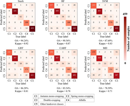
The findings also suggest that the proposed Stack model reduced both omission and commission errors in the identification of target classes (Figure 4). The values of UA, PA, and F1-scores derived from the CMs in Figure 4 are also illustrated in Figure A1 for better interpretation. For example, for C1 with 280 validation samples, the Stack model accurately classified 264 of them, while the other classifiers achieved values of 257, 243, 241, 236, and 219, respectively. This indicates that the Stack model outperformed the others in accurately classifying C1. The superior performance of the proposed Stack model is further evidenced by the F1-scores displayed in Figure A1. For instance, the F1-scores for classes C1 to C5 are 93.28% for C1, 98.27% for C2, 88.57% for C3, 92.73% for C4, and 92.72% for C5. These scores surpass those of the RF model, the second-best performing model, which achieved F1-scores of 90.65% for C1, 95.77% for C2, 73.38% for C3, 88.76% for C4, and 89.67% for C5. Consequently, it can be concluded that the Stack model enhances the performance of all base models across all target classes, with class C3 showing the most significant improvement of approximately 15%. These results the Stack model’s ability to improve the UA and PA of different target classes, resulting in the highest OA and Kappa compared to other ML models.

To demonstrate the effectiveness of the proposed Stack structure, which comprises CART, GBT, SVM, and RF as base classifiers, various scenarios were tested (Figure 5). In these experiments, the meta classifier was fixed as MD, as it is recommended for the meta classifier to be a simple classifier (Section 3.2). It is evident that the Stack ensemble structure improved the final OA compared to the single-classifier scenarios, regardless of the number of base classifiers. For instance, the best single classifier, RF, achieved an OA of 90.56%. However, when combined with CART (CART + RF), GBT (GBT + RF), and SVM (CART + RF) in the two-base classifier scenarios, the OA increased to at least 91.59%. This trend is also observed in the three-base classifier scenarios. For example, CART + GBT + RF achieved an OA of 92.58%, which is higher than the individual OAs of these base classifiers. The proposed Stack model with the four base classifiers yielded the best performance, achieving an OA of 94.24%. Therefore, the structure of CART + GBT + SVM + RF as the base classifiers and MD as the meta learner was selected as the proposed structure in this paper.

Figure 5. Analysis of the structure of the proposed stack model compared to different scenarios.

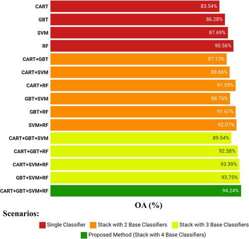
RF can also be considered as the primary contributor to the improvement of classification OA in the proposed Stack structure. This is evident when comparing the scenario of CART + GBT + SVM, where the OA is 89.54%. By including RF as one of the base classifiers, the OA increases by 4.7% (resulting in an OA of 94.24% for CART + GBT + SVM + RF). SVM ranks second in terms of contribution, as the OA of CART + GBT + RF increases by 1.66% compared to the scenario with all four base classifiers. GBT follows as the third, contributing an increase of 0.85% to the OA of CART + SVM + RF in the four-base classifier scenario. CART, on the other hand, only has a marginal impact, increasing the OA by 0.49% from 93.75% (GBT + SVM + RF) to 94.24% (four-base classifier scenario). The greater impact of RF can also be observed in the three-base classifier and two-base classifier scenarios. This prominence of RF compared to other classifiers can be attributed to its higher OA, while the other classifiers contribute in the same order as their individual OAs in single scenarios.

In the proposed Stack structure, both S2 and L8 RS datasets were used for 2021 (L9 data were not available during this period). Figure 6 shows that when both S2 and L8 were used, the Stack model achieved an OA of 94.24% and a Kappa of 0.92. However, when only S2 was utilized, both OA and Kappa decreased to 91.37% and 0.88, respectively. On the other hand, employing only L8 resulted in the poorest performance for the proposed Stack model, with an OA of 88.56% and a Kappa of 0.84. These findings highlight that the multi-sensor classification of CIPs yields higher accuracies compared to single-source approaches. Additionally, S2 demonstrates superior performance over L8 in identifying the target classes.

Figure 6. Effect of using Sentinel-2 (S2) and Landsat-8 (L8) remote sensing datasets in the proposed Stack model using validation dataset in 2021.

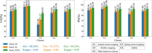
The utilization of both S2 and L8 datasets resulted in the highest PAs and UAs across all target classes. In terms of PAs, class C4 showed the greatest improvement when both S2 and L8 were employed, with enhancements of 4.67% and 10.28% compared to the S2-only and L8-only cases, respectively. For UAs, the most significant increase was observed in class C3, where UA improved from 63.04% (L8-only) and 73.17% (S2-only) to 84.93% when both S2 and L8 were utilized. These findings demonstrate the superior performance of the multi-source input features in the Stack model compared to using a single source.

4.2. Temporal transferability

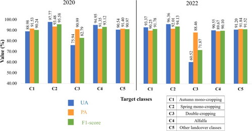
The Stack model trained in 2021 was temporally transferred to the years 2019, 2020, 2022, and 2023 to generate CIP maps using the corresponding prepared data cubes (Section 3.3). Table 4 indicates that when temporal transferability is employed, the proposed Stack model achieves the highest classification accuracies. In 2020, it obtained an OA of 91.82% with a Kappa value of 0.89, while in 2022, it achieved an OA of 90.97% with a Kappa value of 0.87. Compared to the second-best model, RF, the Stack model outperforms by approximately 4.5% and 5.3% in terms of OA in 2020 and 2022, respectively, demonstrating its superior performance in temporal transferability. These results indicate that the proposed Stack model exhibits better generalization to different years and provides more reliable outcomes compared to other ML models. CMs of 2020 and 2022 in Figure 7 also depict that the majority of samples are correctly classified, confirming the feasibility of temporal transfer of the proposed Stack model to generate time series maps of CIP for different years. The values of UA, PA, and F1-scores derived from the CMs in Figure 7 are also illustrated in Figure A2 for better interpretation. Among the target classes, C2 achieved the highest F1-scores in both 2020 and 2022, with values of 95.58% and 94.13%, respectively. Conversely, C3 recorded the lowest F1-scores, with values of 82.79% and 71.87%. These results are consistent with those from 2021 (Figures 4, 6, and Figure A2), where C2 was the most accurately detected class and C3 was the least accurate among the target classes.

Figure 7. Confusion matrices of validating the proposed Stack model using the complete ground truth samples in 2020 and 2022.

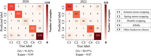
Table 4. Temporal transferability of different MLs using the complete GT samples of 2020 and 2022 (Table 1).

Year	Metric	Stack	RF	SVM	GBT	CART	MD
2020	OA (%)	91.82	87.32	85.94	85.82	80.35	74.47
	Kappa	0.89	0.85	0.82	0.79	0.76	0.69
2022	OA (%)	90.97	85.68	84.91	84.55	78.95	71.22
	Kappa	0.87	0.83	0.82	0.78	0.74	0.65

The effectiveness of temporal transfer depends on the similarity and consistency of input data cubes of RS images across different years (Section 3.3). To achieve this, monthly mean composites of S2 and L8/9 datasets were utilized in this study, ensuring an equal number of features for the classification of CIPs. The high values of OAs and Kappas in 2020 and 2022 (Figure 7) also demonstrate the success of mean compositing in consistently representing the dynamics of CIPs monthly. In other words, this approach enables the generation of consistent features across target years, ensuring accurate mapping of CIPs.

Figure 8 also shows that the proposed Stack model successfully generated CIP maps through temporal transfer. The maps exhibit low point-based noise, which is common in pixel-based classification techniques. It is evident that the majority of the cultivated area each year falls into the C1 category, as autumn crops like wheat and barley play a crucial role in ensuring food security. Following C1, C2 emerges as the most common CIP across all years in the study area. C3 and C4 alternate in the third and fourth places in different years. Among the target years, 2020 recorded the highest total cultivated area, reaching 7123.22 ha. The significant increase in the area of C1 class, which includes both irrigated and rainfed crops like wheat and barley, in the study region over the past five years can be attributed to the unusually high levels of precipitation experienced at the end of 2019 (Sherpa and Shirzaei 2022). On the other hand, 2022 exhibited the lowest cultivation area, with an area of about 6177.97 ha. There is an overall declining trend in total cultivation areas which can be attributed to the water scarcity problems of the region (Taheri Dehkordi et al. 2022, 2022).

Figure 8. Cropping Intensity Pattern (CIP) maps of 2019-2023 derived from the proposed methodology. All the area units are in hectares (ha).

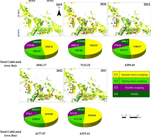
It can be concluded that the area occupied by CIPs consisting of irrigated-only crops, specifically C2 (where all spring products are irrigated), C3 (where all spring products are irrigated), and C4 (where alfalfa is irrigated), has shown a consistent downward trend (Figure 8). This trend is particularly noticeable in C2 and C3, where the areas have decreased from 1501.07 ha to 1171.94 ha and from 1129.84 ha to 917.53 ha, respectively. The decline in these CIPs can be attributed to the significant reduction in water resources in the region, as reported in previous studies (Taheri Dehkordi et al. 2022). The area occupied by C4, which involves the cultivation of alfalfa, has exhibited more stability over time. This is because when a farm is cultivated with alfalfa, it can be harvested for multiple years. On the other hand, the C1 category, which includes both irrigated and rainfed crops, displays the highest variability across the years due to the dependence of rainfed crops on seasonal precipitation patterns.

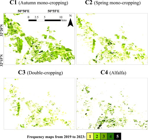
Frequency maps of Figure 9 indicate that a considerable portion of the croplands in the study site was classified as C1 (autumn mono-cropping) due to the cultivation of crops like wheat and barley, which fall under the C1 CIP. The second most frequently occurring CIP in the study site was C2, while C3 and C4 were less common. Notably, the frequency of croplands classified as C4 was higher than other CIPs. This can be attributed to the fact that when a cropland is cultivated with alfalfa, it often remains dedicated to alfalfa cultivation for several consecutive years.

Figure 9. Frequency maps of target classes from 2019 to 2023 derived from the proposed methodology. Each map displays the number of times that various locations within the study area being classified as the target classes over a span of five years (2019-2023).

4.3. The 2024 forecast

The proposed Stack ensemble model was used to generate a time series of CIP maps for the study site from 2019 to 2023. Subsequently, the CA-M model was employed using the previous maps to forecast the CIP maps for 2023 and 2024. To evaluate the performance of the CA-M model in forecasting the 2024 map, the CIP map of 2023 generated by the CA-M model (2023_CA-M) was compared with the CIP map derived from the Stack model (2023_Stack). Based on visual inspection (Figure 10), it is evident that CA-M successfully and accurately forecasted the CIP map of 2023 based on the previous CIP maps. Additionally, Table 5 provides the values of evaluation metrics used to compare 2023_CA-M and 2023_Stack. The Kappa metrics attained values exceeding 0.78, while QD (0.01) and AD (0.06) exhibited low values close to zero. The values of these metrics collectively indicate minimal differences and a high level of consistency between the two CIP maps.

Figure 10. Comparison of 2023 Cropping Intensity pattern (CIP) maps derived from the proposed stack (2023_Stack) model and cellular Automata-Markov (CA-M) (2023_CA-M) model. The forecasted CIP map of 2024 using CA-M model is also provided (2024_CA-M).

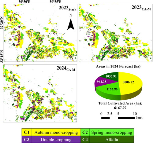
Table 5. Evaluation metrics, used to compare 2023_CA-M and 2023_Stack.

Evaluation Metrics
Kno	Kloc	Kstd	QD	AD
0.91	0.80	0.78	0.01	0.06

The effectiveness of the CA-M model is further demonstrated by comparing the cultivation areas of different target classes in the 2023_CA-M and 2023_Stack (Table 6). The results revealed a strong correlation (R² = 0.98) between the areas obtained from the two maps. Additionally, the relative forecast error between the two maps using the CA-M model was less than 20% in all classes, compared to the 2023_Stack. These findings prove the accurate performance of the CA-M model in forecasting CIP maps. Consequently, it is expected that the 2024 map is also relatively accurate.

Table 6. Comparison of the areas of target classes derived from 2023_CA-M and 2023_Stack.

Year	Model	Area (ha)				R^2
		C1	C2	C3	C4
2023	Stack	3745.84	1371.94	917.53	1183.83	0.98
	CA-M	3016.04	1516.34	879.43	1192.55
Relative Error (%) [(AreaCA-M – AreaStack)/AreaStack]		−19.48	10.52	−4.15	0.73

According to the forecasted CIP map of 2024 (2024_CA-M in Figure 10), a total cultivation area of approximately 6200 ha is anticipated for 2024, with C1 remaining the dominant CIP in the study region, covering an area of approximately 3000 ha. While there may be some errors in the 2024 forecasted map, as other parameters such as precipitation, temperature, and soil conditions must be considered for accurate future CIP mapping, it still offers valuable insights into the study site. These insights can aid in informed decision-making, water management, and ensuring food security within society.

5. Discussion

5.1. Multi-source CIP mapping

This article proposed a methodology that combines S2 and L8 data for improved accuracy in CIP mapping. The results demonstrate that using a multi-source approach leads to better results (Figure 6). This is because S2 and L8 data are collected on different dates, allowing each sensor to complement the other and capture the phenological dynamics of various CIPs more comprehensively. Similar results have been reported in other agricultural studies, highlighting the superior performance of combining S2 and L8 (Shen et al. 2023). However, this combination has not been widely used in CIP mapping. Most papers only focus on crop type classification. Other studies reported improved CIP classification by incorporating other sources of RS data. For instance, in one study, a combination of Gaofen-1 and MODIS satellite data led to increased classification accuracy (Xiang et al. 2019). It is worth noting that S2 data achieved higher accuracies compared to L8/9 when used for CIP mapping alone. This is due to the richer spectral information and denser temporal resolution (5-day interval) offered by S2 in comparison to L8 data (Wang et al. 2022).

5.2. Proposed stack ensemble model

This study introduced a novel ensemble framework for ML models known as the Stack model. The Stack model performs better than any of its constituent ML models (Figure 4 and Figure A1). However, some studies were unable to create ensemble models capable of surpassing the performance of each individual base ML model, which depicts the superiority of the proposed Stack model (Vasilakos et al. 2020). In other studies, plenty of ML models were used in the ensemble structure to improve the classification accuracy (Rahmati et al. 2022). In contrast, the proposed Stack model leverages only five ML models to enhance the accuracy of CIP classification. Notably, the superior performance of the Stack model extends beyond 2021 and exhibits consistent excellence when is temporally transferred to different years (Table 4, and Figure 7 and Figure A2). The proposed Stack model demonstrates superior performance due to several contributing factors: 1) The Stack model is a type of heterogeneous ensemble model that combines predictions from various base classifiers using a meta classifier. This diversity enables the model to capture a broad range of complex patterns and relationships in the data, leading to improved performance. 2) Stacking allows for adjusting predictions from the base models. The stack ensemble can learn to correct errors or biases present in individual base models, while the meta classifier can identify and weigh the predictions based on their reliability, mitigating the impact of individual model weaknesses. 3) Thirdly, the Stack ensemble demonstrates excellent generalization to unseen data by leveraging collective knowledge from diverse base models, which explains its superior performance in temporal transferability.

The results presented in Figure 4 and Figure A1, and Table 4 clearly indicate that the RF model outperformed other models such as GBT, SVM, CART, and MD in the mapping of CIPs. While there have been few studies utilizing ML models for CIP mapping, RF has consistently demonstrated superior performance compared to other ML models in landcover classification and crop type mapping (Palanisamy et al. 2023; Tariq et al. 2023). The superior performance of RF in this study can be attributed to several factors. Firstly, the ensemble nature of RF, which combines multiple decision trees, helps to mitigate the biases and variances associated with individual trees (Saini and Ghosh 2017). Secondly, RF has the ability to capture complex, non-linear relationships in the data by randomly selecting subsets of features and training decision trees on these subsets (Maxwell et al. 2018). This flexibility allows RF to effectively model the intricate patterns present in the CIP data. Lastly, the random feature selection and bootstrapping techniques employed in RF contribute to robustness by reducing the impact of noisy or outlier observations and minimizing the risk of overfitting to the training data (Zhang et al. 2022).

The proposed Stack model in this study has achieved remarkable accuracies in classifying CIPs. The model outperformed the state-of-the-art results reported in previous articles. For instance, previous studies using MODIS and Gaofen-1 data reported OAs of approximately 62% and 78%, respectively (Xiang et al. 2019). Another study reported an average OA of 89% for mapping different classes of CIPs (Liu et al. 2021). A recent article utilizing GEE and analyzing the peaks of temporal MODIS NDVI profiles achieved an OA of 85.3% (Gumma et al. 2022). In contrast, the proposed method in this research yielded an OA of around 95% during the training year. Even when transferred to other years without extensive training data, it still achieved a high OA of approximately 91%.

5.3. Temporal transfer

The superior performance of the Stack model allowed for the generation of CIP maps for different years without the need for extensive GT data collection, which is both costly and time-consuming. Moreover, even with sufficient resources for GT data collection, producing CIP maps for past years would be unfeasible. However, temporal transferability allows for the effective mapping of CIPs in previous years. By utilizing a time series of CIP maps, forecasting models, such as CA-M, can be employed to generate a 2024 map. The success of CA-M in forecasting CIP maps (Tables 5 and 6) can be attributed to the temporal transferability of the Stack model, which could generate highly accurate CIP maps for different years. Although the 2024 forecast map may contain certain inaccuracies, as it does not account for other influential factors such as precipitation, temperature, and soil conditions necessary for precise future CIP mapping, it still provides significant and valuable insights into the study site. These insights can be instrumental in making informed decisions, managing water resources effectively, and ensuring food security for society.

The Stack model’s remarkable accuracies also validate the suitability of using monthly mean composites of S2 and L8/9 data to maintain consistency in input features across different years (Figure 7 and Figure A2). Essentially, this approach ensures a more uniform and stable representation of the target classes, thereby enhancing the model’s capacity to generalize across various years. By averaging pixel values over a month, mean monthly compositing produces a smoother and less noisy depiction of the target classes, resulting in a more accurate representation. Additionally, mean compositing aids in reducing the impact of cloud cover and atmospheric conditions, further enhancing the model’s performance.

5.4. Confusion between target classes

In general, the Stack model proved to be effective in classifying the target classes (Figure 6). However, there are still cases where confusion arises between the target classes (Table 7). It is important to mention that there could be additional confusion in CIP classification that has not been summarized. Nonetheless, Table 7 provides a comprehensive overview of the challenges faced in CIP classification, offering valuable insights into the topic.

Table 7. Possible confusions between the target classes of this study.

Target class	Discriminative characteristic	Main possible confusion with	Reason
C1	Low greenness at the end of CY	C5 (grasslands and pastures)	- Similar greenness values in spring.
C2	Low greenness at the beginning of CY	C3	- Exhibition of greenness by C2 in the spring caused by the growth of crop residue from previous CY
C3	Low greenness between the autumn product harvest and spring product cultivation	C2, C4, and C5 (trees and gardens)	- Smaller number of training samples - Monthly mean features may not fully capture discriminative characteristic*
C4	High greenness throughout the CY	C3 and C5 (gardens and trees)	- High greenness throughout the CY by C3 and C5 (gardens and trees)
C5	Mainly low NDVI values (except vegetation-related subclasses)	C1	- High intra-class variability of C5.

* Explanation: The reason why the utilization of both Sentinel-2 and Landsat 8/9 data led to the highest increase in User’s Accuracy (UA) for C3 (Figure 6) because of enriching phenological information.

5.5. Future perspectives

The entire study was designed and implemented using the functionalities provided by GEE, which offers a wide range of RS datasets, significant computational resources, and multiple algorithms (Gorelick et al. 2017; Taheri Dehkordi et al. 2022). One of the key advantages of GEE is its ability to process satellite data online, eliminating the need for manual downloads. Since the datasets and methods employed in this research are publicly available within the GEE platform, the proposed approach can be implemented in large-scale and long-term studies thanks to the high-performance computing and parallel processing capabilities offered by GEE (Huang et al. 2017). For future studies, an ensemble deep learning model will be developed to further improve the mapping of CIPs. However, it is important to note that users will need to process the data locally or utilize the capabilities of Google Colab, as GEE did not support deep learning models at the time of conducting this research. The scope of this paper was limited to assessing the temporal transferability of the proposed model within a specific region, stemming from the lack of reference samples in other regions. Future research can focus on evaluating deep learning-based ensemble models in both temporal and spatial contexts. By expanding the evaluation to encompass both dimensions, a more comprehensive understanding of the model’s performance can be obtained. Moreover, implementing data augmentation techniques to increase the number of training samples for different classes can also be pursued (Hao et al. 2023). Additionally, the inclusion of additional data sources such as Sentinel-1 (S1) can be beneficial. S1 data provides valuable information regarding the structure, geometry, and moisture content of various crops, which can significantly improve the classification accuracy of CIP detection (Sherpa and Shirzaei 2022). This paper only evaluated the temporal transferability of the proposed model in the same region. Future research can focus on evaluation deep learning-based models both temporally and spatially.

6. Conclusions

Monitoring the dynamics of CIPs is crucial due to rapid population growth, climate change, and increased demands. In this study, S2 and L8/9 data from 2019 to 2023 were utilized to generate CIP maps for the southwestern regions of Iran. To accurately detect CIPs, a Stack ensemble structure of ML models was developed, considering the high inter- and intra-class variabilities of CIPs. The Stack model employed RF, SVM, GBT, and CART as base classifiers, with MD as the meta model. The Stack model was trained in 2021 using GT samples from the same year, and the validation results in 2021 indicated its superior performance compared to each individual ML base model. The findings also suggested that utilizing multi-source classification (combining S2 and L8/9 data) yielded more accurate results than single-source classification (S2-only or L8-only). The trained Stack model from 2021 was then used to generate CIP maps for the years 2019, 2020, 2022, and 2023. The temporal transferability of the model was evaluated using the GT dataset from 2020 and 2022, confirming its effectiveness in generating accurate CIP maps without excessive GT data. By generating an accurate time series of CIP maps from 2019 to 2023, the CA-M model was employed to forecast the 2024 map, which provides valuable insights in land use planning and decision-making processes. The CA-M model’s performance was validated by comparing its 2023 map with the 2023 map derived from the Stack model. The results exhibited a strong agreement between the CA-M and Stack maps in 2023, indicating the efficacy of the CA-M model. This study provides valuable insights into the monitoring and forecasting of CIPs, which play a critical role in ensuring food security, shaping water management policies, and fostering environmental conservation. The proposed methodology can be applied by researchers and scientists worldwide to investigate long-term changes in CIPs across various regions.

Authors’ contributions

Marziyeh Majnoun Hosseini and Alireza Taheri Dehkordi: Conceptualization, Methodology, Software, Data collection, Data processing and analysis, Visualization, Writing – original draft. Mohammad Javad Valadan Zoej and Ebrahim Ghaderpour: Supervision, Writing – review & editing.

Acknowledgments

The authors would like to express their genuine gratitude to ESA, NASA, and USGS for their support of the Sentinel and Landsat programs, which offer valuable earth-observed data to researchers and scientists globally. The authors also extend their appreciation to the GEE team for providing an online cloud processing platform that contains vast amounts of remote sensing data. The authors acknowledge the Department of Earth Sciences at Sapienza University of Rome for their support through “Progetto dipartimentale”.

Disclosure statement

No potential conflict of interest was reported by the authors.

Data availability statement

The complete dataset associated with this study can be accessed by submitting a request to the corresponding author. The GEE source code of the Stack model and a part of the GT samples can be found at https://github.com/ATDehkordi/Stack_ensemble_GEE.

Additional information

Funding

This research has received no external fundings.

APPENDIX

Figure A1. User’s accuracy (UA), producer’s accuracy (PA), and F1-score values for performance evaluation of different machine learning models using validation data in 2021 (30% of the ground truth samples in 2021).

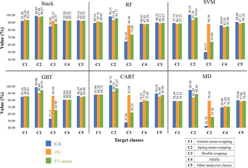
Figure A2. User’s accuracy (UA), producer’s accuracy (PA), and F1-score values for validating the temporal transfer of the model trained in 2021 to the years 2020 and 2022, using the complete ground truth samples from both years.

References

- Abdali E, Valadan Zoej MJ, Taheri Dehkordi A, Ghaderpour E. 2023. A parallel-cascaded ensemble of machine learning models for crop type classification in google earth engine using multi-temporal sentinel-1/2 and landsat-8/9 remote sensing data. Remote Sens. 16(1):127. doi: 10.3390/rs16010127.
- Alazba A, Aljamaan H. 2021. Code smell detection using feature selection and stacking ensemble: an empirical investigation. Inf Softw Technol. 138:106648. doi: 10.1016/j.infsof.2021.106648.
- Aljenaid SS, Kadhem GR, AlKhuzaei MF, Alam JB. 2022. Detecting and assessing the spatio-temporal land use land cover changes of Bahrain Island during 1986–2020 using remote sensing and GIS. Earth Syst Environ. 6(4):787–802. doi: 10.1007/s41748-022-00315-z.
- Arfasa GF, Owusu-Sekyere E, Doke DA. 2023. Past and future land use/land cover, and climate change impacts on environmental sustainability in Vea Catchment, Ghana. Geocarto Int. 38(1):1–44. doi: 10.1080/10106049.2023.2289458.
- Bhattacharjee S, Islam MT, Kabir ME, Kabir MM. 2021. Land-use and land-cover change detection in a north-eastern wetland ecosystem of Bangladesh using remote sensing and GIS techniques. Earth Syst Environ. 5(2):319–340. doi: 10.1007/s41748-021-00228-3.
- Breiman L. 2001. Random forests. Machine Learning. 45(1):5–32. doi: 10.1023/A:1010933404324.
- Breiman L, Friedman J, Olshen RA, Stone CJ. 1984. Classification and regression trees (1st ed.). New York: Chapman and Hall/CRC. doi: 10.1201/9781315139470.
- Das B, Rathore P, Roy D, Chakraborty D, Jatav RS, Sethi D, Kumar P. 2022. Comparison of bagging, boosting and stacking algorithms for surface soil moisture mapping using optical-thermal-microwave remote sensing synergies. Catena. 217:106485. doi: 10.1016/j.catena.2022.106485.
- Dehkordi AT, Zoej MJV, Chegoonian AM, Mehran A, Jafari M. 2023. Improved water chlorophyll-A retrieval method based on mixture density networks using in-situ hyperspectral remote sensing data. IGARSS 2023-2023 IEEE international geoscience and remote sensing symposium.
- Dehkordi AT, Zoej MJV, Mehran A, Jafari M, Chegoonian AM. 2024. Fuzzy similarity analysis of effective training samples to improve machine learning estimations of water quality parameters using sentinel-2 remote sensing data. IEEE J Sel Top Appl Earth Observations Remote Sens. 17:5121–5136. doi: 10.1109/JSTARS.2024.3364020.
- Drusch M, Del Bello U, Carlier S, Colin O, Fernandez V, Gascon F, Hoersch B, Isola C, Laberinti P, Martimort P, et al. 2012. Sentinel-2: ESA's optical high-resolution mission for GMES operational services. Remote Sens Environ. 120:25–36. doi: 10.1016/j.rse.2011.11.026.
- Friedman JH. 2001. Greedy function approximation: a gradient boosting machine. Ann Statist. 29(5):1189–1232.
- Galar M, Fernandez A, Barrenechea E, Bustince H, Herrera F. 2012. A review on ensembles for the class imbalance problem: bagging-, boosting-, and hybrid-based approaches. IEEE Trans Syst ManCybern C. 42(4):463–484. doi: 10.1109/TSMCC.2011.2161285.
- Gao F, Jennewein J, Hively WD, Soroka A, Thieme A, Bradley D, Keppler J, Mirsky S, Akumaga U. 2023. Near real-time detection of winter cover crop termination using harmonized Landsat and Sentinel-2 (HLS) to support ecosystem assessment. Sci Remote Sens. 7:100073. doi: 10.1016/j.srs.2022.100073.
- Ghaderpour E, Mazzanti P, Mugnozza GS, Bozzano F. 2023. Coherency and phase delay analyses between land cover and climate across Italy via the least-squares wavelet software. Int J Appl Earth Obs Geoinf. 118:103241. doi: 10.1016/j.jag.2023.103241.
- Ghosh A, Nanda MK, Sarkar D, Sarkar S, Brahmachari K, Mainuddin M. 2023. Assessing the cropping intensity dynamics of the Gosaba CD block of Indian Sundarbans using satellite-based remote sensing. Environ Dev Sustain. 26(3):6341–6376. doi: 10.1007/s10668-023-02966-y.
- González S, García S, Del Ser J, Rokach L, Herrera F. 2020. A practical tutorial on bagging and boosting based ensembles for machine learning: algorithms, software tools, performance study, practical perspectives and opportunities. Inform Fus. 64:205–237. doi: 10.1016/j.inffus.2020.07.007.
- Gorelick N, Hancher M, Dixon M, Ilyushchenko S, Thau D, Moore R. 2017. Google earth engine: planetary-scale geospatial analysis for everyone. Remote Sens Environ. 202:18–27. doi: 10.1016/j.rse.2017.06.031.
- Gray J, Friedl M, Frolking S, Ramankutty N, Nelson A, Gumma MK. 2014. Mapping Asian cropping intensity with MODIS. IEEE J Sel Top Appl Earth Observations Remote Sensing. 7(8):3373–3379. doi: 10.1109/JSTARS.2014.2344630.
- Gumma MK, Thenkabail PS, Panjala P, Teluguntla P, Yamano T, Mohammed I. 2022. Multiple agricultural cropland products of South Asia developed using Landsat-8 30 m and MODIS 250 m data using machine learning on the Google Earth Engine (GEE) cloud and spectral matching techniques (SMTs) in support of food and water security. GIScience Remote Sens. 59(1):1048–1077. doi: 10.1080/15481603.2022.2088651.
- Guo Y, Xia H, Pan L, Zhao X, Li R. 2022. Mapping the northern limit of double cropping using a phenology-based algorithm and google earth engine. Remote Sens. 14(4):1004. https://www.mdpi.com/2072-4292/14/4/1004. doi: 10.3390/rs14041004.
- Hao X, Liu L, Yang R, Yin L, Zhang L, Li X. 2023. A review of data augmentation methods of remote sensing image target recognition. Remote Sens. 15(3):827. https://www.mdpi.com/2072-4292/15/3/827. doi: 10.3390/rs15030827.
- Hearst MA, Dumais ST, Osuna E, Platt J, Scholkopf B. 1998. Support vector machines. IEEE Intell Syst Their Appl. 13(4):18–28. doi: 10.1109/5254.708428.
- Hodgson ME. 1988. Reducing the computational requirements of the minimum-distance classifier. Remote Sens Environ. 25(1):117–128. doi: 10.1016/0034-4257(88)90045-4.
- Huang D, Wang J, Khayatnezhad M. 2021. Estimation of actual evapotranspiration using soil moisture balance and remote sensing. Iran J Sci Technol Trans Civ Eng. 45(4):2779–2786. doi: 10.1007/s40996-020-00575-7.
- Huang H, Chen Y, Clinton N, Wang J, Wang X, Liu C, Gong P, Yang J, Bai Y, Zheng Y, et al. 2017. Mapping major land cover dynamics in Beijing using all Landsat images in Google Earth Engine. Remote Sens Environ. 202:166–176. doi: 10.1016/j.rse.2017.02.021.
- Huang S, Tang L, Hupy JP, Wang Y, Shao G. 2021. A commentary review on the use of normalized difference vegetation index (NDVI) in the era of popular remote sensing. J For Res. 32(1):1–6. doi: 10.1007/s11676-020-01155-1.
- Jana A, Jat MK, Saxena A, Choudhary M. 2022. Prediction of land use land cover changes of a river basin using the CA-Markov model. Geocarto Int. 37(26):14127–14147. doi: 10.1080/10106049.2022.2086634.
- Kabir S, Pahlevan N, O'Shea RE, Barnes BB. 2023. Leveraging Landsat-8/-9 underfly observations to evaluate consistency in reflectance products over aquatic environments. Remote Sens Environ. 296:113755. doi: 10.1016/j.rse.2023.113755.
- Khanal S, Kc K, Fulton JP, Shearer S, Ozkan E. 2020. Remote sensing in agriculture—accomplishments, limitations, and opportunities. Remote Sens. 12(22):3783. doi: 10.3390/rs12223783.
- Kumar A, Mehta M. 2023. Investigating the applicability of a simple iterative approach for aerosol optical depth (AOD) retrieval over diverse land surface types from Landsat 8 and Sentinel 2 using visible and near-infrared (VNIR) spectral bands. Atmos Environ. 314:120082. doi: 10.1016/j.atmosenv.2023.120082.
- Liu C, Zhang Q, Tao S, Qi J, Ding M, Guan Q, Wu B, Zhang M, Nabil M, Tian F, et al. 2020. A new framework to map fine resolution cropping intensity across the globe: algorithm, validation, and implication. Remote Sens Environ. 251:112095. doi: 10.1016/j.rse.2020.112095.
- Liu L, Xiao X, Qin Y, Wang J, Xu X, Hu Y, Qiao Z. 2020. Mapping cropping intensity in China using time series Landsat and Sentinel-2 images and Google Earth Engine. Remote Sens Environ. 239:111624. doi: 10.1016/j.rse.2019.111624.
- Liu X, Zheng J, Yu L, Hao P, Chen B, Xin Q, Fu H, Gong P. 2021. Annual dynamic dataset of global cropping intensity from 2001 to 2019. Sci Data. 8(1):283. doi: 10.1038/s41597-021-01065-9.
- Lobell DB, Asner GP. 2004. Cropland distributions from temporal unmixing of MODIS data. Remote Sens Environ. 93(3):412–422. doi: 10.1016/j.rse.2004.08.002.
- Main-Knorn M, Pflug B, Louis J, Debaecker V, Müller-Wilm U, Gascon F. (2017). Sen2Cor for sentinel-2. Image and signal processing for remote sensing XXIII. doi: 10.1117/12.2278218.
- Masek JG, Wulder MA, Markham B, McCorkel J, Crawford CJ, Storey J, Jenstrom DT. 2020. Landsat 9: Empowering open science and applications through continuity. Remote Sens Environ. 248:111968. doi: 10.1016/j.rse.2020.111968.
- Maxwell AE, Warner TA, Fang F. 2018. Implementation of machine-learning classification in remote sensing: an applied review. Int J Remote Sens. 39(9):2784–2817. doi: 10.1080/01431161.2018.1433343.
- MohanRajan SN, Loganathan A, Manoharan P. 2020. Survey on Land Use/Land Cover (LU/LC) change analysis in remote sensing and GIS environment: techniques and Challenges. Environ Sci Pollut Res Int. 27(24):29900–29926. doi: 10.1007/s11356-020-09091-7.
- Mullapudi A, Vibhute AD, Mali S, Patil CH. 2023. Spatial and seasonal change detection in vegetation cover using time-series landsat satellite images and machine learning methods. SN Comput Sci. 4(3):254. doi: 10.1007/s42979-023-01710-7.
- Norris JR. 2012. Markov chains. Cambridge, UK: Cambridge University Press. doi: 10.1017/CBO9780511810633.
- Palanisamy PA, Jain K, Bonafoni S. 2023. Machine learning classifier evaluation for different input combinations: a case study with landsat 9 and sentinel-2 data. Remote Sensing. 15(13):3241. doi: 10.3390/rs15133241.
- Pettinger LR. 1971. Field data collection–an essential element in remote sensing applications. proceedings of the international workshop on earth resources survey systems, Washington, DC.
- Pluto-Kossakowska J. 2021. Review on multitemporal classification methods of satellite images for crop and arable land recognition. Agriculture. 11(10):999. https://www.mdpi.com/2077-0472/11/10/999. doi: 10.3390/agriculture11100999.
- Pontius RG, Jr, Millones M. 2011. Death to Kappa: birth of quantity disagreement and allocation disagreement for accuracy assessment. Int J Remote Sens. 32(15):4407–4429. doi: 10.1080/01431161.2011.552923.
- Pontius RG. Jr, 2000. Comparison of categorical maps. Photogramm Eng Remote Sens. 66(20):25.
- Rahmati A, Zoej MJV, Dehkordi AT. 2022. Early identification of crop types using Sentinel-2 satellite images and an incremental multi-feature ensemble method (Case study: shahriar, Iran). Adv Space Res. 70(4):907–922. doi: 10.1016/j.asr.2022.05.038.
- Saini R, Ghosh SK. 2017. Ensemble classifiers in remote sensing: a review. 2017 international conference on computing, communication and automation (ICCCA). doi: 10.1109/CCAA.2017.8229969.
- Schulz K, Hänsch R, Sörgel U. 2018. Machine learning methods for remote sensing applications: an overview. Earth resources and environmental remote sensing/GIS applications IX, 10790, 1079002. doi: 10.1117/12.2503653.
- Selvaraj JJ, Pérez BEG. 2023. An enhanced approach to mangrove forest analysis in the Colombian Pacific coast using optical and SAR data in Google Earth Engine. Remote Sens Appl Soc Environ. 30:100938. doi: 10.1016/j.rsase.2023.100938.
- Shao Y, Lunetta RS, Wheeler B, Iiames JS, Campbell JB. 2016. An evaluation of time-series smoothing algorithms for land-cover classifications using MODIS-NDVI multi-temporal data. Remote Sens Environ. 174:258–265. doi: 10.1016/j.rse.2015.12.023.
- Shawky M, Ahmed MR, Ghaderpour E, Gupta A, Achari G, Dewan A, Hassan QK. 2023. Remote sensing-derived land surface temperature trends over South Asia. Ecol Inf. 74:101969. doi: 10.1016/j.ecoinf.2022.101969.
- Shen Y, Zhang X, Yang Z, Ye Y, Wang J, Gao S, Liu Y, Wang W, Tran KH, Ju J. 2023. Developing an operational algorithm for near-real-time monitoring of crop progress at field scales by fusing harmonized Landsat and Sentinel-2 time series with geostationary satellite observations. Remote Sens Environ. 296:113729. doi: 10.1016/j.rse.2023.113729.
- Sherpa SF, Shirzaei M. 2022. Country‐wide flood exposure analysis using Sentinel‐1 synthetic aperture radar data: case study of 2019 Iran flood. J Flood Risk Manag. 15(1):e12770. doi: 10.1111/jfr3.12770.
- Shibabaw A, Berhane T, Awgichew G, Walelgn A, Muhamed AA. 2023. Hedging the effect of climate change on crop yields by pricing weather index insurance based on temperature. Earth Syst Environ. 7(1):211–221. doi: 10.1007/s41748-022-00298-x.
- Sidhu N, Pebesma E, Câmara G. 2018. Using Google Earth Engine to detect land cover change: Singapore as a use case. Eur J Remote Sens. 51(1):486–500. doi: 10.1080/22797254.2018.1451782.
- Silvero NEQ, Demattê JAM, Amorim MTA, dos Santos NV, Rizzo R, Safanelli JL, Poppiel RR, de Sousa Mendes W, Bonfatti BR. 2021. Soil variability and quantification based on Sentinel-2 and Landsat-8 bare soil images: a comparison. Remote Sens Environ. 252:112117. doi: 10.1016/j.rse.2020.112117.
- Singh R, Biswas M, Pal M. 2022. Cloud detection using sentinel 2 imageries: a comparison of XGBoost, RF, SVM, and CNN algorithms. Geocarto Int. 38(1):1–32. doi: 10.1080/10106049.2022.2146211.
- Sishodia RP, Ray RL, Singh SK. 2020. Applications of remote sensing in precision agriculture: A review. Remote Sens. 12(19):3136. doi: 10.3390/rs12193136.
- Smith P. 2013. Delivering food security without increasing pressure on land. Global Food Sec. 2(1):18–23. doi: 10.1016/j.gfs.2012.11.008.
- Taheri Dehkordi A, Valadan Zoej MJ, Ghasemi H, Ghaderpour E, Hassan QK. 2022. A new clustering method to generate training samples for supervised monitoring of long-term water surface dynamics using landsat data through google earth engine. Sustainability. 14(13):8046. https://www.mdpi.com/2071-1050/14/13/8046. doi: 10.3390/su14138046.
- Taheri Dehkordi A, Valadan Zoej MJ, Ghasemi H, Jafari M, Mehran A. 2022. Monitoring long-term spatiotemporal changes in iran surface waters using landsat imagery. Remote Sens. 14(18):4491. doi: 10.3390/rs14184491.
- Tao J, Wang Y, Qiu B, Wu W. 2022. Exploring cropping intensity dynamics by integrating crop phenology information using Bayesian networks. Comput Electron Agric. 193:106667. doi: 10.1016/j.compag.2021.106667.
- Tariq A, Yan J, Gagnon AS, Riaz Khan M, Mumtaz F. 2023. Mapping of cropland, cropping patterns and crop types by combining optical remote sensing images with decision tree classifier and random forest. Geo-Spatial Inform Sci. 26(3):302–320. doi: 10.1080/10095020.2022.2100287.
- Vasilakos C, Kavroudakis D, Georganta A. 2020. Machine learning classification ensemble of multitemporal sentinel-2 images: the case of a mixed mediterranean ecosystem. Remote Sens. 12(12):2005. https://www.mdpi.com/2072-4292/12/12/2005. doi: 10.3390/rs12122005.
- Wang M, Zheng Y, Huang C, Meng R, Pang Y, Jia W, Zhou J, Huang Z, Fang L, Zhao F. 2022. Assessing Landsat-8 and Sentinel-2 spectral-temporal features for mapping tree species of northern plantation forests in Heilongjiang Province, China. Forest Ecosyst. 9:100032. doi: 10.1016/j.fecs.2022.100032.
- Wu W, Yu Q, You L, Chen K, Tang H, Liu J. 2018. Global cropping intensity gaps: increasing food production without cropland expansion. Land Use Policy. 76:515–525. doi: 10.1016/j.landusepol.2018.02.032.
- Wulder MA, Loveland TR, Roy DP, Crawford CJ, Masek JG, Woodcock CE, Allen RG, Anderson MC, Belward AS, Cohen WB, et al. 2019. Current status of Landsat program, science, and applications. Remote Sens Environ. 225:127–147. doi: 10.1016/j.rse.2019.02.015.
- Xiang M, Yu Q, Wu W. 2019. From multiple cropping index to multiple cropping frequency: observing cropland use intensity at a finer scale. Ecol Indic. 101:892–903. doi: 10.1016/j.ecolind.2019.01.081.
- Yan H, Liu F, Qin Y, Niu Z, Doughty R, Xiao X. 2019. Tracking the spatio-temporal change of cropping intensity in China during 2000–2015. Environ Res Lett. 14(3):035008. doi: 10.1088/1748-9326/aaf9c7.
- You L, Sun Z. 2022. Mapping global cropping system: challenges, opportunities, and future perspectives. Crop and Environ. 1(1):68–73. doi: 10.1016/j.crope.2022.03.006.
- Zhang M, Wu B, Zeng H, He G, Liu C, Tao S, Zhang Q, Nabil M, Tian F, Bofana J, et al. 2021. GCI30: a global dataset of 30 m cropping intensity using multisource remote sensing imagery. Earth Syst Sci Data. 13(10):4799–4817. doi: 10.5194/essd-13-4799-2021.
- Zhang Y, Liu J, Shen W. 2022. A review of ensemble learning algorithms used in remote sensing applications. Appl Sci. 12(17):8654. https://www.mdpi.com/2076-3417/12/17/8654. doi: 10.3390/app12178654.
- Zhao Y, Feng J, Luo L, Bai L, Wan H, Ren H. 2021. Monitoring cropping intensity dynamics across the North China Plain from 1982 to 2018 using GLASS LAI products. Remote Sens. 13(19):3911. doi: 10.3390/rs13193911.