Significance of eigenstresses and curling stresses for total thermal stresses in a concrete slab, as a function of subgrade stiffness

ABSTRACT

Thermally induced stresses of a concrete slab are quantified based on in situ temperature measurements. PT100A sensors recorded the temperature at four specific depths during 23 days in autumn. Best-fit quadratic polynomials are used to extrapolate the measured temperatures to the top and the bottom of the slab. The obtained surface temperature histories are used as boundary conditions for the solution of the transient heat conduction problem in thickness direction. Postprocessing the thermal eigenstrains provides access to the eigencurvatures of the plate and to the eigendistortions of the plate-generators. Stresses resulting from the constrained eigencurvatures of the plate are computed numerically, for values of the modulus of subgrade reaction amounting to 50, 100, 200, and 300 MPa/m. Self-equilibrated eigenstresses resulting from the prevented eigendistortions of the plate-generators are quantified analytically. Daily maxima of tensile stresses in corner regions at the top of the slab, and in the central region at its bottom, are found in the early morning and in the early afternoon, respectively. Disregarding the eigenstresses leads to an underestimation of tensile stresses in corner regions by at least $33\text{\%}$ and an overestimation in the central region by at least $26\text{\%}$. The misestimations increase with decreasing modulus of subgrade reaction.

KEYWORDS:

• Temperature measurements
• transient heat conduction
• curling stresses
• modulus of subgrade reaction
• thermal eigenstresses

1. Introduction

Temperature variations result in thermal stresses of concrete pavements. Westergaard (1927) analysed thermal stresses resulting from linear temperature profiles across the thickness of concrete slabs. Bradbury (1938) developed formulae for estimation of curling stresses in reinforced concrete slabs resting on a Winkler foundation. Spatially nonlinear temperature distributions were measured in situ by Teller and Sutherland (1935). Rooted in the theoretical fundamentals of the linear theory for slender plates, Thomlinson (1940) subdivided nonlinear temperature distributions into a constant, a linear, and a nonlinear part. The linear part refers to the effective temperature gradient and allows for quantification of curling stresses, see e.g. (Choubane and Tia 1992; Janssen and Snyder 2000; Yu et al. 2004; NCHRP 2004).

Temperature profiles across the thickness of a pavement slab are required for quantification of thermal stresses. Direct temperature measurements were performed, e.g. by Teller and Sutherland (1935); Armaghani et al. (1987); Choubane and Tia (1992); Siddique et al. (2005), as well as Bayraktarova et al. (2021). Spatially continuous temperature profiles are usually reconstructed from the pointwise measured temperatures using either quadratic or cubic polynomials (Choubane and Tia 1992; Mohamed and Hansen 1997; Ioannides and Khazanovich 1998; Zhang et al. 2003; Hiller and Roesler 2010). Other researchers developed methods to estimate the evolution of temperature in pavement slabs based on ambient climatic data including the air temperature, the solar radiation, the wind velocity, and thermal properties of the pavement slab of interest (Barber 1957; Bentz 2000; Qin 2016).

Structural simulations of pavement slabs can either be carried out in a semi-analytical fashion, see (Höller et al. 2019; Díaz Flores et al. 2021), or by means of the finite element method. Choubane and Tia (1992, 1995), and Zhang et al. (2003) carried out thermal stress analyses for typical service conditions. Exceptional service conditions were analysed by Wang et al. (2019a). They performed a multiscale analysis of thermal stresses resulting from a sudden hail shower. Tabatabaie and Barenberg (1978) as well as Sii et al. (2014) accounted for dowels connecting neighbouring slabs. Kuo et al. (1995) analysed general distributions of temperature and moisture. Structural analysis of continuous and multi-layered concrete pavements were analysed by Sarkar and Norouzi (2020) and Ioannides and Khazanovich (1998). Armaghani et al. (1987) focused on displacements of pavement slabs subjected to thermal loading. Nonlinear distributions of moisture were analysed by means of the finite element method, see e.g. (Wei et al. 2017) and (Liang and Wei 2018), including a definition of an equivalent temperature gradient. Such equivalent gradients are theoretically rooted in the Kirchhoff-Love hypothesis. The latter states that plate generators remain straight even under general types of loading. Consequently, in-plane normal strains are linearly distributed across the thickness of the plates. This is realistic for concrete slabs, except for a Saint-Venant-type boundary domain (Barré de Saint-Venant 1855). It is limited to an in-plane distance from the edge of the plate, that is virtually equal to the plate thickness (Wei et al. 2019).

The nonlinear parts of real temperature distributions remain unconsidered in most of the pertinent scientific publications. This is surprising, because Thomlinson (1940) showed that nonlinear temperature distributions result in self-equilibrated thermal eigenstresses. Their significance was exemplarily quantified by Choubane and Tia (1992), who studied monitoring data from Florida. Pointwise recorded temperatures were interpolated quadratically. The effective temperature gradient was translated into curling stresses, setting the modulus of subgrade reaction equal to $300\mathrm{pci}$ (= $81.4\mathrm{MPa}/\mathrm{m}$). The nonlinear part of the temperature distributions was translated into eigenstresses. This way, Choubane and Tia (1992) showed that the thermal eigenstresses contribute significantly to the total thermal stresses. This was considered in a finite element program called ILSL2 (Khazanovich 1994; Ioannides and Khazanovich 1998). Follow-up activities concerned the integration of thermal eigenstresses into the equivalent slab thickness concept (Khazanovich et al. 2001) as well as into NCHRP (2004) and MEPDG (2008). In addition, Khazanovich et al. (2001) and Ceylan et al. (2016) emphasised that curling stresses depend on the properties of the layers on which the concrete slab rests. The developments discussed in this paragraph provide the motivation to quantify the significance of eigenstresses and curling stresses in a concrete slab resting on a Winkler foundation, and to perform a sensitivity analysis with respect to the modulus of subgrade reaction.

Once thermal stresses are quantified, they need to be compared with the resistance of concrete in order to assess the risk of cracking. In this context, Louhghalam et al. (2018) developed scaling relationships between the thermal eigenstresses and material and structural properties of pavement and sub-grade, in the framework of linear elastic fracture mechanics. The extension towards nonlinear fracture mechanics was done by Sen and Khazanovich (2021), who proposed the computation of an apparent flexural strength under the consideration of the size effect.

The present study is based on temperature measurements recorded during 23 days inside a pavement slab located in Lower Austria. Best-fit quadratic polynomials are used to extrapolate the measured temperatures to the top and the bottom of the slab. The obtained surface temperature histories are prescribed as boundary conditions for the simulation of transient heat conduction in the thickness direction. A fast-converging series solution for the temporal evolution of the temperature field is presented. Thermal eigenstrains are quantified by multiplying the coefficient of thermal expansion by the effective temperature change, measured relative to the reference temperature. Rooted in the theoretical basics of Kirchhoff plate theory, the thermal eigenstrains are subdivided into three parts: (i) a constant part which is the mean value of the eigenstrain distribution, and which is equal to the eigenstretch of the plate, (ii) a linear part which is related to the first moment of the eigenstrain distribution and, therefore, to the eigencurvature of the plate, as well as (iii) the nonlinear rest which corresponds to the eigendistortions of the generators of the plate, see Appendix 1 for details. Stresses resulting from the constrained eigencurvatures of the plate (= ‘curling stresses’) are computed numerically, for values of the modulus of subgrade reaction amounting to 50, 100, 200, and 300 MPa/m. Self-equilibrated thermal eigenstresses resulting from the prevented eigendistortions of the generators of the plate are quantified analytically. The evolution of curling stresses, eigenstresses, and total thermal stresses is quantified in a quasi-continuous fashion. This allows for assessing the significance of curling stresses and eigenstresses to daily maximum values of total tensile thermal stresses, for all four values of the modulus of subgrade reaction listed above.

The paper is structured as follows. Section 2 is devoted to the simulation of transient heat conduction through a temperature-monitored pavement slab made of concrete. Section 3 refers to the quantification of curling stresses and thermal eigenstresses of a single slab with free edges, in the context of a sensitivity analysis regarding the modulus of subgrade reaction. In Section 4, the significance of eigenstresses and curling stresses for total thermal stresses is discussed. Section 5 contains the conclusions drawn from the presented analysis.

2. Transient heat conduction through a temperature-monitored concrete slab

2.1. Temperature measurements from structural monitoring

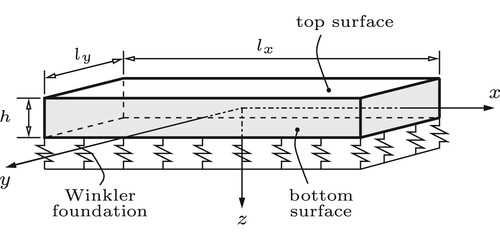
Temperature measurements refer to a concrete pavement slab at kilometre 21 of the Austrian highway ‘A2 – Süd Autobahn’. The thickness h of the slab amounted to $0.25\mathrm{m}$, see Table 1 for the geometric dimensions of the slab and the material properties of the concrete.¹ A Cartesian coordinate system is introduced. Its origin is located at the centre of gravity of the plate, see Figure 1(c). The z-axis points in the thickness direction and is oriented downwards.

Figure 1. Field testing site: (a) cuts hosting the temperature sensors and their cables, (b) condition after closing the cuts with a resin, and (c) vertical positions of the sensors.

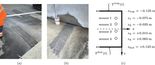
Table 1. Geometric dimensions of the studied pavement slab and material properties of concrete; values taken from Wang et al. (2019a) are estimates from multiscale modelling, accounting for corresponding properties of cement paste and aggregates.

Property	Value	Source
Length of the slab	$l_x=5.50\mathrm{m}$
Width of the slab	$l_y=2.70\mathrm{m}$
Thickness of the slab	$h=0.25\mathrm{m}$
Thermal diffusivity	$a=1.4\times {10}^{-6}{\mathrm{m}}^2/\mathrm{s}$	Equation (13(13) $a=1.4\times {10}^{-6}{\mathrm{m}}^2/\mathrm{s}.$(13) )
Coefficient of thermal expansion	${\alpha }_T=1.153\times {10}^{-5}{/}^{\circ }\mathrm{C}$	(Wang et al. 2019a)
Modulus of elasticity	$E=31.76\mathrm{GPa}$	(Wang et al. 2019a)
Poisson's ratio	$\nu =0.203$	(Wang et al. 2019a)
Mass density	$\rho =2,400\mathrm{kg}/{\mathrm{m}}^3$

The slab was equipped with four industrial standard-type temperature sensors ‘PT100A’. As for their installation, the slab was cut with a diamond-tooth saw, see Figure 1 (a). The sensors were positioned at depths amounting to 5 cm, 9 cm, 14 cm, and 19 cm. The corresponding z-coordinates read as $z_1=-0.075\mathrm{m}$, $z_2=-0.035\mathrm{m}$, $z_3=+0.015\mathrm{m}$, and $z_4=+0.065\mathrm{m}$. After placement of the sensors, the 10 mm wide cuts were closed using the resin ‘Roadplast’, see Figure 1(b). Given that the cuts are rather thin, it is assumed that the influence of the resin on the temperature distribution in the studied slab is insignificant.

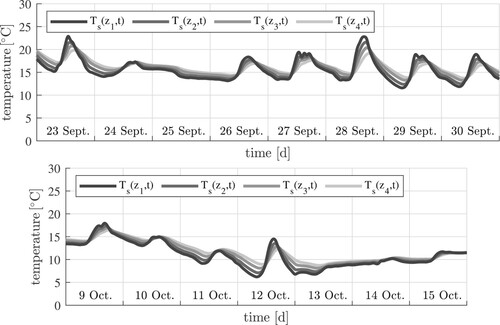
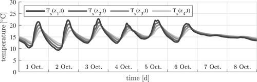
The temperatures were recorded once every hour, from 00:00 on 23 Sept. to 24:00 on 15 Oct. This resulted in 552 sets of four temperature measurements. Splines are used for temporal interpolation between the measured values, see Figure 2. These splines are denoted as $T_s(z_1,t)$, $T_s(z_2,t)$, $T_s(z_3,t)$ and $T_s(z_4,t)$.

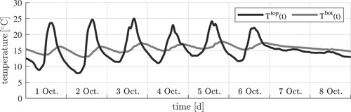
Figure 2. Temperatures measured $5\mathrm{cm}$, $9\mathrm{cm}$, $14\mathrm{cm}$ and $19\mathrm{cm}$ underneath the top surface, from 1 Oct. to 8 Oct.; for the complete database, see Appendix 2; both 7 and 8 Oct. were foggy days with a quite stable temperature, see (Time 2020).

2.2. Statement of the transient heat conduction problem

Heat conduction is a boundary value problem. The field equation is the heat equation. Focusing on one-dimensional heat conduction in the thickness direction, it reads as (1) $\frac{\mathrm{\partial }T(z,t)}{\mathrm{\partial }t}=a\frac{{\mathrm{\partial }}^{2}T(z,t)}{\mathrm{\partial }{z}^2},$(1) where T denotes the temperature, a the thermal diffusivity of concrete, and t the time variable. 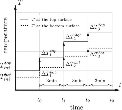As the initial condition, a linear temperature distribution is introduced: (2) $T(z,t=0)=\frac{T_{ini}^{bot}+T_{ini}^{top}}{2}+[T_{ini}^{bot}-T_{ini}^{top}]\frac{z}{h},$(2) with $T_{ini}^{top}$ and $T_{ini}^{bot}$ denoting the initial temperature at the top and at the bottom of the plate, respectively. As for the boundary conditions, temperature histories $T^{top}(t)$ and $T^{bot}(t)$ will be prescribed at the top and the bottom of the plate, respectively. As the basis for an analytical series solution, $T^{top}(t)$ and $T^{bot}(t)$ are represented as a sequence of temperature steps. The latter are described by means of the Heaviside function $H(t-t_i)$. It is equal to 0 for $t<t_i$ and equal to 1 for $t\ge t_i$: (3) $T\left(z=-\frac{h}{2},t\right)=T_{ini}^{top}+\sum _{i=1}^{N_i}\mathrm{\Delta }{T}_i^{top}H(t-t_i),$(3) (4) $T\left(z=+\frac{h}{2},t\right)=T_{ini}^{bot}+\sum _{i=1}^{N_i}\mathrm{\Delta }{T}_i^{bot}H(t-t_i),$(4) where $N_i$ denotes the number of considered temperature steps. $\mathrm{\Delta }{T}_i^{top}$ and $\mathrm{\Delta }{T}_i^{bot}$ stand for the $i^{\mathrm{th}}$ temperature steps at the top and the bottom surface, respectively. They result from the temperature histories as (5) $\mathrm{\Delta }{T}_i^{top}=T^{top}(t_i)-T^{top}(t_{i-1}),$(5) (6) $\mathrm{\Delta }{T}_i^{bot}=T^{bot}(t_i)-T^{bot}(t_{i-1}),$(6)

with $T^{top}(t_0)=T_{ini}^{top}$ and $T^{bot}(t_0)=T_{ini}^{bot}$, see also Figure 3. Temperature steps will be prescribed every three minutes. This requires temporal interpolation and spatial extrapolation of temperature measurements.

Figure 3. Representation of the temperature histories at the top and the bottom of the plate by means of step functions, starting from the initial temperatures $T_{ini}^{top}$ and $T_{ini}^{bot}$, respectively.

As for temporal interpolation between temperature measurements, the aforementioned splines (index s) are used, see Figure 2. They are evaluated every three minutes. This yields 11,040 sets of four temperature values referring to 11,040 different instants of time and to four different depths. Every set of four values is the basis for extrapolating the temperature vertically both to the top and the bottom of the plate. Following many examples (Choubane and Tia 1992; Mohamed and Hansen 1997; Ioannides and Khazanovich 1998; Khazanovich et al. 2001; Zhang et al. 2003; Hiller and Roesler 2010), one best-fit quadratic polynomial is employed at every time instant t: (7) $T(z,t)=A_0(t)+A_1(t)\cdot \frac{z}{h}+A_2(t)\cdot {\left(\frac{z}{h}\right)}^2,$(7) see also Figure 4. The $11,040$ sets of coefficients $A_0(t)$, $A_1(t)$, and $A_2(t)$ are functions of the temperatures prevailing at time t in the four different depths, see Table 2.

Figure 4. Spatial extrapolation of temperatures referring to the positions of the four PT100A sensors, see the circles, to the top and the bottom of the plate, see the squares, using the best-fit quadratic polynomial according to Equation (7(7) $T(z,t)=A_0(t)+A_1(t)\cdot \frac{z}{h}+A_2(t)\cdot {\left(\frac{z}{h}\right)}^2,$(7) ), see also Table 2.

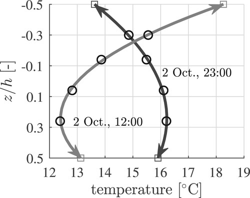
Table 2. Coordinates of the sensors and of the top and the bottom of the slab; thickness of the slab; optimal coefficients of best-fit quadratic polynomials (7(7) $T(z,t)=A_0(t)+A_1(t)\cdot \frac{z}{h}+A_2(t)\cdot {\left(\frac{z}{h}\right)}^2,$(7) ); and resulting extrapolation formulae for quantification of the temperature at the top and the bottom of the plate.

z-coordinates of the sensors, the top and the bottom of the slab, and its thickness
$z_1=-0.075\mathrm{m}$, $z_2=-0.035\mathrm{m}$, $z_3=+0.015\mathrm{m}$, $z_4=+0.065\mathrm{m}$
$z_{top}=-0.125\mathrm{m}$, $z_{bot}=+0.125\mathrm{m}$; $h=0.25\mathrm{m}$
Optimal coefficients of the quadratic fitting function (7(7) $T(z,t)=A_0(t)+A_1(t)\cdot \frac{z}{h}+A_2(t)\cdot {\left(\frac{z}{h}\right)}^2,$(7) )
$A_0(t)=-0.12592T_s(z_1,t)+0.51231T_s(z_2,t)+0.62795T_s(z_3,t)-0.01434T_s(z_4,t)$
$A_1(t)=-1.24783T_s(z_1,t)-0.85548T_s(z_2,t)+0.20487T_s(z_3,t)+1.89844T_s(z_4,t)$
$A_2(t)=+7.48851T_s(z_1,t)-6.37106T_s(z_2,t)-8.22573T_s(z_3,t)+7.10827T_s(z_4,t)$
Formulae providing spatial extrapolation of temperatures to the top and the bottom of the plate
$T^{top}(t)=T(z_{top},t)=+2.37013T_s(z_1,t)-0.65272T_s(z_2,t)-1.53092T_s(z_3,t)+0.81351T_s(z_4,t)$
$T^{bot}(t)=T(z_{bot},t)=+1.12230T_s(z_1,t)-1.50819T_s(z_2,t)-1.32605T_s(z_3,t)+2.71194T_s(z_4,t)$

The quadratic correlation coefficient amounts on average to $R^2=0.95$. Closed-form solutions for the temperatures at the top and the bottom of the plate, as functions of the temperatures in the four different depths of the sensors, are also given in Table 2. The obtained surface temperature histories are exemplarily illustrated in Figure 5. The largest change of temperature within one day occurred on 2 Oct. at the top surface: the minimum temperature amounted to ${7.8}^{\circ }\mathrm{C}$, the maximum temperature to ${24.7}^{\circ }\mathrm{C}$. The determined and prescribed surface temperature histories implicitly account for the ambient climatic conditions, such as the air temperature, the solar radiation, and the wind velocity.

Figure 5. Boundary conditions of the transient heat conduction problem: evolution of temperatures at the top and the bottom of the plate, obtained with the extrapolation function (7(7) $T(z,t)=A_0(t)+A_1(t)\cdot \frac{z}{h}+A_2(t)\cdot {\left(\frac{z}{h}\right)}^2,$(7) ); the data shown refer to 1 Oct. to 8 Oct.

2.3. Solution of the transient heat conduction problem

The solution to the heat equation for variable temperature at the top of the plate and constant temperature at the bottom, documented in Wang et al. (2019a), is extended towards consideration of temperature steps at the top and the bottom surface. This extended solution reads as (8) $\begin{array}{rl}T(z,t)& =\frac{T^{bot}(t)+T^{top}(t)}{2}+[T^{bot}(t)-T^{top}(t)]\frac{z}{h}\\ & -\sum _{i=1}^{N_i}(\mathrm{\Delta }{T}_i^{top}-\mathrm{\Delta }{T}_i^{bot})\sum _{n=1}^{\mathrm{\infty }}\frac{(-1{)}^n}{n\pi }\sin \left(\frac{2n\pi z}{h}\right)\\ & \exp (-(2n\pi {)}^2\frac{a⟨t-t_i⟩}{h^2})+\sum _{i=1}^{N_i}(\mathrm{\Delta }{T}_i^{top}+\mathrm{\Delta }{T}_i^{bot})\\ & \sum _{n=1}^{\mathrm{\infty }}\frac{2(-1{)}^n}{(2n-1)\pi }\cos \left(\frac{(2n-1)\pi z}{h}\right)\\ & \exp (-(2n-1{)}^2{\pi }^2\frac{a⟨t-t_i⟩}{h^2}),\end{array}$(8) where the angled brackets denote the Macaulay operator $⟨t-t_i⟩=(t-t_i+|t-t_i|)/2$.

The infinite sums in Equation (8(8) $\begin{array}{rl}T(z,t)& =\frac{T^{bot}(t)+T^{top}(t)}{2}+[T^{bot}(t)-T^{top}(t)]\frac{z}{h}\\ & -\sum _{i=1}^{N_i}(\mathrm{\Delta }{T}_i^{top}-\mathrm{\Delta }{T}_i^{bot})\sum _{n=1}^{\mathrm{\infty }}\frac{(-1{)}^n}{n\pi }\sin \left(\frac{2n\pi z}{h}\right)\\ & \exp (-(2n\pi {)}^2\frac{a⟨t-t_i⟩}{h^2})+\sum _{i=1}^{N_i}(\mathrm{\Delta }{T}_i^{top}+\mathrm{\Delta }{T}_i^{bot})\\ & \sum _{n=1}^{\mathrm{\infty }}\frac{2(-1{)}^n}{(2n-1)\pi }\cos \left(\frac{(2n-1)\pi z}{h}\right)\\ & \exp (-(2n-1{)}^2{\pi }^2\frac{a⟨t-t_i⟩}{h^2}),\end{array}$(8) ) must be truncated. In order to ensure a well-converged solution, the exponential functions in Equation (8(8) $\begin{array}{rl}T(z,t)& =\frac{T^{bot}(t)+T^{top}(t)}{2}+[T^{bot}(t)-T^{top}(t)]\frac{z}{h}\\ & -\sum _{i=1}^{N_i}(\mathrm{\Delta }{T}_i^{top}-\mathrm{\Delta }{T}_i^{bot})\sum _{n=1}^{\mathrm{\infty }}\frac{(-1{)}^n}{n\pi }\sin \left(\frac{2n\pi z}{h}\right)\\ & \exp (-(2n\pi {)}^2\frac{a⟨t-t_i⟩}{h^2})+\sum _{i=1}^{N_i}(\mathrm{\Delta }{T}_i^{top}+\mathrm{\Delta }{T}_i^{bot})\\ & \sum _{n=1}^{\mathrm{\infty }}\frac{2(-1{)}^n}{(2n-1)\pi }\cos \left(\frac{(2n-1)\pi z}{h}\right)\\ & \exp (-(2n-1{)}^2{\pi }^2\frac{a⟨t-t_i⟩}{h^2}),\end{array}$(8) ) are analysed. Their values decrease with increasing values of both n and $⟨t-t_i⟩$. Evaluated for the same values of n and $⟨t-t_i⟩$, the exponential function containing $(2n-1{)}^2{\pi }^2$ is larger than the one containing $(2n\pi {)}^2$. Thus, the following discussion is focused on the former exponential function. Summands of the infinite sums in Equation (8(8) $\begin{array}{rl}T(z,t)& =\frac{T^{bot}(t)+T^{top}(t)}{2}+[T^{bot}(t)-T^{top}(t)]\frac{z}{h}\\ & -\sum _{i=1}^{N_i}(\mathrm{\Delta }{T}_i^{top}-\mathrm{\Delta }{T}_i^{bot})\sum _{n=1}^{\mathrm{\infty }}\frac{(-1{)}^n}{n\pi }\sin \left(\frac{2n\pi z}{h}\right)\\ & \exp (-(2n\pi {)}^2\frac{a⟨t-t_i⟩}{h^2})+\sum _{i=1}^{N_i}(\mathrm{\Delta }{T}_i^{top}+\mathrm{\Delta }{T}_i^{bot})\\ & \sum _{n=1}^{\mathrm{\infty }}\frac{2(-1{)}^n}{(2n-1)\pi }\cos \left(\frac{(2n-1)\pi z}{h}\right)\\ & \exp (-(2n-1{)}^2{\pi }^2\frac{a⟨t-t_i⟩}{h^2}),\end{array}$(8) ) are significant only if the values of the described exponential functions are larger than or equal to a small tolerance value tol which is set equal to $1\times {10}^{-4}$: (9) $\exp (-(2n-1{)}^2{\pi }^2\frac{a⟨t-t_i⟩}{h^2})\ge tol.$(9) Solving condition (9(9) $\exp (-(2n-1{)}^2{\pi }^2\frac{a⟨t-t_i⟩}{h^2})\ge tol.$(9) ) for n yields: (10) $n\le \frac{1}{2}[1+\sqrt{-\frac{\ln (tol)h^2}{{\pi }^{2}a⟨t-t_i⟩}}].$(10) The number of significant summands n according to Equation (10(10) $n\le \frac{1}{2}[1+\sqrt{-\frac{\ln (tol)h^2}{{\pi }^{2}a⟨t-t_i⟩}}].$(10) ) increases as $⟨t-t_i⟩$ decreases. Herein, the smallest value of $⟨t-t_i⟩$ amounts to three minutes. This value yields the largest number of n.

The number of significant summands n according to inequality (10(10) $n\le \frac{1}{2}[1+\sqrt{-\frac{\ln (tol)h^2}{{\pi }^{2}a⟨t-t_i⟩}}].$(10) ) decreases with increasing period of time $⟨t-t_i⟩$. This provides the motivation to determine the value of $⟨t-t_i⟩$ for which one summand remains to be significant. Thus, n is set equal to 1 and the resulting inequality (10(10) $n\le \frac{1}{2}[1+\sqrt{-\frac{\ln (tol)h^2}{{\pi }^{2}a⟨t-t_i⟩}}].$(10) ) is solved for $⟨t-t_i⟩$. This yields (11) $⟨t-t_i⟩\le -\frac{h^2\ln (tol)}{a{\pi }^2}.$(11) Temperature steps that have occurred in a temporal distance larger than the right-hand-side of inequality (11(11) $⟨t-t_i⟩\le -\frac{h^2\ln (tol)}{a{\pi }^2}.$(11) ) do not influence the temperature distribution at time t significantly.

2.4. Quantification of the thermal diffusivity of concrete

The numerical evaluation of the inequalities (10(10) $n\le \frac{1}{2}[1+\sqrt{-\frac{\ln (tol)h^2}{{\pi }^{2}a⟨t-t_i⟩}}].$(10) ) and (11(11) $⟨t-t_i⟩\le -\frac{h^2\ln (tol)}{a{\pi }^2}.$(11) ) requires a numerical value for the thermal diffusivity a. The heat Equation (1(1) $\frac{\mathrm{\partial }T(z,t)}{\mathrm{\partial }t}=a\frac{{\mathrm{\partial }}^{2}T(z,t)}{\mathrm{\partial }{z}^2},$(1) ) clarifies that identification of a requires transient heat conduction, implying that the temperature must change with time. The most significant of these changes were recorded on 2 Oct., see Figure 2. Therefore, a will be identified such that the simulation of the transient heat conduction problem reproduces temperature measurements recorded on 2 Oct. in a best-possible fashion.

The search interval for the thermal diffusivity is introduced as $a\in [1.0,2.0]\times {10}^{-6}{\mathrm{m}}^2/\mathrm{s}$. Inserting the smallest of these values, $a=1.0\times {10}^{-6}{\mathrm{m}}^2/\mathrm{s}$, together with $tol=1\times {10}^{-4}$, $⟨t-t_i⟩=180\mathrm{s}$, and $h=0.25\mathrm{m}$ into inequality (10(10) $n\le \frac{1}{2}[1+\sqrt{-\frac{\ln (tol)h^2}{{\pi }^{2}a⟨t-t_i⟩}}].$(10) ) yields $n\le 9.5$. Thus, the infinite sums in Equation (8(8) $\begin{array}{rl}T(z,t)& =\frac{T^{bot}(t)+T^{top}(t)}{2}+[T^{bot}(t)-T^{top}(t)]\frac{z}{h}\\ & -\sum _{i=1}^{N_i}(\mathrm{\Delta }{T}_i^{top}-\mathrm{\Delta }{T}_i^{bot})\sum _{n=1}^{\mathrm{\infty }}\frac{(-1{)}^n}{n\pi }\sin \left(\frac{2n\pi z}{h}\right)\\ & \exp (-(2n\pi {)}^2\frac{a⟨t-t_i⟩}{h^2})+\sum _{i=1}^{N_i}(\mathrm{\Delta }{T}_i^{top}+\mathrm{\Delta }{T}_i^{bot})\\ & \sum _{n=1}^{\mathrm{\infty }}\frac{2(-1{)}^n}{(2n-1)\pi }\cos \left(\frac{(2n-1)\pi z}{h}\right)\\ & \exp (-(2n-1{)}^2{\pi }^2\frac{a⟨t-t_i⟩}{h^2}),\end{array}$(8) ) are truncated after the first nine terms. Inserting the same values of a, tol, and h into inequality (11(11) $⟨t-t_i⟩\le -\frac{h^2\ln (tol)}{a{\pi }^2}.$(11) ) yields $⟨t-t_i⟩\le 16.2\mathrm{h}$. Thus, in order to obtain a reliable temperature solution at 00:00 on 2 Oct., the simulation must start 16.2 hours earlier. For the sake of simplicity, the simulation is started 24 hours earlier. The corresponding temperatures at the top and the bottom of the plate, see 00:00 on 1 Oct. in Figure 5, serve as initial values, i.e. $T_{ini}^{top}={12.5}^{\circ }\mathrm{C}$ and $T_{ini}^{bot}={15.4}^{\circ }\mathrm{C}$. Temperature steps are prescribed every three minutes. They are computed based on Equations (5(5) $\mathrm{\Delta }{T}_i^{top}=T^{top}(t_i)-T^{top}(t_{i-1}),$(5) ) and (6(6) $\mathrm{\Delta }{T}_i^{bot}=T^{bot}(t_i)-T^{bot}(t_{i-1}),$(6) ) and Table 2. Given that the simulation covers 48 hours, index i in Equation (8(8) $\begin{array}{rl}T(z,t)& =\frac{T^{bot}(t)+T^{top}(t)}{2}+[T^{bot}(t)-T^{top}(t)]\frac{z}{h}\\ & -\sum _{i=1}^{N_i}(\mathrm{\Delta }{T}_i^{top}-\mathrm{\Delta }{T}_i^{bot})\sum _{n=1}^{\mathrm{\infty }}\frac{(-1{)}^n}{n\pi }\sin \left(\frac{2n\pi z}{h}\right)\\ & \exp (-(2n\pi {)}^2\frac{a⟨t-t_i⟩}{h^2})+\sum _{i=1}^{N_i}(\mathrm{\Delta }{T}_i^{top}+\mathrm{\Delta }{T}_i^{bot})\\ & \sum _{n=1}^{\mathrm{\infty }}\frac{2(-1{)}^n}{(2n-1)\pi }\cos \left(\frac{(2n-1)\pi z}{h}\right)\\ & \exp (-(2n-1{)}^2{\pi }^2\frac{a⟨t-t_i⟩}{h^2}),\end{array}$(8) ) runs from 1 to 960.

The search interval of a is subdivided into 40 equidistant values. For each one of them, Equation (8(8) $\begin{array}{rl}T(z,t)& =\frac{T^{bot}(t)+T^{top}(t)}{2}+[T^{bot}(t)-T^{top}(t)]\frac{z}{h}\\ & -\sum _{i=1}^{N_i}(\mathrm{\Delta }{T}_i^{top}-\mathrm{\Delta }{T}_i^{bot})\sum _{n=1}^{\mathrm{\infty }}\frac{(-1{)}^n}{n\pi }\sin \left(\frac{2n\pi z}{h}\right)\\ & \exp (-(2n\pi {)}^2\frac{a⟨t-t_i⟩}{h^2})+\sum _{i=1}^{N_i}(\mathrm{\Delta }{T}_i^{top}+\mathrm{\Delta }{T}_i^{bot})\\ & \sum _{n=1}^{\mathrm{\infty }}\frac{2(-1{)}^n}{(2n-1)\pi }\cos \left(\frac{(2n-1)\pi z}{h}\right)\\ & \exp (-(2n-1{)}^2{\pi }^2\frac{a⟨t-t_i⟩}{h^2}),\end{array}$(8) ) is used to compute the evolution of the temperature field from 00:00 to 24:00 on 2 Oct. The simulated temperature fields are denoted as $T(z,t,a)$. In order to quantify the quality of reproduction of the 24 measurements (index m) of each one of the four temperature sensors (indexes s = 1, 2, 3, 4), the root mean square error (RMSE) between computed and measured temperatures is minimised:

(12) $RMSE(a)=\sqrt{\frac{1}{4\times 24}\sum _{s=1}^4\sum _{m=1}^{24}[T(z_s,t_m,a)-T_{exp}(z_s,t_m){]}^2}\to min,$(12) where $T_{\exp }(z_s,t_m)$ denotes the temperature measurements. The optimal value of a is obtained as (13) $a=1.4\times {10}^{-6}{\mathrm{m}}^2/\mathrm{s}.$(13) Notably, a according to Equation (13(13) $a=1.4\times {10}^{-6}{\mathrm{m}}^2/\mathrm{s}.$(13) ) is within the expected range of values as reported by Neville (1995): $a\in [0.6\times {10}^{-6}1.6\times {10}^{-6}]{\mathrm{m}}^2$/s. The corresponding minimum of $RMSE(a)$ amounts to ${0.4}^{\circ }\mathrm{C}$. Simulated temperatures reproduce the measurements in a satisfactory fashion, see Figure 6.

Figure 6. Temperature profiles referring to 2 Oct.: the circles label measured temperatures, the solid lines refer to the solution of the heat conduction problem according to Equation (8(8) $\begin{array}{rl}T(z,t)& =\frac{T^{bot}(t)+T^{top}(t)}{2}+[T^{bot}(t)-T^{top}(t)]\frac{z}{h}\\ & -\sum _{i=1}^{N_i}(\mathrm{\Delta }{T}_i^{top}-\mathrm{\Delta }{T}_i^{bot})\sum _{n=1}^{\mathrm{\infty }}\frac{(-1{)}^n}{n\pi }\sin \left(\frac{2n\pi z}{h}\right)\\ & \exp (-(2n\pi {)}^2\frac{a⟨t-t_i⟩}{h^2})+\sum _{i=1}^{N_i}(\mathrm{\Delta }{T}_i^{top}+\mathrm{\Delta }{T}_i^{bot})\\ & \sum _{n=1}^{\mathrm{\infty }}\frac{2(-1{)}^n}{(2n-1)\pi }\cos \left(\frac{(2n-1)\pi z}{h}\right)\\ & \exp (-(2n-1{)}^2{\pi }^2\frac{a⟨t-t_i⟩}{h^2}),\end{array}$(8) ), using the surface temperature histories of Figure 5 as boundary conditions.

2.5. Solution of the heat conduction problem throughout the entire monitoring period

Inserting a according to Equation (13(13) $a=1.4\times {10}^{-6}{\mathrm{m}}^2/\mathrm{s}.$(13) ), $tol=1\times {10}^{-4}$, $⟨t-t_i⟩=180\mathrm{s}$, and $h=0.25\mathrm{m}$ into inequality (10(10) $n\le \frac{1}{2}[1+\sqrt{-\frac{\ln (tol)h^2}{{\pi }^{2}a⟨t-t_i⟩}}].$(10) ) yields $n\le 8.1$. Thus, the infinite sums in Equation (8(8) $\begin{array}{rl}T(z,t)& =\frac{T^{bot}(t)+T^{top}(t)}{2}+[T^{bot}(t)-T^{top}(t)]\frac{z}{h}\\ & -\sum _{i=1}^{N_i}(\mathrm{\Delta }{T}_i^{top}-\mathrm{\Delta }{T}_i^{bot})\sum _{n=1}^{\mathrm{\infty }}\frac{(-1{)}^n}{n\pi }\sin \left(\frac{2n\pi z}{h}\right)\\ & \exp (-(2n\pi {)}^2\frac{a⟨t-t_i⟩}{h^2})+\sum _{i=1}^{N_i}(\mathrm{\Delta }{T}_i^{top}+\mathrm{\Delta }{T}_i^{bot})\\ & \sum _{n=1}^{\mathrm{\infty }}\frac{2(-1{)}^n}{(2n-1)\pi }\cos \left(\frac{(2n-1)\pi z}{h}\right)\\ & \exp (-(2n-1{)}^2{\pi }^2\frac{a⟨t-t_i⟩}{h^2}),\end{array}$(8) ) are truncated after the first eight terms. Inserting the same values of a, tol, and h into inequality (11(11) $⟨t-t_i⟩\le -\frac{h^2\ln (tol)}{a{\pi }^2}.$(11) ) yields $⟨t-t_i⟩\le 11.6\mathrm{h}$. Therefore, the temperature solution becomes reliable some 12 hours after the start of the simulation at 00:00 on 23 Sept. The corresponding temperatures at the top and the bottom of the plate serve as initial values, i.e. $T_{ini}^{top}={16.4}^{\circ }\mathrm{C}$ and $T_{ini}^{bot}={19.6}^{\circ }\mathrm{C}$. Temperature steps are prescribed every three minutes. They are computed based on Equations (5(5) $\mathrm{\Delta }{T}_i^{top}=T^{top}(t_i)-T^{top}(t_{i-1}),$(5) ) and (6(6) $\mathrm{\Delta }{T}_i^{bot}=T^{bot}(t_i)-T^{bot}(t_{i-1}),$(6) ) and Table 2. Given that the simulation covers 23 days, index i in Equation (8(8) $\begin{array}{rl}T(z,t)& =\frac{T^{bot}(t)+T^{top}(t)}{2}+[T^{bot}(t)-T^{top}(t)]\frac{z}{h}\\ & -\sum _{i=1}^{N_i}(\mathrm{\Delta }{T}_i^{top}-\mathrm{\Delta }{T}_i^{bot})\sum _{n=1}^{\mathrm{\infty }}\frac{(-1{)}^n}{n\pi }\sin \left(\frac{2n\pi z}{h}\right)\\ & \exp (-(2n\pi {)}^2\frac{a⟨t-t_i⟩}{h^2})+\sum _{i=1}^{N_i}(\mathrm{\Delta }{T}_i^{top}+\mathrm{\Delta }{T}_i^{bot})\\ & \sum _{n=1}^{\mathrm{\infty }}\frac{2(-1{)}^n}{(2n-1)\pi }\cos \left(\frac{(2n-1)\pi z}{h}\right)\\ & \exp (-(2n-1{)}^2{\pi }^2\frac{a⟨t-t_i⟩}{h^2}),\end{array}$(8) ) runs from 1 to 11,040.

The quality of the reproduction of 540 measurements, from 12:00 on 23 Sept. to 24:00 on 15 Oct., is quantified by means of the root mean square errors (RMSE) between computed and measured temperatures: (14) $RMSE=\sqrt{\frac{1}{4\times 540}\sum _{s=1}^4\sum _{m=1}^{540}[T(z_s,t_m)-T_{exp}(z_s,t_m){]}^2}={0.3}^{\circ }\mathrm{C}.$(14) This very satisfactory result corroborates the value of the thermal diffusivity given in Equation (13(13) $a=1.4\times {10}^{-6}{\mathrm{m}}^2/\mathrm{s}.$(13) ). The solution of the heat conduction problem serves as the basis for the thermo-mechanical analysis of thermal stresses.

3. Thermo-mechanical analysis of thermal stresses

3.1. Decomposition of thermal eigenstrains as the basis for quantification of thermal stresses

Thermal eigenstrains ${\epsilon }_{xx}^e$, ${\epsilon }_{yy}^e$ and ${\epsilon }_{zz}^e$ are equal to the coefficient of thermal expansion, ${\alpha }_T=1.153\times {10}^{-5}{/}^{\circ }\mathrm{C}$, see (Wang et al. 2019a), multiplied with the temperature change, $\mathrm{\Delta }T(z,t)$, (15) ${\epsilon }_{xx}^e(z,t)={\epsilon }_{yy}^e(z,t)={\epsilon }_{zz}^e(z,t)={\alpha }_T\mathrm{\Delta }T(z,t),$(15) with (16) $\mathrm{\Delta }T(z,t)=T(z,t)-T_{ref},$(16) where $T_{ref}$ denotes the reference temperature at which the plate is free of thermal strains. $T_{ref}$ is usually related to the temperature at which the concrete slab sets (NCHRP 2004). As the temperature sensors were installed in an existing pavement slab for which $T_{ref}$ was not documented, the reference temperature is estimated as $T_{ref}={17}^{\circ }$C.

The thermal eigenstrains, according to Equations (15(15) ${\epsilon }_{xx}^e(z,t)={\epsilon }_{yy}^e(z,t)={\epsilon }_{zz}^e(z,t)={\alpha }_T\mathrm{\Delta }T(z,t),$(15) ) and (16(16) $\mathrm{\Delta }T(z,t)=T(z,t)-T_{ref},$(16) ) are spatially nonlinear along the thickness direction, because transient heat conduction goes along with spatially nonlinear temperature distributions, see also Equation (8(8) $\begin{array}{rl}T(z,t)& =\frac{T^{bot}(t)+T^{top}(t)}{2}+[T^{bot}(t)-T^{top}(t)]\frac{z}{h}\\ & -\sum _{i=1}^{N_i}(\mathrm{\Delta }{T}_i^{top}-\mathrm{\Delta }{T}_i^{bot})\sum _{n=1}^{\mathrm{\infty }}\frac{(-1{)}^n}{n\pi }\sin \left(\frac{2n\pi z}{h}\right)\\ & \exp (-(2n\pi {)}^2\frac{a⟨t-t_i⟩}{h^2})+\sum _{i=1}^{N_i}(\mathrm{\Delta }{T}_i^{top}+\mathrm{\Delta }{T}_i^{bot})\\ & \sum _{n=1}^{\mathrm{\infty }}\frac{2(-1{)}^n}{(2n-1)\pi }\cos \left(\frac{(2n-1)\pi z}{h}\right)\\ & \exp (-(2n-1{)}^2{\pi }^2\frac{a⟨t-t_i⟩}{h^2}),\end{array}$(8) ) and Figure 6. The structural behaviour of thin plates suggests to decompose the eigenstrains, at any time instant t, into three parts: the eigenstretch of the plate, its eigencurvature, and the eigendistortions of the generators of the plate (Wang et al. 2019a). Rules for this decomposition follow from the Kirchhoff-Love hypothesis, see Appendix 1. The eigenstretch of the plate reads as (17) ${\epsilon }^e(t)=\frac{1}{h}\underset{-\frac{h}{2}}{\overset{+\frac{h}{2}}{\int }}{\alpha }_T\mathrm{\Delta }T(z,t)\mathrm{d}z,$(17) and its eigencurvature as (18) ${\kappa }^e(t)=\frac{12}{h^3}\underset{-\frac{h}{2}}{\overset{+\frac{h}{2}}{\int }}{\alpha }_T\mathrm{\Delta }T(z,t)\cdot z\mathrm{d}z.$(18) Subtracting from the thermal eigenstrains, ${\alpha }_T\mathrm{\Delta }T(z,t)$, the constant part representing the eigenstretch of the plate, ${\epsilon }^e(t)$, and the linear part related to its eigencurvature, ${\kappa }^e(t)\cdot z$, yields the spatially nonlinear eigendistortions of the generators of the plate (19) ${\epsilon }_{dist}^e(z,t)={\alpha }_T\mathrm{\Delta }T(z,t)-{\epsilon }^e(t)-{\kappa }^e(t)\cdot z,$(19) see also Figure 7. Analytical expressions for ${\epsilon }^e(t)$, ${\kappa }^e(t)$ and ${\epsilon }_{dist}^e(z,t)$, according to Equations (15(15) ${\epsilon }_{xx}^e(z,t)={\epsilon }_{yy}^e(z,t)={\epsilon }_{zz}^e(z,t)={\alpha }_T\mathrm{\Delta }T(z,t),$(15) )–(19(19) ${\epsilon }_{dist}^e(z,t)={\alpha }_T\mathrm{\Delta }T(z,t)-{\epsilon }^e(t)-{\kappa }^e(t)\cdot z,$(19) ), obtained for temperature profiles representing solutions of the heat equation, see Equation (8(8) $\begin{array}{rl}T(z,t)& =\frac{T^{bot}(t)+T^{top}(t)}{2}+[T^{bot}(t)-T^{top}(t)]\frac{z}{h}\\ & -\sum _{i=1}^{N_i}(\mathrm{\Delta }{T}_i^{top}-\mathrm{\Delta }{T}_i^{bot})\sum _{n=1}^{\mathrm{\infty }}\frac{(-1{)}^n}{n\pi }\sin \left(\frac{2n\pi z}{h}\right)\\ & \exp (-(2n\pi {)}^2\frac{a⟨t-t_i⟩}{h^2})+\sum _{i=1}^{N_i}(\mathrm{\Delta }{T}_i^{top}+\mathrm{\Delta }{T}_i^{bot})\\ & \sum _{n=1}^{\mathrm{\infty }}\frac{2(-1{)}^n}{(2n-1)\pi }\cos \left(\frac{(2n-1)\pi z}{h}\right)\\ & \exp (-(2n-1{)}^2{\pi }^2\frac{a⟨t-t_i⟩}{h^2}),\end{array}$(8) ), are listed in Table 3. Numerical results obtained for 2 Oct. are illustrated in Figure 8.

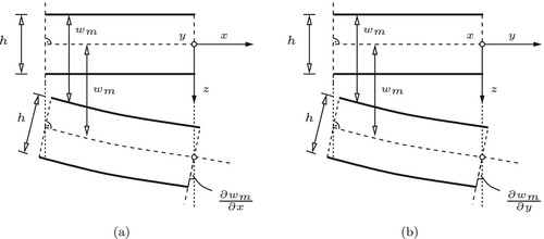
Figure 7. Decomposition of thermal eigenstrains into (i) a spatially constant part, ${\epsilon }^e$, equal to the eigenstretch of the plate, (ii) a spatially linear part, ${\kappa }^e\cdot z$, related to the eigencurvature of the plate, and (iii) the spatially nonlinear rest, representing the eigendistortion ${\epsilon }_{dist}^e$ of the generators of the plate.

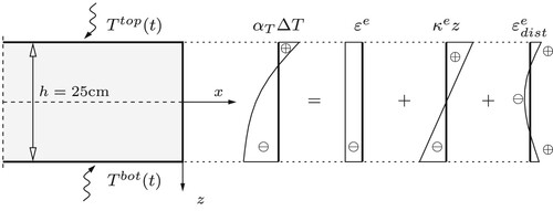
Figure 8. Exemplary results of thermo-elastic analysis: Decomposition of (a) the thermal eigenstrains into (b) eigenstrains referring to eigenstretches ${\epsilon }^e$ of the plate, (c) eigenstrains referring to eigencurvatures ${\kappa }^e$ of the plate (these eigenstrains are equal to the product of eigencurvatures ${\kappa }^e$ and the z-coordinate), and (d) eigenstrains referring to eigendistortions ${\epsilon }_{dist}^e$ of the generators of the plate; the results have shown refer to 2 Oct.

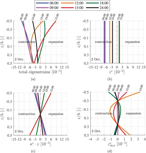
Table 3. Expressions for eigenstretches and eigencurvatures of the plate and for the eigendistortion of the generators of the plate, obtained from inserting the solution of the heat equation according to Equation (8(8) $\begin{array}{rl}T(z,t)& =\frac{T^{bot}(t)+T^{top}(t)}{2}+[T^{bot}(t)-T^{top}(t)]\frac{z}{h}\\ & -\sum _{i=1}^{N_i}(\mathrm{\Delta }{T}_i^{top}-\mathrm{\Delta }{T}_i^{bot})\sum _{n=1}^{\mathrm{\infty }}\frac{(-1{)}^n}{n\pi }\sin \left(\frac{2n\pi z}{h}\right)\\ & \exp (-(2n\pi {)}^2\frac{a⟨t-t_i⟩}{h^2})+\sum _{i=1}^{N_i}(\mathrm{\Delta }{T}_i^{top}+\mathrm{\Delta }{T}_i^{bot})\\ & \sum _{n=1}^{\mathrm{\infty }}\frac{2(-1{)}^n}{(2n-1)\pi }\cos \left(\frac{(2n-1)\pi z}{h}\right)\\ & \exp (-(2n-1{)}^2{\pi }^2\frac{a⟨t-t_i⟩}{h^2}),\end{array}$(8) ) into Equation (16(16) $\mathrm{\Delta }T(z,t)=T(z,t)-T_{ref},$(16) ), the resulting expressions into Equation (15(15) ${\epsilon }_{xx}^e(z,t)={\epsilon }_{yy}^e(z,t)={\epsilon }_{zz}^e(z,t)={\alpha }_T\mathrm{\Delta }T(z,t),$(15) ), and the obtained results into Equations (17(17) ${\epsilon }^e(t)=\frac{1}{h}\underset{-\frac{h}{2}}{\overset{+\frac{h}{2}}{\int }}{\alpha }_T\mathrm{\Delta }T(z,t)\mathrm{d}z,$(17) ), (18(18) ${\kappa }^e(t)=\frac{12}{h^3}\underset{-\frac{h}{2}}{\overset{+\frac{h}{2}}{\int }}{\alpha }_T\mathrm{\Delta }T(z,t)\cdot z\mathrm{d}z.$(18) ), and (19(19) ${\epsilon }_{dist}^e(z,t)={\alpha }_T\mathrm{\Delta }T(z,t)-{\epsilon }^e(t)-{\kappa }^e(t)\cdot z,$(19) ).

	Solution of the heat conduction problem according to Equation (8(8) $\begin{array}{rl}T(z,t)& =\frac{T^{bot}(t)+T^{top}(t)}{2}+[T^{bot}(t)-T^{top}(t)]\frac{z}{h}\\ & -\sum _{i=1}^{N_i}(\mathrm{\Delta }{T}_i^{top}-\mathrm{\Delta }{T}_i^{bot})\sum _{n=1}^{\mathrm{\infty }}\frac{(-1{)}^n}{n\pi }\sin \left(\frac{2n\pi z}{h}\right)\\ & \exp (-(2n\pi {)}^2\frac{a⟨t-t_i⟩}{h^2})+\sum _{i=1}^{N_i}(\mathrm{\Delta }{T}_i^{top}+\mathrm{\Delta }{T}_i^{bot})\\ & \sum _{n=1}^{\mathrm{\infty }}\frac{2(-1{)}^n}{(2n-1)\pi }\cos \left(\frac{(2n-1)\pi z}{h}\right)\\ & \exp (-(2n-1{)}^2{\pi }^2\frac{a⟨t-t_i⟩}{h^2}),\end{array}$(8) ),
	using the surface temperature histories of Figure 5 as boundary conditions
	$\begin{array}{cc}{\epsilon }^e(t)& ={\alpha }_T(\frac{T^{bot}(t)+T^{top}(t)}{2}-T_{ref})\\ & -\sum _{i=1}^{N_i}{\alpha }_T\left(\frac{\mathrm{\Delta }{T}_i^{bot}+\mathrm{\Delta }{T}_i^{top}}{2}\right)\sum _{n=1}^{\mathrm{\infty }}\frac{8}{(2n-1{)}^2{\pi }^2}\exp (-(2n-1{)}^2{\pi }^2\frac{a⟨t-t_i⟩}{h^2})\\ {\kappa }^e(t)& ={\displaystyle \frac{{\alpha }_T}{h}[T^{bot}(t)-T^{top}(t)]}\\ & -\sum _{i=1}^{N_i}\frac{{\alpha }_T}{h}(\mathrm{\Delta }{T}_i^{bot}-\mathrm{\Delta }{T}_i^{top})\sum _{n=1}^{\mathrm{\infty }}\frac{24}{(2n\pi {)}^2}\exp (-(2n\pi {)}^2\frac{a⟨t-t_i⟩}{h^2})\end{array}$
	${\epsilon }_{dist}^e(z,t)$ follows from insertion of ${\alpha }_T\mathrm{\Delta }T(z,t)$ according to Equations (15(15) ${\epsilon }_{xx}^e(z,t)={\epsilon }_{yy}^e(z,t)={\epsilon }_{zz}^e(z,t)={\alpha }_T\mathrm{\Delta }T(z,t),$(15) ), (16(16) $\mathrm{\Delta }T(z,t)=T(z,t)-T_{ref},$(16) ), and (8(8) $\begin{array}{rl}T(z,t)& =\frac{T^{bot}(t)+T^{top}(t)}{2}+[T^{bot}(t)-T^{top}(t)]\frac{z}{h}\\ & -\sum _{i=1}^{N_i}(\mathrm{\Delta }{T}_i^{top}-\mathrm{\Delta }{T}_i^{bot})\sum _{n=1}^{\mathrm{\infty }}\frac{(-1{)}^n}{n\pi }\sin \left(\frac{2n\pi z}{h}\right)\\ & \exp (-(2n\pi {)}^2\frac{a⟨t-t_i⟩}{h^2})+\sum _{i=1}^{N_i}(\mathrm{\Delta }{T}_i^{top}+\mathrm{\Delta }{T}_i^{bot})\\ & \sum _{n=1}^{\mathrm{\infty }}\frac{2(-1{)}^n}{(2n-1)\pi }\cos \left(\frac{(2n-1)\pi z}{h}\right)\\ & \exp (-(2n-1{)}^2{\pi }^2\frac{a⟨t-t_i⟩}{h^2}),\end{array}$(8) )
	as well as ${\epsilon }^e(t)$ and ${\kappa }^e(t)$, see the expressions above, into Equation (19(19) ${\epsilon }_{dist}^e(z,t)={\alpha }_T\mathrm{\Delta }T(z,t)-{\epsilon }^e(t)-{\kappa }^e(t)\cdot z,$(19) ).

Thermal stresses are activated, only if thermal eigenstrains are kinematically constrained or prevented (Wang et al. 2019a). In linear thermoelasticity, the normal stresses read as (20) ${\sigma }_{xx}=\frac{n_{xx}}{h}+\frac{m_{xx}}{h^3/12}z-\frac{E{\epsilon }_{dist}^e}{1-\nu },$(20) (21) ${\sigma }_{yy}=\frac{n_{yy}}{h}+\frac{m_{yy}}{h^3/12}z-\frac{E{\epsilon }_{dist}^e}{1-\nu },$(21) see Appendix 1 for the derivation. $n_{xx}$ and $n_{yy}$, denoting membrane forces per length, are activated if ${\epsilon }^e$ is constrained or prevented. $m_{xx}$ and $m_{yy}$, denoting bending moments per length, are activated if ${\kappa }^e$ is constrained or prevented. E stands for the modulus of elasticity, and ν for Poisson's ratio, see Table 1 for numerical values.

Eigenstretches ${\epsilon }^e$ result in an expansion or contraction of pavement slabs made of concrete. These deformations are constrained by friction in the interface between the slab and the adjacent base layer. The resulting stresses are on the order of magnitude of a few kilopascal. This is three orders of magnitude smaller than the stresses resulting from eigencurvatures and eigendistortions (see below). Therefore, friction-induced stresses are disregarded. As regards possible contact between neighbouring slabs, cooling-induced contraction is clearly unconstrained, because the width of the joints between neighbouring slabs increases. Heating-induced thermal expansion is also unconstrained, even though the width of the joints decreases, as long as the expansion is, in absolute terms, overcompensated by shrinkage of concrete. The latter results from the chemical reaction between cement and water (= ‘autogeneous shrinkage’) as well as from drying (= ‘drying shrinkage’). A typical value of final shrinkage of concrete amounts to $3\times {10}^{-4}$ (Bažant et al. 2015). Usual coefficients of thermal expansion of concrete amount to some $1.2\times {10}^{-5}{/}^{\circ }\mathrm{C}$ (Wang et al. 2019b). Thus, the average heating of a concrete slab, measured relative to the reference temperature (herein ${17}^{\circ }\mathrm{C}$), would need to amount to ${25}^{\circ }\mathrm{C}$, such that the heating-induced thermal expansion would be large enough to close the shrinkage-induced joints between neighbouring slabs (${25}^{\circ }\mathrm{C}\times 1.2\times {10}^{-5}{/}^{\circ }\mathrm{C}=3\times {10}^{-4}$). This is not the case, at least not in the present study. Thus, $n_{xx}=n_{yy}=0$ in Equations (20(20) ${\sigma }_{xx}=\frac{n_{xx}}{h}+\frac{m_{xx}}{h^3/12}z-\frac{E{\epsilon }_{dist}^e}{1-\nu },$(20) ) and (21(21) ${\sigma }_{yy}=\frac{n_{yy}}{h}+\frac{m_{yy}}{h^3/12}z-\frac{E{\epsilon }_{dist}^e}{1-\nu },$(21) ).

Eigencurvatures ${\kappa }^e$ result in curling of the slab. These deformations are constrained by the interaction of the slab with the pavement layers below. The computation of bending moments per length, $m_{xx}$ and $m_{yy}$ in Equations (20(20) ${\sigma }_{xx}=\frac{n_{xx}}{h}+\frac{m_{xx}}{h^3/12}z-\frac{E{\epsilon }_{dist}^e}{1-\nu },$(20) ) and (21(21) ${\sigma }_{yy}=\frac{n_{yy}}{h}+\frac{m_{yy}}{h^3/12}z-\frac{E{\epsilon }_{dist}^e}{1-\nu },$(21) ), requires iterative structural simulations, because the slab might partly lose contact with the adjacent base layer. Such simulations can either be carried out in a semi-analytical fashion, see (Höller et al. 2019), or by means of the finite element method. The stresses resulting from the constrained eigencurvatures are also referred to as ‘curling stresses’. They will be computed in Subsections 3.2 and 3.3.

Eigendistortions ${\epsilon }_{dist}^e$ are virtually prevented at the scale of the generators of the plate, because they remain straight according to the Kirchhoff-Love hypothesis. Thus, eigendistortions are nullified by stress-related strains of identical size and opposite sign, $-{\epsilon }_{dist}^e$, see (Wang et al. 2019a) for details. Multiplying these stress-related strains with $E/(1-\nu )$ yields stresses resulting from prevented eigendistortions of the generators of the plate, see the last terms in Equations (20(20) ${\sigma }_{xx}=\frac{n_{xx}}{h}+\frac{m_{xx}}{h^3/12}z-\frac{E{\epsilon }_{dist}^e}{1-\nu },$(20) ) and (21(21) ${\sigma }_{yy}=\frac{n_{yy}}{h}+\frac{m_{yy}}{h^3/12}z-\frac{E{\epsilon }_{dist}^e}{1-\nu },$(21) ). These stresses are also referred to as ‘thermal eigenstresses’. They will be computed in Subsection 3.4.

Although thermal eigenstresses are accounted for in NCHRP (2004) and MEPDG (2008), their consideration is still relatively unknown in practice. This provides the motivation to quantify, at least exemplarily, the significance of the thermal eigenstresses and the curling stresses for total thermal stresses. Curling stresses will be quantified first.

3.2. Computation of curling stresses based on nonlinear FE-simulations

The structural model refers to a thin rectangular plate with length $l_x$, width $l_y$, and thickness h, see Table 1 for numerical values. The indices x and y refer to the coordinate system illustrated in Figure 9. The simulated plate has free edges and is supported by a Winkler foundation (Winkler 1867).

Figure 9. Structural model of a pavement slab: a rectangular plate with free edges rests on a Winkler foundation.

Thermal stresses resulting from the constrained eigencurvature are quantified by means of nonlinear finite element (FE) analyses, see Table 1 for input values. The plate is subjected to uniform eigencurvature and its dead load. The eigencurvatures computed according to Table 3 range from $-4.8\times {10}^{-4}/\mathrm{m}$ to $+2.6\times {10}^{-4}/\mathrm{m}$. The dead load is a uniform vertical force per area. It amounts to $p=\rho gh=5.89{\mathrm{kN}/\mathrm{m}}^2$, where ρ denotes the mass density of concrete (Table 1) and $g=9.81\mathrm{m}/{\mathrm{s}}^2$ is the gravitational acceleration. The FE software RFEM version 5.27.01 (Dlubal Software GmbH 2020) is used. The midplane of the plate is discretised by means of $110\times 54=5940$ quadratic finite elements of type ‘Kirchhoff bending theory’. Their side length amounts to 5 cm. The resulting FE mesh has 6105 nodes.

The problem at hand is a nonlinear contact problem. Provided that the plate is pressed downwards into the Winkler foundation, compressive normal stresses are activated in the interface between the plate and the Winkler foundation. The absolute values of these stresses are equal to the deflections times the modulus of subgrade reaction. Provided that the plate lifts off from the Winkler foundation, no stresses are transmitted between the plate and the Winkler foundation. The region inside which the plate lifts off from the Winkler foundation is a priori unknown. The used software provides a built-in solver for the iterative solution of the described contact problem (Dlubal Software GmbH 2020).

Positive eigencurvatures refer to scenarios in which the top of the plate is cooler than its bottom. The plate exhibits concave curling. Its central region is pressed downwards into the Winkler foundation, while the corner regions lift-off from it, see Figure 10(a). This results in tensile curling stresses at the top of the plate, in the corner regions.

Figure 10. Exemplary results from nonlinear FE analyses: deformed configurations of plates subjected to (a) positive eigencurvature ${\kappa }^e=+2.6\times {10}^{-4}/\mathrm{m}$, resulting in concave curling, and (b) negative eigencurvature ${\kappa }^e=-4.8\times {10}^{-4}/\mathrm{m}$, resulting in convex curling; the modulus of subgrade reaction amounts to $100\mathrm{MPa}/\mathrm{m}$; these two values of the eigencurvature correspond to temperature gradients amounting to $-0.0225{}^{\circ }\mathrm{C}/\mathrm{mm}$ and $+0.0416{}^{\circ }\mathrm{C}/\mathrm{mm}$, i.e. to temperature differences between the top and the bottom of the plate amounting to $-{5.6}^{\circ }$C and $+{10.4}^{\circ }$C, respectively.

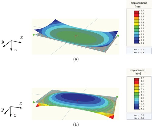
Negative eigencurvatures refer to scenarios in which the top of the plate is warmer than its bottom. The plate exhibits convex curling. Its central region lifts off from the Winkler foundation, while the corner and edge regions are pressed downwards into it, see Figure 10(b). This results in tensile curling stresses at the bottom of the plate, in the central region.

The modulus of subgrade reaction is denoted as $k_s$. A sensitivity analysis is performed, accounting for typical values of $k_s$ (Murthy 2011; Martin et al. 2016):

• $k_s=50\mathrm{MPa}/\mathrm{m}$ is representative for clays and sand,

• $k_s=100\mathrm{MPa}/\mathrm{m}$ for well-compacted sand and gravel,

• $k_s=200\mathrm{MPa}/\mathrm{m}$ for an agglomeration of crushed stone, and

• $k_s=300\mathrm{MPa}/\mathrm{m}$ for well-compacted crushed stone.

As for every nonlinear FE simulation, one specific value of the modulus of subgrade reaction and one specific value of the eigencurvature are prescribed. Once the nonlinear contact problem is solved, the software provides numerical values of the bending and twisting moments per length ($m_{xx}$, $m_{yy}$, and $m_{xy}$) at every node of the FE mesh. These output values enable the quantification of the largest principal tensile stress, see Table 4 and the markers in Figure 11, as discussed next.

Figure 11. Results from nonlinear FE analyses: largest principal tensile curling stress as a function of the eigencurvature ${\kappa }^e$ and the modulus of subgrade reaction; the markers label numerical results (see Table 4 for numerical values), the lines are splines reproducing the simulation results and interpolating between them.

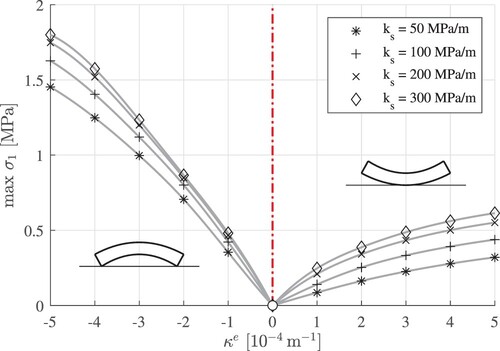
Table 4. Results from nonlinear FE analyses: largest principal tensile curling stress as a function of the eigencurvature ${\kappa }^e$ and the modulus of subgrade reaction $k_s$.

	$k_s=50$	$k_s=100$	$k_s=200$	$k_s=300$
	$\mathrm{MPa}/\mathrm{m}$	$\mathrm{MPa}/\mathrm{m}$	$\mathrm{MPa}/\mathrm{m}$	$\mathrm{MPa}/\mathrm{m}$
${\kappa }^e=-5\times {10}^{-4}/\mathrm{m}$	$1.453\mathrm{MPa}$	$1.627\mathrm{MPa}$	$1.748\mathrm{MPa}$	$1.800\mathrm{MPa}$
${\kappa }^e=-4\times {10}^{-4}/\mathrm{m}$	$1.248\mathrm{MPa}$	$1.404\mathrm{MPa}$	$1.520\mathrm{MPa}$	$1.574\mathrm{MPa}$
${\kappa }^e=-3\times {10}^{-4}/\mathrm{m}$	$0.997\mathrm{MPa}$	$1.171\mathrm{MPa}$	$1.200\mathrm{MPa}$	$1.233\mathrm{MPa}$
${\kappa }^e=-2\times {10}^{-4}/\mathrm{m}$	$0.706\mathrm{MPa}$	$0.801\mathrm{MPa}$	$0.849\mathrm{MPa}$	$0.866\mathrm{MPa}$
${\kappa }^e=-1\times {10}^{-4}/\mathrm{m}$	$0.354\mathrm{MPa}$	$0.422\mathrm{MPa}$	$0.467\mathrm{MPa}$	$0.481\mathrm{MPa}$
${\kappa }^e=+1\times {10}^{-4}/\mathrm{m}$	$0.086\mathrm{MPa}$	$0.140\mathrm{MPa}$	$0.210\mathrm{MPa}$	$0.247\mathrm{MPa}$
${\kappa }^e=+2\times {10}^{-4}/\mathrm{m}$	$0.163\mathrm{MPa}$	$0.253\mathrm{MPa}$	$0.341\mathrm{MPa}$	$0.387\mathrm{MPa}$
${\kappa }^e=+3\times {10}^{-4}/\mathrm{m}$	$0.226\mathrm{MPa}$	$0.333\mathrm{MPa}$	$0.433\mathrm{MPa}$	$0.487\mathrm{MPa}$
${\kappa }^e=+4\times {10}^{-4}/\mathrm{m}$	$0.278\mathrm{MPa}$	$0.392\mathrm{MPa}$	$0.501\mathrm{MPa}$	$0.561\mathrm{MPa}$
${\kappa }^e=+5\times {10}^{-4}/\mathrm{m}$	$0.320\mathrm{MPa}$	$0.438\mathrm{MPa}$	$0.551\mathrm{MPa}$	$0.614\mathrm{MPa}$

The largest principal tensile stress is not necessarily aligned with the x or the y-axis. Therefore, it must be determined based on extreme values of the principal bending moments per length: (22) $m_{1,2}=\frac{m_{xx}+m_{yy}}{2}\pm \sqrt{{\left(\frac{m_{xx}-m_{yy}}{2}\right)}^2+m_{xy}^2}.$(22) Positive eigencurvatures (concave curling) result in tensile stresses at the top of the plate, where $z=-h/2$. The largest principal tensile stress is obtained as (23) $max{\sigma }_1=\frac{min{m}_{1,2}}{h^3/12}\times (-\frac{h}{2})=-\frac{6min{m}_{1,2}}{h^2}.$(23) Negative eigencurvatures (convex curling) result in tensile stresses at the bottom of the plate, where $z=+h/2$. The largest principal tensile stress is obtained as (24) $max{\sigma }_1=\frac{max{m}_{1,2}}{h^3/12}\times (+\frac{h}{2})=+\frac{6max{m}_{1,2}}{h^2}.$(24) Notably, the position at which the largest principal tensile normal stress occurs, and the direction in which it is acting, change with changing values of the eigencurvature and the modulus of subgrade reaction.

Splines are used to interpolate between the computed values of the largest principal tensile stresses, see the lines in Figure 11. This allows for quantifying maximum tensile curling stresses for arbitrary values of ${\kappa }^e$ in the interval [$-5\times {10}^{-4}/\mathrm{m}$; $+5\times {10}^{-4}/\mathrm{m}$] and the four investigated values of the modulus of subgrade reaction.

3.3. Curling stresses of the monitored concrete slab

Maximum values of the tensile curling stresses, during the entire monitoring period, at the top and the bottom of the slab are quantified based on Figure 11 and extreme values of the eigencurvature. The latter are computed according to the series solution given in Table 3. The largest positive eigencurvature of the entire monitoring period, $max{\kappa }^e=+2.6\times {10}^{-4}/\mathrm{m}$, is obtained at 6:27 on 2 Oct. Corresponding tensile stress maxima refer to the top of the slab and range from $0.20\mathrm{MPa}$, obtained with $k_s=50\mathrm{MPa}/\mathrm{m}$, to $0.45\mathrm{MPa}$, obtained with $k_s=300\mathrm{MPa}/\mathrm{m}$, see Table 5. The largest negative eigencurvature of the entire monitoring period, $min{\kappa }^e=-4.8\times {10}^{-4}/\mathrm{m}$, is obtained at 15:12 on 2 Oct. Corresponding tensile stress maxima refer to the bottom of the slab and range from $1.42\mathrm{MPa}$, obtained with $k_s=50\mathrm{MPa}/\mathrm{m}$, to $1.77\mathrm{MPa}$, obtained with $k_s=300\mathrm{MPa}/\mathrm{m}$, see Table 5. These results confirm, in a quantitative fashion, that thermal curling stresses increase with an increasing modulus of subgrade reaction (Ceylan et al. 2016).

Table 5. Numerical results of maximum tensile curling stresses at the top and the bottom of the slab prescribing the largest and smallest eigencurvature of the entire monitoring period and different moduli of subgrade reaction.

$k_s$	$max{\sigma }_T({\kappa }^e)$[MPa]	$max{\sigma }_T({\kappa }^e)$[MPa]
$[\mathrm{MPa}/\mathrm{m}]$	top of slab	bottom of slab
50	0.20	1.42
100	0.31	1.60
200	0.40	1.72
300	0.45	1.77

The spatial distributions of curling stresses through the thickness of the slab are exemplarily discussed at six specific time instants of 2 Oct., see Figure 13. Thereby, $k_s$ is set equal to $100\mathrm{MPa}/\mathrm{m}$. The curling stresses are linearly distributed through the thickness of the slab. At 12:00, 15:00, and 18:00, the temperature at the top was significantly larger than at the bottom (Figure 6). This resulted in tensile stresses at the bottom of the slab, see the orange, red, and green graphs in Figure 12. In the early morning and during the nighttime, the temperature at the top was smaller than at the bottom Figure 6. This resulted in tensile stresses at the top of the slab, see the blue, magenta, and black graphs in Figure 12.

Figure 12. Exemplary results of thermo-elastic analysis: curling stress distributions through the thickness of the slab, evaluated at six time instants of 2 Oct., computed with $k_s=100\mathrm{MPa}/\mathrm{m}$.

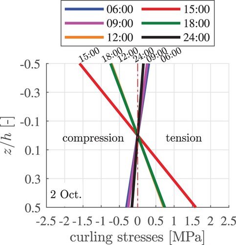
Figure 13. Exemplary results of thermo-elastic analysis: evolution of curling stresses at the top and the bottom of the slab on 2 Oct., computed with different moduli of subgrade reaction: the red markers label the maximum tensile curling stresses at the top and the bottom of the slab, in the corner regions and the central region, respectively.

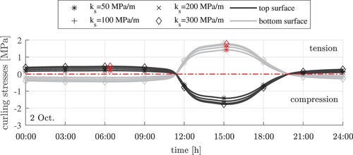
The temporal evolution of curling stresses at the top and the bottom of the slab are exemplarily discussed for 2 Oct., see Figure 13. In the morning and in the later evening, tensile curling stresses of less than 0.5 MPa are activated at the top of the slab, in its corner regions. The largest tensile stress is reached shortly after 06:00, see the red markers referring to the dark-grey graphs in Figure 13. During the afternoon, tensile curling stresses of up to more than 1.5 MPa are activated at the bottom of the slab, in its central region. The largest tensile stress is reached shortly after 15:00, see the red markers referring to the light-grey graphs in Figure 13.

3.4. Thermal eigenstresses of the monitored concrete slab

Thermal eigenstresses are independent of the modulus of subgrade reaction. They are functions of the vertical z-coordinate, and constant with respect to the in-plane x- and y-coordinates. In other words, thermal eigenstresses are constant in a specific depth, for any arbitrary location $|x|\le l_x/2$ and $|y|\le l_y/2$, rather than being restricted either to the centre or corner regions.

Maximum values of the tensile eigenstresses, during the entire monitoring period, amount to 0.64 MPa at the top of the slab, to 0.43 MPa at its midplane, and to 0.33 MPa at its bottom. Comparing these values with those listed in Table 5 underlines that the largest tensile eigenstresses reach a similar magnitude as the largest tensile curling stresses.

The spatial distributions of thermal eigenstresses through the thickness of the slab are exemplarily discussed at six specific time instants of 2 Oct., see Figure 14. Heating of the slab in the morning and during the early afternoon resulted in compressive eigenstresses in the top and bottom regions, while tensile stresses were activated around its midplane, see the orange and red graphs in Figure 14. Cooling of the slab during the later afternoon and during the nighttime resulted in tensile stresses in its top and bottom regions, while compressive stresses were activated around its midplane, see the black, blue, and green graphs in Figure 14.

Figure 14. Exemplary results of thermo-elastic analysis: thermal eigenstress distributions through the thickness of the slab, evaluated at six time instants of 2 Oct.

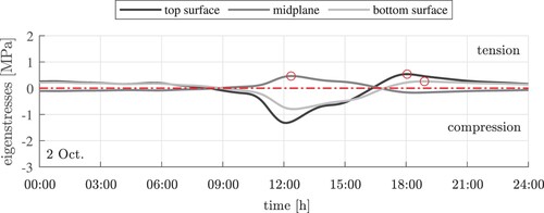
The temporal evolution of thermal eigenstresses at the top, the midplane, and the bottom of the slab are exemplarily discussed for 2 Oct., see Figure 15. At the top and the bottom of the slab, the largest tensile eigenstresses are reached in the early evening, see the red circles referring to the dark-grey and the light-grey graphs in Figure 15. At the midplane of the slab, the largest tensile eigenstress is reached shortly after 12:00, see the red marker referring to the medium-grey graph in Figure 15.

Figure 15. Exemplary results of thermo-elastic analysis: thermal eigenstresses at the top, the midplane, and the bottom of the slab on 2 Oct.: the red markers label the maximum tensile eigenstresses.

4. Significance of eigenstresses and curling stresses for total tensile thermal stresses

4.1. Total thermal stresses on 2 Oct.

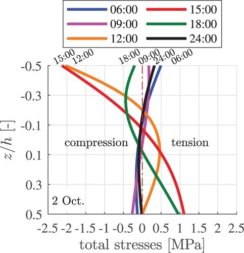
The total thermal stresses are equal to the sum of the curling stresses of Subsection 3.3 and the eigenstresses of Subsection 3.4. The spatial distributions of the total thermal stresses through the thickness of the slab are exemplarily discussed at six specific time instants of 2 Oct., see Figure 16. Thereby, $k_s$ is set equal to $100\mathrm{MPa}/\mathrm{m}$. The stress profiles are nonlinear. This confirms that thermal eigenstresses contribute considerably to the total thermal stresses, see also (Choubane and Tia 1992). The bottom of the slab experiences, in the afternoon, the overall largest total tensile stresses. At the midplane, the locally largest tensile total stresses occur around noon. At the top of the slab, the locally largest tensile total stresses occur during nighttime.

Figure 16. Exemplary results of thermo-elastic analysis: evolution of total thermal stress distributions through the thickness of the slab, evaluated at six-time instants of 2 Oct., computed with $k_s=100\mathrm{MPa}/\mathrm{m}$.

The temporal evolution of the total thermal stresses at the top and the bottom of the slab are exemplarily discussed for 2 Oct., see Figure 17. Notably, the largest tensile total stresses are smaller than the sum of the largest tensile curling stress and the largest tensile eigenstress. This will be explained in more detail in the following two paragraphs.

Figure 17. Exemplary results of thermo-elastic analysis: total thermal stresses at the top, the midplane, and the bottom of the slab on 2 Oct., computed with different moduli of subgrade reaction: the red markers label the maximum tensile curling stresses at the three different locations.

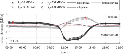
At the top of the slab, both the curling stresses and the thermal eigenstresses are tensile during nighttime, see Figures 13 and 15. Thus, the two stress contributions amplify each other, see Figures 13, 15, and 17. Still, the largest total tensile stress is smaller than the sum of the largest tensile curling stress and the largest tensile eigenstress, because the latter two maxima occur at different instants of time. The largest tensile curling stress occurred around 06:00 Figure 13, the largest tensile eigenstress around 18:00 Figure 15, and the largest total tensile stress around 01:00 Figure 17.

At the bottom of the slab, the largest tensile curling stress occurred around 15:00, see Figure 13. At that time, however, the thermal eigenstresses are compressive, see Figure 15. Thus, the two contributions counteract each other. Vice versa, the maximum tensile thermal eigenstress occurred around 19:00, see Figure 15. At that time, the tensile curling stresses are already significantly smaller compared to their preceding maximum value, see Figure 13. This explains why the maximum total tensile stress occurred in between, namely, shortly before 17:00, see Figure 17. At that time the curling stress is still quite large, see Figure 13, and the thermal eigenstress is close to its zero-crossing, see Figure 15.

4.2. Statistical analysis of daily maxima of tensile thermal stresses

Herein, the significance of eigenstresses for total thermal stresses is quantified for the top and the bottom of the slab. To this end, daily maxima of tensile curling stresses are computed, as illustrated for 2 Oct. in Figure 13. This is done for every day of the monitoring period, except for the first day, because reliable temperature fields could only be computed for the second half of that day. The daily curling stress maxima are quantified for all four values of the modulus of subgrade reaction, see columns 2, 3, 4, and 5 of Tables 6 and 7. Similarly, daily maxima of total thermal stresses are determined, as illustrated for 2 Oct. in Figure 17. These daily total stress maxima are also quantified for all four values of the modulus of subgrade reaction, see columns 6, 7, 8, and 9 of Tables 6 and 7. The daily stress maxima increase with increasing modulus of subgrade reaction.

Table 6. Daily tensile stress maxima at the top of the slab: curling stresses and total thermal stresses, evaluated for four different values of the modulus of subgrade reaction.

	daily tensile curling stress maximum [MPa]				daily tensile total stress maximum [MPa]
$k_s$[MPa/m]	50	100	200	300	50	100	200	300
24 Sept.	0.16	0.25	0.34	0.38	0.25	0.34	0.43	0.48
25 Sept.	0.12	0.19	0.27	0.31	0.27	0.33	0.41	0.45
26 Sept.	0.09	0.15	0.22	0.26	0.26	0.31	0.37	0.41
27 Sept.	0.12	0.20	0.28	0.32	0.35	0.35	0.43	0.48
28 Sept.	0.14	0.23	0.31	0.36	0.48	0.51	0.57	0.61
29 Sept.	0.18	0.27	0.36	0.41	0.38	0.47	0.55	0.60
30 Sept.	0.15	0.23	0.31	0.36	0.33	0.39	0.47	0.51
1 Oct.	0.19	0.28	0.37	0.42	0.47	0.55	0.63	0.68
2 Oct.	0.20	0.31	0.40	0.45	0.43	0.53	0.62	0.67
3 Oct.	0.13	0.20	0.29	0.33	0.33	0.38	0.45	0.49
4 Oct.	0.16	0.25	0.34	0.38	0.37	0.44	0.53	0.57
5 Oct.	0.13	0.20	0.28	0.32	0.41	0.46	0.53	0.57
6 Oct.	0.16	0.24	0.33	0.37	0.32	0.42	0.50	0.55
7 Oct.	0.05	0.09	0.14	0.17	0.14	0.17	0.22	0.25
8 Oct.	0.07	0.12	0.19	0.22	0.14	0.19	0.25	0.29
9 Oct.	0.07	0.12	0.18	0.21	0.29	0.29	0.29	0.30
10 Oct.	0.13	0.21	0.29	0.34	0.31	0.37	0.44	0.48
11 Oct.	0.17	0.26	0.35	0.40	0.36	0.44	0.53	0.57
12 Oct.	0.20	0.30	0.40	0.45	0.53	0.59	0.67	0.72
13 Oct.	0.20	0.30	0.40	0.45	0.37	0.47	0.57	0.62
14 Oct.	0.06	0.10	0.15	0.18	0.12	0.15	0.20	0.22
15 Oct.	0.06	0.10	0.15	0.18	0.08	0.11	0.17	0.20
mean values	0.13	0.21	0.29	0.33	0.32	0.38	0.45	0.49

Table 7. Daily tensile stress maxima at the bottom of the slab: curling stresses and total thermal stresses, evaluated for four different values of the modulus of subgrade reaction; empty cells refer to days, during which thermo-elastic analysis delivered only compressive stresses at the bottom of the slab.

	daily tensile curling stress maximum [MPa]				daily tensile total stress maximum[MPa]
$k_s$[MPa/m]	50	100	200	300	50	100	200	300
24 Sept.	0.14	0.18	0.21	0.22	0.09	0.12	0.14	0.15
25 Sept.
26 Sept.	0.61	0.70	0.74	0.76	0.44	0.53	0.57	0.59
27 Sept.	0.88	0.99	1.05	1.08	0.71	0.81	0.86	0.88
28 Sept.	1.24	1.39	1.50	1.56	0.98	1.12	1.22	1.27
29 Sept.	0.95	1.06	1.13	1.16	0.76	0.86	0.91	0.93
30 Sept.	0.86	0.97	1.03	1.06	0.64	0.74	0.79	0.81
1 Oct.	1.31	1.48	1.60	1.66	1.03	1.17	1.27	1.31
2 Oct.	1.42	1.60	1.72	1.77	1.14	1.29	1.40	1.46
3 Oct.	1.25	1.41	1.52	1.58	1.03	1.17	1.26	1.30
4 Oct.	1.04	1.17	1.25	1.29	0.81	0.92	0.98	1.01
5 Oct.	1.17	1.31	1.42	1.47	0.91	1.05	1.15	1.19
6 Oct.	0.95	1.07	1.14	1.17	0.73	0.84	0.90	0.92
7 Oct.
8 Oct.
9 Oct.	0.55	0.63	0.68	0.69	0.44	0.52	0.57	0.58
10 Oct.	0.09	0.11	0.13	0.14	0.07	0.05	0.07	0.07
11 Oct.
12 Oct.	0.87	0.98	1.04	1.06	0.61	0.71	0.76	0.77
13 Oct.
14 Oct.
15 Oct.	0.21	0.26	0.30	0.31	0.14	0.19	0.23	0.24
mean values	0.85	0.96	1.03	1.06	0.66	0.75	0.82	0.84

Disregarding thermal eigenstresses leads to a significant underestimation of the largest tensile total thermal stress at the top of the slab. The level of underestimation increases with decreasing modulus of subgrade reaction. Averaged over 22 days, see Table 6, it amounts to 33% for the stiffest Winkler foundation analysed: $k_s=300\mathrm{MPa}/\mathrm{m}$. This value increases to 59%, when decreasing the stiffness of the Winkler foundation to the lowest value analysed: $k_s=50\mathrm{MPa}/\mathrm{m}$, see Table 8. Vice versa, disregarding thermal eigenstresses leads to a significant overestimation of the largest tensile total thermal stress at the bottom of the slab. The level of overestimation increases with decreasing modulus of subgrade reaction. Averaged over 16 days during which tensile stresses occurred at the bottom of the slab, see Table 7, it amounts to 26% for $k_s=300\mathrm{MPa}/\mathrm{m}$ and increases to 29%, for $k_s=50\mathrm{MPa}/\mathrm{m}$, see Table 8.

Table 8. Average daily tensile stress maxima at the top and the bottom of the slab: curling stresses, total stresses, and level of over/underestimation; time period: 24 Sept. to 15 Oct.

	average daily tensile stress maxima				average daily tensile stress maxima
	at the top of the slab				at the bottom of the slab
$k_s$ [MPa/m]	50	100	200	300	50	100	200	300
total thermal stresses [MPa]	0.32	0.38	0.45	0.49	0.66	0.75	0.82	0.84
curling stresses [MPa]	0.13	0.21	0.29	0.33	0.85	0.96	1.03	1.06
misestimations [–]	$-59\text{\%}$	$-45\text{\%}$	$-36\text{\%}$	$-33\text{\%}$	$+29\text{\%}$	$+28\text{\%}$	$+26\text{\%}$	$+26\text{\%}$

5. Conclusions

From the presented analysis, the following conclusions are drawn:

• Prescribing surface temperature steps obtained from temporal interpolation and spatial extrapolation of temperatures measured inside a concrete pavement, as boundary conditions for the simulation of transient heat conduction through the slab, allows for the quasi-continuous computation of the temporal evolution of the temperature field, based on a fast-converging series solution.

• Such series solutions were also derived for quantifying the eigencurvatures of the plate (= first moment of the eigenstrain distribution) and the eigendistortions of the generators of the plate (= nonlinear part of the eigenstrain distribution).

• Curling stresses of single slabs with free edges, resulting from the eigencurvatures, can be computed as a function of the modulus of subgrade reaction, based on nonlinear finite element analyses accounting for possible partial lift-off of the plate from its Winkler foundation.

• Self-equilibrated thermal eigenstresses are directly proportional to the eigendistortions, because the generators of the plate remain virtually straight (= Kirchhoff-Love hypothesis of the linear theory for slender plates).

The presented mode of analysis provides quasi-continuous and quantitative insights into the following trends:

• Extreme values of daily thermal stresses typically occur in the early morning and in the early afternoon.

• In the early morning, the top of the slab is usually cooler than its bottom. Concave curling goes along with tensile stresses at the top and compressive stresses at the bottom. The self-equilibrated eigenstresses are tensile at the bottom and the top, and compressive around the midplane of the slab.

• In the early afternoon, the top of the slab is usually warmer than its bottom. Convex curling goes along with compressive stresses at the top and tensile stresses at the bottom. The self-equilibrated eigenstresses are compressive at the bottom and the top, and tensile around the midplane of the slab.

• Both in the early morning and in the early afternoon, the two contributions to the total thermal stresses amplify each other at the top of the slab and diminish each other at the bottom.

As regards daily maximum values of tensile thermal stresses, representing an important input for the design of concrete pavements, the following conclusions are drawn:

• Within the analysed 22 days in autumn, the average daily maximum values of the total tensile thermal stresses (= curling stresses + eigenstresses) range from 0.32 to $0.49\mathrm{MPa}$ at the top of the slab, and from 0.66 to $0.84\mathrm{MPa}$ at the bottom, for moduli of subgrade reaction ranging from 50 to $300\mathrm{MPa}/\mathrm{m}$.

• Focusing on curling stresses only, the daily maximum values of tensile stresses range from 0.13 to $0.33\mathrm{MPa}$ at the top of the slab, and from 0.85 to $1.06\mathrm{MPa}$ at the bottom, again for moduli of subgrade reaction ranging from 50 to $300\mathrm{MPa}/\mathrm{m}$.

• These results underline that disregarding thermal eigenstresses results in (i) an underestimation of the daily maximum values of tensile stresses at the top of the slab between 33 and 59 % (= quantification of stresses on the unsafe side) and (ii) an overestimation at the bottom of the slab between 26 and 29 % (= quantification of stresses on the uneconomic side). The level of misestimation increases with decreasing modulus of subgrade reaction.

• The daily maximum value of the total tensile thermal stresses is smaller than the sum of the daily maximum values of the tensile curling stresses and the tensile eigenstresses, because the latter two maxima occur at different instants of time.

Finally, it is noted that these findings may vary with slab-thickness, climate, and season.

Acknowledgments

The authors acknowlege TU Wien Bibliothek for financial support through its Open Access Funding Programme. The help of Kristina Bayraktarova (TU Wien) concerning the temperature measurements is gratefully acknowledged.

Disclosure statement

The authors report that there are no competing interests to declare.

Additional information

Funding

Financial support was provided for the temperature measurements by the Austrian Research Promotion Agency (FFG), the Austrian Ministry for Transport and Technology (bmvit), ÖBB-Infrastruktur AG (Vienna, Austria), and ASFINAG Bau Management GmbH (Vienna, Austria), VIF-2013 project ‘Optimierte Bemessung starrer Aufbauten von Straßen (OBESTAS)’ [grant number 845707]. The work of Dr Hui Wang is sponsored by Shanghai Pujiang Program [grant number 20PJ1406100].

Notes

1 Notably, the value of the modulus of elasticity of concrete is sensitive to the type of rock from which the aggregates are made, see e.g. (Ausweger et al. 2019).

Appendices

Appendix 1.

Decomposition of thermal eigenstrains

Rules for the decomposition of thermal eigenstrains follow from the Kirchhoff-Love hypothesis, stating that generators of the plate remain straight also in the deformed configuration, see also Figure A1: (A1) $u=u_m-\frac{\mathrm{\partial }{w}_m}{\mathrm{\partial }x}z,$(A1) (A2) $v=v_m-\frac{\mathrm{\partial }{w}_m}{\mathrm{\partial }y}z,$(A2) where u and v denote the displacement components in x and y-direction along the generators of the plate, $u_m$ and $v_m$ for the corresponding displacement of the midplane (hence the subscript ‘m’), and $w_m$ for the deflection. The ‘total’ normal strain components ${\epsilon }_{xx}$ and ${\epsilon }_{yy}$ of the linearised strain tensor are defined as ${\epsilon }_{xx}=\mathrm{\partial }u/\mathrm{\partial }x$ and ${\epsilon }_{yy}=\mathrm{\partial }v/\mathrm{\partial }y$. Inserting u and v according to Equations (A1(A1) $u=u_m-\frac{\mathrm{\partial }{w}_m}{\mathrm{\partial }x}z,$(A1) ) and (A2(A2) $v=v_m-\frac{\mathrm{\partial }{w}_m}{\mathrm{\partial }y}z,$(A2) ) yields (A3) ${\epsilon }_{xx}={\epsilon }_{m,x}+{\kappa }_{m,x}z,$(A3) (A4) ${\epsilon }_{yy}={\epsilon }_{m,y}+{\kappa }_{m,y}z,$(A4) where ${\epsilon }_{m,x}=\mathrm{\partial }{u}_m/\mathrm{\partial }x$ and ${\epsilon }_{m,y}=\mathrm{\partial }{v}_m/\mathrm{\partial }y$ denote the stretches of the midplane and ${\kappa }_{m,x}=-{\mathrm{\partial }}^2{w}_m/\mathrm{\partial }{x}^2$ and ${\kappa }_{m,y}=-{\mathrm{\partial }}^2{w}_m/\mathrm{\partial }{y}^2$ the curvatures of the midplane.

Figure A1. Kinematic description of the deformed configuration of a thin plate based in the Kirchhoff-Love hypothesis; after Figure  8.13 in Mang and Hofstetter (2013).

The normal stress components ${\sigma }_{xx}$ and ${\sigma }_{yy}$ of Cauchy's stress tensor read, in linear thermoelasticity, as ${\sigma }_{xx}=E[{\epsilon }_{xx}-{\epsilon }_{xx}^e+\nu ({\epsilon }_{yy}-{\epsilon }_{yy}^e)]/(1-{\nu }^2)$ and ${\sigma }_{yy}=E[{\epsilon }_{yy}-{\epsilon }_{yy}^e+\nu ({\epsilon }_{xx}-{\epsilon }_{xx}^e)]/(1-{\nu }^2)$. Inserting Equations (15(15) ${\epsilon }_{xx}^e(z,t)={\epsilon }_{yy}^e(z,t)={\epsilon }_{zz}^e(z,t)={\alpha }_T\mathrm{\Delta }T(z,t),$(15) ), (A3(A3) ${\epsilon }_{xx}={\epsilon }_{m,x}+{\kappa }_{m,x}z,$(A3) ) and (A4(A4) ${\epsilon }_{yy}={\epsilon }_{m,y}+{\kappa }_{m,y}z,$(A4) ) yields

(A5) ${\sigma }_{xx}=\frac{E}{1-{\nu }^2}[{\epsilon }_{m,x}+{\kappa }_{m,x}z-{\alpha }_T\mathrm{\Delta }T+\nu ({\epsilon }_{m,y}+{\kappa }_{m,y}z-{\alpha }_T\mathrm{\Delta }T)],$(A5) (A6) ${\sigma }_{yy}=\frac{E}{1-{\nu }^2}[{\epsilon }_{m,y}+{\kappa }_{m,y}z-{\alpha }_T\mathrm{\Delta }T+\nu ({\epsilon }_{m,x}+{\kappa }_{m,x}z-{\alpha }_T\mathrm{\Delta }T)].$(A6) Insertion of Equations (A5(A5) ${\sigma }_{xx}=\frac{E}{1-{\nu }^2}[{\epsilon }_{m,x}+{\kappa }_{m,x}z-{\alpha }_T\mathrm{\Delta }T+\nu ({\epsilon }_{m,y}+{\kappa }_{m,y}z-{\alpha }_T\mathrm{\Delta }T)],$(A5) ) and (A6(A6) ${\sigma }_{yy}=\frac{E}{1-{\nu }^2}[{\epsilon }_{m,y}+{\kappa }_{m,y}z-{\alpha }_T\mathrm{\Delta }T+\nu ({\epsilon }_{m,x}+{\kappa }_{m,x}z-{\alpha }_T\mathrm{\Delta }T)].$(A6) ) into the definition of the normal forces per length, $n_{xx}={\int }_{-\frac{h}{2}}^{+\frac{h}{2}}{\sigma }_{xx}\mathrm{d}z$ and $n_{yy}={\int }_{-\frac{h}{2}}^{+\frac{h}{2}}{\sigma }_{yy}\mathrm{d}z$, yields both the constitutive laws (A7) $n_{xx}=\frac{Eh}{1-{\nu }^2}[{\epsilon }_{m,x}-{\epsilon }^e+\nu ({\epsilon }_{m,y}-{\epsilon }^e)],$(A7) (A8) $n_{yy}=\frac{Eh}{1-{\nu }^2}[{\epsilon }_{m,y}-{\epsilon }^e+\nu ({\epsilon }_{m,x}-{\epsilon }^e)],$(A8) and the definition of the eigenstretch of the midplane of the plate, see Equation (17(17) ${\epsilon }^e(t)=\frac{1}{h}\underset{-\frac{h}{2}}{\overset{+\frac{h}{2}}{\int }}{\alpha }_T\mathrm{\Delta }T(z,t)\mathrm{d}z,$(17) ). By analogy, insertion of Equations (A5(A5) ${\sigma }_{xx}=\frac{E}{1-{\nu }^2}[{\epsilon }_{m,x}+{\kappa }_{m,x}z-{\alpha }_T\mathrm{\Delta }T+\nu ({\epsilon }_{m,y}+{\kappa }_{m,y}z-{\alpha }_T\mathrm{\Delta }T)],$(A5) ) and (A6(A6) ${\sigma }_{yy}=\frac{E}{1-{\nu }^2}[{\epsilon }_{m,y}+{\kappa }_{m,y}z-{\alpha }_T\mathrm{\Delta }T+\nu ({\epsilon }_{m,x}+{\kappa }_{m,x}z-{\alpha }_T\mathrm{\Delta }T)].$(A6) ) into the definition of the bending moments per length, $m_{xx}={\int }_{-\frac{h}{2}}^{+\frac{h}{2}}{\sigma }_{xx}z\mathrm{d}z$ and $m_{yy}={\int }_{-\frac{h}{2}}^{+\frac{h}{2}}{\sigma }_{yy}z\mathrm{d}z$, yields both the constitutive laws (A9) $m_{xx}=\frac{E{h}^3}{12(1-{\nu }^2)}[{\kappa }_{m,x}-{\kappa }^e+\nu ({\kappa }_{m,y}-{\kappa }^e)],$(A9) (A10) $m_{yy}=\frac{E{h}^3}{12(1-{\nu }^2)}[{\kappa }_{m,y}-{\kappa }^e+\nu ({\kappa }_{m,x}-{\kappa }^e)],$(A10) and the definition of the eigencurvature of the midplane of the plate, see Equation (18(18) ${\kappa }^e(t)=\frac{12}{h^3}\underset{-\frac{h}{2}}{\overset{+\frac{h}{2}}{\int }}{\alpha }_T\mathrm{\Delta }T(z,t)\cdot z\mathrm{d}z.$(18) ). Solving Equations (A7(A7) $n_{xx}=\frac{Eh}{1-{\nu }^2}[{\epsilon }_{m,x}-{\epsilon }^e+\nu ({\epsilon }_{m,y}-{\epsilon }^e)],$(A7) ) and (A8(A8) $n_{yy}=\frac{Eh}{1-{\nu }^2}[{\epsilon }_{m,y}-{\epsilon }^e+\nu ({\epsilon }_{m,x}-{\epsilon }^e)],$(A8) ) for ${\epsilon }_{m,x}$ and ${\epsilon }_{m,y}$, as well as Equations (A9(A9) $m_{xx}=\frac{E{h}^3}{12(1-{\nu }^2)}[{\kappa }_{m,x}-{\kappa }^e+\nu ({\kappa }_{m,y}-{\kappa }^e)],$(A9) ) and (A10(A10) $m_{yy}=\frac{E{h}^3}{12(1-{\nu }^2)}[{\kappa }_{m,y}-{\kappa }^e+\nu ({\kappa }_{m,x}-{\kappa }^e)],$(A10) ) for ${\kappa }_{m,x}$ and ${\kappa }_{m,x}$, and inserting the resulting expressions into Equations (A5(A5) ${\sigma }_{xx}=\frac{E}{1-{\nu }^2}[{\epsilon }_{m,x}+{\kappa }_{m,x}z-{\alpha }_T\mathrm{\Delta }T+\nu ({\epsilon }_{m,y}+{\kappa }_{m,y}z-{\alpha }_T\mathrm{\Delta }T)],$(A5) ) and (A6(A6) ${\sigma }_{yy}=\frac{E}{1-{\nu }^2}[{\epsilon }_{m,y}+{\kappa }_{m,y}z-{\alpha }_T\mathrm{\Delta }T+\nu ({\epsilon }_{m,x}+{\kappa }_{m,x}z-{\alpha }_T\mathrm{\Delta }T)].$(A6) ), yields the following expression for the normal stresses, see Equations (A11(A11) ${\sigma }_{xx}=\frac{n_{xx}}{h}+\frac{m_{xx}}{h^3/12}z-\frac{E}{1-\nu }({\alpha }_T\mathrm{\Delta }T-{\epsilon }^e-{\kappa }^{e}z),$(A11) ) and (A12(A12) ${\sigma }_{yy}=\frac{n_{yy}}{h}+\frac{m_{yy}}{h^3/12}z-\frac{E}{1-\nu }({\alpha }_T\mathrm{\Delta }T-{\epsilon }^e-{\kappa }^{e}z).$(A12) ). (A11) ${\sigma }_{xx}=\frac{n_{xx}}{h}+\frac{m_{xx}}{h^3/12}z-\frac{E}{1-\nu }({\alpha }_T\mathrm{\Delta }T-{\epsilon }^e-{\kappa }^{e}z),$(A11) (A12) ${\sigma }_{yy}=\frac{n_{yy}}{h}+\frac{m_{yy}}{h^3/12}z-\frac{E}{1-\nu }({\alpha }_T\mathrm{\Delta }T-{\epsilon }^e-{\kappa }^{e}z).$(A12) The term in the brackets of Equations (A11(A11) ${\sigma }_{xx}=\frac{n_{xx}}{h}+\frac{m_{xx}}{h^3/12}z-\frac{E}{1-\nu }({\alpha }_T\mathrm{\Delta }T-{\epsilon }^e-{\kappa }^{e}z),$(A11) ) and (A12(A12) ${\sigma }_{yy}=\frac{n_{yy}}{h}+\frac{m_{yy}}{h^3/12}z-\frac{E}{1-\nu }({\alpha }_T\mathrm{\Delta }T-{\epsilon }^e-{\kappa }^{e}z).$(A12) ) expresses the sought rule for decomposition of the thermal eigenstrains. Subtracting from the total eigenstrains, ${\alpha }_T\mathrm{\Delta }T$ the constant part related to the eigenstretch of the plate, ${\epsilon }^e$, see Equation (17(17) ${\epsilon }^e(t)=\frac{1}{h}\underset{-\frac{h}{2}}{\overset{+\frac{h}{2}}{\int }}{\alpha }_T\mathrm{\Delta }T(z,t)\mathrm{d}z,$(17) ), and the linear part related to its eigencurvature, ${\kappa }^{e}z$, see Equation (18(18) ${\kappa }^e(t)=\frac{12}{h^3}\underset{-\frac{h}{2}}{\overset{+\frac{h}{2}}{\int }}{\alpha }_T\mathrm{\Delta }T(z,t)\cdot z\mathrm{d}z.$(18) ), yields the spatially nonlinear eigendistortions of the generators of the plate, see Equation (19(19) ${\epsilon }_{dist}^e(z,t)={\alpha }_T\mathrm{\Delta }T(z,t)-{\epsilon }^e(t)-{\kappa }^e(t)\cdot z,$(19) ).

The presented derivation underlines that the developments of Thomlinson (1940) are in agreement with the linear theory of thin plates. From the viewpoint of structural mechanics, however, it is more intuitive to decompose thermal eigenstrains into a constant, a linear, and a nonlinear part, rather than performing this decomposition for the temperature.

Appendix 2.

Temperature measurements from structural monitoring

Figure A2. Temperatures measured $5\mathrm{cm}$, $9\mathrm{cm}$, $14\mathrm{cm}$ and $19\mathrm{cm}$ underneath the top surface.

References

- Armaghani J., Larsen T., and Smith L., 1987. Temperature response of concrete pavements. Transportation Research Record, 1121, 23–33.
- Ausweger M., et al., 2019. Early-age evolution of strength, stiffness, and non-aging creep of concretes: experimental characterization and correlation analysis. Materials, 12 (2), 207.
- Barber E., 1957. Calculation of maximum pavement temperatures from weather reports. Highway Research Board Bulletin, 168, 1–8.
- Barré de Saint-Venant A.J.C., 1855. Mémoire sur la torsion des prismes [essay on twisting prisms], mémoire des savant étrangers [essays of foreign scholars]. Comptes Rendues De L'Académie Des Sciencies, 14, 233–560.
- Bayraktarova K., et al., 2021. Characterisation of the climatic temperature variations in the design of rigid pavements. International Journal of Pavement Engineering, 1–14. doi: 10.1080/10298436.2021.1887486.
- Bažant Z., et al., 2015. RILEM draft recommendation: TC-242-MDC multi-decade creep and shrinkage of concrete: material model and structural analysis. Materials and Structures, 48, 753–770.
- Bentz D.P., 2000. A computer model to predict the surface temperature and time-of-wetness of concrete pavements and bridge decks. National Institute of Standards and Technology – Technology Administration, U.S. Department of Commerce.
- Bradbury R.D., 1938. Reinforced concrete pavements. University of Wisconsin – Madison: Wire Reinforcement Institute.
- Ceylan H., et al., 2016. Impact of curling and warping on concrete pavement. Program for Sustainable Pavement Engineering and Research. Ames, IA: Institute for Transportation, Iowa State University.
- Choubane B., and Tia M., 1992. Nonlinear temperature gradient effect on maximum warping stresses in rigid pavements. Transportation Research Record, 1370, 11–19.
- Choubane B., and Tia M., 1995. Analysis and verification of thermal-gradient effects on concrete pavement. Journal of Transportation Engineering, 121 (1), 75–81.
- Díaz Flores R., et al., 2021. Multi-directional falling weight deflectometer (FWD) testing and quantification of the effective modulus of subgrade reaction for concrete roads. International Journal of Pavement Engineering, 1–19. doi: 10.1080/10298436.2021.2006651.
- Dlubal Software GmbH, 2020. RFEM – FEM structural analysis software.
- Hiller J.E., and Roesler J.R., 2010. Simplified nonlinear temperature curling analysis for jointed concrete pavements. Journal of Transportation Engineering, 136, 654–663.
- Höller R., et al., 2019. Rigorous amendment of vlasov's theory for thin elastic plates on elastic winkler foundations, based on the principle of virtual power. European Journal of Mechanics/ A Solids, 73, 449–482.
- Ioannides A.M., and Khazanovich L., 1998. Nonlinear temperature effects on multilayered concrete pavements. Journal of Transportation Engineering, 124, 128–136.
- Janssen D.J., and Snyder M.B., 2000. Temperature-moment concept for evaluating pavement temperature data. Journal of Infrastructure Systems, 6, 81–83.
- Khazanovich L., 1994. Structural analysis of multi-layered concrete pavement systems. Thesis (PhD). University of Illinois at Urbana-Champaign.
- Khazanovich L., et al., 2001. Development of rapid solutions for prediction of critical continuously reinforced concrete pavement stresses. Transportation Research Record, 1778, 64–72.
- Kuo C.M., Hall K.T., and Darter M.I., 1995. Three-dimensional finite element model for analysis of concrete pavement support. Transportation Research Record, 1505, 119–127.
- Liang S., and Wei Y., 2018. Modelling of creep effect on moisture warping and stress developments in concrete pavement slabs. International Journal of Pavement Engineering, 19 (5), 429–438.
- Louhghalam A., Petersen T., and Ulm F.J., 2018. Translating environmentally-induced eigenstresses to risk of fracture for design of durable concrete pavements. Computational modelling of concrete structures. CRC Press, 265–273.
- Mang H.A., and Hofstetter G., 2013. Festigkeitslehre. 4th ed., Springer Vieweg.
- Martin U., et al., 2016. Abschätzung der Untergrundverhältnisse am Bahnkörper anhand des Bettungsmoduls [in German]. ETR-Eisenbahntechnische Rundschau, 5, 50–57.
- MEPDG, 2008. Mechanistic-empirical pavement design guide: a manual of practice. AASHTO.
- Mohamed A.R., and Hansen W., 1997. Effect of nonlinear temperature gradient on curling stress in concrete pavements. Transportation Research Record, 1568, 65–71.
- Murthy V., 2011. Textbook of soil mechanics and foundation engineering. CBS Publisher & Distributors/Alkem Company (S).
- NCHRP, 2004. Guide for mechanistic-empirical design of new and rehabilitated pavement structures. Transportation Research Board. Washington, DC, USA, ARA, Inc., ERES Division, 505 West University Avenue, Champaign, Illinois 61820. Project 1-37A.
- Neville A.M., 1995. Properties of concrete. Vol. 4, London: Longman.
- Qin Y., 2016. Pavement surface maximum temperature increases linearly with solar absorption and reciprocal thermal inertial. International Journal of Heat and Mass Transfer, 97, 391–399.
- Sarkar A., and Norouzi R., 2020. Evaluating curling stress of continuous reinforced concrete pavement. ACI Structural Journal, 117 (1), 53–62.
- Sen S., and Khazanovich L., 2021. Reconsidering the strength of concrete pavements. International Journal of Pavement Engineering, 1–11. doi: 10.1080/10298436.2021.2020270.
- Siddique Z.Q., Hossain M., and Meggers D., 2005. Temperature and curling measurements on concrete pavement. Proceedings of the Mid-Continent Transportation Research Symposium 2005. Ames, Iowa, USA. Ames, Iowa, USA, 1–12.
- Sii H. B., et al., 2014. Development of prediction model for doweled joint concrete pavement using three-dimensional finite element analysis. Applied Mechanics and Materials, 587, 1047–1057.
- Tabatabaie A.M., and Barenberg E.J., 1978. Finite-element analysis of jointed or cracked concrete pavements. Transportation Research Record, 671, 11–19.
- Teller L., and Sutherland C., 1935. The structural design of concrete pavements; parts 1+2. Division of Tests, Bureau of Public Roads, 16 (8-9), 145–189.
- Thomlinson J., 1940. Temperature variations and consequent stresses produced by daily and seasonal temperature cycles in concrete slabs. Concrete Constructional Engineering, 36 (6), 298–307.
- Time & Date, A, 2020. Wetterrückblick für Bad Vöslau, Niederösterreich, Österreich – Oktober 2015. Available from: https://www.timeanddate.de/wetter/oesterreich/bad-voeslau/rueckblick?month=10&year=2015. [Accessed 1 March 2022].
- Wang H., et al., 2019a. Concrete pavements subjected to hail showers: A semi-analytical thermoelastic multiscale analysis. Engineering Structures, 200, 109677.
- Wang H., et al., 2019b. Multiscale thermoelastic analysis of the thermal expansion coefficient and of microscopic thermal stresses of mature concrete. Materials, 12 (17), 2689.
- Wei Y., et al., 2019. Nonlinear strain distribution in a field-instrumented concrete pavement slab in response to environmental effects. Road Materials and Pavement Design, 20 (2), 367–380.
- Wei Y., Liang S., and Gao X., 2017. Numerical evaluation of moisture warping and stress in concrete pavement slabs with different water-to-cement ratio and thickness. Journal of Engineering Mechanics, 143 (2), 04016111.
- Westergaard H., 1927. Analysis of stresses in concrete pavements due to variations of temperature. Highway Research Board Proceedings, 6, 201–215.
- Winkler E., 1867. Die Lehre von der Elastizität und Festigkeit: Mit besonderer Rücksicht auf ihre Anwendung in der Technik; für polytechnische Schulen, Bauakademien, Ingenieure, Maschinenbauer, Architekten etc. [Lessons on elasticity and strength of materials: with special consideration of their application in technology; for polytechnical schools, building academies, engineers, mechanical engineers, architects, etc]. Dominicus.
- Yu H.T., Khazanovich L., and Darter M.I., 2004. Consideration of JPCP curling and warping in the 2002 design guide. CD-ROM Proceedings of the 83rd Annual Meeting of the Transportation Research Board.
- Zhang J., et al., 2003. Model for nonlinear thermal effect on pavement warping stresses. Journal of Transportation Engineering, 129 (6), 695–702.