Experimental Measurements of Oil Films in a Dynamically Loaded Journal Bearing

Abstract

This article describes the design of a journal bearing test platform capable of high-accuracy film thickness measurements via ultrasonic transducers permanently embedded in both the bearing and rotating shaft. A bespoke hydraulic loading system with programmable valves allowed the application of dynamic loads with defined loading patterns, including the simulation of loading patterns found in real components such as automotive connecting rod bearings. Tests under a range of rotation speeds, temperatures, and loading profiles allowed the detailed analysis of film thickness response to rapidly changing loads. Unlike conventional methods, the ultrasonic technique offers a noninvasive direct measurement of the shaft–bearing interface, thus enabling the study of phenomena such as squeeze film effects. Measurements were achieved by applying a novel referencing method, referred to as the “snapshot technique”. Via this method, squeeze time was shown to reduce with increasing shaft rotation speed, applied load, and bearing temperature. Results were compared against inductive sensors and numerical techniques and good agreement was observed.

Keywords:

• Oil film thickness measurement
• ultrasound
• journal bearing
• dynamic loading
• snapshot technique
• squeeze film

Introduction

Due to their large contact area, journal bearings offer excellent protection against rapid dynamic loads compared to other bearing types such as ball bearings (1). However, journal bearings have their limits and, as they are pushed to operate under ever more demanding conditions, the mechanics of dynamic loading must be well understood.

Shock loading is an undesirable sudden spike in applied load, commonly experienced in many dynamic applications; for example, in suspension systems when a car hits a bump or marine stern tubes when the propeller crashes into a wave in stormy weather (2). This sudden increase in load reduces film thickness and can cause metal-to-metal contact if not properly controlled. However, predicting minimum film thickness is not as simple as considering a static load of the same magnitude. This is because the oil cannot enter or exit the contact instantly, no matter how hard it is squeezed. The effect is known as a “squeeze film” and the delay period is referred to as “squeeze time”. This squeeze time is related to the magnitude of the applied load, bearing geometry, and oil viscosity (3).

Squeeze films can be inherently useful because they offer a level of cushioning against extreme loads, although only for a short period of time. In many applications, it is critical to correctly predict the squeeze film effect. An underestimation will mean that an unnecessarily high viscosity oil is used, thus reducing efficiency, whereas an overestimation will lead to instability, vibrations, and wear due to shaft–bearing contact (4). How the film recovers after load removal is equally important, because the oil layer must be sufficiently thick to protect the system from the next load instance.

Automotive connecting rod bearings are a common example of bearings subjected to dynamic loading. They convert linear reciprocating motion to a transient cyclic rotation, and so understanding their behavior is particularly challenging. The magnitude of the load as well as its radial direction (5). This variation rapidly changes both minimum film thickness and attitude angle significantly. Connecting rod bearing failure can have catastrophic effects, potentially causing the connecting rod to snap (known colloquially as” throwing a rod”) and driving it through the crankcase, thereby destroying the engine. Thus, engine manufacturers have a vested interest in optimizing efficiency by minimizing film thickness, while mitigating the possibility of bearing failure.

Along with an increasing understanding of dynamic loading in traditional bearings, new bearing designs to mitigate dynamic loading effects have also been developed (6). Applications that require even more protection against shock loading can implement a squeeze film damping system between the bearing and housing. However, these are not suitable for lower cost or compact systems because the feature requires additional thickness around the bearing circumference.

Several techniques have been developed in an attempt to understand dynamically loaded bearing behavior. In 2016, Gong et al. presented an analytical solution that applies to dynamic loading operating conditions, derived using the regular perturbation method (7). The mobility method, introduced by Booker (8) in 1965, provides a numerical solution to dynamically loaded bearings. Although this method is decades old, it is still frequently used and being built upon. A good example is Park et al., who in 2020 adapted the mobility method to investigate journal bearings under dynamic loads using non-Newtonian fluids, with con-rod bearings as the intended application (9). However, the fundamental limitation with predictive methods is that they must balance complexity with the number of assumptions made. To account for effects such as temperature and deformation, all component geometries and material types need to be modelled accurately. As such, the results are only as good as the model. Often it is difficult to obtain all parameters, and these are subject to change over time due to effects such as wear (10).

Experimental techniques such as the total capacitance method (TCM) enable the measurement of bearing film thickness within real systems. As its name suggests, TCM measures the capacitance across the interface and uses the dialectic constant of the oil to infer minimum film thickness. TCM was applied to crankshaft bearings in an operating engine by Kataoka et al. in 2011 (11). However, this study concluded that TCM does not take into account deformation in the bearing or crankshaft.

Inductive sensors are also a popular technology applied to film thickness measurements. In 2002, Moreau et al. implemented inductive sensors into a con-rod bearing test platform to study dynamic loading conditions and compare measurements against a theoretical model (12). Four sensors were embedded in the bearing at different locations around its circumference. This allowed a direct measurement of film thickness at distinct points; however, accuracy was limited to ±1 μm and the presence of a surface-mounted sensor within the contact may have affected bearing operation.

Ultrasound has the potential to overcome the limitations of conventional methods, particularly because the sensors can be positioned away from the shaft–bearing interface, thus providing a direct measurement without influencing bearing operation. The application of ultrasound to the study of journal bearing behaviour began to emerge in the early 2000s. In 2008, Kasolang and Dwyer-Joyce used shaft-mounted transducers to obtain circumferential measurements under normal operating conditions via the spring amplitude technique (13). In this work, signs of cavitation in the diverging region could be clearly identified. However, due to the limited range of the amplitude technique, measured film thickness ranged only between 10 and 40 μm in their study. In 2020, Ouyang et al. extended the versatility of shaft-mounted ultrasound by applying the spring amplitude and resonant dip techniques simultaneously (14). This enabled a wider range of oil films to be measured. However, a gap in the measurable range between thin-film measurements via the amplitude method and thick-film measurements via the resonant dip method still existed.

Previous studies applying ultrasound to journal bearings have concentrated only on normal operating conditions, in which operational parameters such as rotation speed and applied load are constant. Researching more severe conditions such as dynamic loading could extend the utility of the ultrasound technique, enabling its use in a wider range of applications.

Dynamic loading bearing test platform

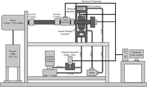
The following section details the primary mechanical components and instrumentation used in the test platform for this investigation. A photograph of the platform in operation is provided in Fig. 1, along with a schematic of the system in Fig. 2.

Figure 1. (a) Photograph of dynamic loading test rig in operation. (b) Close-up view of bearing assembly. (c) Close-up view of acquisition hardware.

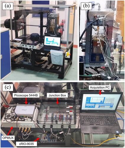
Figure 2. Schematic of bearing test platform.

Mechanical components

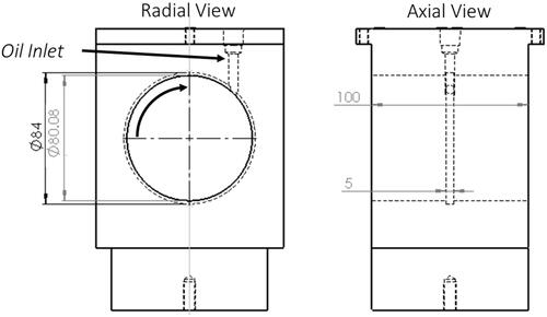
The bearing assembly consisted of an EN24T steel shaft running inside a solid aluminium bronze (C95400, ${\text{CuAl}}_{11}{\text{Fe}}_4$) bush. Dimensions of the aluminum bronze bush are provided in Fig. 3. This geometry included a single circumferential groove running around the axial center of the bearing. The inclusion of a circumferential groove is suitable for bearings subject to dynamic loads due to the wide range of attitude angles they experience. The groove allowed oil to reach the changing minimum film region more easily, reducing the chance of starvation.

Figure 3. Dimensioned schematic of the bearing used in the test platform. Curved arrow indicates the direction of shaft rotation.

The shaft was also supported by two needle roller bearings on either side of the bronze bush, along with needle thrust bearings at each end of the shaft. These thrust bearings prohibited the shaft from rubbing directly onto the sides of the housing in the event of axial movement. A section view of the housing assembly is shown in Fig. 4.

Figure 4. Annotated CAD renders of bearing test platform. (a) Dimetric projection of full assembly. (b) Section view of bearing housing. Cabling and hydraulic hose circuit omitted for clarity.

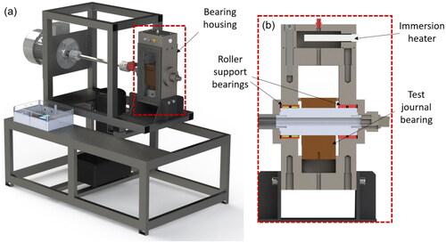
The bearing was lubricated via a continuous oil circulation system, pumped at a pressure of 2 bar into the bearing contact via the oil inlet annotated in Fig. 3. Lubricant temperature was controlled via an immersion heater located in a manifold on top of the bearing housing, shown in Fig. 4.

A primary function of the bearing test platform presented was its dynamic loading capability. This was achieved via a hydraulic power pack that applied pressure to the bottom face of the bearing bush, pushing it upwards like a piston. The applied pressure could then be varied by controlling an electro-proportional valve. Opening the valve allowed fluid to flow more freely through the circuit, relieving pressure, whereas closing the valve blocked flow, thereby increasing pressure. The magnitude of applied pressure was controlled by adjusting the voltage output to the valve via an embedded controller and voltage output module.

Pressure in the hydraulic circuit can be easily converted to applied load by multiplying by the area of the bearing bottom face (7,854 mm²). A nitrile seal fitted between the bearing and bore prevented cross-contamination between the lubrication circuit and hydraulic loading circuit; however, because some leakage may occur, the same oil was used in both circuits as a precaution.

A sample of the load cycles trialled is presented in Fig. 5. These are constant load, sine wave, and square wave loading patterns. In this case, loading patterns were synchronized to shaft rotation angle via an encoder, with the sine wave pattern repeating every 360° and the square wave every 720°. Load was only applied for one-quarter of the square wave cycle to simulate real four-stroke engine loading more closely. Examples with a shaft rotation speed of 100 and 700 rpm are presented.

Figure 5. Example load cycles from bearing test platform (constant load, sine wave and square wave) at (a) 100 rpm and (b) 700 rpm.

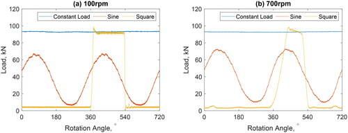
At 100 rpm both the sine and square wave loading patterns closely follow the desired input. However, at 700 rpm there is a moderate rise time for the square wave loading pattern. This is because the valve does not close instantly and also because the oil is not perfectly incompressible. Although acceptable for this work, rise time could be mitigated in the future by reducing the hose length between the power pack and journal assembly, thus reducing the volume of the working fluid, or by using a faster acting valve.

Key values for the test platform geometry and operating parameters used in this investigation are presented in Table 1. The shaft, bearing, and lubricant material properties are detailed in Table 2. Bearing dimensions and operating conditions were selected to match those found in real systems, in particular connecting rod big-end bearings (15–17). Clearance was validated during the manufacturing stage by measuring the shaft diameter using micrometers and the bush internal diameter using telescopic gauges.

Table 1. Test platform geometry and operating parameters.

Parameter	Value
Bearing radial clearance, C	50 μm ($\pm \hspace{0.17em}5\mu$m)
Bearing internal diameter, D	80 mm
Bearing length, L	100 mm
Load range, W	2–100 kN
Rotation speed, N	50–700 rpm

Table 2. Material and lubricant properties.

Material property	Value
Acoustic impedance of bearing, z2	38.1 MRayl
Acoustic impedance of shaft, z1	46 MRayl
Oil density, ρ	$888/(1+0.0007(T-20))$kgm^–3
Oil acoustic velocity, c	$(0.0039T^2-3.39T+1555.2)$ms^−1
Oil kinematic viscosity at 40${}^{°}$C	104 cP
Oil kinematic viscosity at 100${}^{°}$C	11.6 cP

Conventional instrumentation

The test platform included conventional hardware to measure torque, load, rotation speed, and temperature. Thermocouples were located within the heater manifold, annotated in Fig. 2, to measure oil inlet temperature. Thermocouples were also positioned at the edges of the bearing, touching the running face of the shaft to record bearing operating temperature. A transducer measured torque and provided a TTL (transistor–transistor logic) pulse once per degree of shaft rotation. This was used in conjunction with a Hall effect sensor that provided a TTL pulse each full revolution. Additionally, two pressures were installed; one monitored oil inlet pressure and one indirectly measured applied bearing load.

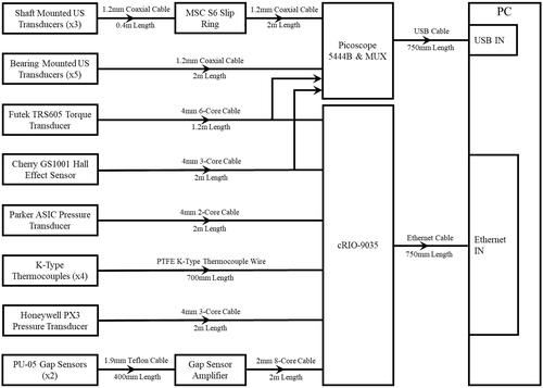
The analog measurement devices were controlled by an embedded controller linked to an acquisition PC. The embedded controller features an FPGA (field-programmable gate array), enabling the system to run efficiently with very high capture rates, up to 10 MHz. A measurement hardware flow diagram describing how each component was linked is provided in Fig. 6.

Figure 6. Measurement hardware flow diagram for bearing test platform.

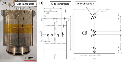
Two inductive gap sensors were mounted onto the bearing bush, allowing ultrasonic measurement to be compared against those from a conventional technique. The positions of these gap sensors are highlighted in Fig. 7.

Figure 7. (a) Photograph of bearing side view, taken during ultrasonic transducer instrumentation before wires were soldered to each element. (b) Dimensioned drawing of bearing side view and top view, detailing size and locations of bearing-mounted ultrasound transducers, along with transducer numbering notation. The position of inductive (gap) sensors is also indicated. Thermocouples are also located alongside each gap sensor.

Ultrasonic instrumentation

The bearing test platform was instrumented with ultrasonic longitudinal transducers permanently bonded on both the shaft and bearing to provide film thickness measurements. A total of 12 elements were instrumented on the bronze bush, 4 on each side and 4 on the top face. The side-mounted bearing transducer elements were soft-PZT, with a center frequency of 5 MHz (18). The top-mounted bearing transducers had a center frequency of 10 MHz (19). The transducer center frequency had to be carefully selected to provide optimum signal-to-noise ratio within the expected measurement range (20).

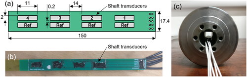
The shaft was instrumented with eight soft-PZT transducer elements, each with a center frequency of 5 MHz. The positions and dimensions of the bearing-mounted transducers and shaft-mounted transducers are shown in Figs. 7 and 8, respectively.

Figure 8. (a) Dimensioned drawing of shaft-side ultrasonic transducer array. (b) Photograph of shaft-side array taken before shaft installation; piezoceramic elements are covered with epoxy adhesive. (c) Photograph of shaft-side array embedded within the shaft bore, taken before test platform assembly.

During operation, transducer elements were excited by an electrical pulse. This pulse was then converted into an acoustic wave via the piezoelectric effect. The wave then traveled through the bearing and hit the bearing–shaft interface. At this interface some of the acoustic energy was reflected back toward the transducer, and the remaining energy was transmitted through the interface. The proportion of the energy reflected at the interface compared to the total energy is known as the “reflection coefficient”, R, and is dependent on the acoustic impedance mismatch between layers (21). In a thin three-layer system there is also a change in signal phase at the interface.

The bearing-mounted transducers operated in a pulse-echo configuration, in which the same transducers both transmitted and received the acoustic signal, whereas the shaft-mounted transducers operated in a pitch–catch configuration, in which one set of transducers generated the acoustic wave and another set received the reflected wave. The pitch transducers are denoted as “Ref” and the catch transducers are numbered 1 to 4 in Fig. 8.

In the test platform, bearing and shaft ultrasonic transducers were excited sequentially by a multiplexer. The signal response was then captured by a PC-based USB oscilloscope. Excitation pulses were triggered by the rotation of the shaft. A TTL signal was produced per single degree rotation by a shaft encoder integrated into the torque transducer. This signal fed into a digital output module, which was programmed to output eight TTL signals in quick succession (at 24 μs intervals). These eight signals were sent to the multiplexer and oscilloscope to trigger ultrasonic signal generation and capture. Multiplying one TTL signal to an eight-signal pulse train in this manner allowed the system to capture an ultrasound response on all eight channels at essentially the same shaft position.

Film thickness acquisition methodology

Active ultrasonic transducers are capable of measuring oil film thickness by pulsing a high-frequency sound wave at the lubricated interface and studying changes in the reflected wave. This reflected wave is recorded by either the same or a nearby transducer. Changes could include variations in signal amplitude, frequency phase, or time delay. The most appropriate technique is dependent on the expected film thickness range (22).

If the oil film is thin (on the order of one to tens of micrometers), the phase shift technique, developed by Reddyhoff et al. (23), is suitable. As its name suggests, this method observes the difference in phase between the incident and reflected signals at a particular frequency. The relation between phase shift and film thickness can be expressed by the following: [1] $$h=\frac{\rho c^2(\hspace{0.17em}\mathit{\text{tan}}\hspace{0.17em}{\Phi }_R)(z_1^2-z_2^2)}{\omega z_1{z}_2\pm \sqrt{{(\omega z_1{z}_2^2)}^2-{(\hspace{0.17em}\mathit{\text{tan}}\hspace{0.17em}{\Phi }_R)}^2(z_1^2-z_2^2){(\omega z_1{z}_2)}^2}},$$[1] where h is the film thickness, ρ is the lubricant density, c is the lubricant acoustic velocity, ${\Phi }_R$ is the phase shift between the reflected and incident signal, ω is the wave angular frequency, and z₁ and z₂ are the acoustic impedances of the first and second solid layers. The phase shift technique was selected as a suitable method for the side bearing-mounted transducers.

The measurement uncertainty for the phase shift technique is proportional to oil film thickness, meaning that this method is most accurate for thinner films. In theory the phase shift measurement range is infinite; however, as phase shift tends to zero, any noise in the signal begins to dominate any observed change (23). For this study, a threshold phase shift of 0.05 rad one to tens of micrometers was selected. With a resolution of 0.01 rad, this corresponds to a maximum uncertainty of ±4.3 μm at 48 μm. Thinner film measurements in this study would have a much lower uncertainty; for example, a measurement of 5 μm would have an uncertainty of ±0.07 μm. A more in-depth exploration of measurement uncertainty for the phase shift method can be found in previous literature (23, 24).

For the top-mounted bearing transducers the expected oil film thickness was greater than the phase shift measurement range. Therefore, an alternative model is required, specifically the film resonance technique. This can be expressed by the following: [2] $$f_m=\frac{cm}{2h},$$[2] where f_m is film resonance frequency and m is the resonance mode.

The primary consideration when applying the resonance method is having confidence that the determined resonance mode of the observed dip is correct. In this case it was clear that the fundamental frequency was being observed (i.e., m = 1). This was determined as the maximum oil film thickness is limited by the diametric clearance of the bearing. For the observed dip to be anything other than the fundamental frequency (i.e., m > 1), the measured film would significantly exceed the diametric clearance and so would not make logical sense.

The uncertainty in the resonance technique is driven by uncertainty in the lubricant acoustic velocity values (used in Eq. [2][2] $$f_m=\frac{cm}{2h},$$[2] ). This acoustic velocity is determined prior to testing across a temperature range between 20 and 130 °C using a calibration rig to a high accuracy ($<\pm$0.1%). Acoustic velocity decreases linearly with temperature, which is measured during operation. The measurement accuracy of the thermocouples is ±1.5 °C which results in an acoustic velocity uncertainty of 4.5 ms^–1 and therefore uncertainty in film measurements of 0.3%.

During each rotation, the shaft-mounted transducers observed a range of film thicknesses spanning across the phase shift and film resonance measurement ranges. Thus, a combination of the techniques was used to capture a more complete circumferential film thickness profile, although the minimum film region was generally of most interest in this investigation, measured via the phase shift method. The techniques used for each set of transducers are shown in Fig. 9.

Figure 9. Schematic of bearing assembly, highlighting the ultrasonic methods used for each set of transducers.

Obtaining a reference signal

Ultrasonic film thickness methods, including the phase shift technique, require a reference signal. This reference signal has a known reflection coefficient amplitude and phase, which can be compared against the measurement signal. For example, in a solid–air boundary, practically all of the signal energy is reflected ($R\approx 1$) and the reflected signal phase is reversed by π radians. This is due to the extreme acoustic impedance mismatch between solid materials and air (23).

The most common referencing technique is known as a “pretest reference”. This often involves placing the instrumented component in an oven and recording the signal response over the range of temperatures expected during operation. However, the temperature gradient will differ between the pretest reference and during normal operation. This can lead to significant uncertainties in film measurements. Also, the system would need to be disassembled and a new reference taken if any degradation of the elements occurred (24).

To maximize measurement accuracy, the shaft-mounted transducers used the “infinite film” reference technique. This involves taking a reference during operation when the transducer rotation angle is within the thick-film region of the bearing and is therefore outside of the phase shift measurement range. Thus, the interface can be modeled as a simple two-layer solid–oil boundary, with a defined reflection coefficient and phase. This was proven to be a robust technique in a previous study (24).

Because the top bearing transducers employed the film resonance technique for film thickness measurements, they did not require a reference measurement. However, the side-mounted bearing transducers remained within the phase shift measurement range at all times during operation and expected oil thickness was too thin for the film resonance technique. As a result, either a conventional pretest reference or an alternative method is required. Unfortunately, due to the sensitivity of the phase shift technique to effects such as changes in temperature gradient through the bearing material, a pretest reference was found to be inadequate. As such, an alternative technique was created.

The following new referencing method proposed will henceforth be referred to as the “snapshot” reference technique in this work, because it takes the film thickness information from other sensors at a single moment in time and uses geometry to infer the expected film thickness and then a reference phase for the transducers in question. The step-by-step process for this technique is shown in Fig. 10.

Figure 10. Flow diagram detailing the routine for applying the snapshot reference technique. The phase equation is shown in Eq. [1][1] $$h=\frac{\rho c^2(\hspace{0.17em}\mathit{\text{tan}}\hspace{0.17em}{\Phi }_R)(z_1^2-z_2^2)}{\omega z_1{z}_2\pm \sqrt{{(\omega z_1{z}_2^2)}^2-{(\hspace{0.17em}\mathit{\text{tan}}\hspace{0.17em}{\Phi }_R)}^2(z_1^2-z_2^2){(\omega z_1{z}_2)}^2}},$$[1] .

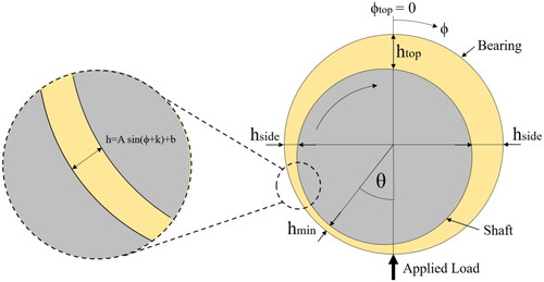
To model the system geometrically, the shaft and bearing surfaces can be treated as two concentric circles (as shown in Fig. 11). Assuming the distance between circles (i.e., film thickness) is small compared to their radii, the distance between circles around the circumference can be approximated via the following: [3] $$h=f(\varphi )=A \hspace{0.17em}\mathit{\text{sin}}(\varphi +k)+b,$$[3] where $\varphi$ is the bearing angle and A, b, and k are constants unique to a particular geometry. These constants can be calculated via the following three equations given that the minimum film thickness, attitude angle, and film thickness at the top of the bearing are known: [4] $$A=\frac{h_{\mathit{top}}-h_{\mathit{min}}}{\hspace{0.17em}\mathit{\text{sin}}\left({\varphi }_{\mathit{top}}+\frac{(2n+1)\pi }{2}-\theta \right)-\hspace{0.17em}\mathit{\text{sin}}\left(\frac{(2n+1)\pi }{2}\right)}$$[4] [5] $$b=h_{\mathit{min}}-A \hspace{0.17em}\mathit{\text{sin}}\left(\frac{(2n+1)\pi }{2}\right)$$[5] [6] $$k=\frac{(2n+1)\pi }{2}-\theta ,$$[6] where h_top is the film thickness at the top of the bearing, h_min is minimum film thickness, ${\varphi }_{\mathit{top}}$ is the angle at the top of the bearing (in this work defined as 0°), and θ is attitude angle.

Figure 11. Schematic of bearing geometry, with h_min, h_top, and θ denoting minimum film thickness, top bearing film thickness, and attitude angle, respectively.

The derivation of these constants is found via applying the following boundary conditions: [7] $$f(\theta )=h_{\mathit{min}}=\mathit{Asin}(\theta +k)+b$$[7] [8] $$f({\varphi }_{\mathit{top}})=h_{\mathit{top}}=\mathit{Asin}({\varphi }_{\mathbf{top}}+\mathbf{k})+b.$$[8]

Because the gradient at the point of minimum film thickness is zero, the derivative of Eq. [7][7] $$f(\theta )=h_{\mathit{min}}=\mathit{Asin}(\theta +k)+b$$[7] provides an additional boundary condition: [9] $$f\prime (\theta )=0=\mathit{Asin}(\theta +k)+b.$$[9]

Film thickness at the position of each side sensor can then be calculated via Eq. [3][3] $$h=f(\varphi )=A \hspace{0.17em}\mathit{\text{sin}}(\varphi +k)+b,$$[3] , in this work defined as 90° and 270${}^{°}$.

The phase equation (Eq. [1][1] $$h=\frac{\rho c^2(\hspace{0.17em}\mathit{\text{tan}}\hspace{0.17em}{\Phi }_R)(z_1^2-z_2^2)}{\omega z_1{z}_2\pm \sqrt{{(\omega z_1{z}_2^2)}^2-{(\hspace{0.17em}\mathit{\text{tan}}\hspace{0.17em}{\Phi }_R)}^2(z_1^2-z_2^2){(\omega z_1{z}_2)}^2}},$$[1] ) can be rearranged to make $\Phi$ the subject: [10] $$\Phi =\mathit{atan}\left(\frac{2z_1{z}_2^2(\omega /K)}{(z_1^2-z_2^2)+z_1^2{z}_2^2{(\omega /K)}^2}\right)$$[10] for which [11] $$K=\frac{\rho c^2}{h},$$[11] where K is the stiffness. Also note the distinction between bearing angle $\varphi$, ultrasonic wave phase angle $\phi$, and ultrasonic wave phase shift $\Phi$.

Applying side film thickness found geometrically to Eqs. [10][10] $$\Phi =\mathit{atan}\left(\frac{2z_1{z}_2^2(\omega /K)}{(z_1^2-z_2^2)+z_1^2{z}_2^2{(\omega /K)}^2}\right)$$[10] and [11][11] $$K=\frac{\rho c^2}{h},$$[11] thus allows phase shift to be calculated. Subtracting the phase measured from the side sensor from this phase shift then provides a reference phase value. This reference phase, in theory, would be equal to a phase measurement taken at a solid–air or solid–infinitely thick oil film boundary.

A more common method to calculate film thickness around the circumference is through the following relationship: [12] $$h=C(1+\epsilon \hspace{0.17em}\mathit{\text{cos}}\hspace{0.17em}(\theta )).$$[12]

However, this requires knowledge of clearance as an input. The advantage of the presented technique is that clearance is not required but only minimum film thickness, attitude angle, and film thickness measured at one other location, in this case at the top of the bearing. Clearance can change significantly during operation in journal bearing systems, particularly if the shaft and bearing materials have different thermal expansion coefficients and the system operates over a wide range of temperatures.

Results and discussion

The following covers results obtained via the bearing test platform under a range of static and dynamic loading conditions. First, measurements from shaft-mounted transducers are presented. This is followed by bearing-mounted sensor measurements that enable continuous monitoring of minimum film thickness and attitude angle. Measurements are then compared against predictions from a numerical model and measurements from bearing-mounted inductive sensors.

Shaft sensor film thickness measurements

Examples of reflected time and frequency phase domain signal responses taken from shaft sensor 2 are presented in Figs. 12a and 12b, respectively. These show a comparison between signals taken within the thin film and infinite film regions. Figure 12b highlights a phase shift across all frequencies, although this shift reduces with increasing frequency. This observation aligns with Eq. [1][1] $$h=\frac{\rho c^2(\hspace{0.17em}\mathit{\text{tan}}\hspace{0.17em}{\Phi }_R)(z_1^2-z_2^2)}{\omega z_1{z}_2\pm \sqrt{{(\omega z_1{z}_2^2)}^2-{(\hspace{0.17em}\mathit{\text{tan}}\hspace{0.17em}{\Phi }_R)}^2(z_1^2-z_2^2){(\omega z_1{z}_2)}^2}},$$[1] , which shows that one should expect a reduced phase shift if using a higher index frequency.

Figure 12. (a) Example reflected signals in the time domain, taken from shaft sensor 2. (b) Corresponding signals converted into the frequency phase domain. (c) Change in phase shift over one complete shaft rotation. Examples are taken from a 100 kN constant load test case, with a shaft rotation speed of 100 rpm and bearing temperature of 50 °C.

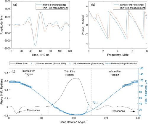
Figure 12c shows the variation in phase shift for shaft sensor 2 across one full rotation, sampled at the center frequency, 5 MHz. Annotated are the infinite-film and thin film regions. Within the thin-film region there is a steady increase in phase shift as the shaft and bearing surfaces converge, followed by a steady decrease as the surfaces diverge. Within the infinite film region, phase shift is constant except for two dips that correspond to the thickness at which the oil film resonates at 5 MHz, the index frequency. A modal average is taken over the infinite-film region to provide a reference.

Also shown in Fig. 12c are the corresponding film thickness measurements calculated using the phase shift and resonance methods. These highlight that the combination of ultrasonic methods can provide measurements in the thin- and thick-film regions of the bearing; however, there exists a gap between the measurement range of the two methods for intermediate film thicknesses. The precise range of this “blind spot” zone is related to transducer frequency and material properties.

Fig. 12c also shows a clear deviation between the expected and measured values within the diverging region, specifically between 210° and 250° shaft rotation angle in this example. This difference is due to cavitation (13) as air dissolved in the lubricant escape as bubbles in this low-pressure zone, causing the acoustic properties of the lubricant to change and scatter the ultrasonic signal. The existence of this cavitation region and measurement dead zone means that obtaining film thickness measurements around the full circumference using these methods is not practical. Thus, more than one sensor is required to continuously monitor film thickness if conditions are changing.

Figure 13 shows two examples of partial circumferential film thickness profiles under square wave loading, one at 50 kN peak load with a rotation speed of 60 rpm and one at 100 kN peak load with a rotation speed of 600 rpm. In both cases, load is applied for 180° and removed for 540°. Film thickness is calculated via the phase shift technique.

Figure 13. Circumferential film thickness under dynamic loading conditions, measured via shaft-mounted ultrasonic transducers using the phase shift technique. The operating conditions for these examples are (a) 60 rpm and 50 kN and (b) 600 rpm and 100 kN, both with a bearing temperature maintained at 50 °C.

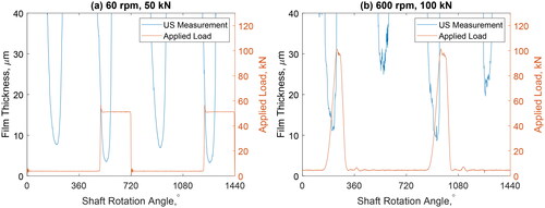
As expected, the minimum film is thinner for the 60 rpm case due to its lower Sommerfeld number. In both cases there is a substantial reduction in film thickness when the bearing is loaded compared to when it is unloaded. At 60 rpm the square wave loading patterns closely follow the desired input. However, at 700 rpm there is a significant rise time for the square wave loading pattern. This is because the valve does not close instantly and also because the oil is not perfectly incompressible. Although acceptable for this work, rise time could be mitigated in the future by reducing the hose length between the power pack and journal assembly, thus reducing the volume of the working fluid, or by using a faster acting valve.

Bearing sensor film measurements

The limitation with using shaft mounted sensors exclusively is that they cannot provide continuous minimum film measurements when operating conditions are rapidly changing. For example, if the load increases sharply when the shaft sensor is in the diverging region, cavitation effects will inhibit the shaft sensors from detecting a quantifiable change (13, 24). Thus, additional sensing hardware is required. For the current test platform, this is achieved with bearing-mounted ultrasonic transducers.

In this study, only the bearing sensors on the top face (unloaded region) and one side face were used, with the side face used only to determine minimum film thickness by triangulation. This side face corresponded to the converging region of the bearing. Outputs on the diverging side were deemed ineffectual due to cavitation effects. However, these unused sensors may be useful in the future, particularly if the rotation direction is reversed.

Examples of reflected time and frequency amplitude domain signal responses taken from top bearing sensor 2 are presented in Figs. 14a and 14b, respectively. These show a comparison between signals taken when the bearing is loaded and unloaded. Fig. 14b shows a dip in amplitude at a particular frequency; this corresponds to the resonant frequency of the oil layer. This frequency value can be applied to Eq. [2][2] $$f_m=\frac{cm}{2h},$$[2] to calculate film thickness.

Figure 14. (a) Example reflected signals in the time domain, taken from top bearing sensor 2. (b) Corresponding signals converted into the frequency amplitude domain. (c) Change in resonant dip frequency over four complete shaft rotations. Examples are taken from a square wave dynamic loading test case, with a shaft rotation speed of 100 rpm and bearing temperature of 50 °C.

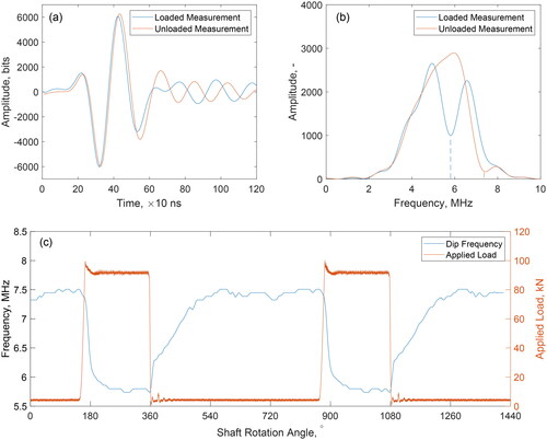
Fig. 14c shows the change in resonant dip frequency over four full rotations during a square wave dynamic loading test. A clear decrease in dip frequency is observed when load is applied, which corresponds to an increase in measured film thickness, although its rate of change is slower than the applied load profile. This is due to the squeeze film effect.

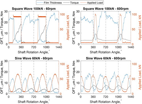
Figure 15 shows four examples of film thicknesses measured under dynamic loading conditions as captured by the top-mounted bearing sensors. These thicknesses were calculated via the film resonance technique, shown in Eq. [2][2] $$f_m=\frac{cm}{2h},$$[2] . Square wave and sine wave loading patterns across four full rotations at two different rotation speeds (60 and 600 rpm) are presented.

Figure 15. Comparison of film thickness at the top of the bearing (unloaded region) for four different dynamic loading cases, with variable load shape and rotation speed. Film measurements were taken via ultrasonic transducers mounted on the bearing top surface. Applied load measurements for each case are also shown.

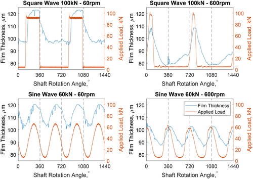
Examining these results, an increase in applied load leads to an increase in film thickness. This is because the top bearing sensors are located at the opposite side to the minimum film thickness region. Also, tests at higher rotation speeds demonstrate a consistently thinner film for the same reason. It should be noted that this measurement changes with load due to a change in both minimum film thickness and attitude angle.

For the square wave loading results, it is evident that film thickness takes time to reach equilibrium when the load is changed. This is due to the squeeze film effect, which means that the required volume of lubricant is unable to completely enter or exit the contact instantly. This effect is observed when the load is applied and removed. Squeeze film effects are less obvious for sine wave loading patterns due to their more gradual changes in load; however, a slight lag is still observed.

Comparing the squeeze time for square wave cases in Fig. 15, it appears that the film takes longer to recover when the load is reduced for the 60 rpm case than for the 600 rpm case. Although the 60 and 600 cases take similar angles of rotation to recover, on average 223° and 232°, respectively, this corresponds to a recovery time of 0.621 and 0.065s, respectively. It is thought that this difference is because a faster rotation speed may draw more lubricant into the contact, allowing the oil film to recover faster.

Figure 16 shows bearing film measurements for tests under the same square wave dynamic load but with different bearing temperatures, 50 and 70 °C. As expected, a higher temperature leads to a thicker measured film, which suggests a thinner minimum film on the opposite side of the bearing. Also, for the 100 rpm case, squeeze time is longer when the bearing temperature is at 50 °C than at 70 °C when the load is increased. On average, the loaded squeeze times are 0.28 and 0.23s, respectively. This trend is also observed when the load is removed, with a recovery time of 0.38 and 0.22s, for 50 and 70 °C, respectively. This is because a lower viscosity oil can enter and exit the contact more quickly when load conditions change.

Figure 16. Comparison of film thickness at the top of the bearing for dynamic loading cases with different bearing temperatures, 50 °C and 70 °C. (a) 100 rpm and (b) 700 rpm examples are provided. Film measurements are taken via ultrasonic transducers mounted on the bearing top surface. Applied load measurements for each case are also shown.

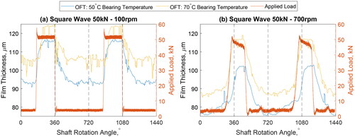
For the 700 rpm tests shown in Fig. 16, the loaded squeeze time is also significantly longer for the 50 °C case, at 0.031, compared to 0.023s at 70 °C. However, the average recovery times are very similar, at 0.055 and 0.056s, respectively. This could be due to the variable nature of the real system or because at higher speeds lubricant viscosity is less important in oil film recovery after a loading event.

Minimum film measurements

By applying the snapshot reference technique described previously shaft and top bearing sensor measurements can be combined to obtain a reference for the side bearing sensors, thus enabling continuous minimum film and attitude angle measurements. Figure 17 presents minimum film thickness and attitude angle measurements for four dynamic loading test cases: two square wave and two sine wave loading patterns, each at 60 and 600 rpm. These measurements are plotted against applied load.

Figure 17. Comparison of minimum film thickness and attitude angle for four different dynamic loading cases, with variable load shape and rotation speed. Film measurements are taken via ultrasonic transducers mounted on the top and side of the bearing. Applied load measurements for each case are also shown.

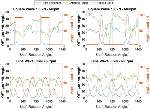
In Fig. 17, both minimum film thickness and attitude angle are consistently higher for the 600 rpm tests. As previously discussed, this is because expected because the resultant increased hydrodynamic pressure pushes the shaft and bearing surfaces apart with greater force.

A consistent decrease in film thickness is observed when applied load increases, with an obvious squeeze film effect causing the oil film to take time to change. The same can be seen for the attitude angle measurements, which tend towards equilibrium at the same rate.

Figure 18 shows the same film thickness and attitude angle data, although plotted against torque instead of the applied load. As expected, an increase in load leads to an increase in torque. Each test appears to be operating within the hydrodynamic regime, except the square wave 60 rpm test case when a load is applied. Torque is substantially higher for this test case compared to its 600 rpm counterpart. By considering the Stribeck curve, a lower rotation speed would only result in a higher torque if the system is operating within the mixed regime (25). In contrast, the 60 and 600 rpm sine wave tests are operating within the hydrodynamic regime, evidenced by the higher torque for the 600 rpm test.

Figure 18. Comparison of minimum film thickness and torque for four different dynamic loading cases, with variable load shape and rotation speed. Film measurements are taken via ultrasonic transducers mounted on the top and side of the bearing. Applied load measurements for each case are also shown.

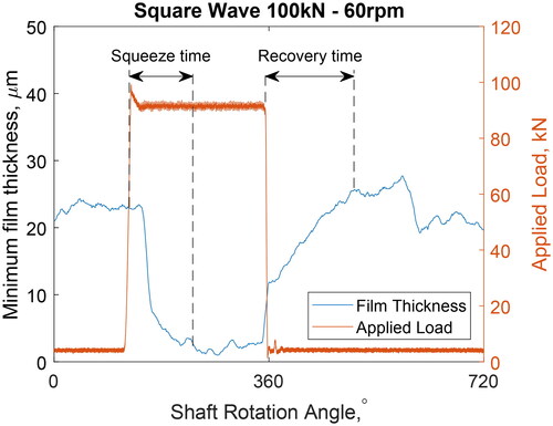
Squeeze time and recovery time are annotated in Fig. 19 as an example. In this, squeeze time is defined as the time taken for the oil film to reduce to within 5% of the mean final minimum film thickness when the load is applied, whereas recovery time is defined as the time taken for the oil film to increase to within 5% of the mean final minimum film thickness when the load is removed.

Figure 19. Measured minimum film thickness during a square wave dynamic loading test, with a peak load of 100 kN and shaft rotation speed of 60 rpm. Squeeze time and recovery time are annotated.

Figure 20 shows both squeeze and recovery time against rotation speed for two bearing temperatures, 50 °C and 70 °C, when subjected to a square wave applied load.

Figure 20. Comparison of (a) squeeze time and (b) recovery time for square wave dynamic loading test cases at 50 and 70 °C bearing temperature over a range of shaft rotation speeds between 80 and 700 rpm. Dashed lines correspond to power law curve fits.

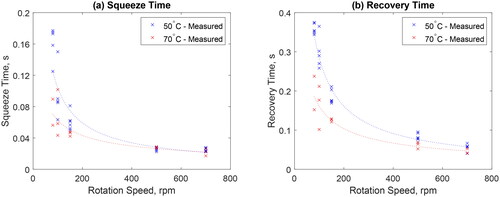
As expected, increased bearing temperature led to reduced squeeze and recovery times, particularly at lower rotation speeds, due to a reduced oil viscosity. A lower viscosity fluid has less resistance to flow and therefore can enter or exit the contact more easily. Figure 20 also shows that both squeeze time and recovery time reduce as rotation speed increases. With higher rotation speed, the lubricant is drawn into and out of the contact more rapidly, allowing film thickness to change more quickly.

Comparison with a numerical model

Minimum film thickness measurements were compared against predictions calculated via a numerical model. As previously discussed, even if a change in operating parameters, such as applied load, can be assumed to be instant, the change in film thickness is not. This is due to the squeeze film effect and can substantially increase complexity when attempting to model film behavior.

For simplicity, only square wave loading patterns were modeled in this study because these provide a region in which the film may reach equilibrium before the next loading or unloading instance. Minimum film thickness within each load state at equilibrium was calculated using the Raimondi-Boyd technique (26), and the change in film thickness between load states was predicted using a numerical technique presented by Jang and Khonsari (27). The results could then be combined to produce a continuous film thickness profile over multiple load cycles.

The squeeze film numerical technique requires the initial and final eccentricity ratios. These are calculated in this study via the Raimondi-Boyd technique (26). Then, small intervals between the initial and final eccentricity ratio values are created. In this case, steps of $\Delta \epsilon =0.01$ were found to be appropriate. At each interval, the corresponding dimensionless load capacity, $\overline{W}$, is calculated. This was achieved by solving the Reynolds equation for pressure and thereby dimensionless load capacity using a numerical solution provided by Jang and Khonsari (27). The value for dimensionless load capacity is then applied to the following equation to obtain the rate at which film thickness is changing, known as the approach velocity, V: [13] $$V=\frac{W{C}^3}{\mu rL\overline{W}},$$[13] where W is the applied load, C is the radial clearance, μ is the dynamic viscosity, r is the bearing radius, L is the bearing length, and $\overline{W}$ is the dimensionless load capacity.

Consequently, time duration, $\Delta t$, can then be calculated via the following: [14] $$\Delta t=\frac{2C({\epsilon }_2-{\epsilon }_1)}{V_1+V_2},$$[14] where ${\epsilon }_1$ and ${\epsilon }_2$ are the initial and final eccentricity ratios within that interval respectively. V₁ and V₂ are the initial and final approach velocities within that interval respectively. This process is repeated at every interval. The sum of all time duration values provides the total squeeze time.

This method requires assumptions to be made. In this case, these are as follows:

• The film thickness is small compared to other dimensions in the system, such as bearing diameter and length.

• The fluid is incompressible.

• The fluid is Newtonian.

• Fluid flow is laminar.

• Shaft and bearing deformation are negligible.

• Features such as oil ports and grooves are not considered.

It should be noted that this numerical model requires eccentricity ratio, rather than minimum film thickness as an input. However, a conversion between these parameters can be achieved by applying the following simple relationship: [15] $$h_{\mathit{min}}=C(1-\epsilon ).$$[15]

Two examples comparing numerical predictions against experimental results are presented in Fig. 21.

Figure 21. Comparison between experimental minimum film thickness measurements and a numerical prediction for two test cases under dynamic loading conditions. Measurements over four full rotations are presented. Operating conditions include a shaft rotation speed of 60 rpm (left) and 200 rpm (right), an applied square wave loading pattern with 100 kN peak load, and bearing temperature of 50 °C.

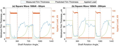
Assessing Fig. 21, the final experimental and predicted results are in good agreement during the loading part of the cycle. However, the difference between measured and predicted film thickness is generally greater when the bearing is unloaded. It is thought that this is due to the nonlinear relationship between operating conditions and film thickness. For example, it takes a far greater load increase to reduce film thickness from 3 to 2μm than it does to reduce from 20 to 19μm. The same is also true for rotation speed. Additionally, the phase shift technique is most accurate for thinner films.

Also, in many cases, when the load is removed, the measured film thickness peaks then settles down to a lower constant value. This was unexpected and was not predicted by the numerical model. There may be some form of bouncing effect as the load is quickly removed, although more work is required to confirm this.

For the 60 rpm test, a small delay between the load applied and the change in film thickness is present. This was also observed in a limited number of other test cases. The cause of this is uncertain. The feature could be due to a synchronisation error between data streams during either acquisition or processing; however, the change in film thickness when the load is removed initiates immediately.

The measured and predicted overall squeeze time and squeeze film profiles at low rotation speeds appear to be in good agreement; however, predicted overall recovery time is substantially longer than observed recovery time, as shown in Fig. 22. This compares squeeze and recovery time for a range of rotation speeds and peak applied loads. This figure also shows that predicted squeeze time at high rotation speeds is much longer.

Figure 22. Comparison of measured and predicted (a) squeeze times and (b) recovery times for square wave dynamic loading test cases, with peak loads of 50, 75, and 100 kN, over a range of rotation speeds between 80 and 700 rpm. Dashed lines correspond to power law curve fits.

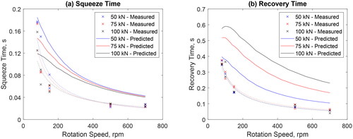
One of the key limitations of the numerical model is that it does not account for the oil groove, around the bearing circumference. With the inclusion of an oil groove the distance the lubricant must flow to exit the contact is reduced, because in effect the bearing length is smaller.

Small differences may also be due to the complex nature of a bearing experiencing dynamic loads. For example, even a small change in bearing temperature results in a substantial change in viscosity, which, as Eq. [13][13] $$V=\frac{W{C}^3}{\mu rL\overline{W}},$$[13] shows, would substantially affect approach velocity. Thus, the temperature profile around the entire bearing would be required for an optimum prediction. To achieve this, ambient temperature, how the fluid flows within the bearing, and effects due to oil ports must be known. This would also require a much more advanced numerical model than the one used in this study. This highlights the advantage of a robust measurement technique, which does not require such detailed knowledge of the system.

A weak correlation between applied load and squeeze time is observed in both the measured and predicted results, with a significant relationship (p < 0.05) observed in the measurements up to 150 rpm. Predicted recovery time is strongly related to applied load. However, there was no significant relationship found between observed recovery time and applied load.

Comparison with inductive sensor measurements

Film measurements via the ultrasonic technique were also compared against conventional inductive (gap) sensor measurements taken during testing. These inductive sensors were positioned at either side of the bearing in line with the top ultrasonic sensors, as indicated in Fig. 7. Gap sensor A is located on the motor side of the bearing, whereas gap sensor B is located on the slip-ring side.

Figure 23 compares film thickness measurements obtained by inductive sensors against ultrasonic measurements taken during a square wave loading cycle. In this test, the shaft rotation speed is 150 rpm and load varies between 5 and 25 kN. Loading frequency is 2.5 Hz, synchronized with the acquisition software’s internal clock rather than the encoder as done in previous experiments.

Figure 23. Comparison between ultrasonic and inductive gap sensor measurements on the test platform. Gap sensor A located on motor side of bearing; gap sensor B located on slip-ring side.

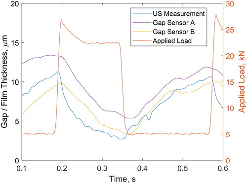
Gap sensors A and B both exhibit film thickness profiles similar to those of the ultrasonic measurements, although generally reporting a slightly thicker film. Also, gap sensor A and B measurements are somewhat inconsistent, even though previous experiments indicated that the shaft–bearing system was aligned, so results should be identical. As previously discussed, inaccuracies may be caused by shaft or bearing deformation. This is not accounted for due to the indirect nature of the inductive sensor measurement technique. Additionally, the voltage output of an inductive sensor is sensitive to changes in temperature. Although thermocouples were mounted in close proximity to the sensors and a careful pretest calibration was performed, uncertainties in temperature may still lead to reduced measurement accuracy.

Conclusion

The development of a novel bearing test platform and new ultrasonic referencing methods have enabled the study of lubricant films in journal bearings under dynamic loading conditions. This work has demonstrated that squeeze time reduces with decreasing oil viscosity, controlled via lubricant temperature. Squeeze time is also reduced with increased shaft rotation speed and applied load. Also, film recovery time was shown to reduce with increased shaft rotation speed.

These trends agree with numerical predictions; however, the measured squeeze and recovery times were significantly shorter, particularly at high rotation speeds, with actual recovery times up to four times faster at 700 rpm. This was due to the presence of an oil groove around the bearing circumference, which was not considered in the numerical model and would require a far more sophisticated predictive technique to include.

Results were also compared against conventional eddy current sensor measurements. Although there was reasonable agreement, shaft and bearing deformation introduced some uncertainty to the eddy current sensor measurements. This highlights the advantage of direct, non-invasive measurements offered by the ultrasonic method.

Nomenclature
ε	=	Eccentricity ratio
θ	=	Attitude angle (${}^{°}$ )
μ	=	Dynamic viscosity (Pas)
ρ	=	Density ($kg{m}^{-3}$ )
$\Phi$	=	Phase shift (rad)
$\varphi$	=	Bearing angle (${}^{°}$ )
$\phi$	=	Wave phase angle (rad)
ω	=	Attitude angle (${}^{°}$ )
C	=	Clearance (m)
c	=	Acoustic velocity ($m{s}^{-1}$ )
f	=	Wave frequency (Hz)
h	=	Film thickness (m)
K	=	Stiffness ($N{m}^{-1}$ )
L	=	Bearing length (m)
m	=	Resonance mode
r	=	Bearing radius (m)
t	=	Time (s)
V	=	Approach velocity ($m{s}^{-1}$ )
W	=	Applied load (N)
$\overline{W}$	=	Dimensionless load capacity ($\overline{W}$ )
z	=	Acoustic impedance (Rayl)

Acknowledgements

The authors are grateful to Dr. Henry Dodson, David Butcher, and Christopher Todd of the University of Sheffield for their help in the design and commissioning of the journal bearing test platform presented in this work.

Additional information

Funding

The authors are grateful to the Engineering and Physical Sciences Research Council for Prof. Rob Dwyer-Joyce’s fellowship on Tribo-Acoustic Sensors EP/N016483/1, the EPSRC Centre for Doctoral Training in Integrated Tribology EP/L01629X/1, and Sun Hydraulics for supplying components and technical support in the commissioning of the dynamic loading system.

References

- Malcolm, P. L. E. (2001), Understanding Journal Bearings, Applied Machinery Dynamics Co.: Durango, CO.
- Bhushan, B. and Dashnaw, F. (1981), “Material Study for Advanced Stern-Tube Bearings and Face Seals,” ASLE Transactions, 24(3), pp 398–409. doi:10.1080/05698198108983037
- Booser, R. E. (1997), Tribology Data Handbook, The Society of Tribologists and Lubrication Engineers: New York.
- Barrett, E. and Gunter, L. E. (1975), Steady-State and Transient Analysis of a Squeeze Film Damper Bearing for Rotor Stability, National Aeronautics and Space Administration: Washington, DC.
- Wang, D., Keith, T. G., Yang, Q., and Vaidyanathan, K. (2004), “Lubrication Analysis of a Connecting-Rod Bearing in a High-Speed Engine. Part I: Rod and Bearing Deformation,” Tribology Transactions, 47(2), pp 280–289.
- Waukesha Bearings. (2019), “Tilt Pad Journal Bearings.” Available at: https://www.waukbearing.com/en/engineered-fluid-film/product-lines/journal-bearings/tilt-pad-journal-bearings/ (accessed May 4, 2022).
- Gong, R. Z., Li, D. Y., Wang, H. J., Han, L., and Qin, D. Q. (2016), “Analytical Solution of Reynolds Equation under Dynamic Conditions,” Proceedings of the Institution of Mechanical Engineers - Part J: Journal of Engineering Tribology, 230(4), pp 416–427. doi:10.1177/1350650115604654
- Booker, J. F. (1965), “Dynamically Loaded Journal Bearings: Mobility Method of Solution,” Journal of Fluids Engineering, 87(3), pp 537–546. doi:10.1115/1.3650602
- Park, M., Jang, S., and Min, K. (2020), “Non-Newtonian Fluid Application of The Mobility Method in Engine Journal Bearing,” International Journal of Automotive Technology, 21(5), pp 1303–1313. 10.1007/s12239-012-0027-2.
- Mufti, R. A. and Priest, M. (2009), “Theoretical and Experimental Evaluation of Engine Bearing Performance,” Proceedings of the Institution of Mechanical Engineers - Part J: Journal of Engineering Tribology, 223(4), pp 629–644. doi:10.1243/13506501JET487
- Kataoka, T., Kikuchi, T., and Ashihara, K. (2011), “Measurement of Oil Film Thickness in the Main Bearings of an Operating Engine Using Thin-Film Electrode,” SAE International Journal of Fuels and Lubricants, 5(1), pp 425–433. doi:10.4271/2011-01-2117
- Moreau, H., Maspeyrot, P., Bonneau, D., and Frène, J. (2002), “Comparison between Experimental Film Thickness Measurements and Elastohydrodynamic Analysis in a Connecting-Rod Bearing,” Proceedings of the Institution of Mechanical Engineers - Part J: Journal of Engineering Tribology, 216(4), pp 195–208. doi:10.1243/135065002760199952
- Kasolang, S. and Dwyer-Joyce, R. S. (2008), “Observations of Film Thickness Profile and Cavitation around a Journal Bearing Circumference,” Tribology Transactions, 51(2), pp 231–245. 10.1080/10402000801947717.
- Ouyang, W., Zhou, Z., Jin, Y., Yan, X., and Liu, Y. (2020), “Ultrasonic Measurement of Lubricant Film Thickness Distribution of Journal Bearing,” Review of Scientific Instruments, 91, pp 065111. doi:10.1063/5.0007481
- Fillon, M. and Bouyer, J. (2004), “Thermohydrodynamic Analysis of a Worn Plain Journal Bearing,” Tribology International, 37(2), pp 129–136. doi:10.1016/S0301-679X(03)00051-3
- Welsh, J. (1983), Plain Bearing Design Handbook, Butterworth-Heinemann: Boston.
- Masuda, T., Ushijima, K., and Hamai, K. (2008), “A Measurement of Oil Film Pressure Distribution in Connecting Rod Bearing with Test Rig,” Tribology Transactions, 35(1), pp 71–76. doi:10.1080/10402009208982091
- Del Piezo. (2017), “Material Specification Sheet.” Available at: https://delpiezo.com/yahoositeadmin/assets/docs/MaterialSpecificationSheet.254613.pdf (accessed May 4, 2022).
- Matweb. (2018), “Morgan Advanced Ceramics Piezo Materials for Medical Devices PZT-5A Piezoceramic Material.” Available at: https://www.matweb.com/search/datasheet.aspx?matguid=7a480a939b39441ea856bc44623a76cc&ckck=1 (accessed May 4, 2022).
- Hunter, A., Dwyer-Joyce, R., and Harper, P. (2012), “Calibration and Validation of Ultrasonic Reflection Methods for Thin-Film Measurement in Tribology,” Measurement Science and Technology, 23(10), pp 105605. doi:10.1088/0957-0233/23/10/105605
- Drinkwater, B. W., Dwyer-Joyce, R. S., and Cawley, P. (1996), “A Study of the Interaction between Ultrasound and a Partially Contacting Solid–Solid Interface,” Proceedings of the Royal Society A: Mathematical, Physical and Engineering Sciences, 452(1955), pp 2613–2628.
- Yu, M., Shen, L., Mutasa, T., Dou, P., Wu, T., and Reddyhoff, T. (2020), “Exact Analytical Solution to Ultrasonic Interfacial Reflection Enabling Optimal Oil Film Thickness Measurement,” Tribology International, 151, pp 106522. doi:10.1016/j.triboint.2020.106522
- Reddyhoff, T., Kasolang, S., Dwyer-Joyce, R. S., and Drinkwater, B. W. (2005), “The Phase Shift of an Ultrasonic Pulse at an Oil Layer and Determination of Film Thickness,” Proceedings of the Institution of Mechanical Engineers - Part J: Journal of Engineering Tribology, 219(6), pp 387–400. doi:10.1243/135065005X34044
- Beamish, S., Li, X., Brunskill, H., Hunter, A., and Dwyer-Joyce, R. (2020), “Circumferential Film Thickness Measurement in Journal Bearings via the Ultrasonic Technique,” Tribology International, 148, pp 106295. https://linkinghub.elsevier.com/retrieve/pii/S0301679X20301377.
- Stachowiak, G. W. and Batchelor, A. W. (1993), Engineering Tribology, US: Butterworth-Heinemann.
- Raimondi, A. A. and Boyd, J. (1958), “A Solution for the Finite Journal Bearing and Its Application to Analysis and Design,” ASLE Transactions, 1(1), pp 159–174. doi:10.1080/05698195808972328
- Jang, J. Y. and Khonsari, M. M. (2015), “On the Characteristics of Misaligned Journal Bearings,” Lubricants, 3(1), pp. 27–53. doi:10.3390/lubricants3010027