HABSat-1: assessing the feasibility of using CubeSats for the detection of cyanobacterial harmful algal blooms in inland lakes and reservoirs

Abstract

Johansen RA, Beck R, Stumpf R, Lekki J, Tokars R, Tolbert C, McGhan C, Black T, Ma O, Xu M, Liu H, Reif M, Emery E. 2019. HABSat-1: assessing the feasibility of using CubeSats for the detection of cyanobacterial harmful algal blooms in inland lakes and reservoirs. Lake Reserv. Manage. 35:193–207.

The detection of cyanobacterial harmful algal blooms (CHABs) in freshwater lakes and reservoirs via satellite remote sensing remains a challenge. This is partially due to the spectral, spatial, and temporal configurations of most satellite imagers, which are designed for large terrestrial applications. This research evaluated the prelaunched performance of HABSat-1 for the detection of CHABs in inland waters. This study used the CASI hyperspectral airborne imager to mimic the potential configurations of the imager for HABSat-1. Synthetic HABSat-1 imagery was atmospherically corrected to reflectance, then used to evaluate the performance of 14 reflectance algorithms to estimate chlorophyll a (Chl-a), phycocyanin (PC), and the sum of pheophytin-corrected chlorophyll a and pheophytin a (SUMReCHL) concentrations. All algorithms use narrow spectral bands centered at 620 nm, 650 nm, 680 nm, and 708 nm, corresponding to important spectral reflectance features associated with CHABs. Eleven Chl-a and 10 PC algorithms performed well (r² > 0.7), indicating the configuration of HABSat-1 is well suited to the detection of CHABs in cyanobacteria-dominated waterbodies. The highest performing algorithms were the CI324 algorithm (ρ(680) – ρ(650) – (ρ(708) – ρ(650)) with an r² of 0.81, the 2B4D1 algorithm (ρ(650)/ρ(620)) with an r² of 0.844, and the NDCI41 algorithm (ρ(708) – ρ(620))/(ρ(708) + ρ(620)) with an r² of 0.755 for Chl-a, PC, and SUMReCHL. These promising results demonstrate that the use of relatively inexpensive customizable CubeSats coupled with simple reflectance-based algorithms is likely to be sufficient for the detection and estimation of CHABs in inland lakes and reservoirs.

Keywords:

• Chlorophyll a
• CubeSat
• cyanobacterial harmful algal bloom
• HABSat-1
• phycocyanin

Cyanobacterial harmful algal blooms (CHABs) are a serious environmental, human health, and economic concern that affect the United States and many other countries around the world (Anderson et al. 2000, Graham 2006, USEPA 2012a). High nutrient levels are known to adversely impact water quality and aid in the production of algal blooms, which have the potential to cause human illness and animal deaths (Linkov et al. 2009, USEPA 2012a, 2012b). Harmful blooms and poor water quality result in the loss of tens to hundreds of millions of dollars annually, due to lost revenue from the tourism, housing, and fishing industries. It is expected that these costs will continue to rise over the next couple decades, costing the United States billions of dollars (Anderson et al. 2000, Dodds et al. 2009).

CHABs are dynamic and respond rapidly to changes in the environment, such as water temperature, nutrient levels, and wind speed and direction, which vary on the order of days to even hours (Dokulil and Teubner 2000, Hunter et al. 2008). This creates an irregular distribution across the United States and makes the mapping and the prediction of the time and location of an event extremely difficult (Backer 2002, Stumpf et al. 2012). Given the uncertainty of the timing and location of blooms, satellite remote sensing is the preferred approach for regional monitoring of CHABs as it capitalizes on consistent orbits with large swath widths to provide near global coverage on a frequent basis when launched in sufficient numbers to combat cloud cover. Satellite remote sensing of CHABs is possible because algae and cyanobacteria have spectrally active pigments that produce unique spectral signatures detectable by the sensors (Christopher 2014). A specific focus has been placed on the pigments phycocyanin (PC) and chlorophyll a (Chl-a) as the most effective to estimate CHAB concentration (Schalles and Yacobi 2000, Simis et al. 2005, Randolph et al. 2008, Stumpf et al. 2016, Wozniak et al. 2016). PC is the cyanobacteria-specific pigment and is more useful for satellite mapping because it corresponds to the narrow spectral absorption feature at 620 nm produced by CHABs. Chl-a is the more ubiquitous pigment found in both cyanobacteria and algae. The spectral characteristics of Chl-a make it detectable via remotely sensed imagery for the mapping of most toxic and nontoxic algal blooms. However, Chl-a is especially useful for the detection of bloom conditions when algal communities contain multiple algal species. Most operational imaging satellites are unable to detect phycocyanin due to the lack of a narrow 620-nm spectral band associated with cyanobacteria. Others such as Landsat-8 are even unable to effectively quantify chlorophyll a due to wide near-infrared bands designed for land vegetation mapping (Hunter et al. 2008, Beck et al. 2016, Stumpf et al. 2016). A notable exception is Sentinel-2, which has proven to be very effective at detecting algal blooms including harmful algal blooms (HABs), although the lack of the critical PC band centered at 620 nm makes the detection of CHABs specifically less precise (Stumpf et al. 2016).

An additional concern is the spatial resolution of currently operational imagers, such as Sentinel-3, because their 300-m-on-a-side pixels are too coarse to be useful in small to mid-sized (<1000 ha) or narrow irregularly shaped waterbodies. The shape and size of a waterbody have significant influence on the ratio of pure to mixed pixels (that contain both terrestrial and aquatic elements), which subsequently influences the effectiveness of a sensor (Johansen et al. 2018a). More long-term studies are needed to evaluate and verify to what extent biophysical, atmospheric, and bloom conditions influence algorithm performance, because alterations in these conditions are likely to have significant effects to algorithm performance.

For these reasons, the use of small customized imagers on small satellites commonly known as CubeSats are proposed for detection and monitoring of CHABs in small to mid-sized freshwater lakes and reservoirs (>40 ha). CubeSats are relatively inexpensive and can be combined with low-cost spectrally customizable imagers, making them ideal for the detection of aquatic pigments that require specific narrow spectral bands (Wynne et al. 2008, Beck et al. 2016, Stumpf et al. 2016).

The aim of this article is twofold: to determine the most effective spectral band combination for the recently funded Harmful Algal Bloom Satellite-1 (HABSat-1), and to evaluate the potential of a HABSat-1 constellation for the detection and quantification of CHABs in small to mid-sized inland lakes and reservoirs. This was accomplished by using high-resolution airborne hyperspectral imagery to generate synthetic imagery that mimics the spectral and spatial configurations of HABSat-1. The synthetic imagery was then utilized to develop HABSat-1-specific algorithms to evaluate the performance of this sensor against coincident surface water observations.

Methods

Study area

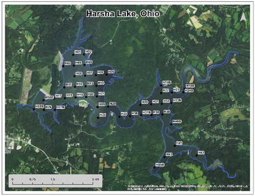
Harsha Lake (also known as East Fork Lake) is a 7.99-km² freshwater lake located in southwest Ohio, and it is affected by recent and reoccurring algal blooms (Fig. 1). Furthermore, Harsha Lake is a source of drinking water, contains beaches, and allows recreational fishing. Reservoirs with frequent blooms pose health risks to humans and wildlife as a result of exposure to the various toxins (i.e., dermatoxins, hepatoxins, and neurotoxins) produced by some algae at some times and locations (USEPA 2012a). Due to these factors, Harsha Lake is subject to routine monitoring by the US Environmental Protection Agency (USEPA) and US Army Corps of Engineers (USACE), which have provided a wealth of water quality data for this study.

Figure 1. Map of Harsha Lake near Cincinnati, Ohio with sampling scheme implemented on June 27th, 2014 in order to acquire water quality information from 44 sites within 1 h of image acquisition.

Datasets

The datasets used in this research were the Compact Airborne Spectrographic Imager (CASI) hyperspectral imagery (HSI) flown by the USACE Joint Airborne Lidar Bathymetry Technical Center of Expertise (JALBTCX) over Harsha Lake on 27 June 2014, and in situ measurements made using in vivo water sensors. The CASI imager was flown at an altitude of approximately 2000 m and acquired 48-band hyperspectral images. This flight plan resulted in the acquisition of images with swath widths of 1466 m and a spatial resolution of 1 m. The spectral resolution was over the wavelength range of 371 to 1042 nm, with a full width at half maximum (FWHM), or band width of 14 nm per band. The hyperspectral image was atmospherically corrected using Exelis Visual Information Solutions (ENVI) Fast Line of Sight Atmospheric Analysis of Hypercubes (FLAASH) module. For this study, it was found that the FLAASH atmospheric correction produced spectra visually similar to ASD spectroradiometer spectral measurements collected via boats within 1 h of the imagery acquisition (Figs. 2 and 3).

Figure 2. Averaged ASD surface relative reflectance spectra (red line) vs. Averaged CASI reflectance spectra (N = 16) (dotted blue line) for Harsha Lake with CASI data normalized to ASD at 550 nm. Wavelength in nm. They correspond well over the 425 and 865 nm wavelength range used in our study. One can even see a slight depression in the CASI spectra at 620 nm that corresponds to the phycocyanin absorption feature.

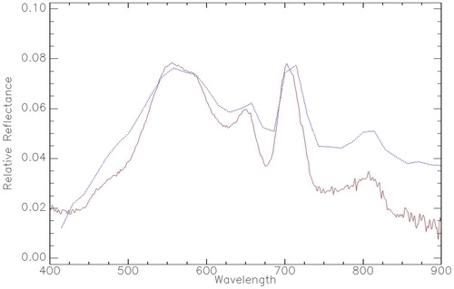
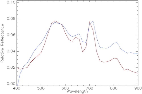
Figure 3. Averaged ASD surface relative reflectance spectra (red line) resampled to the same wavelengths as our CASI data vs. Averaged CASI reflectance spectra (N = 16) (dotted blue line) for Harsha Lake with CASI data normalized to ASD at 550 nm. Wavelength in nm.

In humid regions, such as the American Midwest, atmospheric correction may be difficult or even incomplete, but in this study a strong visual similarity was observed between the imagery reflectance and the ASD reflectance spectra. The correlations between the Chl-a indices and the coincident surface observations were also quite strong with Pearson’s r² values ranging from 0.6 to 0.7. The spectral similarity was also measured statistically following a method demonstrated in Beck et al. (2016, 2017).

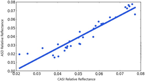
This method averaged 16 surface ASD and the CASI reflectance spectra, both corresponding to the same 16 sample locations on Harsha Lake. The CASI data were then normalized to the ASD surface spectral measurements using the Spectral Analysis and Management System (SAMS) software package at 550 nm (Fig. 2). This process was then reapplied so the average ASD reflectance spectra was normalized to the average CASI reflectance spectra at 550 nm (Fig. 3). Finally both sets of data (n = 32) were evaluated using linear regression and Pearson’s r², which demonstrated very high correlation with an r² value of 0.89 and a p value less than 0.001 (Fig. 4). There is some overestimation of CASI reflectance values, but the spectral signature correlates strongly enough with the ASD surface reflectance to provide confidence in the use of this atmospherically corrected CASI imagery for evaluating the HABSat-1 prototype.

Figure 4. Pearson’s test of linear correlation for ASD vs. CASI relative reflectance values at 32 wavelengths (n = 32). r² = 0.89, p < 0.001, degrees of freedom = 30, slope = 1.265, intercept = -0.024.

Both sets of reflectance spectral measurements (aircraft hyperspectral and surface field point spectra) provide the crucial spectral information required for the detection of CHABs from this sensor, which include the strong reflectance peak at 714 nm (Chl-a), the absorption features centered around 620 nm (phycocyanin), and the absorption feature at 680 nm corresponding to chlorophyll’s “red” absorption feature (Figs. 2 and 3).

The surface water sampling campaign for Harsha Lake included the use of 2 research boats to acquire coincident surface observations on a 400-m grid point spacing for both surface-water grab samples in conjunction with 2 cross-calibrated YSI brand water quality sondes. YSI sonde measurements were included in addition to traditional water grab techniques because sondes have been shown to provide a more standardized and efficient means of sampling with more consistent results. Sondes also require less sophisticated laboratory equipment and require minimal technical expertise as compared to traditional water sampling and laboratory analytical methods. The choice of surface observation method has been an issue for some researchers, so the YSI 6600 technical specifications are included here: range of ∼0–400 µg/L which equates to a range of 0–100 relative reflective units (RFU), a detection limit of ∼0.1 µg/L, resolution of 0.1 µg/L, and linearity/R² > 0.9999 (YSI 2003). Surface observation collection was coordinated with the imaging aircraft via an air-to-ground radio. Each boat’s crew collected the following:

1. Surface relative reflectance water grab samples from each of the sampling points were collected and analyzed for water quality constituents and algal pigments, and a subset of these points was processed for algae species identification and enumeration (I&E).

2. ASD relative reflectance spectra were captured to evaluate atmospheric correction of CASI imagery.

3. Sonde measurements collected during the campaign were chlorophyll a, phycocyanin, turbidity, specific conductance, pH, water temperature, and dissolved oxygen (YSI 2003).

4. GPS location and date/time-referenced photos of surface water conditions were taken at each sample point. All data were referenced to the WGS84 map datum and converted to the Universal Transverse Mercator (UTM) Zone 16 North map projection (Fig. 1).

Both sets of surface observations were used to evaluate the performance of simulated HABSat-1 satellite-derived algorithms for estimating the value of BGA/PC and chlorophyll a. The YSI measurements utilized the BGA/PC relative fluorescence unit (BGA_PC_RFU) and the Chl-a (µg/L) sensors, respectively (Stumpf et al. 2012, 2016). The YSI sonde measurements were corroborated by water grab sampling methods that measured chlorophyll a by extraction and spectrophotometric detection following the Standard Method 10200H2.b (APHA et al. 2012). Since remote sensing imagers detect total reflectance, for both chlorophyll a and its degradation products, the most appropriate measurement to compare ground truth would be to sum the equations for pheophytin (PE,a = 26.7[1.7 – (Abs665a) − (Abs664b)]) and pheophytin corrected chlorophyll a (CE,a = 26.7(Abs664b − Abs665a)) from Lorenzen (1967), abbreviated in this study as SUMReCHL (μg/L). These measurements calculate total chlorophyll pigment, which aligns more strongly with the in vivo reflectance of chlorophyll pigments measured by the imagers. Additionally, the algal I&E was completed following the Standard Method membrane filtration technique (APHA et al. 2012). Blue green algae/phycocyanin concentrations were not collected during the surface water grab campaign. Summary statistics for each set of the water surface observation measurements are shown (Table 1).

Table 1. Harsha Lake summary statistics for the 29 water quality sampling locations collected from the YSI water sonde and water grab surface measurements.

	Sampling technique	Minimum	Maximum	Mean	Std. dev.
SUMReCHL (μg/L))	Water grab	28.020	85.630	51.280	15.218
Chlorophyll a (µg/L)	YSI sonde	0.598	22.823	10.243	5.746
BGA/PC (RFU)	YSI sonde	3.702	26.645	10.901	4.713
Turbidity (NTU)	YSI sonde	8.608	26.940	14.456	3.540
Specific conductivity (S/cm)	YSI sonde	243.963	274.441	255.904	10.567
Water temperature (C)	YSI sonde	27.610	30.460	28.946	0.722
pH	YSI sonde	9.691	10.428	10.000	0.266
Dissolved oxygen (mg/L)	YSI sonde	12.979	21.781	16.791	2.736

HABSat-1

HABSat-1 is a recently funded prototype that will be launched as a low earth orbit (LEO) 3U CubeSat merged with a customized Sentera drone multispectral imager for the specific purpose of monitoring and detecting cyanobacterial harmful algal blooms. The goal of HABSat-1 is to monitor CHABs at roughly 1/100th to 1/1000th of the cost of current long-life imaging satellites such as MERIS, Sentinel-3 (OLCI), or Sentinel-2. The use of numerous low-cost satellites offers reduction to overall cost and risk of individual satellite failure. This method uniquely offers the temporal, spectral, and spatial resolutions needed for the study of CHABs, especially in small inland lakes and reservoirs (Beck et al. 2016, 2017, Johansen et al. 2018a). One goal of this article was to determine the optimal spectral band selection for HABSat-1 by testing various band configurations coupled with various Chl-a/PC algorithms. The best spectral combination will ultimately be incorporated on HABSat-1, which is scheduled to launch in late 2021.

Given that the satellite is still in the prelaunch stage there are some unknowns, but the proposed satellite will ideally follow an orbital inclination of approximately 51.6 degrees and an orbital altitude of approximately 450 km. This would result in an orbit around the earth roughly every 90 minutes, which would potentially provide 215 passes over our notional Ohio target each year, assuming off-nadir pointing. These estimates are optimistic, given that the number of overpasses is dependent on the actual orbit, which will be dictated by NASA, and off-nadir imaging will not be used routinely, but instead as a just-in-case capability. That being said, the acquisition of nadir imagery of our Ohio target would be significantly less at an estimated 15–16 per year per satellite.

Given these specifications, the revisit time will depend upon the exact altitude of the imager and latitude of the location being observed. National Aeronautics and Space Administration (NASA) guidelines predict an operational life span between 1 and 2 yr that will ensure that the satellite deorbits within 25 yr. Regardless of the final details of what will probably be an opportunistic launch, HABSat-1 is a prototype for a constellation of low-cost CubeSats consisting of a mix of both near-equatorial and near-polar orbits in order to maximize coverage and to mitigate frequent cloud cover in order to improve HAB monitoring for lakes and reservoirs globally.

The HABSat-1 Sentera Quad multispectral imager is a customized 4-band sensor with the following characteristics: sensor width of 4.8 mm, sensor height of 3.6 mm, focal length of 25 mm (as customized for HABsat-1), image width of 1248 pixels, and image height of 950 pixels (Sentera 2018). These specifications allow for an estimated spatial resolution of 72.5 m. Its prelaunch and postlaunch signal-to-noise ratios with its new lenses will be determined by NASA. The image footprint will be approximately 86.4 × 64.8 km, which is more than sufficient to provide complete coverage of most small to mid-sized lakes and reservoirs (>40 ha), which can range from a few hectares to thousands. Due to this relatively small footprint size, CHAB coverage in large water bodies such as the Great Lakes will be limited. The spectral configuration is customizable from wavelengths of 400 to 900 nm with band widths of approximately 10–20 nm. The band configuration and selection process are discussed later.

HABSat-1 spectral configuration

The Sentera Quad multispectral imager was chosen as a cost-effective alternative to developing an entirely new sensor. The adaption of a commercial unmanned aerial vehicle (UAV) product is attractive because it is customizable, product tested, and relatively inexpensive. This approach significantly outweighs the cost associated with the development of a new imager. Although the Sentera Quad is limited to only 4 spectral bands, the manufacturer is willing to outfit its imager with a wide selection of custom narrow-band filters. Therefore, a process was developed to select the most appropriate wavelengths for each band. This was initially done by evaluating the important spectral components of CHABs and the optical methods used for their detection (Kahru and Brown 1997, Wynne et al. 2008, Ogashawara et al. 2013). We then simulated the prelaunch imagery from real hyperspectral imagery acquired over Harsha Lake with appropriate water truth to test a variety of algorithms with this approximation of the real HABSat-1 imager.

The literature review revealed a few bands of primary significance, including the narrow bands located at 620 nm and 650 nm, which correspond to the minimum and maximum reflectance features of phycocyanin (Ogashawara et al. 2013). Another critical band is centered at 708 nm, caused by the backscattering of cyanobacteria (Wynne et al. 2008, 2012). These 3 bands are the spectral features directly associated with cyanobacteria and freshwater CHABs. Another important wavelength was the chlorophyll “red” absorption feature near 680 nm, which is utilized to differentiate CHABs from other types of aquatic pigments (Wynne et al. 2008). Additional consideration was given to the green band at 560 nm, which also serves as a chlorophyll reflectance peak (Zhao et al. 2010). For completeness, the blue band centered at 490 nm for true color and the near-infrared band near 750 nm for delineation between terrestrial and aquatic vegetation were also evaluated. Due to the 4-band limit of the Sentera Quad sensor, we evaluated these 7 narrow spectral bands (490 nm, 560 nm, 620 nm, 650 nm, 680 nm, 708 nm, 750 nm) and selected the band combination that enabled the highest performing algorithms. It is acknowledged that the list of potential bands wasn’t exhaustive, nor was the list of potential algorithms, but the band centers were carefully chosen from searches of the literature (Beck et al. 2016, 2017, 2018, Johansen et al. 2018a, Mishra and Mishra 2014, Stumpf et al. 2016, Wynne et al. 2008). For the prelaunch simulation, the final ideal spectral configuration for HABSat-1 was chosen to be 620 nm, 650 nm, 680 nm, and 708 nm, each with FWHM band width of 28 nm, and a ground sampling distance (GSD) spatial resolution of 72 m (Table 2). The final band selection on the real imager will be adjusted to use the available spectral filters. The actual GSD will be determined after HABSat-1 is launched, but preliminary estimates are between 70 and 90 m.

Table 2. Sensor configurations for the future HABSat-1 and the hyperspectral derived synthetic HABSat-1

	HABSat-1		Synthetic HABSat-1
Bands	Center	FWHM	Synthetic center	FWHM
	(nm)	(nm)	(nm)	(nm)
B1	620	15	622.2	28
B2	650	15	650.6	28
B3	680	15	679.1	28
B4	708	15	707.5	28

Synthetic HABSat-1 and imagery analysis

In order to produce the synthetic HABSat-1 configurations from Table 1, the original airborne CASI hyperspectral imagery was spectrally averaged by applying equal weight band math using the raster and waterquality packages in R (Hijmans 2016, Johansen et al. 2018b, R Core Team 2017). After spectral averaging, these data were spatially resampled from the original 1-m resolution of CASI to the 72-m GSD spatial resolution of HABSat-1. This method of spectral binning and spatially resampling hyperspectral imagery to mimic coarser sensors, recommended by Broge and Mortensen (2002), has been successfully applied to MERIS (Koponen et al. 2002), and expanded to include WorldView-2, Sentinel-2, Landsat-8, and Moderate Resolution Imaging Spectroradiometer (MODIS) by Beck et al. (2016). This approach has been documented to introduce relative errors on the order of 6–8% during the linear spectral binning and 10–32% during the spatial resampling process (Schlapfer et al. 1999, 2002). An alternative approach, which many researchers have followed, is to utilize surface measurements acquired from portable or handheld spectroradiometers (Mittenzwey et al. 1992, Koponen et al. 2002, Augusto-Silva et al. 2014). However, this research follows the methodology established by previous studies where airborne hyperspectral imagery was used in lieu of spectroradiometer surface measurements (Beck et al. 2016, Johansen et al. 2018a). Reif (2011) has detailed the advantages of this method, which include increased spatial and temporal coverage coupled with a reduction in time and labor costs. Additional consideration should be given to lake geometry because many inland lakes and reservoirs are irregularly shaped, making the acquisition of pure water pixels challenging in narrow or river-like water bodies. It is suggested based on previous studies that a minimum of 10 well-distributed pure water pixels (pixels that do not contain any land, clouds, or anthropogenic elements) is critical for evaluating the algorithm performance for any individual waterbody (Stone 1974, Picard and Cook 1984). Twenty-nine (n = 29) pure water pixels were used to evaluate the band selection/algorithm index combinations used in this study. Table 2 displays the original (proposed) and synthetic (CASI-derived) band configurations of the HABSat-1 sensor.

After the synthetic imagery is created, a host of chlorophyll a and BGA/PC algorithms may be calculated from those data. These algorithm indices were then tested against water truth data to evaluate their performance. Previous work by Beck et al. (2016, 2017) and Johansen et al. (2018a) has guided HABSat-1 specific variations based on of the well-established 2-band difference algorithms (Schalles and Yacobi 2000, Mishra et al. 2009, Beck et al. 2017), 3-band difference algorithms (Dekker 1993, Mishra and Mishra 2014), 2-band subtraction algorithms (Amin et al. 2009, Beck et al. 2017), normalized difference chlorophyll a/cyanobacterial indices (Mishra and Mishra 2014), and cyanobacterial indices (Wynne et al. 2008). After the removal of any mixed pixels (land, clouds, or man-made objects), there were 29 pure water pixels available to consider in the evaluation of algorithm values against the corresponding YSI sonde collected surface measurements for chlorophyll a and BGA/PC, as well as the water grab samples used to calculate SUMReCHL.

Algorithm evaluation and model validation

The standard Type-1 linear regression test was used to compare the 29 surface observations for the YSI collected Chl-a-µg/L and BGA/PC (RFU) and the water grab samples measured as SUMReCHL, which correspond to the cloud-free pure water pixels for each of the algorithm indices (YSI 2003). Each set of algorithm index derived pixel values and surface observations was evaluated using the Pearson’s r² correlation, p value, slope, and intercept and are shown under the global model heading of Tables 3–5. For further comparison and model validation a robust repeated k-fold cross-validation method was applied for each algorithm and surface observation data combination (Stone, 1974, Picard and Cook, 1984). Given that the data set contained 29 observations, it was decided a threefold approach was the most appropriate. The k-fold method divides the entire set of observations (n = 29) into 3 stratified random groups. Two groups, or two-thirds of the samples, are used for the model calibration, while the remaining group, one-third of the samples, is used for the validation. This calibration–validation process is then repeated, so each of the possible combinations of 2 group calibration to 1 group validation is calculated, which results in a total of 3 model runs. To reduce the effect of outliers and sampling bias, this entire process is then iterated 4 more times, where in each new iteration the groups are randomly populated with a new subset of the original 29 observations. The repeated k-fold method utilizes all 15 models (3 k-fold model multiplied by 5 iterations), to produce an average r², root mean square error (RMSE), r², and mean average error (MAE) for each of the water quality algorithms. This robust cross-validation technique is used to measure the accuracy of each chlorophyll a and BGA/PC algorithm and provides a standardized comparison of performance between algorithms (Tables 3–5).

Table 3. HABSat-1 algorithm calculations and evaluation against in situ surface observation of YSI sonde derived chlorophyll-a values for all 29 surface water observations (Global Model), and the average of the 15 k-folds models Cross-Validated Average).

		Global model				Cross–validated average
Algorithms	Band math (wavelength, nm)	r²	Slope	Intercept	p Value	r²	RMSE	MAE
2BSub algorithms
2B2Sub1	(650 – 620)	0.457	0.370	11.845	0.000	0.478	4.246	3.337
2B4Sub1	(708 – 620)	0.735	0.080	7.779	0.000	0.761	3.052	2.498
2B4Sub2	(708 – 650)	0.729	0.092	7.022	0.000	0.747	3.066	2.485
2BDA algorithms
2B4D1	(708/620)	0.708	31.268	–23.345	0.000	0.753	3.246	2.674
2B2D1	(650/620)	0.471	147.669	–135.735	0.000	0.510	4.248	3.358
2B4D3	(708/680)	0.763	32.684	–31.380	0.000	0.787	2.955	2.430
2B4D2	(708/650)	0.698	36.278	–29.088	0.000	0.724	3.272	2.679
NDCI algorithms
NDCI41	(708 – 620)/(708 + 620)	0.714	69.338	8.114	0.000	0.735	3.153	2.581
NDCI21	(650 – 620)/(650 + 620)	0.469	291.966	11.976	0.000	0.504	4.214	3.232
NDCI43	(708 – 680)/(708 + 680)	0.749	84.451	0.411	0.000	0.768	2.862	2.332
NDCI42	(708 – 650)/(708 + 650)	0.696	80.061	7.307	0.000	0.703	3.217	2.634
CI algorithms
CI324	(680 – 650 – (708 – 650))	0.788	–0.089	2.002	0.000	0.810	2.698	2.199
3BDA algorithms
3BDA431	((708 – 680) × 620)	0.795	0.000	2.575	0.000	0.802	2.587	2.070
3BDA421	((708 – 650) × 620)	0.754	0.000	6.910	0.000	0.774	2.917	2.364

Table 4. HABSat-1 algorithm calculations and evaluation against in situ surface observation of YSI sonde derived BGA/PC units for all 29 surface water observations (Global Model), and the average of the 15 k-folds models (Cross-Validated Average).

		Global model				Cross–validated average
Algorithms	Band math (wavelength, nm)	r²	Slope	Intercept	p Value	r²	RMSE	MAE
2BSub algorithms
2B2Sub1	(650 – 620)	0.625	0.354	12.437	0.000	0.628	3.019	2.374
2B4Sub1	(708 – 620)	0.822	0.069	8.764	0.000	0.833	2.112	1.709
2B4Sub2	(708 – 650)	0.789	0.078	8.152	0.000	0.815	2.333	1.965
2BDA algorithms
2B4D1	(708/620)	0.829	27.744	–18.902	0.000	0.844	2.070	1.662
2B2D1	(650/620)	0.471	147.669	–135.735	0.000	0.510	4.248	3.358
2B4D3	(708/680)	0.717	25.991	–22.199	0.000	0.756	2.611	2.079
2B4D2	(708/650)	0.783	31.525	–23.277	0.000	0.788	2.359	1.896
NDCI algorithms
NDCI41	(708 – 620)/(708 + 620)	0.795	60.041	9.058	0.000	0.819	2.271	1.783
NDCI21	(650 – 620)/(650 + 620)	0.624	276.159	12.541	0.000	0.627	3.002	2.329
NDCI43	(708 – 680)/(708 + 680)	0.690	66.463	3.163	0.000	0.741	2.711	2.143
NDCI42	(708 – 650)/(708 + 650)	0.751	68.199	8.400	0.000	0.775	2.487	1.975
CI algorithms
CI324	(680 – 650 – (708 – 650))	0.714	–0.070	4.465	0.000	0.737	2.731	2.210
3BDA algorithms
3BDA431	((708 – 680) × 620)	0.644	0.000	5.242	0.000	0.679	2.882	2.320
3BDA421	((708 – 650) × 620)	0.768	0.000	8.141	0.000	0.800	2.476	2.025

Table 5. HABSat-1 algorithm calculations and evaluation against surface water grab derived SUMReCHL units for all 29 surface water observations (Global Model), and the average of the 15 k-folds models (Cross-Validated Average).

		Global model				Cross–validated average
Algorithms	Band math (wavelength, nm)	r²	Slope	Intercept	p Value	r²	RMSE	MAE
2BSub algorithms
2B2Sub1	(650 – 620)	0.430	0.962	55.452	0.000	0.456	12.249	10.078
2B4Sub1	(708 – 620)	0.731	0.214	44.686	0.000	0.723	7.868	5.785
2B4Sub2	(708 – 650)	0.731	0.246	42.623	0.000	0.735	7.979	5.963
2BDA algorithms
2B4D1	(708/620)	0.730	85.194	–40.234	0.000	0.736	7.904	5.846
2B2D1	(650/620)	0.439	383.024	–327.355	0.000	0.457	11.567	9.350
2B4D3	(708/680)	0.700	84.064	–55.774	0.000	0.711	8.562	6.475
2B4D2	(708/650)	0.724	99.163	–56.225	0.000	0.714	8.185	6.235
NDCI algorithms
NDCI41	(708 – 620)/(708 + 620)	0.725	187.585	45.521	0.000	0.755	7.868	5.898
NDCI21	(650 – 620)/(650 + 620)	0.434	753.917	55.757	0.000	0.444	11.790	9.563
NDCI43	(708 – 680)/(708 + 680)	0.692	217.900	25.911	0.000	0.704	8.437	6.368
NDCI42	(708 – 650)/(708 + 650)	0.720	218.503	43.267	0.000	0.739	8.060	6.131
CI algorithms
CI324	(680 – 650 – (708 – 650))	0.712	–0.227	30.254	0.000	0.733	8.519	6.348
3BDA algorithms
3BDA431	((708 – 680) × 620)	0.671	0.001	32.375	0.000	0.687	9.093	6.727
3BDA421	((708 – 650) × 620)	0.719	0.001	42.542	0.000	0.742	8.192	6.064

Results

The goal of this research was to evaluate the performance of an approximation of the future HABSat-1 imaging satellite for the detection and monitoring of CHABs in small to mid-sized lakes and reservoirs. This was accomplished using simple relative reflectance-based algorithms designed to detect and estimate the concentrations of both the ubiquitous chlorophyll pigment and the cyanobacterial-specific pigment phycocyanin. Each algorithm was evaluated against both pigments because varying conditions and algal dominance may influence which algorithm should be applied (Stumpf et al. 2016). Given that this sensor was designed specifically for the detection of algal blooms, it is expected that most of the test algorithms would have strong correlations and low root mean square error (RMSE). For that reason, the algorithms deemed acceptable are those with the highest performance, which for this study was considered an average cross-validated r² value of greater than 0.7 (Tables 3–5).

Chlorophyll a algorithms

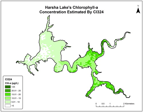
Eleven of the 14 HABSat-1 algorithms tested produced correlations sufficient for the detection of chlorophyll a with r² values from 0.703 to 0.810 and RMSEs from 2.587 to 3.272 with the proposed HABSat-1 imager band selection (620 nm, 650 nm, 680 nm, 708 nm). The chlorophyll a values ranged from 0.598 to 22.823 (µg/L) from the surface observations, which gives a relative RMSE of 0.116 to 0.146 (Table 3). The 3 algorithms that did not meet the threshold were 2B2Sub1 (ρ(650) – ρ(620)), 2B2D1 (ρ(650)/ρ(620), and NDCI21 (ρ(650) – ρ(620))/(ρ(650) + ρ(620)), which demonstrates the lack of spectral response in the 650-nm band. There is little variation between the performances of the chlorophyll a algorithms, regardless of the type of algorithm, likely due to spectral influence chlorophyll a especially on band 5 centered at 708 nm. The best performing algorithm for chlorophyll a was the CI324 (ρ(680) – ρ(650)) – (ρ(708) – ρ(650)) algorithm with an average r² of 0.810 and an RMSE of 2.698 (Fig. 5).

Figure 5. Results of the best performing Chl-a algorithm, CI324, with darker pixels indicating higher Chl-a concentrations. Pearson's r² = 0.81 of and a RMSE of 2.587.

BGA/PC algorithms

Ten of the 14 algorithms had strong correlations with the sonde-measured BGA/PC considered acceptable for this study, with r² values ranging from 0.737 to 0.844 and RMSE values from 2.070 to 2.731. The BGA/PC values ranged from 3.702 to 26.645, corresponding to a relative RMSE error of 0.09 to 0.119, which is slightly better than the chlorophyll a algorithms (Table 4). The higher performance of BGA/PC algorithms is logical, given the dominance of cyanobacteria at the time of this study. These finding are confirmed by the algal species identification and enumeration (I&E), which found that cyanobacterial species made up more than 97% of the relative abundance of algae in Harsha lake at the time of this study (Table 6). The 4 algorithms that did not met the performance criteria were 2B2Sub1 (ρ(650) – ρ(620)), 2B2D1 (ρ(650)/ρ(620)), NDCI21 (ρ(650) – ρ(620))/(ρ(650) + ρ(620)), and 3BDA431 (ρ(708) – 680)) × ρ(620)), again suggesting that the 650-nm band has a lower spectral response than the other 3 bands. However, these algorithms had stronger correlations with BGA/PC than with chlorophyll a. The best performing PC algorithm was the 2B4D1 (ρ(708)/ρ(620)) with an average r² 0.844 of and an RMSE of 2.070 (Fig. 6). It was expected that the BGA/PC algorithms would perform slightly better than the chlorophyll a algorithms because Harsha Lake was heavily dominated by cyanobacteria at the time of this study (Johansen et al. 2018). Of specific interest are the BGA/PC algorithms with r² values of greater than 0.8, which make use of the 708-nm band and 620-nm band, most closely associated with Chl-a and PC concentrations.

Figure 6. Results of the best performing PC algorithm, 2B4D1, with darker pixels indicating higher PC concentrations. Pearson's r² = 0.844 of and a RMSE of 2.07.

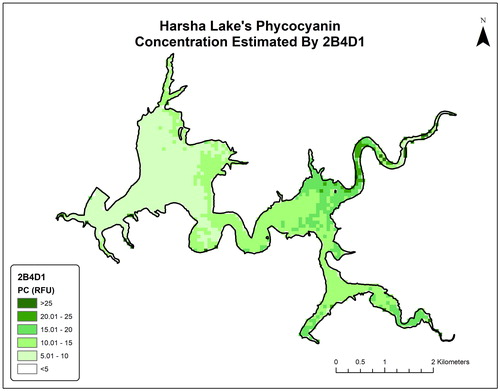
Table 6. Algae taxonomy of Harsha Lake measured in average relative abundance by algae divisions.

Algae division	Average relative abundance (%)
Bacillariophyta	0.08
Chlorophyta	1.06
Chrysophyta	0.00
Cryptophyta	1.53
Cyanobacteria	97.32
Euglenophyta	0.00
Pyrrophyta	0.02
Total	100.00

SUMReCHL algorithms

The water grab samples produced results similar to the YSI measurements, with 10 of the 14 algorithms having correlations sufficient for the detection of chlorophyll a as measured by SUMReCHL. These algorithms had average r² values ranging from 0.704 to 0.755 and RMSEs from 7.868 to 8.562. The SUMReCHL values ranged from 28.020 to 85.630 (µg/L) from the surface observations, which gives a relative RMSE of 0.136 to 0.148 (Table 5). There is an overall slightly lower correlation between the HABSat-1 algorithms and the water grab samples compared to the YSI measurements. However, the algorithms perform well and remain fairly consistent for both metrics of chlorophyll, with one additional algorithm, 3BDA431 (ρ((708) – ρ(680)) × ρ(620)), performing just below the study threshold of r² 0.7. The best performing algorithm for SUMReCHL was the NDCI41 (ρ(708) – ρ(620))/(ρ(708) + ρ(620)) algorithm with an average r² of 0.755 and an RMSE of 7.868.

Discussion

This research utilized atmospherically corrected airborne hyperspectral imagery to develop a synthetic approximation of a soon-to-launch multispectral satellite imager specifically designed for the detection and monitoring of cyanobacterial harmful algal blooms in small to mid-sized lakes and reservoirs. The authors refined and evaluated 14 HAB algorithms that make use of 4 spectral features associated with chlorophyll a and phycocyanin, which are the 2 main pigments used for the remote sensing of CHABs. The algorithm performances follow previous work closely, with the best algorithms making use of the 708-nm chlorophyll band and the well-known PC absorption feature centered around 620 nm. It should be noted that this work did not evaluate every possible combination of band math when developing the algorithms, but from searching the literature the 14 chosen appeared to cover the vast majority of variations. In addition, 11 Chl-a, 10 BGA/PC, and 10 SUMReCHL algorithms had strong correlations coupled with relatively low RMSEs, which are considered sufficient enough for the estimation of these pigments and subsequently usable as proxies for HAB concentration (Tables 3–5). It is still unknown how this sensor will perform on detecting other algal blooms in waters less dominated by cyanobacteria, but HABSat-1 shows significant potential for the monitoring of cyanobacteria-dominated waters like Harsha Lake.

Under the specific biophysical conditions of the study, our findings demonstrated a high level of confidence in the ability of HABSat-1 to be able to not only detect algal blooms but estimate the concentrations of chlorophyll a and phycocyanin with the precision needed to assist water managers in evaluating water quality. More research will be needed once HABSat-1 launches to evaluate the exact slopes, intercepts, and errors associated with the sensor. Preliminary simulations suggest that this project will fill a major water quality research gap, by being a prototype for the use of constellations of CubeSats as a cost-effective alternative for the near real-time monitoring small to mid-sized water bodies. If HABSat-1 is a success, it would provide a case study and provide the way for the use of constellations of small custom-designed CubeSats, which would eliminate some of the issues associated with traditional satellite imagers, mainly the trade-offs between temporal, spectral, and spatial resolutions. Ideally, CubeSats such as HABSat-1 will be launched in swarms of 4–16 to improve temporal coverage to daily or once every few days instead of the current 10-day return time of each Sentinel-2A and Sentinel-2B, which are currently the only open-source imagers available with the spectral and spatial resolution capable of detecting CHABs in small to mid-sized water bodies. HABSat-1 will not launch until late 2021, but if successful will be a significant step forward in the ability to systematically monitor water quality in small water bodies across large geographic regions.

Acknowledgments

We thank the University of Cincinnati’s Library’s Research and Data Services and the University of Cincinnati’s CubeCats, which provided valuable technical support and expertise. Any use of trade, product, or firm names is for descriptive purposes only and does not imply endorsement by the U.S. government. This article expresses only the personal views of the authors and does not necessarily reflect the official positions of NASA, the Corps of Engineers of the Department of the Army, or NOAA.

References

- Amin R, Zhou J, Gilerson A, Gross B, Moshary F, Ahmed S. 2009. Novel optical techniques for detecting and classifying toxic dinoflagellate Karenia brevis blooms using satellite imagery. Optics Express. 17(11):1–13.
- Anderson DM, Hoagland P, Kaoru Y, White AW. 2000. Estimated annual economic impact from harmful aglal blooms (HABs) in the United States. Woods Hole (MA): Woods Hole Oceanographic Institution.
- [APHA] American Public Health Association, [AWWA] American Water Works Association, [WEF] Water Environment Federation. 2012. Standard methods for examination of water and wastewater, 22nd ed. Washington (DC).
- Augusto-Silva PB, Ogashawara I, Barbosa CCF, de Carvalho LAS, Jorge DSF, Fornari CI, Stech JL. 2014. Analysis of MERIS reflectance algorithms for estimating chlorophyll-a concentration in a Brazilian reservoir. Remote Sensing. 6: 11689–117077. doi:10.3390/rs61211689.
- Backer LC. 2002. Cyanobacterial harmful algal blooms: developing a public health response. Lake Reserv Manage. 18(1):20–31. doi:10.1080/07438140209353926.
- Beck RA, Liu H, Johansen R, Xu M, McGhan C, Black GT, Ma O, Tolbert C, Lekki J, Tokars R, et al. 2018. Adapting low-cost technology to CubSats for environmental monitoring and management: Harmful Algal Bloom Satellite-1 (HABSat-1). 32nd Annual AIAA/USU Conference on Small Satellites Proceedings. https://digitalcommons.usu.edu/smallsat/2018/all2018/486
- Beck RA, Xu M, Zhan S, Liu H, Johansen RA, Tong S, Yang B, Shu S, Wu Q, Wang S, et al. 2017. Comparison of satellite reflectance algorithms for estimating phycocyanin values and cyanobacterial total biovolume in a temperate reservoir using coincident hyperspectral aircraft imagery and dense coincident surface observations. Remote Sens. 9:538. doi:10.3390/rs9060538.
- Beck RA, Zhan S, Liu H, Tong S, Yang B, Xu M, Ye Z, Huang Y, Wu Q, Wang S, et al. 2016 Comparison of satellite reflectance algorithms for estimating chlorophyll-a in a temperate reservoir using coincident hyperspectral aircraft imagery and dense coincident surface observations. Remote Sens Environ. 178:15–30.
- Broge NH, Mortensen JV. 2002. Deriving green crop area index and canopy chlorophyll density of winter wheat from spectral reflectance data. Remote Sens Environ. 81:45–57. doi:10.1016/S0034-4257(01)00332-7.
- Christopher N. 2014. Algae, phytoplankton and chlorophyll. Fundamentals of environmental measurements. Fondriest Environmental, Inc. http://www.fondriest.com/environmental-measurements/parameters/water-quality/algae-phytoplankton-and-chlorophyll
- Dekker AG. 1993. Detection of optical water quality parameters for eutrophic waters by high resolution remote sensing [thesis]. Amsterdam, The Netherlands: Vrije Universiteit.
- Dodds WK, Bouska WW, Eitzmann JL, Pilger TJ, Pitts, KL, Riley AJ, Schlosser JT, Thornbrugh DJ. 2009. Eutrophication of U.S. freshwaters: analysis of potential economic damages. Environ Sci Technol. 43(1):12–19. doi:10.1021/es801217q.
- Dokulil MT, Teubner K. 2000. Cyanobacterial dominance in lakes. Hydrobiologia. 438:1–12. doi:10.1023/A:1004155810302.
- Graham JL. 2006. Harmful algal blooms. USGS Fact Sheet. 2006-3147. Reston (VA): United States Geologic Survey.
- Hijmans, R. J. 2016. raster: Geographic data analysis and modeling. R package version 2.5–8. https://CRAN.R-project.org/package=raster
- Hunter PD, Tyler AN, Willby NJ, Gilvear DJ. 2008. The spatial dynamics of vertical migration by Microcystis aeruginosa in a eutrophic shallow lake: a case study using high spatial resolution time-series airborne remote sensing. Limnol Oceanogr., 53:2391–2406. doi:10.4319/lo.2008.53.6.2391.
- Johansen RA, Beck R, Nowosad J, Nietch C, Xu M, Shu S, Yang B, Liu H, Emery E, Reif M, et al. 2018. Evaluating the portability of satellite derived chlorophyll-a algorithms for temperate inland lakes using airborne hyperspectral imagery and dense surface observations. Harmful Algae. 76:35–46. doi:10.1016/j.hal.2018.05.001.
- Johansen R, Nowosad J, Reif M, Emery E. 2018b. waterquality: Satellite derived water quality detection algorithms. R package version 0.2.2. https://rajohansen.github.io/waterquality. https://doi.org/10/5281/zenodo.1493487
- Kahru M, Brown W. 1997. Monitoring algal blooms: new technologies for detecting large-scale environmental change. 43–61.
- Koponen S, Pulliainen J, Kallio K, Hallikainen M. 2002. Lake water quality classification with airborne hyperspectral spectrometer and simulated MERIS data. Remote Sens Environ., 79:51–59. doi:10.1016/S0034-4257(01)00238-3.
- Linkov I, Satterstrom FK, Loney D,Steevans JA. 2009. The impact of harmful algal blooms on USACE operations. ANSRP technical notes collection. ERDC/TN ansrp-09-1. Vicksburg (MS): Army Engineer Research and Development Center.
- Lorenzen CJ. 1967. Determination of chlorophyll and phaeopigments: spectrophotometric equations. Limnol Oceanogr. 12:343–346. doi:10.4319/lo.1967.12.2.0343.
- Mishra S, Mishra DR, Schluchter WM. 2009. A novel algorithm for predicting PC concentrations in cyanobacteria: a proximal hyperspectral remote sensing approach. Remote Sens. 1:758–775. doi:10.3390/rs1040758.
- Mishra S, Mishra DR. 2014. A novel remote sensing algorithm to quantify phycocyanin in cyanobacterial algal blooms. Environ Res Lett. 9:114003. doi:10.1088/1748-9326/9/11/114003.
- Mittenzwey KH, Ulrich S, Gitelson AA, Kondratiev KY. 1992. Determination of chlorophyll a of inland waters on the basis of spectral reflectance. Limnol Oceanogr., 37:147–149. doi:10.4319/lo.1992.37.1.0147.
- Ogashawara I, Mishra DR, Mishra S, Curtarelli MP, Stech JL. 2013. A performance review of reflectance based algorithms for predicting phycocyanin concentrations in inland waters. Remote Sens. 5:4774–4798. doi:10.3390/rs5104774.
- Picard R, Cook D. 1984. Cross-validation of regression models. J Am Stat Assoc. 79(387):575–583. doi:10.1080/01621459.1984.10478083.
- R Core Team. 2017. R: a language and environment for statistical computing. R Foundation for Statistical Computing, Vienna, Austria. https://www.R-project.org
- Randolph K, Wilson J, Tedesco L, Li L, Lani Pascual D, Soyeux E. 2008. Hyperspectral remote sensing of cyanobacteria in turbid productive water using optically active pigments, chlorophyll a and phycocyanin. Remote Sens Environ. 112:4009–4019. doi:10.1016/j.rse.2008.06.002.
- Reif M. 2011. Remote sensing for inland water quality monitoring: a U.S. Army Corps of Engineers' perspective. Engineer Research and Development Center/Environmental Laboratory Technical Report (ERDC/EL TR)-11–13.
- Schalles J, Yacobi Y. 2000. Remote detection and seasonal patterns of phycocyanin, carotenoid and chlorophyll-a pigments in eutrophic waters. Arch Hydrobiol Special Issue Advances in Limnology. 55:153–168.
- Schlapfer D, Boerner A, Schaepman M. 1999. The potential of spectral resampling techniques for the simulation of APEX imagery based on AVIRIS data. NASA AVIRIS Workshop. 53:1–7.
- Schlapfer D, Schaepman M, Strobl P. 2002. Impact of spatial resampling methods on the radiometric accuracy of airborne imaging spectrometer data. Paper presented at: 5th Airborne Remote Sensing Conference and Exhibition, Miami, FL.
- Sentera. 2018. Sentera Quad Sensor. https://sentera.com/wp-content/uploads/2018/01/Gen2QuadSensor_Lit4062E_WEB.pdf
- Simis SGH, Peters SWM, Gons HJ. 2005. Remote sensing of the cyanobacteria pigment phycocyanin in turbid inland water. Limnol Oceanogr. 50:237–245. doi:10.4319/lo.2005.50.1.0237.
- Stone M. 1974. Cross-validatory choice and assessment of statistical predictions. J R Stat Soc. 36(1):111–147. doi:10.1111/j.2517-6161.1974.tb00994.x.
- Stumpf RP, Davis TW, Wynne TT, Graham JL, Loftin KA, Johengen TH, Gossiaux D, Palladino D, Burtner A. 2016. Challenges for mapping cyanotoxin patterns from remote sensing of cyanobacteria. Harmful Algae. 54:160–173. doi:10.1016/j.hal.2016.01.005.
- Stumpf RP, Wynne TT, Baker DB, Fahnenstiel GL. 2012 Interannual variability of cyanobacterial blooms in Lake Erie. PLoS ONE. 7:e42444. doi:10.1371/journal.pone.0042444.
- US Environmental Protection Agency. 2012a. Cyanobacteria and cyanotoxins: information for drinking water systems. Washington (DC): EPA-810F11001.
- US Environmental Protection Agency. 2012b. The national lakes assessment fact sheet. National Aquatic Resource Surveys. Washington (DC).
- Wozniak M, Bradtke KM, Darecki M, Krezel A. 2016. Empirical model for phycocyanin concentration estimation as an indicator of cyanobacterial bloom in the optically complex coastal waters of the Baltic Sea. Remote Sens. 8:1–23.
- Wynne TT, Stumpf RP, Tomlinson MC, Warner RA, Tester PA, Dyble J. 2008 Relating spectral shape to cyanobacterial blooms in the Laurentian Great Lakes. Int J Remote Sens. 29:3665–3672. doi:10.1080/01431160802007640.
- YSI. 2003. ADV6600 environmental monitoring system: operations manual. https://www.ysi.com/File%20Library/Documents/Manuals%20for%20Discontinued%20Products/ADV6600.pdf
- Zhao DZ, Xing XG, Liu YG, Yang JH, Wang L. 2010. The relation of chlorophyll-a concentration with the reflectance peak near 700 nm in algae-dominated waters and sensitivity of fluorescence algorithms for detecting algal bloom. Int J Remote Sens. 31:39–48. doi:10.1080/01431160902882512.